NNLO QCD corrections to production of a spin-2 particle with non-universal couplings in the DY process

Abstract

We study the phenomenological impact of the interaction of spin-2 fields with those of the Standard Model in a model independent framework up to next-to-next-to-leading order in perturbative Quantum Chromodynamics. We use the invariant mass distribution of the pair of leptons produced at the Large Hadron Collider to demonstrate this. A minimal scenario where the spin-2 fields couple to two gauge invariant operators with different coupling strengths has been considered. These operators being not conserved show very different ultraviolet behaviour increasing the searches options of spin-2 particles at the colliders. We find that our results using the higher order quantum corrections stabilise the predictions with respect to renormalisation and factorisation scales. We also find that corrections are appreciable which need to be taken into account in such searches at the colliders.

1 Introduction

With the absence of any signal of new physics at the large hadron collider (LHC) at present energies, searches of physics beyond the Standard Model (BSM) is based on the ability to make very precise theoretical predictions within the Standard Model (SM) and to look for possible deviations between experimental observations and theoretical predictions, as a hint of new physics, within estimated uncertainties. In order to constrain the new physics model parameters, one needs to also compute the BSM signals to the same level of theoretical precision as the SM and compare with the observations made at the LHC. Quantum Chromodymanics (QCD) corrections are large at the LHC and inclusion of higher order terms reduces the theoretical uncertainties substantially. Many SM processes have been measured at the LHC and have cross sections that are in excellent agreement with higher order QCD predictions. This has helped in the discovery of the Higgs boson by ATLAS Aad:2012tfa and CMS Chatrchyan:2012xdj collaborations at the LHC and hence the measurement of the important fundamental parameter of the SM, the Higgs mass $m_{H}$ (see Harlander:2002wh ; Anastasiou:2002yz ; Ravindran:2003um ). Precise measurement of the Higgs mass is essential for the understanding of the stability of electroweak vacuum Degrassi:2012ry .

In spite of the fact that the SM is in excellent agreement with experimental observations, we know that there are compelling reasons to go beyond the SM. In the context of the discovery of a boson at 125 GeV in the di-photon channel, models with spin-2 were also necessary to ascertain the spin and parity of the discovered boson. In the mean time the bounds on conventional models such as the Randall-Sundrum models with warped extra dimensions Randall:1999ee , where the spin-2 couples universally to the SM energy momentum tensor was much higher. A universally-coupled spin-2 particle is heavily constrained Khachatryan:2016yec ; Aaboud:2017eta . Models with non-universal coupling of a spin-2 to SM was hence a suitable alternative. In this model, the spin-2 couples to, two sets of gauge invariant SM tensorial operators with different coupling strengths, but are not individually conserved. The universal coupling would correspond to the coupling strength being equal and the tensorial operators adding up to the conserved energy momentum tensor. Models with non-universal coupling were incorporated in tools like Higgs charaterisation Artoisenet:2013puc to NLO in QCD. Non universal coupling lead to additional challenges: (a) additional UV renornalisation were needed, (b) in the IR sector, additional double and single pole terms had to be cancelled with the counter parts from real emission process and mass factorisation counter terms, thus demonstrating the IR factorisation to NLO for non-universal coupling Artoisenet:2013puc . Note that we take this for granted in perturbative QCD (pQCD) and for universal coupling it is guaranteed by the conserved energy-momentum tensor.

Recently, the UV structure of non-universal coupling up to three loop order in QCD was investigated Ahmed:2016qjf where in the spin-2 fields couple to two sets of gauge invariant tensorial operators constructed out of the SM fields (with different coupling strengths). These rank-2 operators are unfortunately not conserved, unlike energy-momentum tensor of QCD Nielsen:1977sy . Consequently, both these operators as well as the couplings get additional UV renormalisation order by order in perturbation theory. Exploiting the universal IR structure of QCD amplitudes even in the case of a non-universal spin-2 coupling, on-shell form factors of these operators between quark and gluon states have been computed. These are important ingredients for observables at the LHC, to study models with such interactions.

For universal coupling, depending on the geometry of extra dimensions, viz. large extra dimensions or warped extra dimension models, studies have been extensively carried out upto higher orders in QCD in various channels that are relevant for the LHC. In these models, the DY process has been studied to NLO Mathews:2004xp ; Mathews:2005zs ; Kumar:2006id for various observables. Di-vector boson final state have been studied to NLO level in Kumar:2008pk ; Kumar:2009nn ; Agarwal:2009xr ; Agarwal:2009zg ; Agarwal:2010sp ; Agarwal:2010sn . To NLO+parton shower (PS) accuracy all the non-color, di-final states have been studied Frederix:2012dp ; Frederix:2013lga ; Das:2014tva in the aMC@NLO framework. Production of a generic spin-2 particle in association with coloured particles, vector bosons and the Higgs boson have been studied in Das:2016pbk to NLO+PS accuracy. To the next higher order in QCD the form factor of a spin-2 universally coupled to quarks and gluons up to two loops was computed in deFlorian:2013sza . Subsequently the next-to-next-to-leading order (NNLO) computation in the threshold limit was done in deFlorian:2013wpa and finally the full NNLO computation in Ahmed:2016qhu . Production of a spin-2 in association with a jet to full two-loop QCD corrections has also been completed recently with the evaluation of generic spin-2 decaying to $g~{}g~{}g$ Ahmed:2014gla and $q~{}\bar{q}~{}g$ Ahmed:2016yox .

The di-lepton final state is the most studied and a very clean process at the LHC. In BSM scenarios the dilepton signal could be enhanced due to additional contributions from BSM intermediate states that could couple to a di-lepton. For the universal spin-2 coupling the DY process has been evaluated upto NNLO in QCD. This involved various steps: to begin with NLO corrections were evaluated Mathews:2004xp , followed by the two loop quark and gluon form factors deFlorian:2013sza , which lead to the computation of NNLO QCD corrections to the graviton production in models of TeV-scale gravity, within the soft-virtual approximation deFlorian:2013wpa . Finally the complete NNLO QCD corrections to the production of di-leptons at hadron colliders in large extra dimension models with spin-2 particles are reported in Ahmed:2016qhu .

The non-universal coupling of spin-2 to SM has been actively considered by the ATLAS Collaboration Aad:2015mxa ; Pedersen:2015jdh to provide exclusion of several non-SM spin hypotheses. This analysis has been done in the Higgs characterisation frame work Artoisenet:2013puc ; Das:2016pbk to NLO+PS accuracy. With the recent results Ahmed:2016qjf upto three loop form factors of a massive spin-2 particle with non-universal coupling, NNLO computation is now possible. In this article we look at the phenomenological implications of these models to NNLO at the LHC.

The paper is organised as follows. We discuss the effective action that describes how spin-2 particle couples to those of the SM through two gauge invariant operators with renormalisable coupling. Using this action, we compute QCD radiative correction to the production of pair of leptons in particular their invariant mass distribution up to NNLO level. A detailed phenomenological study on the impact of our results is presented for the LHC. Finally we conclude. The relevant form factors are presented in the appendix and mass factorised partonic cross sections are given as electronically readable version.

2 Theoretical Framework

2.1 Effective action

The interaction part of the effective action describes the non-universal coupling of the spin-2 fields denoted by $h_{\mu\nu}$ with those of QCD, consists of two gauge invariant operators, namely $\hat{\cal O}^{G}_{\mu\nu}$ and $\hat{\cal O}^{Q}_{\mu\nu}$ and is given by

$$S=-\frac{1}{2}\int d^{4}x~{}h^{\mu\nu}(x)\left(\hat{\kappa}_{G}~{}\hat{\cal O}^{G}_{\mu\nu}(x)+\hat{\kappa}_{Q}~{}\hat{\cal O}^{Q}_{\mu\nu}(x)\right)\,,$$ (1)

where $\hat{\kappa}_{G,Q}$ are dimension full couplings, the pure gauge sector is denoted by $G$, while $Q$ denotes the fermionic sector and its gauge interaction. This decomposition is not unique as one can adjust gauge invariant terms between them. The gauge invariant operators $\hat{\cal O}^{G}_{\mu\nu}$ and $\hat{\cal O}^{Q}_{\mu\nu}$ are as follows:

$$\hat{\cal O}^{G}_{\mu\nu} = {1\over 4}g_{\mu\nu}\hat{F}_{\alpha\beta}^{a}\hat{F}^{a\alpha\beta}-\hat{F}_{\mu\rho}^{a}\hat{F}^{a\rho}_{\nu}-\frac{1}{\hat{\xi}}g_{\mu\nu}\partial^{\rho}(\hat{A}_{\rho}^{a}\partial^{\sigma}\hat{A}_{\sigma}^{a})-{1\over 2\hat{\xi}}g_{\mu\nu}\partial_{\alpha}\hat{A}^{a\alpha}\partial_{\beta}\hat{A}^{a\beta}$$ (2)

$$+\frac{1}{\hat{\xi}}(\hat{A}_{\nu}^{a}\partial_{\mu}(\partial^{\sigma}\hat{A}_{\sigma}^{a})+\hat{A}_{\mu}^{a}\partial_{\nu}(\partial^{\sigma}\hat{A}_{\sigma}^{a}))+\partial_{\mu}\overline{\hat{\omega}^{a}}(\partial_{\nu}\hat{\omega}^{a}-\hat{g}_{s}f^{abc}\hat{A}_{\nu}^{c}\hat{\omega}^{b})$$

$$+\partial_{\nu}\overline{\hat{\omega}^{a}}(\partial_{\mu}\hat{\omega}^{a}-\hat{g}_{s}f^{abc}\hat{A}_{\mu}^{c}\hat{\omega}^{b})-g_{\mu\nu}\partial_{\alpha}\overline{\hat{\omega}^{a}}(\partial^{\alpha}\hat{\omega}^{a}-\hat{g}_{s}f^{abc}\hat{A}^{c\alpha}\hat{\omega}^{b})\,,$$

$$\hat{\cal O}^{Q}_{\mu\nu} = \frac{i}{4}\Big{[}\overline{\hat{\psi}}\gamma_{\mu}(\overrightarrow{\partial}_{\nu}-i\hat{g}_{s}T^{a}\hat{A}^{a}_{\nu})\hat{\psi}-\overline{\hat{\psi}}(\overleftarrow{\partial}_{\nu}+i\hat{g}_{s}T^{a}\hat{A}^{a}_{\nu})\gamma_{\mu}\hat{\psi}+\overline{\hat{\psi}}\gamma_{\nu}(\overrightarrow{\partial}_{\mu}-i\hat{g}_{s}T^{a}\hat{A}^{a}_{\mu})\hat{\psi}$$ (3)

$$-\overline{\hat{\psi}}(\overleftarrow{\partial}_{\mu}+i\hat{g}_{s}T^{a}\hat{A}^{a}_{\mu})\gamma_{\nu}\hat{\psi}\Big{]}-ig_{\mu\nu}\overline{\hat{\psi}}\gamma^{\alpha}(\overrightarrow{\partial}_{\alpha}-i\hat{g}_{s}T^{a}\hat{A}^{a}_{\alpha})\hat{\psi}\,,$$

in the above equations the unrenormalised quantities are denoted by hat $(~{}{\hat{}}~{})$. $\hat{g}_{s}$ is the strong coupling constant, ${\hat{\xi}}$ the gauge fixing parameter, $\hat{A}_{\nu}^{c}$ the gauge field, ${\hat{\psi}}$ the quark field and ${\hat{\omega}^{a}}$ the ghost fields. The structure constants of $SU(N)$ gauge group are denoted by $f^{abc}$ and the Gell-Mann matrices by $T^{a}$. The sum of $\hat{{\cal O}}_{G}$ and $\hat{{\cal O}}_{Q}$ is the energy momentum tensor of the QCD part and is protected by radiative corrections to all orders, thanks to fact that it is conserved. The Feynman rules for the non-universal case in contrast to the universal case Han:1998sg ; Mathews:2004pi , would have a prefactor $\kappa_{Q}$ for the coupling for a spin-2 to a pair of fermions or any fermionic SM vertex, while a spin-2 coupling to gluons, ghosts or any SM gauge or ghost vertex would have a prefactor $\kappa_{G}$. The individual gauge ${\cal O}_{G}$ and fermionic ${\cal O}_{Q}$ operators are not conserved in QCD and hence require additional ultraviolet (UV) counter terms in order to renormalise them. In Ahmed:2016qjf , we determined these additional UV renormalisation constants up to three loop level in QCD. We obtained them by exploiting the universal infrared properties of on-shell amplitudes involving these composite operators. Since we have two operators at our disposal, they mix under renormalisation as follows:

$$\begin{bmatrix}O^{G}\\ O^{Q}\end{bmatrix}=\begin{bmatrix}Z_{GG}&Z_{GQ}\\ Z_{QG}&Z_{QQ}\end{bmatrix}\begin{bmatrix}\hat{O}^{G}\\ \hat{O}^{Q}\end{bmatrix}\,.$$ (4)

where the renormalisation constants $Z_{IJ}$ in terms of the anomalous dimensions $\gamma_{IJ}=\sum_{n=1}^{\infty}a_{s}^{n}\gamma_{IJ}^{(n)}$ are given by

$$Z_{IJ} =\delta_{IJ}+{a}_{s}\Bigg{[}\frac{2}{\epsilon}\gamma_{IJ}^{(1)}\Bigg{]}+{a}_{s}^{2}\Bigg{[}\frac{1}{\epsilon^{2}}\Bigg{\{}2\beta_{0}\gamma_{IJ}^{(1)}+2\gamma_{IK}^{(1)}\gamma_{KJ}^{(1)}\Bigg{\}}+\frac{1}{\epsilon}\Bigg{\{}\gamma_{IJ}^{(2)}\Bigg{\}}\Bigg{]}\,,$$ (5)

where $I,J=G,Q$, $a_{s}\equiv g_{s}^{2}/16\pi^{2}$ and space-time dimension is taken to be $d=4+\epsilon$. The renormalisation constants $Z_{IJ}$ computed in Ahmed:2016qjf are given below up to $a_{s}^{2}$ for completeness:

$$Z_{GG} =1+a_{s}\left[-\frac{4}{3\epsilon}n_{f}\right]+a_{s}^{2}\bigg{[}\frac{1}{\epsilon^{2}}\left\{-\frac{44}{9}C_{A}n_{f}+\frac{32}{9}C_{F}n_{f}+\frac{16}{9}n_{f}^{2}\right\}$$

$$+\frac{1}{\epsilon}\left\{-\frac{35}{27}C_{A}n_{f}-\frac{74}{27}C_{F}n_{f}\right\}\bigg{]}\,,$$

$$Z_{GQ} =a_{s}\left[\frac{16}{3\epsilon}C_{F}\right]+a_{s}^{2}\bigg{[}\frac{1}{\epsilon^{2}}\left\{\frac{176}{9}C_{A}C_{F}-\frac{64}{9}C_{F}n_{f}-\frac{128}{9}C_{F}^{2}\right\}$$

$$+\frac{1}{\epsilon}\left\{\frac{376}{27}C_{A}C_{F}-\frac{104}{27}C_{F}n_{f}-\frac{112}{27}C_{F}^{2}\right\}\bigg{]}\,,$$

$$Z_{QG} =a_{s}\left[\frac{4}{3\epsilon}n_{f}\right]+a_{s}^{2}\bigg{[}\frac{1}{\epsilon^{2}}\left\{\frac{44}{9}C_{A}n_{f}-\frac{32}{9}C_{F}n_{f}-\frac{16}{9}n_{f}^{2}\right\}$$

$$+\frac{1}{\epsilon}\left\{\frac{35}{27}C_{A}n_{f}+\frac{74}{27}C_{F}n_{f}\right\}\bigg{]}\,,$$

$$Z_{QQ} =1+a_{s}\left[-\frac{16}{3\epsilon}\right]+a_{s}^{2}\bigg{[}\frac{1}{\epsilon^{2}}\left\{-\frac{176}{9}C_{A}C_{F}+\frac{64}{9}C_{F}n_{f}+\frac{128}{9}C_{F}^{2}\right\}$$

$$+\frac{1}{\epsilon}\left\{-\frac{376}{27}C_{A}C_{F}+\frac{104}{27}C_{F}n_{f}+\frac{112}{27}C_{F}^{2}\right\}\bigg{]}\,,$$ (6)

where $C_{A}=N$ and $C_{F}=(N^{2}-1)/2N$ are the quadratic Casimirs of the $SU(N)$ group and $n_{f}$ is the number of quark flavours. The fact that the energy momentum tensor $T_{\mu\nu}={\cal O}^{G}_{\mu\nu}+{\cal O}^{Q}_{\mu\nu}$ is conserved leads to $\gamma^{(n)}_{QG}=-\gamma^{(n)}_{GG}$ and $\gamma^{(n)}_{QQ}=-\gamma^{(n)}_{GQ}$ or equivalently $Z_{GG}=1-Z_{QG}$ and $Z_{QQ}=1-Z_{GQ}$, which is expected to be true to all orders in $a_{s}$. All $\gamma^{(n)}_{GG}$ are proportional to $n_{f}$ which is consistent with the expectation that the conserved property of ${\cal O}^{G}_{\mu\nu}$ breaks down beyond tree level due to the presence of quark loops. For pure gauge theory $(n_{f}=0)$ and the energy momentum tensor of the pure gauge theory ${\cal O}^{G}_{\mu\nu}$ is hence conserved by itself.

Defining the renormalised $\kappa_{I}$ in terms of bare ones through $\hat{\kappa}_{I}=\sum_{J=G,Q}Z_{IJ}\kappa_{J}$ with $I,J=G,Q$, we find that the action takes the following form

$$S = -{1\over 2}\int d^{4}x~{}h_{\mu\nu}\left(\kappa_{G}~{}{\cal O}^{G,\mu\nu}+\kappa_{Q}~{}{\cal O}^{Q,\mu\nu}\right)\,,$$ (7)

the resulting interaction terms expressed in terms of renormalised operators and renormalised couplings are guaranteed to predict UV finite quantities to all orders in strong coupling. In the rest of the paper, we will use this version of the Lagrangian to study the phenomenology.

2.2 Lepton pair invariant mass distribution $d\sigma/dQ^{2}$

Our next task to use the effective action expressed in terms of renormalised operators ${\cal O}_{I}$ and couplings $\kappa_{I}$ to obtain production cross section for a pair of leptons $(l^{+},l^{-})$, through the scattering of two protons $H_{1},H_{2}$ at the LHC:

$$H_{1}(P_{1})+H_{2}(P_{2})\rightarrow l^{+}(l_{1})+l^{-}(l_{2})+X(P_{X})\,$$ (8)

where the 4-momenta of the corresponding particles are denoted in the parentheses and the final inclusive state is denoted by $X$. The hadronic cross section is related to the partonic subprocess cross sections in the QCD improved parton model as

$$2S\frac{d\sigma^{H_{1}H_{2}}}{dQ^{2}}\big{(}\tau,Q^{2}\big{)}=\sum_{ab=q,\bar{q},g}\int_{0}^{1}dx_{1}\int_{0}^{1}dx_{2}~{}~{}\hat{f}_{a}^{H_{1}}(x_{1})\hat{f}_{b}^{H_{2}}(x_{2})$$

$$\times\int_{0}^{1}dz\,2s\frac{d\hat{\sigma}^{ab}}{dQ^{2}}\big{(}z,Q^{2}\big{)}\delta(\tau-zx_{1}x_{2})\,,$$ (9)

where $Q^{2}$ is the invariant mass square of the final state leptonic pair and $S$ is the square of the hadronic center of mass energy which is related to the partonic one, $s$, through $s=x_{1}x_{2}S$, similarly $\tau\equiv Q^{2}/S$, $z\equiv Q^{2}/s$ and $\tau=x_{1}x_{2}z$. The unrenormalised partonic distribution functions of the partons $a$ and $b$ are $\hat{f}_{a}$ and $\hat{f}_{b}$ respectively. The partonic sub process corresponding to the hadronic process is

$$a(p_{1})+b(p_{2})\rightarrow j(q)+\sum\limits_{i=1}^{m}X_{i}(q_{i})\,,$$

where the summation over $i$ corresponds to all the real QCD final state partons that could contribute to a particular order in perturbative QCD. The initial state partons $ab\to j$, a neutral state $j$ which could be a photon ($\gamma^{*}$), Z-boson ($Z^{*}$) or spin-2 particle and further decays to pair of leptons $j\to l^{+}l^{-}$.

At the partonic level, one encounters amplitudes involving both SM vector bosons and spin-2 particles as propagators and hence, at the cross section level, the squared amplitudes contain in addition to contributions from SM and spin-2 separately, those from interference of SM and spin-2 amplitudes. Interestingly, for the invariant mass distributions, the later one identically vanishes for the universal case, which was earlier noted both at NLO and NNLO levels in  Mathews:2004xp ; Ahmed:2016qhu . Hence, at the cross section level, the SM and spin-2 contributions simply add up as

$$2S{d\sigma^{H_{1}H_{2}}\over dQ^{2}}(\tau,Q^{2}) =2S{d\sigma^{H_{1}H_{2}}_{\rm SM}\over dQ^{2}}(\tau,Q^{2})+2S{d\sigma^{H_{1}H_{2}}_{\rm spin-2}\over dQ^{2}}(\tau,Q^{2})\,,$$ (10)

where the SM results are known exactly upto NNLO level for long time (see Altarelli:1978id ; Matsuura:1987wt ; Matsuura:1988sm ; Hamberg:1990np ) and result at N³LO in the soft gluon approximation is also available, see Ahmed:2014cla . For the spin-2 case with universal coupling, namely $\kappa_{G}=\kappa_{Q}=\kappa$, the results upto NNLO level can be found in Mathews:2004xp ; Ahmed:2016qhu . In this article, we have extended this computation to NNLO QCD for the case of non-universal couplings i.e., when $\kappa_{G}$ and $\kappa_{Q}$ are different. We briefly describe the methodology that we use to obtain the mass factorised partonic cross sections up to NNLO level. Unlike the SM, for the spin-2 exchange, at leading order (LO) we can have gluon initiated sub process in addition to the quark initiated one:

$$q+{\bar{q}}\rightarrow l^{+}l^{-}\,,\quad g+g\rightarrow l^{+}l^{-}\,.$$ (11)

At next-to-leading order (NLO) in QCD, we have

$$q+\bar{q}\rightarrow l^{+}l^{-}+g\,,$$

$$g+g\rightarrow l^{+}l^{-}+g\,,$$

$$g+q\rightarrow l^{+}l^{-}+q\,,$$

$$q+\bar{q}\rightarrow l^{+}l^{-}+\text{one loop}\,,$$

$$g+g\rightarrow l^{+}l^{-}+\text{one loop}\,,$$

$$g+\bar{q}\rightarrow l^{+}l^{-}+\bar{q}\,.$$ (12)

At NNLO level, we have double real emission,

$$q+\bar{q}\rightarrow l^{+}l^{-}+q+\bar{q}\,,$$

$$g+g\rightarrow l^{+}l^{-}+g+g\,,$$

$$g+q\rightarrow l^{+}l^{-}+g+q\,,$$

$$q+q\rightarrow l^{+}l^{-}+q+q\,,$$

$$q_{1}+\bar{q}_{2}\rightarrow l^{+}l^{-}+q_{1}+\bar{q}_{2}\,,$$

$$q_{1}+\bar{q}_{1}\rightarrow l^{+}l^{-}+q_{2}+\bar{q}_{2}\,,$$

$$q+\bar{q}\rightarrow l^{+}l^{-}+g+g\,,$$

$$g+g\rightarrow l^{+}l^{-}+q+\bar{q}\,,$$

$$g+\bar{q}\rightarrow l^{+}l^{-}+g+\bar{q}\,,$$

$$q_{1}+q_{2}\rightarrow l^{+}l^{-}+q_{1}+q_{2}\,,$$ (13)

single real emission at one loop,

$$q+\bar{q}\rightarrow l^{+}l^{-}+g+\text{one loop}\,,$$

$$g+q\rightarrow l^{+}l^{-}+q+\text{one loop}\,,$$

$$g+g\rightarrow l^{+}l^{-}+g+\text{one loop}\,,$$

$$g+\bar{q}\rightarrow l^{+}l^{-}+\bar{q}+\text{one loop}\,,$$ (14)

and the pure double virtual diagrams:

$$q+\bar{q}\rightarrow l^{+}l^{-}+\text{two loop}\,,$$

$$g+g\rightarrow l^{+}l^{-}+\text{two loop}\,.$$ (15)

The virtual corrections at one and two loop levels are straightforward for this process, the phase space integrals are often hard to evaluate. In the first computation of the NNLO QCD correction to the DY pair production  Hamberg:1990np , the phase space integrals were performed in three different frames to achieve the final result. This method was successfully applied in Ravindran:2003um to obtain inclusive cross section for the Higgs production at NNLO. In Harlander:2002wh , using a systematic expansion around threshold, all the phase space integrals were performed to obtain the partonic cross sections for both DY and Higgs productions at NNLO level. Later on, in Anastasiou:2002yz , an elegant formalism was developed to compute both real emissions as well as virtual corrections applying integration by parts (IBP) Tkachov:1981wb ; Chetyrkin:1981qh and Lorentz invariance (LI) Gehrmann:1999as identities. This approach is famously called the method of reverse unitarity. The resulting master integrals (MIs) were computed using the technique of differential equations. The state-of-the-art result, namely, N³LO QCD corrections to the inclusive Higgs boson production Anastasiou:2014vaa ; Anastasiou:2015ema ; Anastasiou:2016cez uses the method of reverse unitarity. We have systematically used this approach  Anastasiou:2002yz to calculate the partonic cross section of the DY pair production through intermediate spin-2 particle at NNLO QCD.

Ultraviolet (UV), soft and collinear (IR) divergences do show up beyond leading order and they are regularised in dimensional regularisation where the space-time dimensions $d$ is chosen to be equal to $4+\epsilon$. The soft divergences cancel among virtual and real subprocesses processes thanks to Kinoshita-Lee-Nauenberg (KLN) theorem Kinoshita:1962ur ; Lee:1964is and the remaining UV divergences as well as initial state collinear divergences are removed in ${\overline{\text{MS}}}$ scheme using UV renormalisation constants and mass factorisation kernels denoted by $\Gamma_{ab}(\mu_{F})$ respectively. Here, $\mu_{F}$ is the factorisation scale. For the UV renormalisation, we need to perform renormalisation for strong coupling constant $a_{s}=g_{s}^{2}/16\pi^{2}$ through $Z_{a_{s}}$ as well as renormalisation of $\kappa_{I}$ through $Z_{IJ}$ listed in the previous section. For the former, we have

$${\hat{a}}_{s}S_{\epsilon}=\left(\frac{\mu^{2}}{\mu_{R}^{2}}\right)^{\epsilon/2}Z_{a_{s}}a_{s}\,,$$ (16)

where,

$$Z_{a_{s}}=1+a_{s}\left[\frac{2}{\epsilon}\beta_{0}\right]+a_{s}^{2}\left[\frac{4}{\epsilon^{2}}\beta_{0}^{2}+\frac{1}{\epsilon}\beta_{1}\right]+\cdot\cdot\cdot\,,$$ (17)

$a_{s}\equiv a_{s}(\mu_{R}^{2})$, $S_{\epsilon}={\rm exp}\left[(\gamma_{E}-\ln 4\pi)\epsilon/2\right]\,,\gamma_{E}=0.5772\ldots\,,$ and the scale $\mu$ is introduced to keep the unrenormalised strong coupling constant ${\hat{a}}_{s}$ dimensionless in $n$-dimensions. The renormalisation scale is denoted by $\mu_{R}$. $\beta_{i}$’s are the coefficients of QCD $\beta$-function Gross:1973id ; Politzer:1973fx ; Caswell:1974gg ; Tarasov:2013zv ; Larin:1993tp . The mass factorised finite cross section can be obtained using

$$2s{d\hat{\sigma}_{ab}\over dQ^{2}}(z,Q^{2},1/\epsilon)=\sum_{c,d=q,{\bar{q}},g}\Gamma_{ca}(z,\mu_{F}^{2},1/\epsilon)\otimes\Gamma_{db}(z,\mu_{F}^{2},1/\epsilon)\otimes 2s{d\sigma_{ab}\over dQ^{2}}(z,Q^{2},\mu_{F}^{2})\,,$$ (18)

where $\otimes$ are nothing but Mellin convolution. The mass factorisation kernels take the following form

$$\Gamma_{ab}(z,\mu_{F}^{2},1/\epsilon)= \delta_{ab}\delta(1-z)+a_{s}(\mu_{F}^{2})\frac{1}{\epsilon}P^{(0)}_{ab}(z)$$

$$+a_{s}^{2}(\mu_{F}^{2})\left[\frac{1}{\epsilon^{2}}\Bigg{(}\frac{1}{2}P^{(0)}_{ac}\otimes P^{(0)}_{cb}+\beta_{0}P^{(0)}_{ab}\Bigg{)}+\frac{1}{\epsilon}\Bigg{(}\frac{1}{2}P^{(1)}_{ab}\Bigg{)}\right]+\cdot\cdot\cdot\,,$$ (19)

where $P^{(i)}_{ab}$ are the Altarelli-Parisi splitting functions Altarelli:1977zs ; Floratos:1980hm ; Floratos:1980hk ; Curci:1980uw ; Moch:2004pa ; Vogt:2004mw . After the mass factorisation, the finite partonic cross sections denoted by $2s{d\sigma_{ab}/dQ^{2}}$ can be expressed in terms $\Delta^{h}_{ab}(z,a_{s}(\mu_{R}^{2}),Q^{2}/\mu_{R}^{2},\mu_{F}^{2}/\mu_{R}^{2})$ by factoring out some overall constants. In terms of these $\Delta^{h}_{ab}$, the hadronic cross section can be written as

$$2S{d\sigma^{H_{1}H_{2}}_{\rm spin-2}\over dQ^{2}}(\tau,Q^{2}) =\sum_{q,\bar{q},g}{\cal F}_{h}\int_{0}^{1}{dx_{1}}\int_{0}^{1}{dx_{2}}\int_{0}^{1}dz\delta(\tau-zx_{1}x_{2})\times\Bigg{[}H_{q{\bar{q}}}\sum\limits_{k=0}^{2}a_{s}^{k}\Delta^{h,(k)}_{q{\bar{q}}}$$

$$+H_{gg}\sum\limits_{k=0}^{2}a_{s}^{k}\Delta^{h,(k)}_{gg}+\Big{(}H_{gq}+H_{qg}\Big{)}\sum\limits_{k=1}^{2}a_{s}^{k}\Delta^{h,(k)}_{gq}$$

$$+H_{qq}\sum\limits_{k=2}^{2}a_{s}^{k}\Delta^{h,(k)}_{qq}+H_{q_{1}q_{2}}\sum\limits_{k=2}^{2}a_{s}^{k}\Delta^{h,(k)}_{q_{1}q_{2}}\Bigg{]}\,,$$ (20)

where

$${\cal F}_{h}=\;{\kappa_{Q}^{2}Q^{6}\over 320\pi^{2}}|{\cal D}(Q^{2})|^{2}\,,\quad\quad\quad\Delta^{h,(k)}_{ab}~{}=\Delta^{h,(k)}_{ab}\left(z,{Q^{2}\over\mu_{R}^{2}},{\mu_{F}^{2}\over\mu_{R}^{2}}\right)\,.$$ (21)

$\kappa_{Q}$ in ${\cal F}_{h}$ corresponds to the leptonic coupling to the spin-2, while the coupling to quarks and gluons are taken in $\Delta^{h,(k)}_{ab}$. We have provided analytical expressions for these $\Delta^{h,(k)}_{ab}$ in Mathematica format as an ancillary file. ${\cal D}(Q^{2})$ is the propagator of the massive spin-2 particle, with a decay width that has to be estimated considering its decay to SM particles. $H_{ab}$ are the combinations of the mass factorised partonic distribution functions:

$$H_{q\bar{q}}(x_{1},x_{2},\mu_{F}^{2}) =f_{q}^{H_{1}}(x_{1},\mu_{F}^{2})f_{\bar{q}}^{H_{2}}(x_{2},\mu_{F}^{2})+f_{\bar{q}}^{H_{1}}(x_{1},\mu_{F}^{2})~{}f_{q}^{H_{2}}(x_{2},\mu_{F}^{2})\,,$$

$$H_{qq}(x_{1},x_{2},\mu_{F}^{2}) =f_{q}^{H_{1}}(x_{1},\mu_{F}^{2})f_{q}^{H_{2}}(x_{2},\mu_{F}^{2})+f_{\bar{q}}^{H_{1}}(x_{1},\mu_{F}^{2})~{}f_{\bar{q}}^{H_{2}}(x_{2},\mu_{F}^{2})\,,$$

$$H_{q_{1}q_{2}}(x_{1},x_{2},\mu_{F}^{2}) =f_{q_{1}}^{H_{1}}(x_{1},\mu_{F}^{2})\Big{(}f_{q_{2}}^{H_{2}}(x_{2},\mu_{F}^{2})+f_{\bar{q}_{2}}^{H_{2}}(x_{2},\mu_{F}^{2})\Big{)}$$

$$+f_{\bar{q}_{1}}^{H_{1}}(x_{1},\mu_{F}^{2})~{}\Big{(}f_{q_{2}}^{H_{2}}(x_{2},\mu_{F}^{2})+f_{\bar{q}_{2}}^{H_{2}}(x_{2},\mu_{F}^{2})\Big{)}\,,$$

$$H_{gq}(x_{1},x_{2},\mu_{F}^{2}) =f_{g}^{H_{1}}(x_{1},\mu_{F}^{2})\Big{(}f_{q}^{H_{2}}(x_{2},\mu_{F}^{2})+f_{\bar{q}}^{H_{2}}(x_{2},\mu_{F}^{2})\Big{)}\,,$$

$$H_{qg}(x_{1},x_{2},\mu_{F}^{2}) =H_{gq}(x_{2},x_{1},\mu_{F}^{2})\,,$$

$$H_{gg}(x_{1},x_{2},\mu_{F}^{2}) =f_{g}^{H_{1}}(x_{1},\mu_{F}^{2})~{}f_{g}^{H_{2}}(x_{2},\mu_{F}^{2})\,.$$ (22)

In the next section, we study the numerical implication of NNLO QCD corrections to a spin-2 coupling non-universally to the SM in the DY process.

3 Numerical results

In this section, we present the numerical impact of our NNLO results on the production of di-leptons at the LHC. We considered a minimal scenario of non-universal couplings of spin-2 particle with SM fields, where the spin-2 particle couples to all SM fermions with coupling $\kappa_{Q}=\sqrt{2}k_{q}/\Lambda$ and to all SM gauge bosons with a coupling strength of $\kappa_{G}=\sqrt{2}k_{g}/\Lambda$. Numerical results presented in this section are for the default choice of model parameters, namely spin-2 particle of mass $m_{G}=500$ GeV, the scale $\Lambda=2$ TeV and the couplings $(k_{q},k_{g})=(0.5,1.0)$. Both the renormalization and factorization scales are set equal to the invariant mass of the di-lepton, i.e., $\mu_{R}=\mu_{F}=Q$. Throughout, we use MSTW2008nnlo parton distribution functions (PDFs) with the corresponding $a_{s}$ provided from LHAPDF unless otherwise stated. The choose $\sqrt{S}=13$ TeV, the center of mass energy of the incoming hadrons at the LHC.

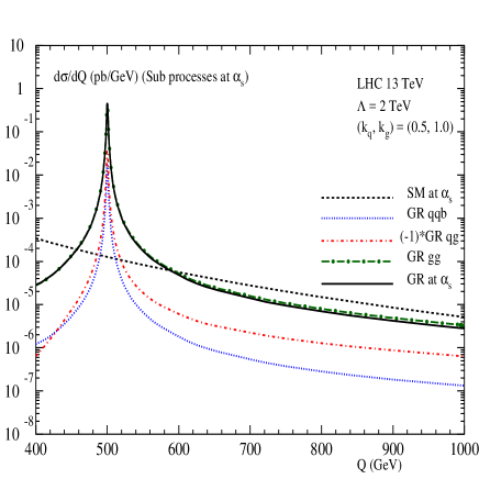
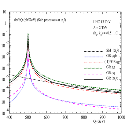
In our analysis, we restricted ourselves to the situation where spin-2 particle decays only to SM fields. The spin-2 particle decay widths for non-universal couplings are same as those given in Han:1998sg . For the scenario taken up here, where in all spin-2 coupling to all bosons are taken to be identical, we note that spin-2 particle decaying to $Z\gamma$ vanishes identically $\Gamma(h\to Z\gamma)=0$ Falkowski:2016glr . In fig.1, we present the NLO corrections (only at order $a_{s}$) from various subprocess contributions to the di-lepton production. For our default choice of model parameters, we find that $gg$ subprocess contribution dominates over the rest. In general, the total NLO correction is smaller than the $gg$ contribution because of negative contribution from $qg$ subprocess. We also note that the $gg$ has dominant contribution to the total decay width for couplings (0.5, 1.0).

To estimate the impact of QCD corrections, we define the K-factors as follows:

$$\text{K}_{1}=\frac{d\sigma^{\text{NLO}}/dQ}{d\sigma^{\text{LO}}/dQ}\qquad\text{and}\qquad\text{K}_{2}=\frac{d\sigma^{\text{NNLO}}/dQ}{d\sigma^{\text{LO}}/dQ}.$$ (23)

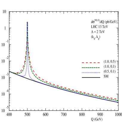
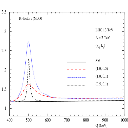
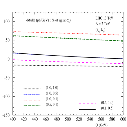
In the left panel of fig.2, we present di-lepton invariant mass distributions to NLO for different choices of non-universal couplings $(k_{q},k_{g})=(1.0,0.5),(1.0,0.1)$ and $(0.5,0.1)$. It is expected for universal couplings that at the resonance region, the cross sections i.e. the height of the peak will be the same simply because the couplings at the matrix element level will cancel with those from the decay width of the spin-2 particle. However, for non-universal couplings this is not the case and hence cross sections at the resonance for different non-universal couplings will be different. Thus, the precision as well as the phenomenological studies of the spin-2 particle production in this model will be different from those of the warped extra dimension models.The NLO K-factor ($K_{1}$) is present in the right panel for various choices of $(k_{q},k_{g})$ and we observe that the K-factor crucially depends on the choice of non-universal couplings. In particular we notice that the K-factors are larger for the choice of couplings (1.0,0.1). To understand this behaviour better, it is helpful to study the percentage contribution of various subprocesses to the total correction at NLO level, particularly from $qg$ subprocess due to its large flux at LHC energies. In particular we define the percentage of contribution of a given subprocess $ab$ as $R^{(i)}_{ab}=(d\sigma^{H_{1}H_{2},(i)}_{ab}/dQ^{2})/(d\sigma^{H_{1}H_{2},(i)}/dQ^{2})\times 100$, where the numerator is obtained by using contribution from $\Delta^{h,(i)}_{ab}$ and for the denominator, we include all the partonic channels.

In fig.3, we plot $R^{(1)}_{qg}$ for different choices of non-universal couplings and we observe that the sign of the $qg$ subprocess crucially depends on the choice of couplings. Moreover, we find that $R^{(1)}_{qg}$ is positive and is as large as $70\%$ for the couplings $(1.0,0.1)$, which explains the reason for the large K-factor at the resonance region. However, the sign of the contribution from other subprocesses $q\bar{q}$ and $gg$ is found to be positive for various couplings.

Figure 1: First order QCD corrections from different subprocesses to di-lepton production. The choice of the model parameters is as mentioned in the text.

Figure 2: Di-lepton invariant mass distributions are presented to NLO QCD for different choice of couplings ($k_{q},k_{g}$) in the left panel. The corresponding K-factors are presented in the right panel.

Figure 3: Percentage of $qg$ subprocess contribution $R^{(1)}_{qg}$ as defined in the text for different choice of non-universal couplings.

In fig.4, we present the second order QCD corrections (at $(a_{s}^{2})$) from various subprocesses to the di-lepton production for the default choice of couplings $(k_{q},k_{g})=(0.5,1.0)$. Similar to the first order QCD corrections, $gg$ subprocess has the dominant contribution over the rest while $qg$ has a negative contribution but is comparable in magnitude to that of $gg$. Because of this large $qg$ subprocess contribution which can flip its sign for certain couplings, it is necessary to study the percentage of its relative contribution $R^{(2)}_{qg}$ to the total second order correction.

Figure 4: Second order QCD corrections from various subprocess to the di-lepton invariant mass distribution.

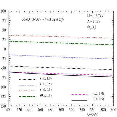
In fig.5, we present $R^{(2)}_{qg}$ for different choices of couplings. As can be seen from the figure, the $qg$ contribution varies from about $-70\%$ to about $35\%$ for the choice of couplings considered here. In particular, for the couplings $(1.0,0.1)$ and $(0.5,0.1)$ the $qg$ contribution is positive while it is negative for the rest of the couplings as well as in the SM. This implies large K-factors for the choice of $(1.0,0.1)$ couplings for a wide range of the invariant mass distribution. It is worth mentioning here that in general $qg$ subprocess has a negative contribution both in the SM as well as in the case of universal couplings, irrespective of the value of the latter.

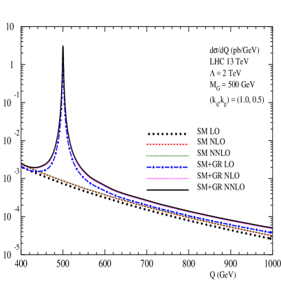
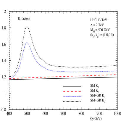
We then present the di-lepton invariant mass distribution to various orders in QCD for a particular choice of couplings $(1.0,0.5)$ in fig.6. In this case, the NLO QCD corrections for the signal (SM+spin-2) are as large as $60\%$ while those at NNLO, they are about $80\%$ at the resonance. Similar results are presented but for our default choice of model parameters in fig.7. Here, the corresponding NLO corrections to the signal are about $45\%$ while those of NNLO are about $55\%$.

Figure 5: Percentage of $qg$ contribution $R_{qg}^{(2)}$ as defined in the text.

Figure 6: cross sections at different orders (left panel) and the corresponding K-factors $K_{1}$ and $K_{2}$ (right panel) are presented for different couplings.

Figure 7: Same as fig.6 but for a different set of couplings.

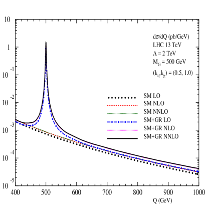
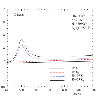
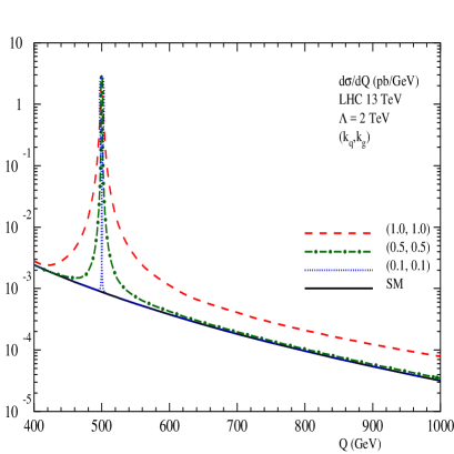
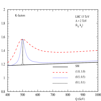
Next, we will study the invariant mass distributions of both the SM and the signal, in particular the impact of QCD corrections for different couplings. In fig.8,9,10, we present these distributions in the left panel and the corresponding NNLO K-factors $(K_{2})$ in the right panel for 9 different set of non-universal couplings. The respective K-factors for the signal at the resonance region are found to vary from about $1.5$ to about as large as $3.0$, owing to different contributions from $qg$ subprocess to the signal as explained before.

Figure 8: Di-lepton invariant mass distributions to NNLO for different choice of couplings (left panel) and the corresponding K-factors (right panel) are presented.

Figure 9: Same as fig.8 but for a different set of couplings.

Figure 10: Same as fig.8 but for a different set of couplings.

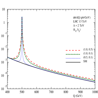
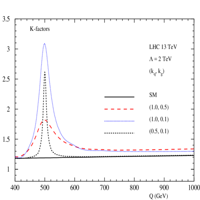
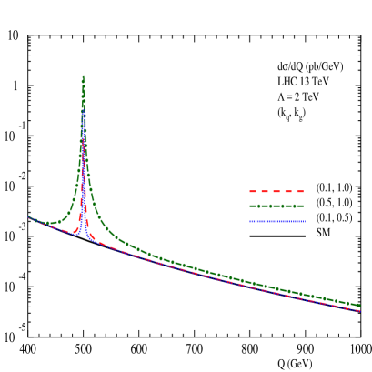
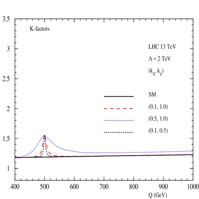
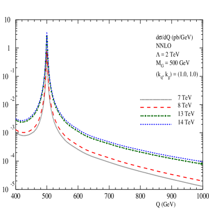
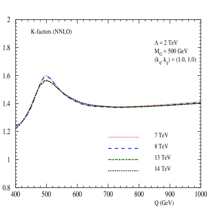
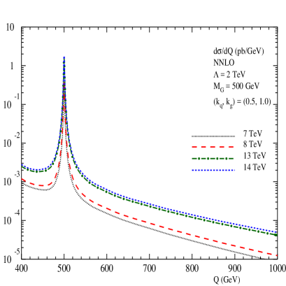
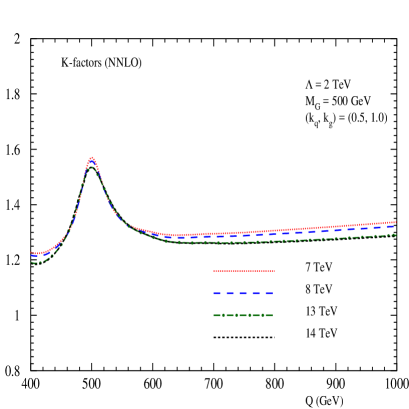
Further, we depict the dependence of invariant mass distributions to NNLO in QCD on the center of mass energy E${}_{\text{cm}}$ of the protons at the LHC. We present our results for E${}_{\text{cm}}=7,8,13$ and $14$ TeV energies for two different sets of couplings. In fig.11, we present the invariant mass distributions and the corresponding K-factors for the universal couplings of $(1.0,1.0)$. For default choice of non-universal couplings $(0.5,1.0)$, similar results are presented in fig.12. In both the cases, the K-factors at the resonance region are found to be larger for $7$ TeV case and are about $1.6$.

Figure 11: Dependence of cross sections on the di-lepton invariant mass distribution for universal couplings $(1.0,1.0)$.

Figure 12: Same as fig.11 but for the default choice of non-universal couplings $(0.5,1.0)$.

In what follows, we study the renormalization scale $\mu_{R}$ and the factorization scale $\mu_{F}$ uncertainties in our predictions. For this, we define the ratios $R(\mu_{R},\mu_{F})$ of the invariant mass distributions computed at arbitrary scale to those computed at the fixed scale. These are defined as

$$\text{R}(\mu_{R},\mu_{F})=\frac{d\sigma(\mu_{R},\mu_{F})/dQ}{d\sigma(Q_{0},Q_{0})/dQ}.$$

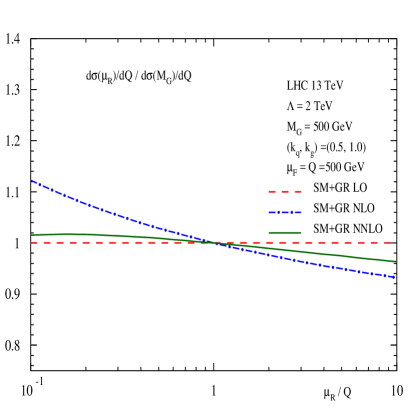
For a systematic study of these scale uncertainties, we use LO (NLO and NNLO) PDFs for LO (NLO and NNLO) cross sections respectively. For convenience, we will study at the resonance region i.e. $Q=M=500$ GeV. The fixed scale is set equal to $Q_{0}=M$. In the left panel of fig.13, we present $\text{R}(\mu_{R},Q_{0})$ by varying $\mu_{R}$ from $0.1Q$ to $10Q$ and keeping $\mu_{F}=Q_{0}$ fixed. At LO, there is no scale $\mu_{R}$ entering the cross section. The corresponding scale uncertainties at NLO and NNLO are respectively, about $19\%$ and $5\%$.

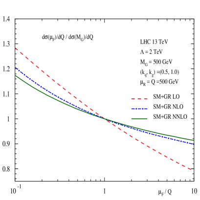
In the right panel of fig.13, we present $\text{R}(Q_{0},\mu_{F})$ by varying $\mu_{F}$ from $0.1Q$ to $10Q$ and keeping $\mu_{R}=Q_{0}$ fixed. For this range of factorization scale variation, the uncertainties in the distributions at LO, NLO and NNLO are respectively about $49\%$, $31\%$ and $26\%$.

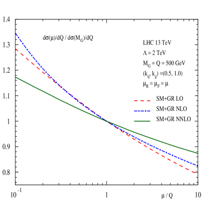
Finally, we present $\text{R}(\mu,\mu)$ (where $\mu_{R}=\mu_{F}=\mu$) in fig. 14 by varying $\mu$ from $0.1Q$ to $10Q$. The corresponding scale uncertainties at LO, NLO and NNLO are respectively about $49\%$, $52\%$ and $30\%$.

Figure 13: Renormalization (left) and factorization (right) scale dependence of the di-lepton invariant mass distribution at LO, NLO and NNLO.

Figure 14: Same as fig.13 but with $\mu_{R}=\mu_{F}=\mu$.

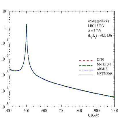
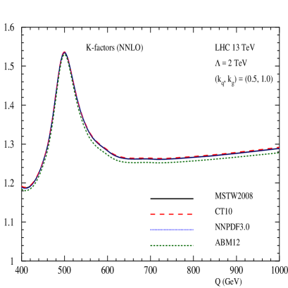
Before we summarize, we also study the uncertainties in our predictions due to different choice of PDFs used in the calculation. For this analysis, we make predictions using MSTW2008, CT10, NNPDF3.0 and ABM12 PDFs. The results for the invariant mass distributions for the signal at NNLO are presented in the left panel of fig.15 and the corresponding K-factors are presented in the right panel of fig.15. The K-factors here are found to vary from $1.18$ at $Q=400$ GeV to about $1.28$ at $Q=1000$ GeV, while at the resonance they are about $1.54$.

Figure 15: Di-lepton invariant mass distributions for different choice parton distribution functions (PDFs).

4 Conclusion

In this article, we have studied for the first time the impact of NNLO QCD corrections to the production of a pair of leptons in the presence of a massive spin-2 particle at the LHC. This is done in a minimal scenario where spin-2 particles couple differently to SM fermions and SM bosons. This task has been achieved by using the universal IR structure of QCD amplitudes and the additional UV renormalization that is particularly required for the case of non-universal couplings, thanks to the recent computations of the form factors in QCD beyond leading order with non-universal couplings.

Unlike the models with universal couplings, here the phenomenology is rich and different. For collider phenomenology at the LHC, we present the results for the di-lepton production via spin-2 particle in particular for the invariant mass distribution of a pair of leptons for LHC energies. Even at LO, one can notice that the signal has different cross sections at the resonance region in contrast to the gravity mediated models where the signal has the same cross section for different universal couplings. At higher orders in QCD, say NLO onwards, the spin-2 exploits its freedom of being produced with different coupling strengths even for a given subprocess. This particular aspect here makes the QCD radiative corrections crucially dependent on the choice of the spin-2 coupling strength. Hence the impact of QCD corrections here is very much different from those of di-lepton or Higgs production in the SM.

We find from our numerical results that the QCD corrections for $(k_{q},k_{g})=(1.0,0.1)$ are dominant over the rest of the choice of couplings, making the K-factors as large as 2.5 or more. For this choice of couplings, the LO gluon fusion contribution is very small although gluon fluxes are high for the kinematic region of producing a 500 GeV particle. But at higher orders where the spin-2 can be emitted off from a quark line with large coupling strength, the large quark-gluon fluxes at LHC energies can potentially enhance the spin-2 production rate, as is evident from the numerical results. For di-lepton production the ‘sign’ of $qg$ subprocess is usually negative both in the SM as well as in the models of universal couplings. But here we note that the ‘sign’ of $qg$ subprocess contribution changes with the non-universal couplings and for the above choice it is positive.

We also gave predictions for different center of mass energies of the incoming protons at the LHC and found that the K-factors are larger for 7 TeV case. We further quantified the renormalization and factorization scale uncertainties. For the variation of the scales $\mu_{R}$ and $\mu_{F}$ between $0.1Q$ and $10Q$, the uncertainties are found to get reduced from about 50% at LO to about 30% at NNLO. For completeness, we also quantified the uncertainty in our predictions due to different choice of the PDFs.

These NNLO QCD predictions for the hadroproduction of a massive spin-2 with non-universal couplings will augment the similar results previously computed at NLO level and compliment the earlier results for NNLO QCD corrections in models with spin-2/graviton universal couplings.

Appendix A Renormalized form factors

We present here the results for the renormalised form factors Ahmed:2016qjf that are used in the present computation. In the colour space, the UV renormalised matrix elements of composite operators ${\cal O}^{I},~{}I=G,Q$ between a pair of on-shell partonic states $i=q,g$ and the vacuum state are expanded in powers of coupling constant $a_{s}$ as

$$|\mathcal{M}^{I}_{i}\rangle=\sum_{n=0}^{\infty}{a}_{s}^{n}|\mathcal{M}^{I,(n)}_{i}\rangle$$ (24)

where $i=q,\overline{q},g$. The on-shell form factor of $\hat{\cal O}^{I},~{}I=G,Q$ are defined by taking the the overlap of $|\mathcal{M}^{I}_{i}\rangle$ with its leading order amplitude normalised with respect to the leading order contribution. We find that there are four independent form factors:

$${\cal F}^{I,g,(n)}=\frac{\langle{\mathcal{M}}^{G,(0)}_{g}|{\mathcal{M}}^{I,(n)}_{g}\rangle}{\langle{\mathcal{M}}^{G,(0)}_{g}|{\mathcal{M}}^{G,(0)}_{g}\rangle}\,,\hskip 28.45274pt{\cal F}^{I,q,(n)}=\frac{\langle{\mathcal{M}}^{Q,(0)}_{q}|{\mathcal{M}}^{I,(n)}_{q}\rangle}{\langle{\mathcal{M}}^{Q,(0)}_{q}|{\mathcal{M}}^{Q,(0)}_{q}\rangle}\quad\quad\quad I=G,Q\,.$$ (25)

Note that, the non-diagonal amplitudes i.e. $|{\mathcal{M}}^{Q,(n)}_{g}\rangle$ and $|{\mathcal{M}}^{G,(n)}_{q}\rangle$, start at one-loop level and hence, the corresponding form factors start at ${\cal O}({a}_{s})$. The relevant UV renormalised form factors up to two loop level are given below:

$$\mathcal{F}^{G,g,(1)} = {1\over\epsilon^{2}}C_{A}\Bigg{[}-8\Bigg{]}+{1\over\epsilon}\Bigg{[}C_{A}\Bigg{(}\frac{22}{3}\Bigg{)}+n_{f}\Bigg{(}-\frac{4}{3}\Bigg{)}\Bigg{]}+C_{A}\Bigg{[}-\frac{203}{18}+\zeta_{2}\Bigg{]}$$

$$+\epsilon C_{A}\Bigg{[}\frac{2879}{216}-\frac{7}{3}\zeta_{3}-\frac{11}{12}\zeta_{2}\Bigg{]}+\epsilon^{2}C_{A}\Bigg{[}-\frac{37307}{2592}+\frac{77}{36}\zeta_{3}+\frac{203}{144}\zeta_{2}+\frac{47}{80}\zeta_{2}^{2}\Bigg{]}\,,$$

$$\mathcal{F}^{G,g,(2)} = {1\over\epsilon^{4}}C_{A}^{2}\Bigg{[}32\Bigg{]}+{1\over\epsilon^{3}}\Bigg{[}C_{A}^{2}\Bigg{(}-\frac{308}{3}\Bigg{)}+n_{f}C_{A}\Bigg{(}\frac{56}{3}\Bigg{)}\Bigg{]}+{1\over\epsilon^{2}}\Bigg{[}C_{A}^{2}\Bigg{(}\frac{1162}{9}-4\zeta_{2}\Bigg{)}$$

$$+n_{f}C_{A}\Bigg{(}-\frac{52}{3}\Bigg{)}+n_{f}^{2}\Bigg{(}\frac{16}{9}\Bigg{)}\Bigg{]}+{1\over\epsilon}\Bigg{[}C_{A}^{2}\Bigg{(}-\frac{4420}{27}+\frac{50}{3}\zeta_{3}+11\zeta_{2}\Bigg{)}$$

$$+n_{f}C_{A}\Bigg{(}\frac{278}{27}-\frac{2}{3}\zeta_{2}\Bigg{)}+n_{f}C_{F}\Bigg{(}-2\Bigg{)}\Bigg{]}+C_{A}^{2}\Bigg{(}\frac{11854}{81}-\frac{253}{9}\zeta_{3}-\frac{94}{9}\zeta_{2}$$

$$-\frac{21}{5}\zeta_{2}^{2}\Bigg{)}+n_{f}C_{A}\Bigg{(}\frac{1105}{162}+2\zeta_{3}-\frac{26}{9}\zeta_{2}\Bigg{)}+n_{f}C_{F}\Bigg{(}\frac{1049}{162}-\frac{16}{9}\zeta_{2}\Bigg{)}\,,$$

$$\mathcal{F}^{G,q,(1)} = C_{F}\Bigg{(}\frac{34}{9}\Bigg{)}+\epsilon C_{F}\Bigg{(}-\frac{79}{27}+\frac{2}{3}\zeta_{2}\Bigg{)}+\epsilon^{2}C_{F}\Bigg{(}\frac{401}{162}-\frac{14}{9}\zeta_{3}-\frac{17}{36}\zeta_{2}\Bigg{)}\,,$$

$$\mathcal{F}^{G,q,(2)} = {1\over\epsilon^{2}}C_{F}^{2}\Bigg{(}-\frac{272}{9}\Bigg{)}+{1\over\epsilon}C_{F}^{2}\Bigg{(}\frac{1244}{27}-\frac{16}{3}\zeta_{2}\Bigg{)}+C_{F}C_{A}\Bigg{(}\frac{3913}{81}+\frac{28}{9}\zeta_{2}\Bigg{)}$$

$$+C_{F}^{2}\Bigg{(}-\frac{2603}{27}+\frac{112}{9}\zeta_{3}+\frac{56}{3}\zeta_{2}\Bigg{)}+n_{f}C_{F}\Bigg{(}-\frac{1166}{81}\Bigg{)}\,,$$

$$\mathcal{F}^{Q,g,(1)} = n_{f}\Bigg{(}\frac{35}{18}\Bigg{)}+\epsilon n_{f}\Bigg{(}-\frac{497}{216}+\frac{1}{6}\zeta_{2}\Bigg{)}+\epsilon^{2}n_{f}\Bigg{(}\frac{6593}{2592}-\frac{7}{18}\zeta_{3}-\frac{35}{144}\zeta_{2}\Bigg{)}\,,$$

$$\mathcal{F}^{Q,g,(2)} = {1\over\epsilon^{2}}n_{f}C_{A}\Bigg{(}-\frac{140}{9}\Bigg{)}+{1\over\epsilon}\Bigg{[}n_{f}C_{A}\Bigg{(}\frac{98}{3}-\frac{4}{3}\zeta_{2}\Bigg{)}+n_{f}^{2}\Bigg{(}-\frac{70}{27}\Bigg{)}\Bigg{]}$$

$$+n_{f}C_{A}\Bigg{(}-\frac{7625}{162}+\frac{100}{9}\zeta_{3}+\frac{53}{9}\zeta_{2}\Bigg{)}+n_{f}C_{F}\Bigg{(}\frac{299}{81}-8\zeta_{3}+\frac{16}{9}\zeta_{2}\Bigg{)}$$

$$+n_{f}^{2}\Bigg{(}\frac{497}{162}-\frac{2}{9}\zeta_{2}\Bigg{)}\,,$$

$$\mathcal{F}^{Q,q,(1)} = {1\over\epsilon^{2}}C_{F}\Bigg{(}-8\Bigg{)}+{1\over\epsilon}C_{F}\Bigg{(}6\Bigg{)}+C_{F}\Bigg{(}-\frac{124}{9}+\zeta_{2}\Bigg{)}$$

$$+\epsilon C_{F}\Bigg{(}\frac{403}{27}-\frac{7}{3}\zeta_{3}-\frac{17}{12}\zeta_{2}\Bigg{)}+\epsilon^{2}C_{F}\Bigg{(}-\frac{2507}{162}+\frac{119}{36}\zeta_{3}+\frac{31}{18}\zeta_{2}+\frac{47}{80}\zeta_{2}^{2}\Bigg{)}\,,$$

$$\mathcal{F}^{Q,q,(2)} = {1\over\epsilon^{4}}C_{F}^{2}\Bigg{(}32\Bigg{)}+{1\over\epsilon^{3}}\Bigg{[}C_{F}C_{A}\Bigg{(}-44\Bigg{)}+C_{F}^{2}\Bigg{(}-48\Bigg{)}$$ (26)

$$+n_{f}C_{F}\Bigg{(}8\Bigg{)}\Bigg{]}+{1\over\epsilon^{2}}\Bigg{[}C_{F}C_{A}\Bigg{(}\frac{64}{9}+4\zeta_{2}\Bigg{)}+C_{F}^{2}\Bigg{(}\frac{1154}{9}-8\zeta_{2}\Bigg{)}$$

$$+n_{f}C_{F}\Bigg{(}-\frac{16}{9}\Bigg{)}\Bigg{]}+{1\over\epsilon}\Bigg{[}C_{F}C_{A}\Bigg{(}\frac{961}{54}-26\zeta_{3}+11\zeta_{2}\Bigg{)}+C_{F}^{2}\Bigg{(}-\frac{10831}{54}$$

$$+\frac{128}{3}\zeta_{3}+\frac{16}{3}\zeta_{2}\Bigg{)}+n_{f}C_{F}\Bigg{(}-\frac{65}{27}-2\zeta_{2}\Bigg{)}\Bigg{]}+C_{F}C_{A}\Bigg{(}-\frac{31495}{216}+\frac{601}{9}\zeta_{3}$$

$$-\frac{73}{2}\zeta_{2}+\frac{44}{5}\zeta_{2}^{2}\Bigg{)}+C_{F}^{2}\Bigg{(}\frac{68677}{216}-\frac{922}{9}\zeta_{3}+\frac{11}{6}\zeta_{2}-13\zeta_{2}^{2}\Bigg{)}$$

$$+n_{f}C_{F}\Bigg{(}\frac{9469}{324}+\frac{2}{9}\zeta_{3}+\frac{47}{9}\zeta_{2}\Bigg{)}\Bigg{]}\,.$$

References

- (1) ATLAS collaboration, G. Aad et al., Observation of a new particle in the search for the Standard Model Higgs boson with the ATLAS detector at the LHC, Phys. Lett. B716 (2012) 1–29, [1207.7214].
- (2) CMS collaboration, S. Chatrchyan et al., Observation of a new boson at a mass of 125 GeV with the CMS experiment at the LHC, Phys. Lett. B716 (2012) 30–61, [1207.7235].
- (3) R. V. Harlander and W. B. Kilgore, Next-to-next-to-leading order Higgs production at hadron colliders, Phys. Rev. Lett. 88 (2002) 201801, [hep-ph/0201206].
- (4) C. Anastasiou and K. Melnikov, Higgs boson production at hadron colliders in NNLO QCD, Nucl. Phys. B646 (2002) 220–256, [hep-ph/0207004].
- (5) V. Ravindran, J. Smith and W. L. van Neerven, NNLO corrections to the total cross-section for Higgs boson production in hadron hadron collisions, Nucl. Phys. B665 (2003) 325–366.
- (6) G. Degrassi, S. Di Vita, J. Elias-Miro, J. R. Espinosa, G. F. Giudice, G. Isidori et al., Higgs mass and vacuum stability in the Standard Model at NNLO, JHEP 08 (2012) 098, [1205.6497].
- (7) L. Randall and R. Sundrum, A Large mass hierarchy from a small extra dimension, Phys. Rev. Lett. 83 (1999) 3370–3373, [hep-ph/9905221].
- (8) CMS collaboration, V. Khachatryan et al., Search for high-mass diphoton resonances in proton–proton collisions at 13 TeV and combination with 8 TeV search, Phys. Lett. B767 (2017) 147–170, [1609.02507].
- (9) ATLAS collaboration, M. Aaboud et al., Search for diboson resonances with boson-tagged jets in collisions at TeV with the ATLAS detector, Phys. Lett. B777 (2018) 91–113, [1708.04445].
- (10) P. Artoisenet et al., A framework for Higgs characterisation, JHEP 11 (2013) 043, [1306.6464].
- (11) T. Ahmed, P. Banerjee, P. K. Dhani, P. Mathews, N. Rana and V. Ravindran, Three loop form factors of a massive spin-2 particle with nonuniversal coupling, Phys. Rev. D95 (2017) 034035, [1612.00024].
- (12) N. K. Nielsen, The Energy Momentum Tensor in a Nonabelian Quark Gluon Theory, Nucl. Phys. B120 (1977) 212–220.
- (13) P. Mathews, V. Ravindran, K. Sridhar and W. L. van Neerven, Next-to-leading order QCD corrections to the Drell-Yan cross section in models of TeV-scale gravity, Nucl. Phys. B713 (2005) 333–377, [hep-ph/0411018].
- (14) P. Mathews and V. Ravindran, Angular distribution of Drell-Yan process at hadron colliders to NLO-QCD in models of TeV scale gravity, Nucl. Phys. B753 (2006) 1–15, [hep-ph/0507250].
- (15) M. C. Kumar, P. Mathews and V. Ravindran, PDF and scale uncertainties of various DY distributions in ADD and RS models at hadron colliders, Eur. Phys. J. C49 (2007) 599–611, [hep-ph/0604135].
- (16) M. C. Kumar, P. Mathews, V. Ravindran and A. Tripathi, Diphoton signals in theories with large extra dimensions to NLO QCD at hadron colliders, Phys. Lett. B672 (2009) 45–50, [0811.1670].
- (17) M. C. Kumar, P. Mathews, V. Ravindran and A. Tripathi, Direct photon pair production at the LHC to order in TeV scale gravity models, Nucl. Phys. B818 (2009) 28–51, [0902.4894].
- (18) N. Agarwal, V. Ravindran, V. K. Tiwari and A. Tripathi, Z boson pair production at the LHC to O(alpha(s)) in TeV scale gravity models, Nucl. Phys. B830 (2010) 248–270, [0909.2651].
- (19) N. Agarwal, V. Ravindran, V. K. Tiwari and A. Tripathi, Next-to-leading order QCD corrections to the boson pair production at the LHC in Randall Sundrum model, Phys. Lett. B686 (2010) 244–248, [0910.1551].
- (20) N. Agarwal, V. Ravindran, V. K. Tiwari and A. Tripathi, production in Large extra dimension model at next-to-leading order in QCD at the LHC, Phys. Rev. D82 (2010) 036001, [1003.5450].
- (21) N. Agarwal, V. Ravindran, V. K. Tiwari and A. Tripathi, Next-to-leading order QCD corrections to production at the LHC in Randall Sundrum model, Phys. Lett. B690 (2010) 390–395, [1003.5445].
- (22) R. Frederix, M. K. Mandal, P. Mathews, V. Ravindran, S. Seth, P. Torrielli et al., Diphoton production in the ADD model to NLO+parton shower accuracy at the LHC, JHEP 12 (2012) 102, [1209.6527].
- (23) R. Frederix, M. K. Mandal, P. Mathews, V. Ravindran and S. Seth, Drell-Yan, production in SM & ADD model to NLO+PS accuracy at the LHC, Eur. Phys. J. C74 (2014) 2745, [1307.7013].
- (24) G. Das, P. Mathews, V. Ravindran and S. Seth, RS resonance in di-final state production at the LHC to NLO+PS accuracy, JHEP 10 (2014) 188, [1408.3970].
- (25) G. Das, C. Degrande, V. Hirschi, F. Maltoni and H.-S. Shao, NLO predictions for the production of a (750 GeV) spin-two particle at the LHC, 1605.09359.
- (26) D. de Florian, M. Mahakhud, P. Mathews, J. Mazzitelli and V. Ravindran, Quark and gluon spin-2 form factors to two-loops in QCD, JHEP 02 (2014) 035, [1312.6528].
- (27) D. de Florian, M. Mahakhud, P. Mathews, J. Mazzitelli and V. Ravindran, Next-to-Next-to-Leading Order QCD Corrections in Models of TeV-Scale Gravity, JHEP 04 (2014) 028, [1312.7173].
- (28) T. Ahmed, P. Banerjee, P. K. Dhani, M. C. Kumar, P. Mathews, N. Rana et al., NNLO QCD Corrections to the Drell-Yan Cross Section in Models of TeV-Scale Gravity, 1606.08454.
- (29) T. Ahmed, M. Mahakhud, P. Mathews, N. Rana and V. Ravindran, Two-Loop QCD Correction to massive spin-2 resonance 3 gluons, JHEP 05 (2014) 107, [1404.0028].
- (30) T. Ahmed, G. Das, P. Mathews, N. Rana and V. Ravindran, The two-loop QCD correction to massive spin-2 resonance , Eur. Phys. J. C76 (2016) 667, [1608.05906].
- (31) ATLAS collaboration, G. Aad et al., Study of the spin and parity of the Higgs boson in diboson decays with the ATLAS detector, Eur. Phys. J. C75 (2015) 476, [1506.05669].
- (32) L. E. Pedersen, Probing the nature of the Higgs Boson: A study of the Higgs spin and parity through the final state at the ATLAS Experiment. PhD thesis, Bohr Inst., 2015.
- (33) T. Han, J. D. Lykken and R.-J. Zhang, On Kaluza-Klein states from large extra dimensions, Phys. Rev. D59 (1999) 105006, [hep-ph/9811350].
- (34) P. Mathews, V. Ravindran and K. Sridhar, NLO - QCD corrections to e+ e- —¿ hadrons in models of TeV-scale gravity, JHEP 08 (2004) 048, [hep-ph/0405292].
- (35) G. Altarelli, R. K. Ellis and G. Martinelli, Leptoproduction and Drell-Yan Processes Beyond the Leading Approximation in Chromodynamics, Nucl. Phys. B143 (1978) 521.
- (36) T. Matsuura and W. L. van Neerven, Second Order Logarithmic Corrections to the Drell-Yan Cross-section, Z. Phys. C38 (1988) 623.
- (37) T. Matsuura, S. C. van der Marck and W. L. van Neerven, The Calculation of the Second Order Soft and Virtual Contributions to the Drell-Yan Cross-Section, Nucl. Phys. B319 (1989) 570–622.
- (38) R. Hamberg, W. L. van Neerven and T. Matsuura, A complete calculation of the order correction to the Drell-Yan factor, Nucl. Phys. B359 (1991) 343–405.
- (39) T. Ahmed, M. Mahakhud, N. Rana and V. Ravindran, Drell-Yan Production at Threshold to Third Order in QCD, Phys. Rev. Lett. 113 (2014) 112002, [1404.0366].
- (40) F. V. Tkachov, A Theorem on Analytical Calculability of Four Loop Renormalization Group Functions, Phys. Lett. B100 (1981) 65–68.
- (41) K. Chetyrkin and F. Tkachov, Integration by Parts: The Algorithm to Calculate beta Functions in 4 Loops, Nucl.Phys. B192 (1981) 159–204.
- (42) T. Gehrmann and E. Remiddi, Differential equations for two loop four point functions, Nucl.Phys. B580 (2000) 485–518.
- (43) C. Anastasiou, C. Duhr, F. Dulat, E. Furlan, T. Gehrmann, F. Herzog et al., Higgs boson gluon–fusion production at threshold in N3LO QCD, Phys. Lett. B737 (2014) 325–328, [1403.4616].
- (44) C. Anastasiou, C. Duhr, F. Dulat, F. Herzog and B. Mistlberger, Higgs Boson Gluon-Fusion Production in QCD at Three Loops, Phys. Rev. Lett. 114 (2015) 212001, [1503.06056].
- (45) C. Anastasiou, C. Duhr, F. Dulat, E. Furlan, T. Gehrmann, F. Herzog et al., High precision determination of the gluon fusion Higgs boson cross-section at the LHC, JHEP 05 (2016) 058, [1602.00695].
- (46) T. Kinoshita, Mass singularities of Feynman amplitudes, J. Math. Phys. 3 (1962) 650–677.
- (47) T. D. Lee and M. Nauenberg, Degenerate Systems and Mass Singularities, Phys. Rev. 133 (1964) B1549–B1562.
- (48) D. J. Gross and F. Wilczek, Ultraviolet Behavior of Nonabelian Gauge Theories, Phys. Rev. Lett. 30 (1973) 1343–1346.
- (49) H. D. Politzer, Reliable Perturbative Results for Strong Interactions?, Phys. Rev. Lett. 30 (1973) 1346–1349.
- (50) W. E. Caswell, Asymptotic Behavior of Nonabelian Gauge Theories to Two Loop Order, Phys. Rev. Lett. 33 (1974) 244.
- (51) O. V. Tarasov and A. A. Vladimirov, Three Loop Calculations in Non-Abelian Gauge Theories, Phys. Part. Nucl. 44 (2013) 791–802, [1301.5645].
- (52) S. A. Larin and J. A. M. Vermaseren, The Three loop QCD Beta function and anomalous dimensions, Phys. Lett. B303 (1993) 334–336, [hep-ph/9302208].
- (53) G. Altarelli and G. Parisi, Asymptotic Freedom in Parton Language, Nucl. Phys. B126 (1977) 298–318.
- (54) E. G. Floratos, R. Lacaze and C. Kounnas, Space and Timelike Cut Vertices in QCD Beyond the Leading Order. 2. The Singlet Sector, Phys. Lett. 98B (1981) 285–290.
- (55) E. G. Floratos, R. Lacaze and C. Kounnas, Space and Timelike Cut Vertices in QCD Beyond the Leading Order. 1. Nonsinglet Sector, Phys. Lett. 98B (1981) 89–95.
- (56) G. Curci, W. Furmanski and R. Petronzio, Evolution of Parton Densities Beyond Leading Order: The Nonsinglet Case, Nucl. Phys. B175 (1980) 27–92.
- (57) S. Moch, J. A. M. Vermaseren and A. Vogt, The Three loop splitting functions in QCD: The Nonsinglet case, Nucl. Phys. B688 (2004) 101–134, [hep-ph/0403192].
- (58) A. Vogt, S. Moch and J. A. M. Vermaseren, The Three-loop splitting functions in QCD: The Singlet case, Nucl. Phys. B691 (2004) 129–181, [hep-ph/0404111].
- (59) A. Falkowski and J. F. Kamenik, Diphoton portal to warped gravity, Phys. Rev. D94 (2016) 015008, [1603.06980].