Perturbed Kitaev model: excitation spectrum and long-ranged spin correlations.

Abstract

We developed general approach to the calculation of power-law infrared asymptotics of spin-spin correlation functions in the Kitaev honeycomb model with different types of perturbations. We have shown that in order to find these correlation functions, one can perform averaging of some bilinear forms composed out of free Majorana fermions, and we presented the method for explicit calculation of these fermionic densities. We demonstrated how to derive an effective Hamiltonian for the Majorana fermions, including the effects of perturbations. For specific application of the general theory, we have studied the effect of the Dzyaloshinskii-Moriya anisotropic spin-spin interaction; we demonstrated that it leads, already in the second order over its relative magnitude $D/K$, to a power-law spin correlation functions, and calculated dynamical spin structure factor of the system. We have shown that an external magnetic field $h$ in presence of the DM interaction, opens a gap in the excitation spectrum of magnitude $\Delta\propto Dh$.

I Introduction

Quantum spin liquids (QSL) (see e.g. Refs. Anderson, 1973; Fazekas and Anderson, 1974; Wen, 2002; Lhuillier and Misguich, 2001; Misguich, 2008; Balents, 2010; Savary and Balents, 2016) present examples of strongly correlated quantum phases not developing any kind of local order in spite of vanishing specific entropy at zero temperature. Critical, or algebraic QSL’s are characterized by spin correlation functions decaying with distance (time) as certain powers. An exactly solvable case of the critical QSL is provided by the celebrated Kitaev honeycomb spin model Kitaev (2006) (see also Ref. Nussinov and Brink, 2013). This model was originally invented as a simplest solvable spin model possessing nontrivial topological phases, relevant in the context of topological quantum computing; later it has been found that similar spin interactions can be realized in the honeycomb-lattice oxidesJackeli and Khaliullin (2009) Na₂IrO₃ and Li₂IrO₃. Kitaev honeycomb model Hamiltonian reads

$$\mathcal{H_{K}}=K\sum_{\left\langle ij\right\rangle\in\alpha\beta(\gamma)}\sigma_{i}^{\alpha}\sigma_{j}^{\alpha}$$ (1)

where each of $\sigma_{i}^{\alpha}$ represents a Pauli matrices corresponding to $i$-th site of the honeycomb lattice. There are 3 types of bonds (see Fig. 1) which are denoted below as $xy(z)$,$yz(x)$ and $zx(y)$. Although long-range spin correlations vanish exactly in the model Eq (1), its spectrum contains gapless fermions and hence it presents a convenient starting point for the construction of controllable theories possessing long-range spin correlations. In a realistic situation, low-energy effective description of these materials is given by a mixture of the Kitaev and Heisenberg (and other) interactions with weights depending on the microscopic parametersChaloupka et al. (2013); Winter et al. (2016) (for recent reviews on ”Kitaev materials” see Refs. Trebst, 2017; Winter et al., 2017.). Another interesting appearance of Heisenberg-Kitaev (HK) model is in a low-energy theory of a Hubbard model on a honeycomb lattice with spin-dependent hoppingHassan et al. (2013). An important question is to which extent the properties of the ground state (and excitations) of the perturbed Kitaev model are proximate to that of the unperturbed one? Exact diagonalization and a complementary spin-wave analysisChaloupka et al. (2010) show that spin-liquid phase near the Kitaev limit is stable with respect to small admixture of Heisenberg interactionsReuther et al. (2011); Schaffer et al. (2012). From experimental side, although there was no report of detection of a spin-liquid state realized by this scenario in the absence of external magnetic field, the importance of the Kitaev interaction has been clearly demonstrated in $\alpha$-RuCl₃Banerjee et al. (2016, 2017); Plumb et al. (2014); Sandilands et al. (2015); Kim et al. (2015); Janša et al. (2017) and Na₂IrO₃ Chun et al. (2015); Choi et al. (2012); Alpichshev et al. (2015). Moreover, in two recent Refs. Baek et al., 2017 and Hentrich et al., 2017 the data are present in favor of a spin liquid state in $\alpha$-RuCl₃ realized upon application of external magnetic field.

As we have already mentioned, Kitaev model in its original form does not possess long-range spin correlations; moreover, its spin correlators are strictly localBaskaran et al. (2007). A perturbative addition of the Heisenberg interaction does not change this factMandal et al. (2011a). In order to produce a spin-liquid phase with long-range correlations, some other terms should be added to the effective Hamiltonian. The simplest perturbation which does not destroy spin-liquid phase but renders correlations non-local is magnetic fieldTikhonov et al. (2011) (the HK model with magnetic field was also studied in Refs Trousselet et al., 2011; Jiang et al., 2011). A more general picture of emergence of spin correlations in the Kitaev model due to various perturbation was discussed recently in Ref. Song et al., 2016. In the present paper, we develop a general scheme in which the long-distance (time) spin-spin correlation functions in Kitaev honeycomb model with various types of local perturbations can be analysed. In quite a general form, we have reduced the calculation of spin-spin correlation functions to evaluation of specific correlation functions bilinear forms of free Majorana fermion. We have also studied effects of higher-order terms and found the effective Hamiltonian for Majorana fermions modified by weak perturbations of the spin Hamiltonian. Besides explaining qualitative differences between results previously obtained for various perturbationsTikhonov et al. (2011); Song et al. (2016), we considered the effect of Dzyaloshinksi-Moria (DM) interaction and demonstrated that it leads to the power-law correlations already in the lowest possible (second) order over its strength $D/K$. We have also found that application of magnetic field $\mathbf{h}$ to a model, perturbed by DM interaction, produces the gap $\Delta\sim Dh/K$ in the Majorana fermion spectrum, rendering decay of spin correlations in space and time exponential. Note in this respect that linear growth of the spin-liquid excitation gap has been recently observedBaek et al. (2017); Hentrich et al. (2017) in $\alpha$-RuCl₃.

II Kitaev honeycomb model with perturbations: a brief review

The model (1) was solved Kitaev (2006) via an exact transformation to Majorana fermion representation (similar procedure using the language of Jordan-Wigner transformation was later developed in Ref. Chen and Nussinov, 2008), which is constructed as follows. For each lattice site $i$ one defines 4 Majorana fermions $b^{x}_{i}$, $b^{y}_{i}$, $b^{z}_{i}$ and $c_{i}$. Our goal is to reproduce the algebra of Pauli matrices using these fermions, which is achieved by the substitution $\sigma_{i}^{\alpha}=ib^{\alpha}_{i}c_{i}$. However, the number of degrees of freedom is larger in the Majorana representation (4 states per site) than in the spin-$\frac{1}{2}$ representation: each pair of Majorana fermions is equivalent to one usual complex fermion, so to each site two fermions are attached, which is equivalent to 2 spin-$\frac{1}{2}$ variables. This problem is fixed by the constraint imposed on the Majorana operators while acting in the ”physical subspace”  of the full Hilbert space of the Majorana operators: $b^{x}_{i}b^{y}_{i}b^{z}_{i}c_{i}=1$. This condition is due to the identity $\sigma^{x}\sigma^{y}\sigma^{z}=i$ valid for Pauli matrices.

After the substitution of the spin operators in terms of Majorana variables, the Hamiltonian becomes

$$H=-iK\sum_{\langle i,j\rangle\in\alpha\beta(\gamma)}b_{i}^{\gamma}b_{j}^{\gamma}c_{i}c_{j}$$ (2)

The honeycomb lattice contains two sublattices and each edge connects vertices from different sublattices. Let us take as convention that for each bond of the lattice in the above sum $i\in$ the first sublattice and $j\in$ the second one. Then for each of the bonds $\langle i,j\rangle\in\alpha\beta(\gamma)$ there exists a conserved quantity $u_{ij}=ib^{\gamma}_{i}b^{\gamma}_{j}$: such an operator commutes with the Hamiltonian. The operator $u_{ij}$ also anti-commutes with $\sigma^{\gamma}_{i}$ or $\sigma^{\gamma}_{j}$, and also $u_{ij}^{2}=1$, thus $u_{ij}=\pm 1$ for all eigenstates. As we have already mentioned above, the Majorana representation has extra degrees of freedom w.r.t. the original Pauli matrix representation. These extra degrees of freedom are partially accounted for by the constraints $b^{x}_{i}b^{y}_{i}b^{z}_{i}c_{i}=1$. Another extra degree of freedom is related to the gauge transformation: for any particular site $i$ we can replace $b^{\alpha}_{i}\rightarrow-b^{\alpha}_{i}$ and $c_{i}\rightarrow-c_{i}$; in result, all $u_{ij}$, where $j$ is a neighbour of $i$, change its sign. Gauge independent integrals of motion, called ”fluxes”, are defined for all plaquettes of the lattice, see Fig. 1. For each plaquette $p$ a flux operator is defined as $w_{p}=\prod_{\langle i,j\rangle\in p}u_{ij}$ (1). Evidently, $w_{p}^{2}=1$, thus $w_{p}=\pm 1$ for all eigenstates. If some $w_{p}=-1$, we say that there is a flux associated with the $p$-th plaquette. It can be shownLieb (2004) that the ground state contains no fluxes. Thus, up to possible gauge transformations, in the ground state all $u_{ij}=1$. As a result, the Majorana Hamiltonian can be written in the following form:

$$H=-iK\sum_{\langle ij\rangle}c_{i}c_{j}$$ (3)

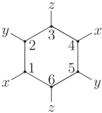
Figure 1: Definition of gauge-invariant integrals of motion $W_{p}=u_{21}u_{61}u_{65}u_{45}u_{43}u_{23}=\sigma^{x}_{1}\sigma^{y}_{2}\sigma^{z}_{3}\sigma^{x}_{4}\sigma^{y}_{5}\sigma^{z}_{6}$.

Fourier transformation of the Hamiltonian (3) leads to the free-particle spectrum $\varepsilon(\mathbf{p})=|f(\mathbf{p})|$ where

$$f(\mathbf{p})=2K(e^{i(\mathbf{n}_{1},\mathbf{p})}+e^{i(\mathbf{n}_{2},\mathbf{p})}+1)$$

and $\mathbf{n}_{1}=\left(\begin{smallmatrix}\frac{1}{2}\\ \frac{\sqrt{3}}{2}\end{smallmatrix}\right)$ and $\mathbf{n}_{2}=\left(\begin{smallmatrix}-\frac{1}{2}\\ \frac{\sqrt{3}}{2}\end{smallmatrix}\right)$ are the translation vectors of the lattice (lattice constant is set to unity). Here $x$ axis is perpendicular the $z$-bonds, while $y$ axis is parallel the $z$-bonds (see Fig. 1). This energy spectrum possesses two conical points: $\mathbf{Q}_{1,2}=\left(\begin{smallmatrix}\pm\frac{2\pi}{3}\\ \frac{2\pi}{\sqrt{3}}\end{smallmatrix}\right)$. Near these points $\varepsilon(\mathbf{p})$ vanishes linearly with $|\mathbf{p}-\mathbf{Q}_{1,2}|$.

For a system with a spectrum containing conical points, one would expect a power-law decay of correlation functions at long times and large space separations. However, it is not true for the Kitaev model as was highlighted in Ref. Baskaran et al., 2007 demonstrated that spin correlations vanish for any distance $i-j$ longer than just single bond length. Such a strange behavior originates from exact integrability of the model. Indeed, any spin operator $\sigma^{\alpha}_{i}$ anticommutes with all bond variables $u_{ij}$; as a result, the action of a spin operator on the flux-less ground state is to create two fluxes located in the plaquettes $p_{1,2}^{i,j}$ adjacent to the bond $(ij)$. In order for the correlation function $\langle T\sigma_{i}^{\alpha}(t)\sigma_{j}^{\beta}(0)\rangle$ to be nonzero, fluxes created by the spin operator $\sigma_{i}^{\alpha}$ must be annihilated by another operator $\sigma_{j}^{\beta}$, since overlap between quantum states with different flux content is zero due to conservation of the fluxes (integrability). The above condition for flux cancellation cannot be fulfilled for $|i-j|>1$, leading to vanishing of such spin correlations. It is evident from the above discussion that small perturbations, which weakly destroy integrability of the Kitaev model, allow for the ”revival”   of spin correlations at large distances. The type of these correlations (exponential vs power-law decay Mandal et al. (2011a); Tikhonov et al. (2011)) depends upon the flux content of the perturbing operator, as we discuss below.

Let us first describe the relevant perturbations to the Kitaev Hamiltonian. As magnetic materials with heavy elements contain strong spin-orbit interactions responsible for establishing the interaction of the form of Eq. (1), it is necessary to classify the states in terms of total angular momentum $K$, without separation into spin and orbital parts. In a number of cases low-energy excitations of such a system can be described in terms of effective variables, formally equivalent to spin-$\frac{1}{2}$. In some magnetic materials (for example, $Na_{2}IrO_{3}$, $\alpha$-RuCl₃, $\alpha$-Li₂IrO₃, see Ref. Winter et al., 2016) the anisotropic Kitaev term is the largest in magnitude. However, the full Hamiltonian contains also other terms which can possibly be treated as perturbations to the Kitaev Hamiltonian. Most typical perturbations are known to be isotropic Heisenberg interaction and pseudodipolar interaction:

$$V_{H}=\sum_{\langle i,j\rangle}J(\vec{\sigma_{i}},\vec{\sigma_{j}})\quad\mbox{Heisenberg interaction }$$ (4)

$$V_{\Gamma}=\sum_{\langle i,j\rangle\in\alpha\beta(\gamma)}\Gamma^{\gamma}_{ij}(\sigma^{\alpha}_{i}\sigma^{\beta}_{j}+\sigma^{\alpha}_{j}\sigma^{\beta}_{i})\quad\mbox{ pseudodipolar interaction}$$ (5)

Many different ground-states can be realized Rau et al. (2014) depending upon specific relations between energy parameters $K$, $J$ and $\Gamma$: ferromagnetic, anti-ferromagnetic, zigzag or stripy types of ordered states, as well as spin-liquid state in some narrow range of the full parameter space.

More detailed microscopic study of effective spin interactions, conducted in Ref. Winter et al., 2016 demonstrated relevance of DM interactions. In particular it is interesting to consider the effect of the DM anisotropic interaction. It was found that DM interaction between nearest neighbours is absent in this system due to inversion symmetry of the microscopic Hamiltonian. Interaction between next-nearest-neighbours

$$V_{DM}=\sum_{\langle\langle i,j\rangle\rangle}(\vec{D}_{ij},[\vec{\sigma}_{i},\vec{\sigma}_{j}]).$$ (6)

is compatible with inversion symmetry. The honeycomb lattice possesses three different types of next-nearest-neighbours. Each of them can be put into one-to-one correspondence with nearest-neighbours directions $\alpha$: if the pair of next-nearest-neighbours is connected by a segment which is perpendicular to the $\alpha$ direction, we will denote this segment as $\alpha_{2}$, and the corresponding vector characterizing DM interaction will be denoted as $\vec{D}_{\alpha_{2}}$. In our further analysis, only single component of each such DM vector is involved, namely for $\alpha=x,y,z$ we write $D^{\alpha}$ for $\alpha$-s component of $\vec{D}_{\alpha_{2}}$ and introduce $D=\sqrt{(D^{x})^{2}+(D^{y})^{2}+(D^{z})^{2}}$.

Typical values of various interaction constants for several ”Kitaev materials” were computed in Winter et al. (2016), they are presented in the table below (in units of meV).

	$K$	$J$	$\Gamma$	$D$
Na2IrO3	$-16.2$	$1.6$	$2.1$	$0.17$
$\alpha$-RuCl3	$-7.5$	$-2.2$	$8.0$	$0.44$
$\alpha$-Li2IrO3	$-13.0$	$-4.6$	$11.6$	$0.44$

For the general analysis of the role of perturbations, the Hamiltonian of system can be presented in the form

$$H=H_{K}+\sum_{n}V_{n},$$ (7)

where $n$ enumerates different types of local perturbations. The spin-spin correlation function is then given by the perturbation theory expansion

$$S^{\alpha\beta}_{ij}(t)=\langle T\sigma^{\alpha}_{i}(t)\sigma_{j}^{\beta}(0)\rangle=\sum_{n}\frac{(-i)^{n}}{n!}\sum_{k_{1}\ldots k_{n}}\int d\tau_{1}\ldots d\tau_{n}\langle T\sigma^{\alpha}_{i}(t)\sigma_{j}^{\beta}(0)V_{k_{1}}(\tau_{1})\ldots V_{k_{n}}(\tau_{n})\rangle.$$ (8)

The ground state average in Eq. (8) vanishes if the product of operators $\sigma^{\alpha}_{i}\sigma_{j}^{\beta}V_{k_{1}}\ldots V_{k_{n}}$ creates fluxes. To get a nonzero result, the product of perturbation operators $V_{k_{1}}\ldots V_{k_{n}}$ should create the same fluxes as the product of spin operators $\sigma^{\alpha}_{i}\sigma_{j}^{\beta}$ does. Two qualitatively different situations may occur, leading to either power-law, or exponential decay of spin correlations with a distance $|i-j|$.

Power-law decay is realized if the product of some number of perturbation operators $V_{k}$ can be represented in the form $V_{k_{1}}\ldots V_{k_{n}}=V_{i,\alpha}V_{j,\beta}$, where $V_{i,\alpha}$ creates the same fluxes as the spin operator $\sigma_{i}^{\alpha}$, and $V_{j,\beta}$ creates the same fluxes as the spin operator $\sigma_{j}^{\beta}$. Then the necessary number $n$ of the operators $V_{k}$ in the product $V_{k_{1}}\ldots V_{k_{n}}$ does not grow with the distance $|i-j|$. Such a situation is realized by the magnetic field perturbation Tikhonov et al. (2011) with

$$V_{h}^{z}=-h^{z}\sum_{i}\sigma_{i}^{z},$$ (9)

with flux pattern illustrated on the Fig. 2a as well as by the combined Heisenberg and pseudodipolar interactions Song et al. (2016) where $V=V_{H}+V_{\Gamma}$. The first mentioned case is the simplest one: long-range spin-spin correlation $S^{zz}_{ij}(t)$ contains an overall coefficient $h_{z}^{2}$, as follows from the above analysis in terms of flux creation/annihilation. The second case Song et al. (2016) appears to be more delicate. Namely, a straightforward counting of fluxes indicates appearance of long-range correlations with a coefficient $\propto(\Gamma J)^{2}$. Indeed, such terms appear in the perturbation theory, but they cancel completely due to some special symmetry reasons, and nonzero contribution was found in the next order of perturbation theory, so it scales as $S^{\alpha\beta}_{ij}(t)\propto(\Gamma J)^{4}$. This observation demonstrates that analysis of fluxes is not sufficient, in general, to determine the lowest necessary order of the perturbation that leads to long-range correlations. More detailed analysis of the relevant symmetries will be presented below in the end of the Sec. V.

Exponential decay of correlation functions with distance takes place if perturbation terms are not able to annihilate ”locally”   the fluxes created by spin operators $\sigma_{i}^{\alpha}$ and $\sigma_{j}^{\beta}$. In such case the necessary result - complete flux annihilation - can be achieved in the $n$-th order of perturbation theory only, where $n\sim|i-j|$, thus in this case correlation functions decrease exponentially with a distance Mandal et al. (2011b). However, the above arguments do not imply exponential decay of correlation functions with time $t$, thus in this situation unusual asymmetry of space-time correlations may be expected; this issue needs further studies. An example of exponential spatial decay of correlations is provided by purely Heisenberg perturbation $\hat{V}_{H}$. Each of such terms create fluxes in 4 plaquettes, as shown in Fig.2b. Consecutive action of operators $\hat{V}_{H}$ ordered along the line between sites $i$ and $j$ consists in the moving pairs of fluxes from the vicinity of the site $i$ where these fluxes were created, to the vicinity of the site $j$ where they will be annihilated. Thus the minimal number of such operators is $\sim n$ and the whole correlation function is bounded from above by $(J/K)^{n}\sim\exp\left(-n\ln\frac{K}{J}\right)$.

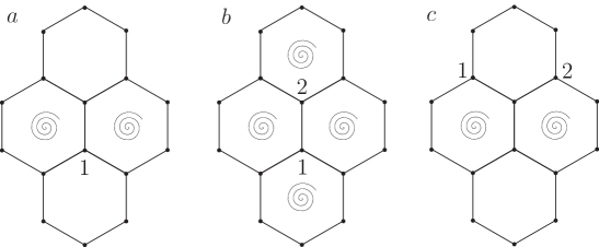
Figure 2: Flux patterns created by various perturbations. (2a) Magnetic field: $\sigma_{1}^{z}$, (2b) Heisenberg interaction: one specific term $\sigma_{1}^{x}\sigma_{2}^{x}$, (2c) DM interaction: one specific term $\sigma_{1}^{y}\sigma_{2}^{x}$.

III Reduction of spin correlation function to fermionic representation.

Below we consider the Hamiltonians of the form

$$\mathcal{H}=\mathcal{H_{K}}+\sum_{i\in even,\alpha}V_{i}^{\alpha}.$$ (10)

Here by $V_{i}^{\alpha}$ we denote an operator which is  i) composed out of spin operators, and   ii) creates the same combination of fluxes as the operator $\sigma_{i}^{\alpha}$, or, equivalently, $\sigma^{\alpha}_{i+\alpha}$. The site notation $i+\alpha$ means that this site is connected to the site $i$ by a bond of the $\alpha$ type. Summation over $i\in even$ in the second term of (10) means that these $i$ sites belong to the even sublattice of the honeycomb lattice; below we identify $V^{\alpha}_{i+\alpha}=V_{i}^{\alpha}$. Particular examples of the models (10) are provided by the Kitaev model with a magnetic (9) field and/or with the second-neighbours DM interaction (6).

We are interested in the calculation of the correlation function of spin operators $S^{\alpha\beta}_{ij}(t)=\langle T\sigma_{i}^{\alpha}(t)\sigma^{\beta}_{j}(0)\rangle$, for large distances $r=|i-j|\gg 1$ between sites $i$ and $j$, and at long time intervals $Kt\gg 1$. Below we will show that such a correlation function can be represented in terms of correlations of fermionic bilinear operators:

$$S^{\alpha\beta}_{i,j}(t)=\langle T\sigma_{i}^{\alpha}(t)\sigma_{j}^{\beta}(0)\rangle=\langle TQ_{i}^{\alpha}(t)Q_{j}^{\beta}(0)\rangle,$$ (11)

where

$$Q_{i}^{\alpha}=\frac{i}{2}\sum_{c_{a},c_{b}\in\{c^{(i)}_{1}\ldots c^{(i)}_{n}\}}V^{\alpha}_{i,ab}c_{a}c_{b},$$ (12)

and matrix elements:

$$V^{\alpha}_{i,ab}=\int^{\infty}_{0}d\tau\langle V_{i}^{\alpha}(\tau)\sigma_{i}^{\alpha}(0)c_{a}(0)c_{b}(0)\rangle+\int^{0}_{-\infty}\langle c_{a}(0)c_{b}(0)\sigma(0)_{i}^{\alpha}V_{i}^{\alpha}(\tau)\rangle d\tau$$ (13)

In the above equation, the variables $c^{(i)}_{a}$ denote fermionic operators located near $c_{i}$ and defined in terms of the fermionic content of the operator product $\sigma_{i}^{\alpha}V_{i}^{\alpha}$:

$$\sigma_{i}^{\alpha}V_{i}^{\alpha}=A_{i}c^{(i)}_{1}\ldots c^{(i)}_{n_{i}}U_{i}$$ (14)

where $U_{i}$ is some product of the bond integrals of motions ($u_{pq}$), while $A_{i}$ is some constant.

Matrix elements $V^{\alpha}_{i,ab}$ can also be written in terms of spin correlation functions. The simplest example is provided by $V_{i}^{\alpha}=\sigma_{i+\alpha}$. In this case $Q^{\alpha}_{i}=i\gamma_{i}h^{\alpha}V_{h}c_{i}c_{i+\alpha}$, where $\gamma_{i}=1$ if $i$ belongs to the even sublattice and $\gamma_{i}=-1$ otherwise. For the matrix element $V_{h}$ one finds then $V_{h}=2\int_{0}^{\infty}\langle\sigma_{i}^{z}(\tau)\sigma_{i}^{z}(0)\rangle d\tau$.

Now we proceed with the derivation of the representation (11), (12) and (13) for spin correlation function. If $V_{i}^{\alpha}$ is a product of spin operators, the first non-zero term of the perturbation expansion (8) is of the second order in $V_{i}^{\alpha}$:

$$S^{\alpha\beta}_{ij}(t)=\langle T\sigma^{\alpha}_{i}(t)\sigma^{\beta}_{j}(0)\rangle=-\int d\tau_{1}d\tau_{2}\langle T\sigma^{\alpha}_{i}(t)\sigma^{\beta}_{j}(0)V^{\alpha}_{i}(\tau_{1})V^{\beta}_{j}(\tau_{2})\rangle.$$ (15)

The main contribution to the integrals in Eq.(15) comes from the region where $|t-\tau_{1}|K\sim 1$ and $|\tau_{2}|K\sim 1$, see Ref. Tikhonov et al., 2011. There are 4 possible variants of the time ordering in this region. Let us consider just one of them as an example:

$$S^{(I)}=-\int^{t}_{0}d\tau_{1}\int^{\tau_{1}}_{0}d\tau_{2}\langle\sigma^{\alpha}_{i}(t)V^{\alpha}_{i}(\tau_{1})V^{\beta}_{j}(\tau_{2})\sigma^{\beta}_{j}(0)\rangle.$$ (16)

To shorten further notations, we define operators $\tilde{V}_{i}^{\alpha}$ via the following identity:

$$V_{i}^{\alpha}\tilde{V}_{i}^{\alpha}=[H,V_{i}^{\alpha}].$$ (17)

Operators with tilde sign do not create fluxes, they are of the second order in Majorana variables, and each of the fermionic bilinear contains fermions which belong to different sublattices. With the definition (17), we represent correlation function (16) in the form

$$S^{(I)}=-\int^{t}_{0}d\tau_{1}\int^{\tau_{1}}_{0}d\tau_{2}\langle e^{iHt}\sigma^{\alpha}_{i}V^{\alpha}_{i}e^{-i(H+\tilde{V}_{i}^{\alpha})(t-\tau_{1})}e^{-iH(\tau_{1}-\tau_{2})}e^{-i(H+\tilde{V}^{\beta}_{j})\tau_{2}}V^{\beta}_{j}\sigma^{\beta}_{j}\rangle,$$ (18)

which can be further transformed using representation of operators entering Eq.(18) in terms of $c_{a}$ and $u_{ab}$ via Eq.(14). The result of this transformation reads:

$$S^{(I)}=-\int^{t}_{0}d\tau_{1}\int^{\tau_{1}}_{0}d\tau_{2}\langle TA_{i}c^{(i)}_{1}(t)\ldots c^{(i)}_{n_{i}}(t)A_{j}c^{(j)}_{1}(0)\ldots c^{(j)}_{n_{j}}(0)e^{-i(\int_{\tau_{1}}^{t}\tilde{V}_{i}^{\alpha}(\tau^{\prime})d\tau^{\prime}+\int^{\tau_{2}}_{0}\tilde{V}_{j}^{\beta}(\tau^{\prime})d\tau^{\prime})}\rangle.$$ (19)

The above correlation function describes non-interacting Majorana fermions living in the time-dependent potential, which is switched on/off for some intervals of time. Thus we come to a kind of problem similar to the celebrated Fermi-edge singularities Nozieres and De Dominicis (1969). The key difference consists in the zero density of states at the Fermi level in our problem (due to conical spectrum and fixed at $\epsilon=0$ position of the Fermi-level). This is the reason for the absence of the ”orthogonality catastrophe”    Anderson (1967) in our case.

We analyse now the average of a product of Majorana operators, Eq. (19), by means of diagram technique in terms of free Majorana Green functions $G_{ab}(t)=\langle Tc_{a}(t)c_{b}(0)\rangle$, using Wick theorem. The key observation is based upon the fact that we are studing infrared asymptotics, $(r,Kt)\gg 1$, and the corresponding Green functions decay rather quickly with distance and time, $G_{ij}\propto(\max(r,Kt)^{-2})$, where $r$ is distance between $i$ and $j$. For this reason, any irreducible diagram, entering the average in (19), should contain exactly two ”nonlocal”   Green functions (nonlocal is an average of 2 fermion operators such that one of them is located near $c_{i}$ and the other near $c_{j}$). Apart from these two nonlocal lines, an arbitrary number of local Majorana Green functions (containing both fermionic operators located near point $i$ or near point $j$) may enter various diagrams originating from Eq.(19). One of typical diagrams of such a type is shown in Fig. 3 for the specific case of the DM perturbation.

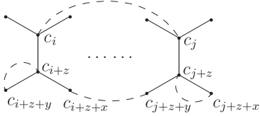
Figure 3: One of the diagram for evaluation of the spin correlation function in the presence DM interaction: dashed lines are for Majorana Green function. Two of the pairings involve fermions, separated by large distance with the rest paired in the vicinity of each of the spin operators (applied at points $i$ and $j$).

Summation of all these diagrams can be represented analytically in the following form:

$$S^{(I)}=-\frac{1}{4}\sum_{a,b,p,q}\langle Tc_{a}(t)c_{b}(t)c_{p}(0)c_{q}(0)\rangle\int^{t}_{0}d\tau_{1}\int^{\tau_{1}}_{0}d\tau_{2}\langle c_{a}(t)c_{b}(t)\sigma(t)_{i}^{\alpha}V_{i}^{\alpha}(\tau_{1})\rangle\langle V_{j}^{\beta}(\tau_{2})\sigma_{j}^{\beta}(0)c_{p}(0)c_{q}(0)\rangle.$$ (20)

In the expression above, the first average of four Majorana operators contains two non-local Green functions. Second and third averages contains two sets of local diagrams, located near the points $i$ and $j$ respectively. Identity $c_{a}^{2}=1$ was used to represent the diagrams in the form (20). The main contribution to the integral over $d\tau_{1}$ and $d\tau_{2}$ in Eq.(20) comes from the region where $K|t-\tau_{1}|\sim 1$ and $K\tau_{2}\sim 1$; taking into account the condition $K|t|\gg 1$, we can extend the limits of integration over $d\tau_{1,2}$ to infinity. Finally, taking into account all possible versions of time ordering, we obtain representaion (11-13) for spin correlation function.

The above analysis can be generalized to the case when perturbation $V$ contain several operators $V_{1}$, $\ldots$, $V_{n}$, and their product creates the same pattern of fluxes as $\sigma_{i}^{\alpha}$ does, as well as for the operator $\sigma_{j}^{\beta}$. We still can write spin-spin correlation function in the form of Eq. ( 11), while expressions (12,13) should be modified. Namely, Majorana operators $c_{a}$ and $c_{b}$ which enter $Q_{i}^{\alpha}$ are those operators, which are contained in the operator product $\sigma_{i}^{\alpha}V_{1}\ldots V_{n}$ when it is expressed in terms of Maiorana variables $c_{i}$ and bond variables $u_{ij}$. Generalized expression for matrix elements $V_{ab}$ now reads as follows:

$$V_{ab}=\sum_{k=0}^{n}\sum_{\zeta=\langle i_{1}\ldots i_{n}\rangle\in S_{n}}\xi_{ab,\zeta,k}\int_{0}^{\infty}d\tau_{1}\int_{0}^{\tau_{1}}d\tau_{2}\ldots\int_{0}^{\tau_{k-1}}d\tau_{k}\int_{-\infty}^{0}d\tau_{k+1}\ldots\int_{-\infty}^{\tau_{n-1}}d\tau_{n}$$

$$\langle V_{i_{1}}(\tau_{1})\ldots V_{i_{k}}(\tau_{k})c_{a}(0)c_{b}(0)\sigma_{i}^{\alpha}(0)V_{i_{k+1}}(\tau_{k+1})\ldots V_{i_{n}}(\tau_{n})\rangle.$$ (21)

Here $\zeta$ is some permutation of numbers $1,\ldots n$, and $\xi_{ab,\zeta,k}=\pm 1$ are defined via an identity $c_{a}c_{b}V_{i_{1}}\ldots V_{i_{k}}=\xi_{ab,\zeta,k}V_{i_{1}}\ldots V_{i_{k}}c_{a}c_{b}$. In the term with $k=0$ all $\tau_{i}<0$, while the term with $k=n$ contains all $\tau_{i}>0$.

Let us now see how this general treatment applies to some particular example. We will consider Kitaev model, perturbed by small magnetic field, studied in Ref. Tikhonov et al., 2011. This is described by Eq. (10) with $V_{i}^{\alpha}=-h^{\alpha}(\sigma_{i}^{\alpha}+\sigma_{i+\alpha}^{\alpha})$, giving

$$Q^{\alpha}_{i}=i\gamma_{i}h^{\alpha}V_{h}c_{i}c_{i+\alpha},$$ (22)

with $\gamma_{i}=\pm 1$ for lattice site $i$ in the even/odd sublattice correspondingly and numerical coefficient $V_{h}=2\int_{0}^{\infty}\langle\sigma_{i}^{z}(\tau)\sigma_{i}^{z}(0)\rangle d\tau$. Substituting Eq. (22) to Eq. (11), we obtain at large $\max(r,t)$ (but far from the mass shell $|r-\sqrt{3}Kt|\gg 1$):

$$S^{\alpha\beta}(\mathbf{r},t)_{ij}=\frac{h^{\alpha}h^{\beta}V_{h}^{2}}{\pi^{2}(r^{2}-3K^{2}t^{2})^{3}}\{r^{2}\sin\left[\frac{2\pi}{3}(\mathbf{e}_{x},\mathbf{n}_{\beta}+\mathbf{r})-\phi_{x}\right]\sin\left[\frac{2\pi}{3}(\mathbf{e}_{x},\mathbf{n}_{\alpha}-\mathbf{r})-\phi_{x}\right]$$

$$-3K^{2}t^{2}\cos\left[\frac{2\pi}{3}(\mathbf{e}_{x},(\mathbf{n}_{\alpha}-\mathbf{n}_{\beta}-\mathbf{r}))\right]\cos\left[\frac{2\pi}{3}(\mathbf{r},\mathbf{e}_{x})\right]\}.$$ (23)

In this equation, we have assumed for simplicity that $i$ and $j$ belong to the even sublattice and introduced $\mathbf{n}_{x}=2\mathbf{n}_{1}$, $\mathbf{n}_{y}=2\mathbf{n}_{2}$, $\mathbf{n}_{z}=\mathbf{0}$, $\mathbf{e}_{x}$ for the unit vector along $x$ axis and $\phi_{x}$ for the angle between $\mathbf{r}$ and $\mathbf{e}_{x}$. In the case of either $i$ or $j$ belonging to the odd sublattice, one can use identity $Q_{i+\alpha}^{\alpha}=Q_{i}^{\alpha}$ in order to generalize Eq.(23).

The structure factor which is Fourier transform of correlation function in this case demonstrates interesting behaviour near three points in the Brillouin zone, located at $(0,0)$, $\mathbf{q}_{+}=2\mathbf{e_{x}}$ and $\mathbf{q}_{-}=-\mathbf{q}_{+}$. Near $(0,0)$ it is given by

$$S^{\alpha\beta}(\mathbf{q},\omega)-S(\mathbf{0},0)=\frac{h^{\alpha}h^{\beta}V_{h}^{2}\theta(\omega^{2}-3K^{2}q^{2})}{8\sqrt{\omega^{2}-3K^{2}q^{2}}}\{q^{2}+(2\omega^{2}-3K^{2}q^{2})\cos(\frac{2\pi}{3}(\mathbf{e}_{x},\mathbf{n}_{\alpha}-\mathbf{n}_{\beta}))\},$$ (24)

while near $\mathbf{q}_{\pm}$ the structure factor varies as

$$S^{\alpha\beta}(\mathbf{q},\omega)-S(\mathbf{q}_{\pm},0)=\frac{h^{\alpha}h^{\beta}V_{h}^{2}\theta(\omega^{2}-3K^{2}q^{2})}{4}\sqrt{\omega^{2}-3K^{2}q^{2}}e^{\mp i\frac{2\pi}{3}(\mathbf{e}_{x},\mathbf{n}_{\alpha}-\mathbf{n}_{\beta})}.$$ (25)

IV Effective Majorana Hamiltonian

As we have discussed above, one of the effects of the perturbations on the Kitaev model is to couple the spin density to local bilinear Fermionic operators. However, it is natural to expect that a general perturbation is also able to modify the dynamics of Fermionic operators themselves. Indeed, as was demonstrated by Kitaev Kitaev (2006), magnetic field $h$ treated perturbatively in the 3rd order opens a gap in the fermionic spectrum, proportional to $h_{x}h_{y}h_{z}$. We will now analyse the effects of high-order terms in the perturbation theory for a more generic perturbation. Consider the following Hamiltonian:

$$H=H_{K}+\sum_{n}\left[V_{n,1}+V_{n,2}\right].$$ (26)

In this equation, we have explicitly introduced two contributions to the perturbing Hamiltonian, $V_{n,1}$ and $V_{n,2}$ which create the same flux pattern when applied to the ground state of unperturbed model. We will assume that $V_{n,\xi}$ are products of spin operators. Our goal will be to study the perturbation theory series for the Fermionic Green function and resum it in the low-energy limit. Let us first present our result. We have found that corrections to the Green function in this limit are described by the following correction to the Fermionic Hamiltonian:

$$\delta H=\frac{(-i)}{4}\sum_{m}\sum_{p,q}c_{p}c_{q}V_{m,pq},$$ (27)

with numerical coefficients given by:

$$V_{m,pq}=\int_{0}^{\infty}d\tau\langle V_{m,1}(\tau)V_{m,2}(0)c_{p}(0)c_{q}(0)\rangle+\int_{-\infty}^{0}\langle c_{p}(0)c_{q}(0)V_{m,2}(0)V_{m,1}(\tau)\rangle d\tau+(1\leftrightarrow 2).$$ (28)

Majorana fermions $c_{p}$ and $c_{q}$ entering Eq.(28) are contained in the operator product $V_{m,1}V_{m,2}$, in the same sense as it was indicated in Eq. (14) regarding operator product $\sigma_{i}^{\alpha}V_{i}^{\alpha}$.

Let us explain how this result can be derived. We start from perturbation theory series for the Green function:

$$G_{ij}(t)=\sum_{n}\frac{(-i)^{n}}{n!}\sum_{m_{i},\xi_{i},\zeta_{i}}\int d\tau_{1}\ldots d\tau_{n}\langle Tc_{i}(t)c_{j}(0)V_{m_{1},\xi_{1}}(\tau_{1})\ldots V_{m_{n},\xi_{n}}(\tau_{n})\rangle$$ (29)

The average of an operator in Eq. (29) is non-zero only when it is flux-free, which requires $n$ to be even and all $V_{m,\xi}$ to be separable into flux-free pairs. As operators in each pair appear at different instants of time, the flux does exist for short (of the order of $K^{-1}$) periods of time. As $tK\gg 1$, time intervals between pairs are larger than $K^{-1}$. Thus, we can rewrite (29):

$$G_{ij}(t)=\sum_{n}\frac{(-i)^{2n}}{n!2^{n}}\sum_{m_{i},\xi_{i},\zeta_{i}}\int d\tau_{1}\ldots d\tau_{2m}\langle Tc_{i}(t)c_{j}(0)V_{m_{1},\xi_{1}}(\tau_{1})V_{m_{1},\zeta_{1}}(\tau_{2})\ldots V_{m_{n},\xi_{n}}(\tau_{2n-1})V_{m_{n},\zeta_{n}}(\tau_{2n})\rangle$$

(30)

For each $n$ there are $2^{n}$ different contributions ($\tau_{2l-1}>\tau_{2l}$ or $\tau_{2l}>\tau_{2l-1}$ for all $l=1\ldots n$). Let us consider one of them:

$$\delta G_{ij}(t)=\sum_{n}\frac{(-i)^{2n}}{2^{n}}\sum_{m_{i},\xi_{i},\zeta_{i}}\int_{-\infty}^{\infty}d\tau_{1}\int_{-\infty}^{\tau_{1}}d\tau_{2}\ldots\int_{-\infty}^{\tau_{2m}-1}d\tau_{2m}$$

$$\langle Tc_{i}(t)c_{j}(0)V_{m_{1},\xi_{1}}(\tau_{1})V_{m_{1},\zeta_{1}}(\tau_{2})\ldots V_{m_{n},\xi_{n}}(\tau_{2n-1})V_{m_{n},\zeta_{n}}(\tau_{2n})\rangle.$$

(31)

Using commutation relations (17), we can now bring together operators in each flux-free pair together (similarly to the calculation of the spin-spin correlation function):

$$\delta G_{ij}(t)=\sum_{n}\frac{(-i)^{2n}}{2^{n}}\sum_{m_{i},\xi_{i},\zeta_{i}}\int_{-\infty}^{\infty}d\tau_{1}\int_{-\infty}^{\tau_{1}}d\tau_{2}\ldots\int_{-\infty}^{\tau_{2m}-1}d\tau_{2m}$$

$$\langle Tc_{i}(t)c_{j}(0)V_{m_{1},\xi_{1}}(\tau_{1})V_{m_{1},\zeta_{1}}(\tau_{1})\ldots V_{m_{n},\xi_{n}}(\tau_{2n-1})V_{m_{n},\zeta_{n}}(\tau_{2n-1})e^{-i\int\tilde{V}(\tau^{\prime})d\tau^{\prime}}\rangle,$$

(32)

where $\tilde{V}$ stays for the scattering potential induced by the fluxes. Similarly to Eq. (19), to obtain the main contribution we need only an open line contributions containing non-local Green functions, joining distant points, with all other Green functions being are ’local’. Upon this selection, we obtain the following expression:

$$\delta G_{ij}(t)=\sum_{n}\frac{(-i)^{2n}}{2^{2n}}\sum_{m_{1},\xi_{1},\zeta_{1}\ldots m_{n},\xi_{n},\zeta_{n}}\sum_{p_{1},q_{1},\ldots p_{n},q_{n}}\int_{-\infty}^{\infty}d\tau_{1}\int_{-\infty}^{\tau_{1}}d\tau_{2}\ldots\int_{-\infty}^{\tau_{2m}-1}d\tau_{2m}$$

$$\langle Tc_{i}(t)c_{j}(0)c_{p_{1}}(\tau_{1})c_{p_{2}}(\tau_{1})\ldots c_{p_{n}}(\tau_{n})c_{q_{n}}(\tau_{n})\rangle$$

$$\langle c_{p_{1}}(\tau_{1})c_{q_{1}}(\tau_{1})V_{m_{1},\xi_{1}}(\tau_{1})V_{m_{1},\zeta_{1}}(\tau_{2})\rangle\ldots\rangle c_{p_{n}}(\tau_{2n-1})c_{q_{n}}(\tau_{2n-1})V_{m_{n},\xi_{n}}(\tau_{2n-1})V_{m_{n},\zeta_{n}}(\tau_{2n})\rangle.$$

(33)

As in Eq. (20), the first average in Eq. (33) describes non-local diagram pairings and the remaining $n$ averages describe local Green function near $m_{1}$,$\ldots$,$m_{n}$ respectively. Indices $p_{i}$ and $q_{i}$ enumerate all Majoranas which appear in the expression for $V_{m_{i},1}V_{m_{i},2}$ expanded using Eq. (14). After summation of all $2^{n}$ contributions (a number of different time orderings), we find that correction to the Green function is reproduced by effective Hamiltonian in Eq. (27).

As a similar result for the correlation function, see Eq. (21), this result for effective Hamiltonian can be generalized. In a more general situation, one may have not a pair of perturbing terms $V_{1},\;V_{2}$, which is flux-free but a larger combination, say, $V_{1},\;\ldots,\;V_{n}$. In this case, correction to the low-energy Hamiltonian becomes as follows:

$$\delta H=\frac{-i}{4}\sum_{a,b}V_{ab}c_{a}c_{b},$$ (34)

where $c_{a}$ and $c_{b}$ are fermions, which enter the product $V_{1}\ldots V_{n}$, expanded in terms of Majoranas $c_{i}$ and conserved quantities $u_{ij}$. The matrix elements in this effective Hamiltonian read:

$$V_{ab}=\sum_{k=1}^{n}\sum_{\zeta=\langle i_{1}\ldots i_{n}\rangle\in S_{n}}\xi_{ab,\zeta,k}\int_{0}^{\infty}d\tau_{1}\int_{0}^{\tau_{1}}d\tau_{2}\ldots\int_{0}^{\tau_{k-1}}d\tau_{k}\int_{-\infty}^{0}d\tau_{k+2}\ldots\int_{-\infty}^{\tau_{n-1}}d\tau_{n}$$

$$\langle V_{i_{1}}(\tau_{1})\ldots V_{i_{k}}(\tau_{k})c_{a}(0)c_{b}(0)V_{i_{k+1}}(0)V_{i_{k+2}}(\tau_{k+2})\ldots V_{i_{n}}(\tau_{n})\rangle.$$ (35)

In this equation, $\zeta$ is a permutation of $1,\ldots n$ and $\xi_{ab,\zeta,k}=\pm 1$ is introduced according to the following identity:

$$c_{a}c_{b}V_{i_{1}}\ldots V_{i_{k}}=\xi_{ab,\zeta,k}V_{i_{1}}\ldots V_{i_{k}}c_{a}c_{b}.$$ (36)

The boundary cases of $\tau_{i}$ in Eq. (35) should be understood as follows: for $k=0$ all $\tau_{i}<0$ and for $k=n$ all $\tau_{i}>0$.

V Implications of time-reversal symmetry

In general, evaluation of matrix elements $V_{ab}$ in (13) and (27) is a complicated task. However, some of their properties follow directly from the properties of the spin perturbation with respect to time inversion. Expressions for matrix elements have similar form:

$$V=\int_{0}^{\infty}\langle V_{1}(\tau)V_{2}(0)\rangle d\tau-\int_{-\infty}^{0}\langle V_{2}^{\dagger}(0)V^{\dagger}_{1}(\tau)\rangle d\tau,$$ (37)

where $V_{1}=V_{i}^{\alpha}$ and $V_{2}=\sigma_{i}^{\alpha}c_{a}c_{b}$ (note that $V_{1,2}$ are not necessarily Hermitian). These operators can be written in terms of spins operators with the same flux patterns. The coefficients $V_{a,b}$ in Eqs. (12), (27) have the same structure. It is convenient to represent operators $V_{1,2}$ as $V_{\alpha}=\eta_{\alpha}C_{\alpha}B_{\alpha}$ with $\alpha=1,2$, $\eta$ for some constant, $C$ for a product of $c_{i}$ and $B$ for a product of $b_{i}$. Using commutation relations (17) we can write Eq. (37) (up to the sign of the whole expression) as follows:

$$\pm V=\eta_{1}\eta_{2}\int_{0}^{\infty}\langle TC_{1}(\tau)C_{2}(0)B_{1}(0)B_{2}(0)e^{-i\int_{0}^{\tau}\tilde{B}_{1}(\tau^{\prime})d\tau^{\prime}}\rangle-\eta_{1}^{*}\eta_{2}^{*}\int_{-\infty}^{0}\langle TB_{2}^{\dagger}(0)B_{1}^{\dagger}(0)C_{2}^{\dagger}(0)C_{1}^{\dagger}(\tau)e^{-i\int_{\tau}^{0}\tilde{B}_{1}(\tau^{\prime})d\tau^{\prime}}\rangle d\tau.$$

(38)

The operator $\tilde{B}_{1}$ is defined similarly to the operator $\tilde{V}$, see Eq. (17). The operator $B_{1}B_{2}$ contains only $b_{i}$, it is flux-free and equals to some constant $b$ under the average. In what follows, we will consider both averages in Eq. (38) expanding it via Wick theorem. As $c_{i}=c_{i}^{\dagger}$, all operators in different terms in (38) are the same but are ordered differently. Importantly, $G_{11}$ and $G_{22}$ are odd functions of time and $G_{12}$ and $G_{21}$ are even. To rearrange $C_{2}^{\dagger}C_{1}^{\dagger}$ into $C_{1}C_{2}$ under the sign of T-average we need $\frac{N(N-1)}{2}$ transpositions, where $N$ is the total number of fermionic operators in $C_{1}C_{2}$. We can change a sign of integration time variables in the second term and use properties of time reversal symmetry of Green functions. After such a change, it will have acquire a sign $(-1)^{m}$ where $m$ is a number of Green functions $G_{11}$ and $G_{22}$. Parity of $m$ is equal for each terms. This follows from the properties of $\tilde{B}$, which is quadratic, with each term being a product of fermions from different sublattices. So we can write:

$$\pm V=(b\eta_{1}\eta_{2}-(-1)^{\frac{N(N-1)}{2}+m}b^{\dagger}\eta_{1}^{*}\eta_{2}^{*})\int_{0}^{\infty}\langle TC_{1}(\tau)C_{2}(0)e^{-i\int_{0}^{\tau}\tilde{B}_{1}(\tau^{\prime})d\tau^{\prime}}\rangle.$$ (39)

Now, we note that $m\equiv(\frac{N}{2}-N_{2})(\mod~{}2)$, where $N_{2}$ is a number of fermions from second sublattice in the operator $C_{1}C_{2}$. As $N$ is even, $\frac{N(N-1)}{2}\equiv\frac{N}{2}(\mod~{}2)$ so $m+\frac{N(N-1)}{2}\equiv-N_{2}(\mod~{}2)$. The last step is to use time-reversal symmetry:

$$Tc_{i,1}T^{-1}=c_{i,1},\;Tc_{i,2}T^{-1}=-c_{i,2},$$ (40)

so that:

$$b^{\dagger}\eta_{1}^{*}\eta_{2}^{*}V_{1}V_{2}=(-1)^{N_{2}}b\eta_{1}\eta_{2}TV_{1}V_{2}T^{-1}.$$ (41)

On the other hand, as $V_{1}$ and $V_{2}$ are spin-operators, $TV_{1}V_{2}T^{-1}=(-1)^{\zeta}V_{1}V_{2}$ where $\zeta=0,1$ so we can rewrite (39):

$$\pm V=(b\eta_{1}\eta_{2})(1-(-1)^{\zeta})\int_{0}^{\infty}\langle TC_{1}(\tau)C_{2}(0)B_{1}(0)B_{2}(0)e^{-i\int_{0}^{\tau}\tilde{B}_{1}(\tau^{\prime})d\tau^{\prime}}\rangle.$$ (42)

As a result, if $\zeta=0$ than $V=0$ and if $\zeta=1$, $V\neq 0$. Let us now apply our result to analysis of expressions for effective spin operator, Eq. (12) and correction to the Hamiltonian, Eq. (27) arising due to perturbations.

In Eq. (12), one has $V_{1}=V_{i}^{\alpha}$ and $V_{2}=\sigma_{i}^{\alpha}c_{a}c_{b}$. Hence, $V_{ab}$ does not vanish if $TV_{i}^{\alpha}\sigma_{i}^{\alpha}c_{a}c_{b}T^{-1}=-V_{i}^{\alpha}\sigma_{i}^{\alpha}c_{a}c_{b}$. If $TV_{i}^{\alpha}T^{-1}=V_{i}^{\alpha}$ than $c_{a}$ and $c_{b}$ belong to the same sublattice, according to Eq. (40). Contrarily, if $TV_{i}^{\alpha}T^{-1}=-V_{i}^{\alpha}$, they belong to different sublattices. Note that if in both $Q^{i}_{\alpha}$ and $Q_{i}^{\beta}$ there is a term$\propto c_{a,1}c_{b,2}$, the correlation function oscillates at large r Tikhonov et al. (2011), in the opposite case the oscillations are absent Song et al. (2016).

This analysis helps to understand why spin-spin correlation function in Kitaev model with Heisenberg and pseudodipolar interaction is non-zero only in eighth order of the perturbation theorySong et al. (2016), while according to the flux counting, the first non-zero appears already in the fourth order. Let us show that $4$th order contribution actually vanishes. In order to do so, we will make use of Eqs (12) and (III). Heisenberg and pseudodipolar interactions are both time-reversal invariant. According to our symmetry analysis, expression for $Q$ can be composed only by products of Majorana fermions from the same sublattice. At the same time, these Fermionic operators should appear from expansion of the product of a spin operator and perturbation operators in terms of Majoranas. However, it is easy to check that in this expansion there are only two Fermions which belong to different sublattices. Hence, this perturbation can not contribute to coupling between Majoranas and spin operators.

We can also apply this reasoning to effective Hamiltonian: if in Eq. (27) one has $TV_{m,\xi}V_{m,\zeta}T^{-1}=V_{m,\xi}V_{m,\zeta}$ than $c_{p}$ and $c_{q}$ are from different sublattices. According to Eq. (3), effect of such a correction is to change the position of the conic point. If $TV_{m,\xi}V_{m,\zeta}T^{-1}=-V_{m,\xi}V_{m,\zeta}$ than $c_{p}$ and $c_{q}$ belong to different sublattices and the spectrum of Majorana Fermions becomes gapped.

VI Kitaev model in the presence of DM interaction: spin-spin correlations

Let us now discuss the applications of the ideas outlined above to Kitaev model, perturbed by DM interaction. The specifics of DM interaction, see Eq. (6) is that it has a term with a flux pattern like a spin operator, see Fig. 2c. As a result, it can potentially lead to a power-law decay of the spin-spin correlation function. We need to check, however, whether it is indeed the case, as naive flux counting may not always be enough (see discussion in the end of the section V). In this section, we calculate the spin correlation function and spin structure factor in the presence of DM interaction. We also argue that magnetic field together with DM interaction opens a gap in the Majorana spectrum already in the first order in the magnetic field.

To calculate the spin correlation function we need to find local in space operator $Q$, defined in Eq. (12). Let us start with the case of $\alpha=z$. There are two contributions in Eq. (6) which create spin-like fluxes: $D^{z}\sigma^{x}_{i+x}\sigma_{i+y}^{y}$ and $D^{z}\sigma_{i+z+x}^{x}\sigma_{i+z+y}^{y}$, where $i+x$ denotes a position of lattice site, connected to $i$ by $x$-edge. The definition of the component $D^{z}$, as well as $D^{x}$ and $D^{y}$, was provided right below the table, located after Eq.(6). As a result, operator $Q$ can be written as follows:

$$Q_{i}^{z}=iD^{z}(Ac_{i+x}c_{i+y}+Bc_{i}c_{i+z+x}-Bc_{i}c_{i+z+y}+Cc_{i+z+x}c_{i+z+y}),$$ (43)

where $A,\;B,\;C$ are some numerical constants. The rotational symmetry allows to write to $Q_{i}^{x}$ and $Q_{i}^{y}$ in the following form:

$$Q_{i}^{x}=iD^{x}(Ac_{i+y}c_{i+z}+Bc_{i}c_{i+x+y}-Bc_{i}c_{i+x+z}+Cc_{i+x+y}c_{i+x+z})$$ (44)

$$Q_{i}^{y}=iD^{y}(Ac_{i+z}c_{i+x}+Bc_{i}c_{i+y+z}-Bc_{i}c_{i+y+x}+Cc_{i+y+z}c_{i+y+x})$$ (45)

These formulae can be rewritten compactly using notation $\alpha\beta(\gamma)$ (introduced below Eq. (1)):

$$Q_{i}^{\gamma}=Q_{i}^{\alpha\beta(\gamma)}=iD^{\gamma}(Ac_{i+\alpha}c_{i+\beta}+Bc_{i}c_{i+\gamma+\alpha}-Bc_{i}c_{i+\gamma+\beta}+Cc_{i+\gamma+\alpha}c_{i+\gamma+\beta})$$ (46)

This brings us to the correlation function:

$$S^{\alpha\beta}_{a,b}(\mathbf{r},t)=\frac{3D^{\alpha}D^{\beta}}{4\pi^{2}(r^{2}-3K^{2}t^{2})^{3}}\left[((A-C)^{2}+4B^{2})\hat{\sigma}_{0}+4B(A-C)\hat{\sigma}_{1}\right](\hat{\sigma}_{1}r^{2}-\hat{\sigma}_{0}3K^{2}t^{2}).$$ (47)

In this equation, $a,\;b$ enumerate sublattices and $\hat{\sigma}_{0}$ is the identity matrix $\hat{\sigma}_{1}$ is the first Pauli’s matrix in space $a,b$. Structure factor of this model reads:

$$S^{\alpha\beta}_{a,b}(\mathbf{q},\omega)=\frac{3D^{\alpha}D^{\beta}\theta(\omega^{2}-3K^{2}q^{2})}{16\sqrt{\omega^{2}-3K^{2}q^{2}}}\left[((A-C)^{2}+4B^{2})\hat{\sigma}_{0}+4B(A-C)\hat{\sigma}_{1}\right](\hat{\sigma}_{1}(2\omega^{2}-9K^{2}q^{2})+\hat{\sigma}_{0}(2\omega^{2}-3K^{2}q^{2}))$$

The spin correlation function above was derived in the lowest order of perturbation theory. This is a reasonable approximation, as DM interaction, treated in higher orders, does not generate a gap in the spectrum of low-lying excitations. Nevertheless, the presence of DM interaction modifies drastically response of the system to magnetic field $\mathbf{h}$, which becomes able to produce a gap for the low-lying excitations already in the first order in $|\mathbf{h}|$. In fact, quadratic correction to Hamiltonian in this case reads:

$$Q_{hD}=\frac{i}{2}\sum_{i,\alpha\beta(\gamma)}h^{\gamma}D^{\gamma}(\tilde{A}c_{i+\alpha}c_{i+\beta}+\tilde{B}c_{i}c_{i+\gamma+\alpha}-\tilde{B}c_{i}c_{i+\gamma+\beta}+\tilde{C}c_{i+\gamma+\alpha}c_{i+\gamma+\beta})=$$

$$=\frac{i}{2}\sum_{i,\alpha\beta(\gamma)}(h^{\gamma}D^{\gamma}(\tilde{A}+\tilde{C})+\tilde{B}(h^{\alpha}D^{\alpha}+h^{\beta}D^{\beta}))c_{i+\alpha}c_{i+\beta}=\frac{i}{2}\sum\Gamma_{\alpha\beta}c_{i+\alpha}c_{i+\beta},$$ (49)

where the terms which modify the position of the conic points and shape of the spectrum are omitted and $\tilde{A},\tilde{B},\tilde{C}$ are numerical constants.

In order to evaluate the effect on the spectrum, consider this correction in the Fourier domain:

$$\sum^{\prime}_{\mathbf{q}}\left(\begin{matrix}c^{\dagger}_{\mathbf{q},1}&&c^{\dagger}_{\mathbf{q},2}\end{matrix}\right)\left(\begin{matrix}\Delta(\mathbf{q})&&f(\mathbf{q})^{\dagger}+\delta(\mathbf{q})^{\dagger}\\ f(\mathbf{q})+\delta(\mathbf{q})&&-\Delta(\mathbf{q})\end{matrix}\right)\left(\begin{matrix}c_{\mathbf{q},1}\\ c_{\mathbf{q},2}\end{matrix}\right)$$ (50)

In this equation, $\sum^{\prime}_{\mathbf{q}}$ runs over half of the Brillouin zone to avoid double counting (as $c^{\dagger}_{\mathbf{q}}=c_{\mathbf{-q}}$). Here $\delta(\mathbf{q})$ is a correction which changes position of conic points $\mathbf{Q}_{1,2}$ and modifies period of the spatial oscillations for the magnetic field-induced spin correlations Lunkin et al. (2016). The gap is produced by the diagonal terms in Eq. (50):

$$\Delta(\mathbf{q})=2(\Gamma_{zx}\sin((\mathbf{q},\mathbf{n}_{1}))-\Gamma_{yz}\sin((\mathbf{q},\mathbf{n}_{2}))+\Gamma_{xy}\sin((\mathbf{q},\mathbf{n}_{2}-\mathbf{n}_{1}))).$$ (51)

The spectrum of this system is $\xi(\mathbf{q})=\sqrt{|f(\mathbf{q})|^{2}+\Delta(\mathbf{q})^{2}}$. In the vicinity of conic points, it turns out to be:

$$\varepsilon(\mathbf{Q_{1,2}+\delta q})=\sqrt{3K^{2}(\delta q)^{2}+\Delta^{2}(\mathbf{Q_{1,2}})},$$ (52)

where $\Delta(\mathbf{Q}_{2})=-\Delta(\mathbf{Q}_{1})=\sqrt{3}(\Gamma_{xy}+\Gamma_{yz}+\Gamma_{zx})=\sqrt{3}(\mathbf{h},\mathbf{D})(\tilde{A}+2\tilde{B}+\tilde{C})=\Delta$ with $\mathbf{h}=(h^{x},h^{y},h^{z})$, $\mathbf{D}=(D^{x},D^{y},D^{z})$.

The gap in the spectrum renders decay of spin correlation functions at large distance $r\gg l=\frac{|\Delta|}{\sqrt{3}K}$ exponential. In limit $r\gg l\gg t$ and $D^{\alpha}\gg h^{\beta}$, spin-spin correlation function becomes:

$$S^{\alpha\beta}_{ab}(\mathbf{r},t)=-\zeta_{a}\zeta_{b}\frac{3D^{\alpha}D^{\beta}(\tilde{A}-\tilde{C}+2\tilde{B})^{2}e^{-\frac{2r}{l}}}{4\pi^{2}l^{2}r^{2}},$$ (53)

where $\zeta_{a}=1$ if $a$ is even and $\zeta_{a}=-1$ if $a$ is odd. In Eq.(53) we kept the main term only, assuming $|\mathbf{h}|\ll|\mathbf{D}|$.

VII Conclusions

We developed a general method to analyse the infrared behaviour of spin-spin correlation functions in the Kitaev honeycomb model with various types of local perturbations, producing power-law behaviour of correlations. We demonstrated that calculation of spin-spin correlation functions can be reduced to the calculation of some specific correlation functions of bilinear forms of Majorana fermions, described by quadratic Hamiltonian. In the lowest order over the perturbation strength, the Majorana Hamiltonian coincides with the bare one derived originally by Kitaev. Higher-order terms in the expansion over the various perturbations can be accounted for by the corrections to the effective Majorana Hamiltonian we derived. Properties of the perturbations with respect to time inversion have been used to explain qualitative differences between the results previously obtained in the theory of Kitaev model with different types of perturbations in Refs. Tikhonov et al., 2011; Song et al., 2016.

Our specific new results refer to the Kitaev model with the perturbation of the DM type that was predicted to exist in some relevant magnetic compounds, like $\alpha$-RuCl₃ and especially $\alpha$-Li₂IrO₃. We demonstrated that DM perturbation leads to the power-law correlations already in the lowest possible (second) order over its strength $D/K$, and calculated explicit form of the spin-spin correlation functions in real space-time, as well as the corresponding spin structure factor in $\omega-\mathbf{q}$ representation. This result indicates a primary importance of the DM perturbation among other possible type of perturbations, since results of Ref. Song et al., 2016 show that Heisenberg ($J$) and pseudodipolar ($\Gamma$) perturbations produce long-range correlations in the order $J^{4}\Gamma^{4}/K^{8}$ only. We have also studied the result of application of external magnetic field $\mathbf{h}$ together with DM perturbation, and found that it produces a gap in the Majorana fermion spectrum; the magnitude of this gap $\Delta\sim Dh/K$ grows linearly with $h$; similar behaviour was recently observed experimentally in Refs. Baek et al., 2017; Hentrich et al., 2017.

KT gratefully acknowledges the financial support of the Ministry of Education and Science of the Russian Federation in the framework of Increase Competitiveness Program of MISIS. This research was also partially supported by the RF Presidential Grant No. NSh-10129.2016.2. We are grateful to A.Yu.Kitaev and A.A.Tsirlin for useful discussions.

References

- Anderson (1973) P. W. Anderson, Mater. Res. Bull 8, 153 (1973).
- Fazekas and Anderson (1974) P. Fazekas and P. Anderson, Philosophical Magazine 30, 423 (1974).
- Wen (2002) X.-G. Wen, Phys. Rev. B 65, 165113 (2002).
- Lhuillier and Misguich (2001) C. Lhuillier and G. Misguich, in High magnetic fields (Springer, 2001), pp. 161–190.
- Misguich (2008) G. Misguich, arXiv preprint arXiv:0809.2257 (2008).
- Balents (2010) L. Balents, Nature 464, 199 (2010).
- Savary and Balents (2016) L. Savary and L. Balents, Reports on Progress in Physics 80, 016502 (2016).
- Kitaev (2006) A. Kitaev, Annals of Physics 321, 2 (2006).
- Nussinov and Brink (2013) Z. Nussinov and J. Brink, arXiv preprint arXiv:1303.5922 (2013).
- Jackeli and Khaliullin (2009) G. Jackeli and G. Khaliullin, Phys. Rev. Lett. 102, 017205 (2009).
- Chaloupka et al. (2013) J. c. v. Chaloupka, G. Jackeli, and G. Khaliullin, Phys. Rev. Lett. 110, 097204 (2013).
- Winter et al. (2016) S. M. Winter, Y. Li, H. O. Jeschke, and R. Valentí, Phys. Rev. B 93, 214431 (2016).
- Trebst (2017) S. Trebst, arXiv preprint arXiv:1701.07056 (2017).
- Winter et al. (2017) S. M. Winter, A. A. Tsirlin, M. Daghofer, J. van den Brink, Y. Singh, P. Gegenwart, and R. Valenti, Journal of Physics: Condensed Matter (2017).
- Hassan et al. (2013) S. R. Hassan, P. V. Sriluckshmy, S. K. Goyal, R. Shankar, and D. Sénéchal, Phys. Rev. Lett. 110, 037201 (2013).
- Chaloupka et al. (2010) J. Chaloupka, G. Jackeli, and G. Khaliullin, Phys. Rev. Lett. 105, 027204 (2010).
- Reuther et al. (2011) J. Reuther, R. Thomale, and S. Trebst, Phys. Rev. B 84, 100406 (2011).
- Schaffer et al. (2012) R. Schaffer, S. Bhattacharjee, and Y. B. Kim, Phys. Rev. B 86, 224417 (2012).
- Banerjee et al. (2016) A. Banerjee, C. Bridges, J.-Q. Yan, A. Aczel, L. Li, M. Stone, G. Granroth, M. Lumsden, Y. Yiu, J. Knolle, et al., Nature Materials (2016).
- Banerjee et al. (2017) A. Banerjee, J. Yan, J. Knolle, C. A. Bridges, M. B. Stone, M. D. Lumsden, D. G. Mandrus, D. A. Tennant, R. Moessner, and S. E. Nagler, Science 356, 1055 (2017).
- Plumb et al. (2014) K. W. Plumb, J. P. Clancy, L. J. Sandilands, V. V. Shankar, Y. F. Hu, K. S. Burch, H.-Y. Kee, and Y.-J. Kim, Phys. Rev. B 90, 041112 (2014).
- Sandilands et al. (2015) L. J. Sandilands, Y. Tian, K. W. Plumb, Y.-J. Kim, and K. S. Burch, Phys. Rev. Lett. 114, 147201 (2015).
- Kim et al. (2015) H.-S. Kim, V. S. V., A. Catuneanu, and H.-Y. Kee, Phys. Rev. B 91, 241110 (2015).
- Janša et al. (2017) N. Janša, A. Zorko, M. Gomilšek, M. Pregelj, K. Krämer, D. Biner, A. Biffin, C. Rüegg, and M. Klanjšek, arXiv preprint arXiv:1706.08455 (2017).
- Chun et al. (2015) S. H. Chun, J.-W. Kim, J. Kim, H. Zheng, C. C. Stoumpos, C. Malliakas, J. Mitchell, K. Mehlawat, Y. Singh, Y. Choi, et al., Nature Physics 11, 462 (2015).
- Choi et al. (2012) S. Choi, R. Coldea, A. Kolmogorov, T. Lancaster, I. Mazin, S. Blundell, P. Radaelli, Y. Singh, P. Gegenwart, K. Choi, et al., Phys. Rev. Lett. 108, 127204 (2012).
- Alpichshev et al. (2015) Z. Alpichshev, F. Mahmood, G. Cao, and N. Gedik, Phys. Rev. Lett. 114, 017203 (2015).
- Baek et al. (2017) S.-H. Baek, S.-H. Do, K.-Y. Choi, Y. S. Kwon, A. U. B. Wolter, S. Nishimoto, J. van den Brink, and B. Büchner, Phys. Rev. Lett. 119, 037201 (2017).
- Hentrich et al. (2017) R. Hentrich, A. U. Wolter, X. Zotos, W. Brenig, D. Nowak, A. Isaeva, T. Doert, A. Banerjee, P. Lampen-Kelley, D. G. Mandrus, et al., arXiv preprint arXiv:1703.08623 (2017).
- Baskaran et al. (2007) G. Baskaran, S. Mandal, and R. Shankar, Phys. Rev. Lett. 98, 247201 (2007).
- Mandal et al. (2011a) S. Mandal, S. Bhattacharjee, K. Sengupta, R. Shankar, and G. Baskaran, Phys. Rev. B 84, 155121 (2011a).
- Tikhonov et al. (2011) K. S. Tikhonov, M. V. Feigel’man, and A. Y. Kitaev, Phys. Rev. Lett. 106, 067203 (2011).
- Trousselet et al. (2011) F. Trousselet, G. Khaliullin, and P. Horsch, Phys. Rev. B 84, 054409 (2011).
- Jiang et al. (2011) H.-C. Jiang, Z.-C. Gu, X.-L. Qi, and S. Trebst, Phys. Rev. B 83, 245104 (2011).
- Song et al. (2016) X.-Y. Song, Y.-Z. You, and L. Balents, Phys. Rev. Lett. 117, 037209 (2016).
- Chen and Nussinov (2008) H.-D. Chen and Z. Nussinov, Journal of Physics A: Mathematical and Theoretical 41, 075001 (2008).
- Lieb (2004) E. H. Lieb, in Condensed Matter Physics and Exactly Soluble Models (Springer, 2004), pp. 79–82.
- Rau et al. (2014) J. G. Rau, E. K.-H. Lee, and H.-Y. Kee, Phys. Rev. Lett. 112, 077204 (2014).
- Mandal et al. (2011b) S. Mandal, S. Bhattacharjee, K. Sengupta, R. Shankar, and G. Baskaran, Phys. Rev. B 84, 155121 (2011b).
- Nozieres and De Dominicis (1969) P. Nozieres and C. De Dominicis, Phys. Rev. 178, 1097 (1969).
- Anderson (1967) P. W. Anderson, Physical Review Letters 18, 1049 (1967).
- Lunkin et al. (2016) A. V. Lunkin, K. S. Tikhonov, and M. V. Feigel’man, JETP Letters 103, 117 (2016).