Local up-down asymmetrically shaped equilibrium model for tokamak plasmas

Abstract

A local magnetic equilibrium model is presented, with finite inverse aspect ratio and up-down asymmetrically shaped cross section, that depends on eight free parameters. In contrast with other local equilibria, which provide simple magnetic-surface parametrisations at the cost of complex poloidal-field flux descriptions, the proposed model is intentionally built to afford analytically tractable magnetic-field components. Therefore, it is particularly suitable for analytical assessments of equilibrium-shaping effects on a variety of tokamak-plasma phenomena.

I Introduction

Although magnetic equilibria give support to virtually every phenomena in tokamak plasmas, accurate numerical solutions of the Grad-Shafranov (GS) equation are not always the best tool to understand or gain insight into such complex processes. Simplified descriptions are often preferable, either to achieve analytically tractable expressions or to perform parameter scans without the need to recompute a numerical equilibrium at every step. With this aim in mind, local equilibrium models have been developed over the past years and have seen a wide range of applications: Among others, these include analytical studies on stability (e.g., ballooning modes Connor et al. (1978); Greene and Chance (1981); Bishop (1986), Alfvén eigenmodes Fu and Dam (1989); Candy et al. (1996); Berk et al. (2001), zonal flows Rosenbluth and Hinton (1998); Hinton and Rosenbluth (1999)) and charged-particle orbits Wong et al. (1995); Roach et al. (1995); Brizard (2011), as well as large-scale numerical simulations carried out with gyrokinetic codes Dorland et al. (2000); Jenko et al. (2000); Candy and Waltz (2003); Peeters et al. (2009) to understand microturbulence and its associated transport of heat, momentum, and particles. In such large-scale simulations, simple magnetic-field descriptions within a thin flux-tube domain around a given field line are crucial to reduce the computational effort Beer et al. (1995). Besides axisymmetric configurations, local equilibrium models have also been developed for the more complex, three-dimensional stellarator geometry Hegna (2000).

Most often, local equilibrium models result from an expansion of the poloidal-field flux per unit angle $\Psi$ in powers of some radial coordinate around a magnetic surface of prescribed shape, using the GS equation

$$-R\,\nabla\cdot\bigl{(}R^{-1}\nabla\Psi\bigr{)}=\mu_{0}R^{2}p^{\prime}+FF^{\prime}$$ (1)

and the axisymmetric magnetic-field definition

$$\mathbf{B}=\nabla\phi\times\nabla\Psi-F\nabla\phi$$ (2)

(with $R$ the distance to the torus axis and $\phi$ the toroidal angle) to relate the first two series coefficients with the poloidal field and the derivatives of the pressure $p(\Psi)$ and of the diamagnetic function $F(\Psi)$. In turn, magnetic-surface descriptions range from shifted circles in the $s-\alpha$ model Connor et al. (1978) to more sophisticated shapes of the type Miller et al. (1998)

$$\begin{gathered}R(\rho,\vartheta)=R_{0}+\Delta(\rho)+\rho\cos\bigl{[}\vartheta+\sin^{-1}\delta(\rho)\sin\vartheta\bigr{]},\\ Z(\rho,\vartheta)=\kappa(\rho)\rho\sin\vartheta,\end{gathered}$$ (3)

written in terms of shaping parameters like the Shafranov shift $\Delta$, the elongation $\kappa$ and the triangularity $\delta$, which are constant over each magnetic surface labeled by $\rho$. Here, $R_{0}$ is the magnetic axis position on the midplane and $Z$ the height above it. The coordinates $(\rho,\vartheta)$ are not orthogonal and the metric-tensor components $g^{\rho\rho}=|\nabla\rho|^{2}$, $g^{\rho\vartheta}=\nabla\rho\cdot\nabla\vartheta$, and $g^{\vartheta\vartheta}=|\nabla\vartheta|^{2}$, although computable from (3), yield intricate expressions Zhou and Yu (2011) that turn analytical work into a very difficult task.

In many practical applications, however, details about the magnetic-surfaces’ shape are not as important as it is to obtain simple magnetic-field components from definition (2), along with a simple geometry and metric tensor. To meet these needs, a local equilibrium model is developed in section II that builds upon an analytical form for the poloidal flux with locally adjustable parameters, instead of a predefined magnetic-surface shape. Its geometric properties are related with other local models in section III and explicit expressions for the magnetic-field components are provided. In section IV, the accuracy of the proposed model is tested against a numerical equilibrium, while its suitability to analytical manipulation is illustrated with a couple of examples in section V.

II Local equilibrium model

As a first step, magnetic-surface induced coordinates are replaced by the right-handed set $(r,\theta,\phi)$ defined as

$$R(r,\theta)=R_{0}\bigl{(}1+\varepsilon r\cos\theta),\quad Z(r,\theta)=ar\sin\theta,$$ (4)

where $r$ is the distance to the magnetic axis normalized to the torus minor radius $a$ and $\varepsilon=a/R_{0}$ is the inverse aspect ratio. The metric tensor is diagonal and its nonzero components are

$$g_{rr}=a^{2},\quad g_{\theta\theta}=a^{2}r^{2},\quad g_{\phi\phi}=R^{2},$$ (5)

with $\sqrt{g}=a^{2}rR$ the Jacobian. Next, the focus is shifted from a detailed surface description, as in (3), to a suitable parametrisation of the flux $\Psi$. To this end, a global solution of the GS equation, analytical and depending on a few parameters, is used to generate a family of local solutions, each one with its parameters locally adjusted in order to approximate the equilibrium being modelled near a given magnetic surface. Henceforth, $A_{\alpha}$ and $A^{\alpha}$ denote, respectively, the covariant and the contravariant components of some vector $\mathbf{A}$.

The Solovev model Solovev (1968) provides the simplest family of analytical global equilibria, with $p(\Psi)$ and $F^{2}(\Psi)$ linear in $\Psi$. Two adimensional constants can be defined as

$$S_{\text{p}}=\mu_{0}R_{0}^{4}\Psi_{\text{b}}^{-1}\,p^{\prime},\quad S_{\text{F}}=R_{0}^{2}\Psi_{\text{b}}^{-1}\,FF^{\prime},$$ (6)

where $\Psi_{\text{b}}$ is the poloidal flux at the plasma boundary. The covariant toroidal current density

$$J_{\phi}(R,\Psi)=-R^{2}p^{\prime}-\mu_{0}^{-1}FF^{\prime}$$ (7)

becomes independent of the poloidal flux, that is

$$J_{\phi}(R)=-\mu_{0}^{-1}R_{0}^{-2}\Psi_{\text{b}}\Bigl{[}\bigl{(}R/R_{0}\bigr{)}^{2}S_{\text{p}}+S_{\text{F}}\Bigr{]},$$ (8)

and the GS equation can be written as

$$x\partial_{x}\bigl{(}x^{-1}\partial_{x}\psi\bigr{)}+\partial^{2}_{yy}\psi=-\bigl{(}S_{\text{F}}+S_{\text{p}}x^{2}\bigr{)},$$ (9)

where $x=R/R_{0}$, $y=Z/R_{0}$ and $\psi=\Psi/\Psi_{\text{b}}$ Solovev (1968); Cerfon and Freidberg (2010). The latter can be split as the sum Cerfon and Freidberg (2010)

$$\psi(x,y)=-\tfrac{1}{8}S_{\text{p}}x^{4}-\tfrac{1}{2}S_{\text{F}}x^{2}\ln x+\psi_{\text{h}}(x,y),$$ (10)

with $\psi_{\text{h}}(x,y)$ an arbitrary linear combination of homogeneous solutions of equation (9). Although $\psi_{\text{h}}$ can be expressed as an infinite series involving $\ln x$ and powers of $x$ and $y$ Zheng et al. (1996), it is sufficient to keep only a finite number of terms in order to describe the geometry of tokamak plasmas in a wide range of conditions Cerfon and Freidberg (2010).

Albeit analytically tractable, Solovev equilibria cannot describe most features of current-density distributions in tokamak experiments. True for global equilibria, with $S_{\text{p}}$ and $S_{\text{F}}$ strictly constant over the cross section, a local approach avoids this limitation: within a small region of size $\bigl{|}\Delta\psi\bigr{|}$ around the magnetic surface $\psi_{i}$ such that

$$\bigl{|}\Delta\psi\>J_{\phi}^{-1}(R,\psi_{i})\>\partial_{\psi}J_{\phi}(R,\psi_{i})\bigr{|}\ll 1,$$ (11)

the relation (8) with constant values $S_{\text{p}}(\psi_{i})$ and $S_{\text{F}}(\psi_{i})$ approximates equation (7) and the solution (10) is thus locally valid. It is worth noticing that $|\Delta\Psi\,p^{\prime\prime}|\ll|p^{\prime}|$ and $|\Delta\Psi\,(F^{2})^{\prime\prime}|\ll|(F^{2})^{\prime}|$, although sufficient to ensure the more general condition (11), are not actually necessary.

The most general form for $\psi_{\text{h}}$ that enables one to keep terms up to $\varepsilon^{4}r^{4}\ll 1$ is the finite series

$$\psi_{\text{h}}=\hat{c}_{0}+\sum_{i=1}^{4}\hat{c}_{i}\hat{\psi}_{\text{h}}^{i}+\check{c}_{i}\check{\psi}_{\text{h}}^{i},$$ (12)

where the symmetric homogeneous harmonics are Zheng et al. (1996); Cerfon and Freidberg (2010)

$$\begin{gathered}\hat{\psi}_{\text{h}}^{1}=x^{2},\quad\hat{\psi}_{\text{h}}^{2}=y^{2}-x^{2}\ln x,\quad\hat{\psi}_{\text{h}}^{3}=x^{4}-4x^{2}y^{2},\\ \hat{\psi}_{\text{h}}^{4}=2y^{4}-9y^{2}x^{2}+\bigl{(}3x^{4}-12x^{2}y^{2}\bigr{)}\ln x,\end{gathered}$$ (13)

and the asymmetric ones are

$$\begin{gathered}\check{\psi}_{\text{h}}^{1}=y,\quad\check{\psi}_{\text{h}}^{2}=x^{2}y,\quad\\ \check{\psi}_{\text{h}}^{3}=y^{3}-3x^{2}y\ln x,\quad\check{\psi}_{\text{h}}^{4}=3x^{4}y-4x^{2}y^{3}.\end{gathered}$$ (14)

As $S_{\text{p}}$ and $S_{\text{F}}$, the coefficients $\hat{c}_{i}$ and $\check{c}_{i}$ must also change smoothly, accounting for shaping currents outside $\Delta\psi$.

After converting from $(x,y)$ to $(r,\theta)$ via transformation (4) and eliminating $\hat{c}_{0}$, $\hat{c}_{1}$, and $\check{c}_{1}$ with the on-axis conditions $\psi=\nabla\psi=0$, the solution (10) becomes

$$\psi(r,\theta)=S_{0}r^{2}\Bigl{[}\Theta_{0}(\theta)+\varepsilon r\Theta_{1}(\theta)+\varepsilon^{2}r^{2}\Theta_{2}(\theta)\Bigr{]},$$ (15)

where $S_{0}=-\tfrac{1}{4}\varepsilon^{2}\bigl{(}S_{\text{p}}+S_{\text{F}}\bigr{)}$ [and thus $S_{0}\sim\tfrac{1}{2}\tilde{q}_{\text{b}}/\tilde{q}_{0}$ if the cylindrical limits $\tilde{q}_{\text{b}}=a^{2}B_{0}\big{/}\Psi_{\text{b}}$ and $\tilde{q}_{0}=2B_{0}\big{/}\mu_{0}J_{\phi}(R_{0})$ of the safety factor are defined] and

$$\Theta_{0}(\theta) =1+\hat{\kappa}\cos 2\theta+\check{\kappa}\sin 2\theta,$$ (16)

$$\Theta_{1}(\theta) =\hat{\Delta}\cos\theta+\tfrac{1}{4}\check{\kappa}\sin\theta+\hat{\eta}\cos 3\theta+\check{\eta}\sin 3\theta,$$

$$\Theta_{2}(\theta) =\tfrac{1}{32}\bigl{(}8\hat{\Delta}-3\hat{\kappa}-3\bigr{)}+\tfrac{1}{8}\bigl{(}2\hat{\eta}+2\hat{\Delta}-\hat{\kappa}-1\bigr{)}\cos 2\theta$$

$$\quad+\tfrac{1}{16}\bigl{(}4\check{\eta}-\check{\kappa}\bigr{)}\sin 2\theta+\hat{\chi}\cos 4\theta+\check{\chi}\sin 4\theta.$$

The geometric coefficients $\hat{\kappa}$, $\check{\kappa}$, $\hat{\Delta}$, $\hat{\eta}$, $\check{\eta}$, $\hat{\chi}$, and $\check{\chi}$ are related with $S_{\text{p}}$, $S_{\text{F}}$, and the remaining six constants in the sum (12) by the linear and invertible transformations

$$\begin{gathered}\begin{bmatrix}S_{\text{p}}\\ S_{\text{F}}\\ \hat{c}_{2}\\ \hat{c}_{3}\\ \hat{c}_{4}\end{bmatrix}=\frac{S_{0}}{\varepsilon^{2}}\begin{bmatrix}1&1&-4&0&0\\ -5&-1&4&0&0\\ \frac{29}{32}&-\frac{35}{32}&-\frac{1}{2}&\frac{9}{4}&-3\\ -\frac{15}{256}&-\frac{15}{256}&-\frac{1}{8}&\frac{27}{32}&-\frac{15}{8}\\ \frac{1}{64}&\frac{1}{64}&0&-\frac{1}{8}&\frac{1}{2}\end{bmatrix}\begin{bmatrix}1\\ \hat{\kappa}\\ \hat{\Delta}\\ \hat{\eta}\\ \hat{\chi}\end{bmatrix}\\ \begin{bmatrix}\check{c}_{2}\\ \check{c}_{3}\\ \check{c}_{4}\end{bmatrix}=\frac{S_{0}}{\varepsilon^{2}}\begin{bmatrix}\frac{11}{8}&-\frac{3}{2}&0\\ \frac{5}{16}&-\frac{5}{4}&2\\ \frac{1}{64}&-\frac{1}{16}&\frac{1}{2}\end{bmatrix}\begin{bmatrix}\check{\kappa}\\ \check{\eta}\\ \check{\chi}\end{bmatrix}.\end{gathered}$$ (17)

Note that the flux (15) is a particular case of a general non-local GS ansatz Rodrigues and Bizarro (2004, 2009), whose relation with Solovev equilibria near the axis is already well established Rodrigues et al. (2014).

III Geometry and field components

Intuition about the geometric coefficients is found by inverting equation (15) to get $r(\theta)$ for constant $\psi$. Letting $r(\theta)=r_{0}(\theta)+\varepsilon r_{1}(\theta)+\varepsilon^{2}r_{2}(\theta)+\cdots$ and collecting the same powers of $\varepsilon$ after substitution in the flux distribution (15), returns an equation for each contribution $r_{i}(\theta)$ and, at length, the magnetic-surface parametrisation

$$r(\theta)=\tilde{s}\Biggl{(}\frac{1}{\Theta_{0}^{1/2}}-\frac{\Theta_{1}}{2\Theta_{0}^{2}}\,\varepsilon\tilde{s}\\ +\frac{5\Theta_{1}^{2}-4\Theta_{0}\Theta_{2}}{8\Theta_{0}^{7/2}}\,\varepsilon^{2}\tilde{s}^{2}-\Theta_{1}\frac{2\Theta_{1}^{2}-3\Theta_{0}\Theta_{2}}{2\Theta_{0}^{5}}\,\varepsilon^{3}\tilde{s}^{3}\\ +\frac{7}{128}\frac{33\Theta_{1}^{4}-72\Theta_{0}\Theta_{1}^{2}\Theta_{2}+16\Theta_{0}^{2}\Theta_{2}^{2}}{\Theta_{0}^{13/2}}\,\varepsilon^{4}\tilde{s}^{4}+\cdots\Biggr{)},$$ (18)

which is accurate to terms of order $\varepsilon^{4}\tilde{s}^{4}$ with $\tilde{s}=\sqrt{\psi/S_{0}}$. The angle $\theta_{\text{high}}$ of a symmetric surface highest point [corresponding to $\vartheta=\pi/2$ in (3)] is, at leading order in $\varepsilon$,

$$\cos\theta_{\text{high}}=-\frac{\varepsilon\tilde{s}}{2\sqrt{1-\hat{\kappa}}}\frac{\hat{\Delta}-3\hat{\eta}}{1+\hat{\kappa}}+\cdots.$$ (19)

Thus, one finds the conventional definitions of $\rho$, $\Delta$, $\kappa$, and $\delta$ Miller et al. (1998); Cerfon and Freidberg (2010) to yield the leading order approximations

$$\begin{gathered}\frac{\rho}{a}\approx\frac{\tilde{s}}{\sqrt{1+\hat{\kappa}}},\quad\kappa\approx\sqrt{\frac{1+\hat{\kappa}}{1-\hat{\kappa}}},\\ \frac{\Delta}{a}\approx-\frac{\varepsilon\tilde{s}^{2}}{2}\frac{\hat{\Delta}+\hat{\eta}}{\bigl{(}1+\hat{\kappa}\bigr{)}^{2}},\quad\delta\approx\frac{\rho}{R_{0}}\frac{\hat{\kappa}\bigl{(}\hat{\Delta}-\hat{\eta}\bigr{)}-2\hat{\eta}}{1-\hat{\kappa}^{2}}.\end{gathered}$$ (20)

The coefficient $\hat{\chi}$, absent from the relations above, relates with the surface’s quadrangularity, which is not described by parametrisation (3). In turn, $\check{\kappa}$ is connected with the surface’s tilt away from the vertical Ball et al. (2014); Rodrigues et al. (2014), whereas $\check{\eta}$ and $\check{\chi}$ provide higher-order asymmetric corrections.

Equation (2) sets the magnetic-field components on the poloidal plane. If the geometric coefficients depend on the surface label $\psi$, condition (15) becomes implicit and $\nabla\psi$ follows from the implicit function theorem: defining

$$H=r^{2}\Bigl{[}\bigl{(}S_{0}\Theta_{0}\bigr{)}^{\prime}+\varepsilon r\bigl{(}S_{0}\Theta_{1}\bigr{)}^{\prime}+\varepsilon^{2}r^{2}\bigl{(}S_{0}\Theta_{2}\bigr{)}^{\prime}\Bigr{]}$$ (21)

and $\Theta_{i}^{\prime}=\partial_{\psi}\Theta_{i}$, the poloidal-field components are thus

$$B^{r}(r,\theta)=-r\frac{B_{0}}{R}\frac{S_{0}}{\tilde{q}_{\text{b}}}\frac{\dot{\Theta}_{0}+\varepsilon r\>\dot{\Theta}_{1}+\varepsilon^{2}r^{2}\>\dot{\Theta}_{2}}{1-H},$$ (22)

$$B^{\theta}(r,\theta)=\frac{B_{0}}{R}\frac{S_{0}}{\tilde{q}_{\text{b}}}\frac{2\Theta_{0}+3\varepsilon r\>\Theta_{1}+4\varepsilon^{2}r^{2}\>\Theta_{2}}{1-H},$$ (23)

with $\dot{\Theta}_{i}=\partial_{\theta}\Theta_{i}$, if $1-H$ does not vanish. The linear diamagnetic-function model near each magnetic surface is $F^{2}=B_{0}^{2}R_{0}^{2}\bigl{(}1+\varepsilon^{2}S_{\text{d}}\psi\bigr{)}$, with $S_{\text{d}}$ a new local coefficient, whence the toroidal field

$$B_{\phi}(r,\theta)=B_{0}R_{0}\sqrt{1+\varepsilon^{2}S_{\text{d}}\psi(r,\theta)}.$$ (24)

Relations (22) to (24) involve linear combinations of products between $r$ powers and trigonometric functions of $\theta$. On the contrary, equation (37) in reference Miller et al., 1998 shows combinations of the type $\sin(\vartheta+\sin^{-1}\delta\sin\vartheta)$, which are much harder to work with analytically. Assuming surface descriptions simpler than parametrisation (3) avoids this limitation Zhou and Yu (2011); Yu et al. (2012), but one must, in any case, change from $(R,Z,\phi)$ to surface-induced coordinates $(\rho,\vartheta,\phi)$. This requires a non-trivial, non-diagonal metric tensor, more complex than the one in definition (5). Moreover, some parameters in equation (3) cannot be arbitrarily set, because a given shape does not necessarily correspond to a magnetic surface of a valid equilibrium Yu et al. (2012). In contrast, any choice of coefficients in equation (15) yields, via transformation (17), a set of constants in the ansatz (10) which is always a solution of equation (9) up to terms of order $\varepsilon^{4}r^{4}$. On the other hand, the surface description in equation (18) is more complex than parametrisation (3), but the benefits of a simpler magnetic field for analytical work are often more important than the conciseness of the surface’s shape.

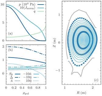
Figure 1: Pressure $p$, normalized surface-average toroidal current density $\langle J_{\text{norm}}\rangle$, and safety factor $q$ (a); fitted coefficients $S_{0}$, $\hat{\Delta}$, $\hat{\kappa}$, $\check{\kappa}$, $\hat{\eta}$, and $\check{\eta}$ (b); numerical magnetic surfaces [(c), solid lines] and analytical ones [(c), large dots]; vessel outline from reference Streibl et al., 2003.

IV Model accuracy and limitations

Whenever numerical solutions of the GS equation are replaced by analytical equilibrium models, because the former are not available or its use is not convenient, then it is necessary to understand the limitations of the latter and also which equilibrium features are retained in the simplified description. In this section, the ability of the model (15) to describe experimentally relevant scenarios is illustrated with a numerical equilibrium computed by HELENA Huysmans et al. (1991) for parameters typical of ASDEX-Upgrade operation Streibl et al. (2003). The plasma profiles are

$$\frac{dp}{d\Psi}=-1.73\times 10^{6}(1-\psi)^{3},\quad F\frac{dF}{d\Psi}=2.13\,(1-4\psi)(1-\psi),$$ (25)

both in SI units, and the boundary shape is devised in order to fit the vessel. Other parameters are the total current $I_{\text{p}}=1\,\text{MA}$, $F_{\text{vac}}=3.3\,\text{Tm}$, and $\varepsilon=0.3$. The magnetic axis is at $R_{0}=1.7\,\text{m}$, where $B_{0}=1.96\,\text{T}$.

The equilibrium pressure and toroidal current-density profiles are plotted in figure 1 in terms of the radial-like variable defined as $\rho_{\text{pol}}=\sqrt{\psi}$, along with a few magnetic surfaces. For each surface, labelled by $\psi_{i}$ ($1\leqslant i\leqslant 20$), the set of pairs $r_{ij}$ and $\theta_{ij}$ ($1\leqslant j\leqslant 200$) returned by HELENA such that $\psi(r_{ij},\theta_{ij})=\psi_{i}$ is used to retrieve the geometric coefficients in the model (15) by a least-square fitting procedure. The fitted coefficients display a mild radial variation, which validates the local approach. Also, the magnetic surfaces predicted by the analytical parametrisation (18) are seen, again in figure 1, to be in good agreement with the numerical ones, showing that the latter’s geometry has been suitably captured. However, such agreement is expected to degrade as one gets closer to the separatrix, as hinted by the slight mismatch in the outermost surface caused by the limited number of harmonics ($4$ even and $4$ odd) available in equations (16). More homogeneous terms in series (12) lead to extra harmonics, but the enhanced accuracy is outweighed by the increasing complexity in analytical expressions.

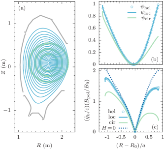
Figure 2: Magnetic surfaces from the numerical equilibrium [(a), solid lines] and from the circular model [(a), large dots]; Normalised poloidal-flux (b) and poloidal-field magnitude (c) along the midplane as predicted by the circular model, the local model (with and without the implicit dependence conveyed by $H$), and as computed by HELENA.

An equilibrium model widely adopted for analytical work has toroidal magnetic surfaces with circular and concentric section, for which the field components are Lapillonne et al. (2009)

$$B^{r}=0,\quad B^{\theta}=\frac{B_{0}}{\tilde{q}_{\text{b}}rR}\frac{d\psi}{dr},\quad B_{\phi}=R_{0}B_{0},$$ (26)

the radial poloidal flux follows the differential equation

$$\frac{d\psi}{dr}=\frac{\tilde{q}_{\text{b}}}{q(r)}\frac{r}{\sqrt{1-\varepsilon^{2}r^{2}}},$$ (27)

and $q(r)$ is the safety factor. Its limitations are evident in figure 2, where the circular surfaces are seen to depart considerably from the numerical ones. Matching $q(r)$ to the safety factor computed by HELENA along the low-field side of the midplane allows equation (27) to be solved for the poloidal flux, which is also plotted and seen to deviate from the numerical results. In stark contrast, the predictions from the local model (15) closely follow HELENA’s output regarding the poloidal flux and the poloidal-field magnitude defined as $B_{\text{pol}}^{2}=B_{r}B^{r}+B_{\theta}B^{\theta}$. Models with locally adjustable coefficients are more flexible to capture local equilibrium features than global solutions like the circular model, as figure 2 illustrates. Yet, such ability requires geometric-coefficient variations across magnetic surfaces to be taken into account, as proposed in earlier models Miller et al. (1998); Yu et al. (2012). Here, this contribution is accounted for by the factor $H$ in definition (21) and the needed derivatives are evaluated as finite differences between coefficient values fitted on adjacent surfaces.

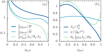
Figure 3: Asymptotic limits for the size $\bigl{|}\Delta\rho_{\text{pol}}\bigr{|}$ of the local model validity domain (a) and radial profile of the covariant toroidal current density and its partial derivative (b).

The magnitude of $H$ also places a limit on the size $\bigl{|}\Delta\psi\bigr{|}$ of the region around a surface $\psi_{i}$ where the model (15) with constant coefficients is valid, the condition being

$$\bigl{|}H\psi_{i}^{-1}\,\Delta\psi\bigr{|}=\bigl{|}2H\rho_{\text{pol}}^{-1}\,\Delta\rho_{\text{pol}}\bigr{|}\ll 1.$$ (28)

The value $H$ can be related with the derivative of the toroidal current density by expanding the GS equation, $J_{\phi}(R,\psi)$, and each geometric coefficient in equation (15) around $\psi_{i}$. The terms linear in $\Delta\psi$ yield the relation

$$-\Delta\psi\>\partial_{\Psi}\mu_{0}J_{\phi}\bigl{(}R,\psi_{i}\bigr{)}=R\nabla\cdot\bigl{(}R^{-1}\nabla H\Delta\psi\bigr{)}\sim\frac{4\widetilde{H}\Delta\psi}{a^{2}r^{2}},$$ (29)

whence the lowest-order estimate

$$\widetilde{H}\sim\tilde{q}_{\text{b}}r^{2}\>\partial_{\psi}\frac{\mu_{0}J_{\phi}(R,\psi_{i})}{4B_{0}}.$$ (30)

Figure 3 displays the asymptotic limits of the size $\bigl{|}\Delta\rho_{\text{pol}}\bigr{|}$ set by conditions (11) and (28), the latter using $H$ from equation (21) and, alternatively, $\widetilde{H}$ from estimate (30). The former condition produces very small values near the edge ($\rho_{\text{pol}}\gtrsim 0.8$) because it is proportional to $J_{\phi}$, which approaches zero there. Conversely, the condition that depends on $\widetilde{H}$, and thus on the dimensionless derivative $\partial_{\psi}\tfrac{1}{4}B_{0}^{-1}\mu_{0}J_{\phi}$ is more robust. Still, both predict smaller sizes than those found with a numerically evaluated $H$. The reason lies in the homogeneous solutions that are kept in the model (15) and its derivatives, but not in equations (11) and (30) because $R\nabla\cdot\bigl{(}R^{-1}\nabla\psi_{\text{h}}\bigr{)}=0$. The partial derivative of the toroidal current-density and the ratio $\psi/(\tilde{q}_{\text{b}}r^{2})$, both plotted in figure 3, have the same order for the equilibrium considered here and keep $\widetilde{H}\sim\psi$, which may not be true in more general cases. Equilibria with larger $J_{\phi}$ variations require a smaller $\bigl{|}\Delta\rho_{\text{pol}}\bigr{|}$ around such locations, but this does not prevent the local model (15) to apply elsewhere over the plasma cross section with more favourable validity domains.

V Analytical applications

Straight-field coordinates $\bigl{(}\psi,\chi,\phi\bigr{)}$, where the poloidal angle $\chi(r,\theta)$ is defined such that $\mathbf{b}=\mathbf{B}/B$ follows

$$b^{\phi}=q(\psi)b^{\chi},$$ (31)

are a key element in many MHD stability codes Mikhailovskii et al. (1997); Kerner et al. (1998); Mikhailovskii (1998). Usually, $\chi(r,\theta)$ is computed from numeric equilibria, but its analytical evaluation brings insight on how geometric coefficients affect $k_{\parallel}=\mathbf{k}\cdot\mathbf{b}$ and $k_{\perp}^{2}=k^{2}-k_{\parallel}^{2}$ of a MHD perturbation with $k_{\chi}=m$ and $k_{\phi}=n$. For simplicity, $H=0$ is assumed henceforth. Finite magnetic-shear effects are kept by expanding $q(\psi)$ around $\psi_{i}$ as

$$q(\psi)=q_{i}+q_{i}^{\prime}\bigl{(}\psi-\psi_{i}\bigr{)}+\cdots=\frac{\tilde{q}_{\text{b}}}{2S_{0}}\biggl{(}\frac{1}{\tilde{\iota}}+\xi\tilde{s}^{2}+\cdots\biggr{)},$$ (32)

with $1/\tilde{\iota}=2S_{0}\bigl{(}q_{i}/\tilde{q}_{\text{b}}\bigr{)}\bigl{(}1-s_{i}\bigr{)}$, $\xi=2\bigl{(}S_{0}/\psi_{i}\bigr{)}\bigl{(}q_{i}/\tilde{q}_{\text{b}}\bigr{)}s_{i}$, and $s_{i}=\psi_{i}q_{i}^{\prime}/q_{i}$, while the solution is sought as a power series in the small parameters $\varepsilon$ and $\xi$,

$$\chi(r,\theta)=\chi_{0}(\theta)+\xi r^{2}\>\chi_{\xi}(\theta)+\varepsilon r\>\chi_{\varepsilon}(\theta)+\cdots.$$ (33)

Replacing $b^{\chi}=b^{r}\partial_{r}\chi+b^{\theta}\partial_{\theta}\chi$ and the fields (22), (23), and (24) in definition (31) produces, after collecting the same powers of $\varepsilon$ and $\xi$, the coupled differential system

$$\begin{gathered}\Theta_{0}\chi_{0}^{\prime}=\tilde{\iota},\\ \Theta_{0}\chi_{\xi}^{\prime}-\Theta_{0}^{\prime}\chi_{\xi}=-\tilde{\iota}\Theta_{0}^{2}\chi_{0}^{\prime},\\ \Theta_{0}\chi_{\varepsilon}^{\prime}-\tfrac{1}{2}\Theta_{0}^{\prime}\chi_{\varepsilon}=\bigl{(}\Theta_{0}\cos\theta-\tfrac{3}{2}\Theta_{1}\bigr{)}\chi_{0}^{\prime}-2\tilde{\iota}\cos\theta.\end{gathered}$$ (34)

Setting the condition $\chi(r,0)=0$, the solutions are

$$\begin{gathered}\chi_{\xi}=-\tilde{\iota}\chi_{0}\Theta_{0},\\ \chi_{0}=\frac{\tilde{\iota}}{\tilde{\kappa}}\biggl{[}\arctan\frac{\check{\kappa}+\bigl{(}1-\hat{\kappa}\bigr{)}\tan\theta}{\tilde{\kappa}}-\arctan\frac{\check{\kappa}}{\tilde{\kappa}}\biggr{]},\\ \chi_{\varepsilon}=\tilde{\iota}\frac{C_{0}+C_{1}\cos\theta+S_{1}\sin\theta+C_{3}\cos 3\theta+S_{3}\sin 3\theta}{8\tilde{\kappa}^{4}\Theta_{0}},\end{gathered}$$ (35)

where $\tilde{\kappa}$ is such that $\tilde{\kappa}^{2}+\hat{\kappa}^{2}+\check{\kappa}^{2}=1$, while $\Theta_{00}=\Theta_{0}(0)$, $\Theta_{0\tfrac{\pi}{2}}=\Theta_{0}(\tfrac{\pi}{2})$, $\Theta_{10}=\Theta_{1}(0)$, and also

$$C_{0} =4\bigl{(}5\hat{\kappa}-1\bigr{)}\Theta_{00}^{2}\check{\eta}+9\bar{\kappa}^{2}\Theta_{00}\check{\kappa}-4\Theta_{00}\bigl{[}1-5\hat{\Delta}+3\hat{\eta}+\hat{\kappa}\bigl{(}1+\hat{\Delta}+9\hat{\eta}\bigr{)}\bigr{]}\check{\kappa}-12\Theta_{00}\check{\eta}\check{\kappa}^{2}-4\Theta_{10}\check{\kappa}^{3},$$ (36)

$$\tfrac{1}{3}C_{1} =-4\Theta^{2}_{00}\hat{\kappa}\check{\eta}-\bigl{[}3+8\hat{\Delta}-4\hat{\eta}-\hat{\kappa}\bigl{(}2+5\hat{\kappa}\bigr{)}-4\bigl{(}4+\hat{\kappa}\bigr{)}\hat{\kappa}\hat{\eta}\bigr{]}\check{\kappa}+4\bigl{(}2-\hat{\kappa}\bigr{)}\check{\eta}\check{\kappa}^{2}+\bigl{(}5+4\hat{\eta}\bigr{)}\check{\kappa}^{3},$$

$$\tfrac{1}{2}S_{1} =-2\Theta_{0\tfrac{\pi}{2}}^{2}\bigl{[}2+\Theta_{0\tfrac{\pi}{2}}\hat{\kappa}+3\bigl{(}\hat{\Delta}-\hat{\kappa}\hat{\eta}\bigr{)}\bigr{]}+6\bigl{[}1-\hat{\kappa}\bigl{(}4-\hat{\kappa}\bigr{)}\bigr{]}\check{\eta}\check{\kappa}+\bigl{[}5-6\bigl{(}\hat{\kappa}+\hat{\Delta}\bigr{)}+6\hat{\eta}\bigl{(}2+\hat{\kappa}\bigr{)}+4\hat{\kappa}^{2}\bigr{]}\check{\kappa}^{2}+6\check{\eta}\check{\kappa}^{3}+2\check{\kappa}^{4},$$

$$C_{3} =4\bigl{(}\Theta_{00}^{2}-3\check{\kappa}^{2}\bigr{)}\bigl{(}1-2\hat{\kappa}\bigr{)}\check{\eta}+4\bigl{(}1+\hat{\Delta}\bigr{)}\check{\kappa}-\bigl{(}6-9\hat{\kappa}-4\hat{\Delta}+8\hat{\eta}\bigr{)}\check{\kappa}^{3}-\bigl{[}7+16\hat{\Delta}+\hat{\kappa}\bigl{(}2-9\hat{\kappa}-4\hat{\Delta}-24\hat{\eta}\bigr{)}\bigr{]}\hat{\kappa}\check{\kappa},$$

$$S_{3} =-4\Theta^{2}_{0\tfrac{\pi}{2}}\bigl{[}\hat{\eta}+\hat{\kappa}\bigl{(}\Theta_{00}+\hat{\Delta}+2\hat{\eta}\bigr{)}\bigr{]}-24\hat{\kappa}^{2}\check{\eta}\check{\kappa}-\bigl{[}3+8\hat{\Delta}-12\hat{\eta}-\hat{\kappa}\bigl{(}8+\hat{\kappa}-4\hat{\Delta}+24\hat{\eta}\bigr{)}\bigr{]}\check{\kappa}^{2}+8\check{\eta}\check{\kappa}^{3}+5\check{\kappa}^{4}.$$

If all geometric coefficients except $S_{0}$ are set to zero, one finds the simplified transformation

$$\chi(r,\theta)=\tilde{\iota}\bigl{(}1-\tilde{\iota}\>\xi r^{2}\bigr{)}\theta-\tilde{\iota}\>\varepsilon r\sin\theta+\cdots$$ (37)

that reduces to previous results obtained in the circular limit and without magnetic shear ($\xi=0$ and $\tilde{\iota}=1$) Lapillonne et al. (2009).

The lowest order terms of $k_{\parallel}=mb^{\chi}+nb^{\phi}$ are thus

$$k_{\parallel}R_{0}=\frac{m+nq}{q_{i}\bigl{(}1-s_{i}\bigr{)}}\biggl{(}1-\varepsilon r\cos\theta-\xi\tilde{\iota}r^{2}\Theta_{0}+\cdots\biggr{)},$$ (38)

whose dependence on $\hat{\kappa}$ and $\check{\kappa}$ via $\Theta_{0}$ is rather weak for low magnetic shear ($\xi\sim s_{i}\ll 1$). The expression for $k_{\perp}$ is too complex in practice, but its linearisation around the limit of very small $\hat{\kappa}$, $\check{\kappa}$, $\hat{\eta}$, and $\check{\eta}$ yields

$$k_{\perp}\frac{ar}{\tilde{\iota}m}=1-\hat{\kappa}\cos 2\theta-\check{\kappa}\sin 2\theta-\xi\tilde{\iota}r^{2}\bigl{(}1+\theta\dot{\Theta}_{0}\bigr{)}\\ +\tfrac{3}{4}\varepsilon r\hat{\Delta}\Bigl{[}\hat{\kappa}\bigl{(}\cos 3\theta+\cos\theta\bigr{)}+\check{\kappa}\bigl{(}\sin 3\theta+\sin\theta\bigr{)}\Bigr{]}\\ -\varepsilon r\Bigl{[}\bigl{(}1-\hat{\kappa}\bigr{)}\cos\theta+\tfrac{3}{2}\Theta_{1}-\check{\kappa}\sin\theta\Bigr{]}+\cdots.$$ (39)

Unlike $k_{\parallel}$, $k_{\perp}$ depends strongly on $\hat{\kappa}$ and $\check{\kappa}$, even if $\xi\ll 1$. First-order terms in $\varepsilon$ enhance these dependencies, couple them with $\hat{\Delta}$, and connect also with $\hat{\eta}$ and $\check{\eta}$ via $\Theta_{1}$.

VI Conclusions

In summary, a local magnetic-equilibrium model with up-down asymmetric cross section was developed, where the poloidal-field flux is expanded as a series of Solovev solutions with radially changing coefficients. The model is accurate to fourth-order terms in the inverse aspect ratio and depends on eight free parameters, one for each independent poloidal-angle harmonic (five even and three odd), of which three were shown to relate with the conventional definitions of Shafranov shift, elongation, and triangularity.

In contrast with other local equilibrium models, the proposed approach was devised to produce analytically tractable expressions for the magnetic-field components. Despite such requirement, the corresponding magnetic-surface parametrisation was seen to describe equilibrium shapes, poloidal flux distributions, and magnetic-field configurations typically found in tokamak experiments. A size estimate of the domain where a local solution with constant geometric coefficients is valid was provided in terms of the local toroidal current-density derivative.

As an example of analytical application, the transformation to straight-field coordinates was obtained, up to first-order terms in the inverse aspect ratio and in the normalised magnetic shear, and then used to understand how the values $k_{\parallel}$ and $k_{\perp}$ of a MHD perturbation depend on equilibrium geometry. The suitability of the proposed local model to assess equilibrium-shaping effects, as illustrated in the examples provided, is expected to afford useful analytical insight into a wide variety of tokamak-plasma phenomena.

References

- Connor et al. (1978) J. W. Connor, R. J. Hastie, and J. B. Taylor, Phys. Rev. Lett. 40, 396 (1978).
- Greene and Chance (1981) J. Greene and M. Chance, Nucl. Fusion 21, 453 (1981).
- Bishop (1986) C. Bishop, Nucl. Fusion 26, 1063 (1986).
- Fu and Dam (1989) G. Y. Fu and J. W. V. Dam, Phys. Fluids B 1, 1949 (1989).
- Candy et al. (1996) J. Candy, B. Breizman, J. V. Dam, and T. Ozeki, Phys. Lett. A 215, 299 (1996).
- Berk et al. (2001) H. L. Berk, D. N. Borba, B. N. Breizman, S. D. Pinches, and S. E. Sharapov, Phys. Rev. Lett. 87, 185002 (2001).
- Rosenbluth and Hinton (1998) M. N. Rosenbluth and F. L. Hinton, Phys. Rev. Lett. 80, 724 (1998).
- Hinton and Rosenbluth (1999) F. L. Hinton and M. N. Rosenbluth, Plasma Phys. Control. Fusion 41, A653 (1999).
- Wong et al. (1995) H. Wong, H. Berk, and B. Breizman, Nucl. Fusion 35, 1721 (1995).
- Roach et al. (1995) C. M. Roach, J. W. Connor, and S. Janjua, Plasma Phys. Control. Fusion 37, 679 (1995).
- Brizard (2011) A. J. Brizard, Phys. Plasmas 18, 022508 (2011).
- Dorland et al. (2000) W. Dorland, F. Jenko, M. Kotschenreuther, and B. N. Rogers, Phys. Rev. Lett. 85, 5579 (2000).
- Jenko et al. (2000) F. Jenko, W. Dorland, M. Kotschenreuther, and B. N. Rogers, Phys. Plasmas 7, 1904 (2000).
- Candy and Waltz (2003) J. Candy and R. Waltz, J. Comput. Phys. 186, 545 (2003).
- Peeters et al. (2009) A. Peeters, Y. Camenen, F. Casson, W. Hornsby, A. Snodin, D. Strintzi, and G. Szepesi, Comp. Phys. Comm. 180, 2650 (2009).
- Beer et al. (1995) M. A. Beer, S. C. Cowley, and G. W. Hammett, Phys. Plasmas 2, 2687 (1995).
- Hegna (2000) C. C. Hegna, Phys. Plasmas 7, 3921 (2000).
- Miller et al. (1998) R. L. Miller, M. S. Chu, J. M. Greene, Y. R. Lin-Liu, and R. E. Waltz, Phys. Plasmas 5, 973 (1998).
- Zhou and Yu (2011) D. Zhou and W. Yu, Phys. Plasmas 18, 052505 (2011).
- Solovev (1968) L. S. Solovev, Sov. Phys. JETP 26, 400 (1968).
- Cerfon and Freidberg (2010) A. J. Cerfon and J. P. Freidberg, Phys. Plasmas 17, 032502 (2010).
- Zheng et al. (1996) S. B. Zheng, A. J. Wootton, and E. R. Solano, Phys. Plasmas 3, 1176 (1996).
- Rodrigues and Bizarro (2004) P. Rodrigues and J. P. S. Bizarro, Phys. Plasmas 11, 186 (2004).
- Rodrigues and Bizarro (2009) P. Rodrigues and J. P. S. Bizarro, Phys. Plasmas 16, 022505 (2009).
- Rodrigues et al. (2014) P. Rodrigues, N. F. Loureiro, J. Ball, and F. I. Parra, Nucl. Fusion 54, 093003 (2014).
- Ball et al. (2014) J. Ball, F. I. Parra, M. Barnes, W. Dorland, G. W. Hammett, P. Rodrigues, and N. F. Loureiro, Plasma Phys. Control. Fusion 56, 095014 (2014).
- Yu et al. (2012) W. Yu, D. Zhou, and N. Xiang, Phys. Plasmas 19, 072520 (2012).
- Streibl et al. (2003) B. Streibl, P. T. Lang, F. Leuterer, J.-M. Noterdaeme, and A. Stäbler, Fusion Sci. Technol. 44, 578 (2003).
- Huysmans et al. (1991) G. Huysmans, J. Goedbloed, and W. Kerner, Int. J. Mod. Phys. C 2, 371 (1991).
- Lapillonne et al. (2009) X. Lapillonne, S. Brunner, T. Dannert, S. Jolliet, A. Marinoni, L. Villard, T. Görler, F. Jenko, and F. Merz, Phys. Plasmas 16, 032308 (2009).
- Mikhailovskii et al. (1997) A. B. Mikhailovskii, G. T. A. Huysmans, W. O. K. Kerner, and S. E. Sharapov, Plasma Phys. Rep. 23, 844 (1997).
- Kerner et al. (1998) W. Kerner, J. Goedbloed, G. Huysmans, S. Poedts, and E. Schwarz, J. Comput. Phys. 142, 271 (1998).
- Mikhailovskii (1998) A. B. Mikhailovskii, Plasma Phys. Control. Fusion 40, 1907 (1998).