Discrete-Event Continuous-Time Recurrent Nets

Abstract

We investigate recurrent neural network architectures for event-sequence processing. Event sequences, characterized by discrete observations stamped with continuous-valued times of occurrence, are challenging due to the potentially wide dynamic range of relevant time scales as well as interactions between time scales. We describe four forms of inductive bias that should benefit architectures for event sequences: temporal locality, position and scale homogeneity, and scale interdependence. We extend the popular gated recurrent unit (GRU) architecture to incorporate these biases via intrinsic temporal dynamics, obtaining a continuous-time GRU. The CT-GRU arises by interpreting the gates of a GRU as selecting a time scale of memory, and the CT-GRU generalizes the GRU by incorporating multiple time scales of memory and performing context-dependent selection of time scales for information storage and retrieval. Event time-stamps drive decay dynamics of the CT-GRU, whereas they serve as generic additional inputs to the GRU. Despite the very different manner in which the two models consider time, their performance on eleven data sets we examined is essentially identical. Our surprising results point both to the robustness of GRU and LSTM architectures for handling continuous time, and to the potency of incorporating continuous dynamics into neural architectures.

1 Introduction

Many classic data sources in machine learning can be characterized as sequences. For example, natural language text is a progression of words; videos consist of a series of still images; and spoken utterances are represented as sampled power spectra. In such sequences, observations are ordered but there is no timing information. In contrast to these ordinal sequences, event sequences consist of observations stamped with a continuous-valued, absolute or relative time of occurrence. Examples of event sequences include online product purchases, criminal activity in a police blotter, web forum postings, an individual’s restaurant reservations, file accesses, outgoing phone calls or text messages, sent emails, player log-ins to gaming sites, and music selections. In each of these examples, discrete events occur in continuous time and not necessarily at uniform intervals.

In this article, we focus on recurrent neural net (RNN) approaches to processing event sequences. We consider standard tasks for event sequences that include classification, prediction of the next event given the time lag from the previous event, and prediction of the time lag to the next event.

Existing sequence learning methods for recurrent nets, e.g., LSTM (Hochreiter and Schmidhuber, 1997) and GRU (Chung et al., 2014) architectures, are not designed for event sequences but might be extended to handle them in various ways. First, time stamps might simply be ignored (e.g., Wu et al., 2016). Second, time might be discretized, allowing an event-based sequence to be transformed into a sequence sampled at fixed clock intervals (e.g., Hidasi et al., 2015; Song et al., 2016; Wang et al., 2016a; Wu et al., 2017). Third, time stamps might be used as additional input features (e.g., Choi et al., 2016; Du et al., 2016). We explore the hypothesis that time should be handled in a more specialized manner.

To explain what we mean by ‘specialized,’ consider the deep learning architecture universally used for vision—the convolutional network (Fukushima, 1980; Lecun et al., 1998; Mozer, 1987). Convolutional nets are successful because they incorporate three forms of inductive bias: (1) spatial locality—features at nearby locations in an image are more likely to have joint causes and consequences than more distant features; (2) spatial position homogeneity—features deemed significant in one region of an image are likely to be significant in other regions; and (3) spatial scale homogeneity—spatial locality and position homogeneity should apply across a range of spatial scales.

Architectures for event sequences should benefit from isomorphic forms of inductive bias, specifically: (1) temporal locality—events closer in time are more likely to have joint causes and consequences than more distant events; (2) temporal position homogeneity—event patterns deemed significant at one point in time are likely to be significant at other points; and (3) temporal scale homogeneity—temporal locality and position homogeneity should apply across a range of time scales.

We examine event-sequence architectures that incorporate these biases, plus one more: (4) temporal scale interactions—sequences have different structure at different scales and these scales interact. Scale interactions are also found in vision, and models have been designed to leverage these interactions by incorporating multi-resolution pyramids at every stage of a convolutional architecture (e.g., Buyssens et al., 2013; Zeng et al., 2017). To illustrate interactions across temporal scales, consider the scenario of online shopping. A customer may browse various TV models one week, home automation devices the next, and phones the next. Each of these activity patterns indicates at least a short-term interest in some topic, but the combination of the searches indicates a long-term interest in electronics. On the flip side, customers may frantically shop for parts when their furnace fails, but that does not imply a long-term interest in furnace paraphernalia—contrary to the annoying inference that shopping sites appear to make.

1.1 Existing approaches to event-sequence learning

We believe that event-sequence learning can be improved because existing techniques fall short in incorporating the four biases we listed. For example, one standard technique is to include time stamps as additional inputs; these inputs gives deep learning models in principle all the necessary flexibility to handle time. However, the flexibility may simply be too great, in the same way that fully connected deep nets are too flexible to match convolutional net performance in vision tasks (Lecun et al., 1998). The architectural biases serve to constrain learning in a helpful manner.

Given the similarity between the spatial regularities incorporated into the convolutional net and the temporal regularities we described, it seems natural to use a convolutional architecture for sequences, essentially remapping time into space (Waibel et al., 1990; Lockett and Miikkulainen, 2009; Nguyen et al., 2016; Taylor et al., 2010; Kalchbrenner et al., 2014; Sainath et al., 2015; Zeng et al., 2016). In terms of the biases that we conjecture to be helpful, convolutional nets can check all the boxes, and some recent work has begun to investigate multiscale convolutional nets for time series to capture scale interactions (Cui et al., 2016). However, convolutional architectures poorly address the continuous nature of time and the potential wide range of time scales. Consider a domain such as network intrusion detection: event patterns of relevance can occur on a time scale of microseconds to weeks (Mukherjee et al., 1994; Palanivel and Duraiswamy, 2014). It is difficult to conceive how a convolutional architecture could accommodate this dynamic range.

RNN architectures have been proposed to address the multiscale nature of time series and to handle interactions of temporal scale, but these approaches have been focused on ordinal sequences and indexing is based on sequence position rather than chronological time. This work includes clockwork RNNs (Koutník et al., 2014), gated feedback RNNs (Chung et al., 2015), and hierarchical multiscale RNNs (Chung et al., 2016).

A wide range of probabilistic methods have been applied to event sequences, including hidden semi-Markov models and survival analysis (Kapoor et al., 2014, 2015; Zhang et al., 2016), temporal point processes (Dai et al., 2016; Du et al., 2015, 2016; Wang et al., 2016b), nonstationary bandits (Komiyama and Qin, 2014), and time-sensitive latent-factor models (Koren, 2010). All probabilistic methods properly treat chronological time as time, and therefore naturally incorporate temporal locality and position homogeneity biases. These methods also tend to permit a wide dynamic range of time scales. However, they are limited by strong generative assumptions. Our aim is to combine the strength of probabilistic methods—having an explicit theory of temporal dynamics—with the strength of deep learning—having the ability to discover representations.

2 Continuous-time recurrent networks

All dynamical event-sequence models must construct memories that encapsulate information from past that is relevant for future prediction, action, or classification. This information may have a limited lifetime of utility, and stale information which is no longer relevant should be forgotten. LSTM (Hochreiter and Schmidhuber, 1997) was originally designed to operate without forgetting, but adding a mechanism of forgetting improved the architecture (Gers et al., 2000). The intrinsic dynamics of the newer GRU (Chung et al., 2014) architecture incorporates forgetting: storage of new information is balanced against the forgetting of old.

In this section, we summarize the GRU architecture and we characterize its forgetting mechanism from a novel perspective that facilitates generalizing the architecture to handling sequences in continuous time. For exposition’s sake, we present our approach in terms of the GRU, but it could be cast in terms of LSTM just as well. There appears to be no functional difference between the two architectures with proper initialization (Jozefowicz et al., 2015).

2.1 Gated recurrent unit (GRU)

The most basic architecture using gated-recurrent units (GRUs) involves an input layer, a recurrent hidden GRU layer, and an output layer. A schematic of the GRU units is shown in the left panel of Figure 1. The reset gate, ${\bm{r}}$, shunts the activation of the previous hidden state, ${\bm{h}}$. The shunted state, in conjunction with the external input, ${\bm{x}}$, is used to detect the presence of task-relevant events (${\bm{q}}$). The update gate, ${\bm{s}}$, then determines what proportion of the old hidden state should be retained and what proportion of the detected event should be stored. Formally, given an external input ${\bm{x}}_{k}$ at step $k$ and the previous hidden state ${\bm{h}}_{k-1}$, the GRU layer updates as follows:

1. Determine reset gate settings	${\bm{r}}_{k}\leftarrow\mathrm{logistic}({\bm{W}}^{\scriptscriptstyle R}{\bm{x}}_{k}+{\bm{U}}^{\scriptscriptstyle R}{\bm{h}}_{k-1}+{\bm{b}}^{\scriptscriptstyle R})$
2. Detect relevant event signals	${\bm{q}}_{k}\leftarrow\mathrm{tanh}({\bm{W}}^{\scriptscriptstyle Q}{\bm{x}}_{k}+{\bm{U}}^{\scriptscriptstyle Q}({\bm{r}}_{k}\circ{\bm{h}}_{k-1})+{\bm{b}}^{\scriptscriptstyle Q})$
3. Determine update gate settings	${\bm{s}}_{k}\leftarrow\mathrm{logistic}({\bm{W}}^{\scriptscriptstyle S}{\bm{x}}_{k}+{\bm{U}}^{\scriptscriptstyle S}{\bm{h}}_{k-1}+{\bm{b}}^{\scriptscriptstyle S})$
4. Update hidden state	${\bm{h}}_{k}\leftarrow(1-{\bm{s}}_{k})\circ{\bm{h}}_{k-1}+{\bm{s}}_{k}\circ{\bm{q}}_{k}$

where ${\bm{W}}^{*}$, ${\bm{U}}^{*}$, and ${\bm{b}}^{*}$ are model parameters, $\circ$ denotes the Hadamard product, and ${\bm{h}}_{0}=\bm{0}$.

Figure 1: A schematic of the GRU (left) and CT-GRU (right). Color coding of the elements matches the background color used in the tables presenting activation dynamics. For the CT-GRU, the large rectangle with segments represents a multiscale hidden representation. The intrinsic decay temporal decay of this representation, as well as the recurrent self-connections, is not depicted in the schematic.

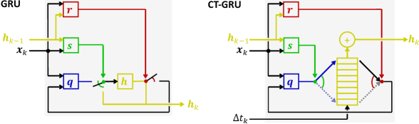
Readers who are familiar with GRUs may notice that our depiction of GRUs in in Figure 1 looks a bit different than the depiction in the originating article (Chung et al., 2014). Our intention is to highlight the fact that the ‘update’ gate is actually making a decision about what to store in the memory (hence the notation ${\bm{s}}$), and the ‘reset’ gate is actually making a decision about what to retrieve from the memory (hence the notation ${\bm{r}}$). The schematic in Figure 1 makes obvious the store and retrieval operations via the gate placement on the input to and output from the hidden state, ${\bm{h}}$, respectively.

To incorporate time into the GRU, we observe that the storage operation essentially splits each new event, ${\bm{q}}_{k}$, into a portion ${\bm{s}}_{k}$ that is stored indefinitely and a portion $1-{\bm{s}}_{k}$ that is stored for only an infinitesimally short period of time. Similarly, the retrieval operation reassembles a memory by taking a proportion, ${\bm{r}}_{k}$, of a long-lasting memory—via the product ${\bm{r}}_{k}\circ{\bm{h}}_{k-1}$—and a complementary proportion, $1-{\bm{r}}_{k}$ of a very very short-term memory—a memory so brief that it has decayed to $\bm{0}$. The retrieval operation is thus equivalent to computing the mixture ${\bm{r}}_{k}\circ{\bm{h}}_{k-1}+(1-{\bm{r}}_{k})\circ\bm{0}$.

The essential idea of the model we will introduce, the CT-GRU, is to endow each hidden unit with multiple memory traces that span a range of time scales, in contrast to the GRU which can be conceived of as having just two time scales: one infinitely long and one infinitesimally short. We define time scale in the standard sense of a linear time-invariant system, operating according to the differential equation $dh/dt=-h/\tau$, where $h$ is the memory, $t$ is continuous time, and $\tau$ is a (nonnegative) time constant or time scale. These dynamics yield exponential decay, i.e., $h(t)=e^{-t/\tau}h(0)$ and $\tau$ is the time for the state to decay to a proportion $e^{-1}\approx.37$ of its initial level. The short and long time scales of the GRU correspond to the limits $\tau\to 0$ and $\tau\to\infty$, respectively.

2.2 Continuous-time gated recurrent unit (CT-GRU)

We argued that the storage (or update) gate of the GRU decides how to distribute the memory of a new event across time scales, and the retrieval (or reset) gate decides how to collect information previously stored across time scales. Binding memory operations to a time scale is sensible for any intelligent agent because different activities require different memory durations. To use human cognition as an example, when you are told a phone number, you need remember it only for a few seconds to enter it in your phone; when making a mental shopping list, you need remember the items only until you get to the store; but when a colleague goes on sabbatical and returns a year later, you should still remember her name. Although individuals typically do not wish to forget, forgetting can be viewed as adaptive (Anderson and Milson, 1989): when information becomes stale or is no longer relevant, it only interferes with ongoing processing and clutters memory. Indeed, cognitive scientists have shown that when an attribute must be updated frequently in memory, its current value decays more rapidly (Altmann and Gray, 2002). This phenomenon is related to the benefit of distributed practice on human knowledge retention: when study is spaced versus massed in time, memories are more durable (Mozer et al., 2009).

Returning to the CT-GRU, our goal is to develop a model that—consistent with the GRU—stores each new event at a time scale deemed appropriate for it, and similarly retrieves information from an appropriate time scale. Thus, we wish to replace the GRU storage and retrieval gates with storage and retrieval scales, computed from the external input and the current hidden state. The scale is expressed in terms of a time constant.

To store event $k$ at an arbitrary scale $\tau_{k}^{\scriptscriptstyle S}$ (the superscript $s$ denotes ‘storage’), each would require a separate trace. Because separate traces are not feasible, we propose instead a fixed set of traces with predefined time scales, and each to-be-stored event is distributed among the available traces. Specifically, we propose a fixed set of $M$ traces with log-linear spaced time scales, ${\smash{\tilde{T}}}\equiv\{{\tilde{\tau}}_{1},{\tilde{\tau}}_{2},\ldots{\tilde{\tau}}_{M}\}$, and we approximate the storage of a single trace at scale $\tau_{k}^{\scriptscriptstyle S}$ with a mixture of traces from ${\smash{\tilde{T}}}$. Of course, an exponential curve with an arbitrary decay rate cannot necessarily be modeled as a mixture of exponentials with predefined decay rates. However, we can attempt to ensure that the half life of the mixture matches the half life of the target. Through experimentation, we have achieved a match with high fidelity when $s_{ki}$, the proportion of the to-be-stored signal allocated to fixed scale $i$, is:

$$\textstyle{s_{ki}\leftarrow{e^{-[\ln({\tilde{\tau}}_{i}/\tau_{k}^{\scriptscriptstyle S})]^{2}}}/{\sum_{j}e^{-[\ln({\tilde{\tau}}_{j}/\tau_{k}^{\scriptscriptstyle S})]^{2}}}}.$$ (1)

Figure 2: (a) Half life for a range of time scales: true value (dashed black line) and mixture approximation (blue line). (b) Decay curves for time scales $\tau\in[10,100]$ (solid lines) and the mixture approximation (dashed lines).

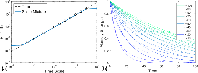
Figure 2a shows that the half life of arbitrary time scales can be well approximated by a finite mixture of time scales. The graph plots half life as a function of time scale, with the veridical mapping shown as a dashed black line, and the approximation shown as the solid blue line for ${\smash{\tilde{T}}}$ consisting of the open circles on the graph. Obviously, one cannot extrapolate to time scales outside the range in ${\smash{\tilde{T}}}$, but enough should be known about a problem domain to determine a bounding range of time scales. We have found that constraining separation among constants in ${\smash{\tilde{T}}}$ such that ${\tilde{\tau}}_{i+1}=10^{1/2}{\tilde{\tau}}_{i}$ achieves a high-fidelity match. Figure 2b plots memory decay as a function of time for time scales $\{10,20,\ldots,100\}$ (solid lines), along with the mixture approximation (dashed lines) using the set of scales in Figure 2a. Corresponding solid and dashed curves match well in their half lives (open circles), despite the fact that the approximation is more like a power function, with faster decay early on and slower decay later on. The heavy tails should, if anything, be helpful for preserving state and error gradients. For the sake of modeling, the important point is that a continuous change in $\tau_{k}^{\scriptscriptstyle S}$ produces continuous changes in both the weightings $s_{ki}$ and the effective decay function.

Just as the GRU determines the position of the storage (update) gate from its input, the CT-GRU determines the time scale of storage, $\tau_{k}^{\scriptscriptstyle S}$. We use an exponential transform to ensure nonnegative $\tau_{k}^{\scriptscriptstyle S}$:

$${\bm{\tau}}_{k}^{{\scriptscriptstyle S}}\leftarrow\exp\left({\bm{W}}^{\scriptscriptstyle S}{\bm{x}}_{k}+{\bm{U}}^{\scriptscriptstyle S}{\bm{h}}_{k-1}+{\bm{b}}^{\scriptscriptstyle S}\right).$$ (2)

Functionally, the $\{s_{ki}\}$ derived from $\tau_{k}^{\scriptscriptstyle S}$ serve as gates on each of the fixed-scale traces. The retrieval operation mirrors the storage operation. A time scale of retrieval, $\tau_{k}^{\scriptscriptstyle R}$ is computed from the input, and a half-life-matching mixture of the stored traces serves as the retrieved value from the CT-GRU memory. The right panel of Figure 1 shows a schematic of the CT-GRU with ${\bm{s}}$ and ${\bm{r}}$ used to select the storage and retrieval scales from a multiscale memory trace. The time lag between events, $\Delta t_{k}$, is an explicit input to the memory, used to determine the amount of decay between discrete events. The CT-GRU and GRU updates are composed of the identical steps, and in fact the CT-GRU with just two scales, ${\smash{\tilde{T}}}=\{0,\infty\}$, and fixed $\Delta t_{k}$, is identical to the GRU. The dynamics of storage and retrieval simplify because the logarithmic term in Equation 1 cancels with the exponentiation in Equation 2, yielding the elegant CT-GRU update:

1. Determine retrieval scale and weighting	$\ln{\bm{\tau}}_{k}^{\scriptscriptstyle R}\leftarrow{\bm{W}}^{\scriptscriptstyle R}{\bm{x}}_{k}+{\bm{U}}^{\scriptscriptstyle R}{\bm{h}}_{k-1}+{\bm{b}}^{\scriptscriptstyle R}$ ${\bm{r}}_{ki}\leftarrow\mathrm{softmax}_{i}\left(-(\ln{\bm{\tau}}_{k}^{\scriptscriptstyle R}-\ln{\tilde{\tau}}_{i})^{2}\right)$
2. Detect relevant event signals	${\bm{q}}_{k}\leftarrow\mathrm{tanh}({\bm{W}}^{\scriptscriptstyle Q}{\bm{x}}_{k}+{\bm{U}}^{\scriptscriptstyle Q}(\sum_{i}{\bm{r}}_{ki}\circ{\hat{\bm{h}}}_{k-1,i})+{\bm{b}}^{\scriptscriptstyle Q})$
3. Determine storage scale and weighting	$\ln{\bm{\tau}}_{k}^{\scriptscriptstyle S}\leftarrow{\bm{W}}^{\scriptscriptstyle S}{\bm{x}}_{k}+{\bm{U}}^{\scriptscriptstyle S}{\bm{h}}_{k-1}+{\bm{b}}^{\scriptscriptstyle S}$ ${\bm{s}}_{ki}\leftarrow\mathrm{softmax}_{i}\left(-(\ln{\bm{\tau}}_{k}^{\scriptscriptstyle S}-\ln{\tilde{\tau}}_{i})^{2}\right)$
4. Update multiscale state	${\hat{\bm{h}}}_{ki}\leftarrow\left[(1-{\bm{s}}_{ki})\circ{\hat{\bm{h}}}_{k-1,i}+{\bm{s}}_{ki}\circ{\bm{q}}_{k}\right]e^{-\Delta t_{k}/{\tilde{\tau}}_{i}}$
5. Combine time scales	${\bm{h}}_{k}\leftarrow\sum_{i}{\hat{\bm{h}}}_{ki}$

3 Experiments

We compare the CT-GRU to a standard GRU that receives additional real-valued $\Delta t$ inputs. Although the CT-GRU is derived from the GRU, the CT-GRU is wired with a specific form of continuous time dynamics, whereas the GRU is free to use the $\Delta t$ input in an arbitrary manner. The conjecture that motivated our work is that the inductive bias built into the CT-GRU would enable it to better leverage temporal information and therefore outperform the overly flexible, poorly constrained GRU.

We have conducted experiments on a diverse variety of event-sequence data sets, synthetic and natural. The synthetic sets were designed to reveal the types of temporal structure that each architecture could discover. We have explored a range of classification and prediction tasks. The punch line of our work is this: Although the CT-GRU and GRU handle time in very different manners, the two architectures perform essentially identically. We found almost no empirical difference between the models. Where one makes errors, the other makes the same errors. Both models perform significantly above sensible baselines, and both models leverage time, albeit in a different manner. Nonetheless, we will argue that the CT-GRU has interesting dynamics and offers lessons for future research.

3.1 Methodology

In all simulations, we present sequences of symbolic event labels. The input is a one-hot representation of the current event, $x_{k}$. For the CT-GRU, $\Delta t_{k}$—the lag between events $k$ and $k+1$—is provided as a special input that modulates decay (see Figure 1b). For the GRU, $\Delta t_{k-1}$ and $\Delta t_{k}$ are included as standard real-valued inputs. The output layer representation and activation function depends on the task. For event-label prediction, the task is to predict the next event, $x_{k+1}$; the output layer is a one-hot representation with a softmax activation function. For event-polarity prediction, the task is to predict a binary property of the next event. For this task, the output consists of one logistic unit per event label; only the event that actually occurs is provided a target ($0$ or $1$) value. For classification, the task is to map a complete sequence to one of two classes, $0$ or $1$, via a logistic output unit.

We constructed independent Theano (Theano Development Team, 2016) and TensorFlow (Abadi et al., 2015) implementations as a means of verifying the code. For all data sets, 15% of the training set is used as validation data model selection, performed via early stopping and selection from a range of hidden layer sizes. We assess test-set performance via three measures: accuracy, log likelihood, and a discriminability measure, AUC (Green and Swets, 1966). We report accuracy because it closely mirrors log likelihood and AUC on all data sets, and accuracy is most intuitive. More details of the simulation methodology and a complete description of data sets can be found in the Supplementary Materials.

3.2 Discovery of temporal patterns in synthetic data

To illustrate the operation of the CT-GRU, we devised a Working memory task requiring limited-duration information storage. The input sequence consists of commands to store, for a duration of 1, 10, or 100 time units—specified by the commands s, m, or l—a specific symbol— a, b, or c. The input sequence also contains symbols a-c in isolation to probe memory for whether the symbol is currently stored. For example, with $\text{x}/t$ denoting event x at time $t$, consider the sequence: $\{\text{m}/0,\text{b}/0,\text{b}/5\}$. The first two events instruct the memory to store b for 10 time units. The third probes for b at time 5, which should produce a response of 1, whereas probes $\text{b}/25$ or $\text{a}/5$ should produce 0.

Figure 3: Working memory task: (a) CT-GRU (blue) and GRU (orange) response to probe on sequences like $\{\text{l}/0,\text{x}/0,\ldots,\text{x}/t\}$ for a range of $t$. (b) Storage timescales, $\log_{10}({\bm{\tau}}_{k}^{\scriptscriptstyle S})$, and event-detection weights, ${\bm{W}}^{\scriptscriptstyle Q}$. The CT-GRU modulates storage time scale of symbol based on the context.

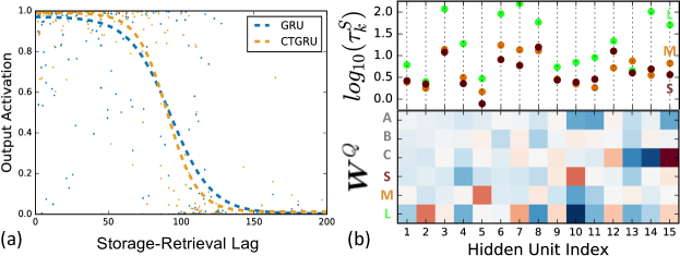
Both GRU and CT-GRU with 15 hidden units learn the task well, with 98.8% and 98.7% test-set accuracy, respectively. Figure 3a plots probe response to sequences of the form $\{\text{l}/0,\text{x}/0,\ldots,\text{x}/t\}$ for various durations $t$. The scatterplot represents individual test sequences; the dashed line is a logistic fit. Both the GRU and CT-GRU show a drop off in response around $t=100$, as desired, although the CT-GRU shows a more ideal, sharper cut off. Due to its explicit representation of time scale, the CT-GRU is amenable to dissection and interpretation. The bottom of Figure 3b shows weights ${\bm{W}}^{\scriptscriptstyle Q}$ for the fifteen CT-GRU hidden units, arranged such that the units which respond more strongly to symbols a–c—and thus will serve as memory for these symbols—are further to the right (blue negative, red positive). The top of the Figure shows the storage timescale, expressed as $\log_{10}{\bm{\tau}}_{k}^{\scriptscriptstyle S}$, for a symbol a–c when preceded by commands s, m, or l. In accordance with task demands, the CT-GRU modulates the storage time scale based on the command context.

Figure 4: Event sequences for (a) Cluster, (b) Hawkes process, and (c) Reddit. Time is on horizontal axis. Color denotes event label; in (a), irrelevant labels are rendered as dashed black lines.

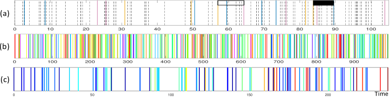
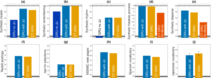
Moving on to more systematic investigations, we devised three synthetic data sets for which inter-event times are required to attain optimal performance. Data set Cluster classifies 100-element sequences according to whether three specific events occur in any order within a given time span. Figure 4a shows a sample sequence with critical elements that both satisfy and fail to satisfy the time-span requirement, indicated by the solid and outline rectangle, respectively. Remembering outputs a binary value for each event label indicating whether the lag from the last occurrence of the event is below or above a critical time threshold. Rhythm classifies 100-element sequences according to whether the inter-event timings follow a set of event-contingent rules, like a type of musical notation. The CT-GRU performs no better than the GRU with $\Delta t$ inputs, although both outperform the GRU without $\Delta t$ (Figures 5a-c), indicating that both architectures are able to use the temporal lags. For these and all other simulations reported, errors produced by the CT-GRU and the GRU are almost perfectly correlated. (Henceforth, we refer to the GRU with $\Delta t$ as the GRU.)

We ran ten replications of Cluster with different initializations and different example sequences, and found no reliable difference between CT-GRU and GRU by a two-sided Wilcoxon sign rank test ($p=.43$). Because our data sets are almost all large—with between 10k to 100k training and test examples—and because our aim is not to argue that the CT-GRU outperforms the GRU, we report outcomes from a single simulation run in Figures 5a-i.

Having demonstrated that the GRU is able to leverage the $\Delta t$ inputs, we conducted two simulations to show that the CT-GRU requires decay dynamics to achieve its performance. We created a version of the CT-GRU in which the traces did not decay with the passage of time. In principle, such an architecture could be used as a flexible memory, where a unit decides which memory slot to use for information storage and retrieval. However, in practice removing decay dynamics for intrinsically temporal tasks harms the CT-GRU (Figures 5d,e). Data set Hawkes process consists of parallel event streams generated by independent Hawkes processes operating over a range of time scales; an example sequence is shown in Figure 4b. Data set Disperse classifies event streams according to whether two specific events occur in a precise but distant temporal relationship.

Figure 5: Comparison of GRU, CT-GRU, and variants. Data sets (a)-(i) consist of at least 10k training and test examples and thus a single train/test split is adequate for evaluation. Smaller data set (j) is tested via 8-fold cross validation. Solid black lines represent a reference baseline performance level, and dashed lines indicate optimal performance (where known).

3.3 Naturalistic data sets

We experimented with five real-world event-sequence data sets, described in detail in the Supplementary Materials. Reddit is the timeseries of subreddit postings of 30k users, with sequences spanning up to several years and a thousand postings (Figure 4c). Last.fm has 300 time-tagged artist selections of 30k users, spanning a time range from hours to months. Msnbc, from the UCI repository (Lichman, 2013), has the sequence of categorized MSNBC web pages viewed in 120k sessions. Spanish and Japanese are data sets of students practicing foreign language vocabulary over a period of up to 4 months, with the lag between practice of a vocabulary item ranging from seconds to months. Reddit, Last.fm, and Msnbc are event-label prediction tasks; Spanish and Japanese require event-polarity prediction (whether students successfully translated a vocabulary item given their study history). Because students forget with the passage of time, we expected that CT-GRU would be particularly effective for modeling human memory strength.

Figures 5f-j reveal no meaningful performance difference between the GRU and CT-GRU architectures, and both architectures outperform a baseline measure (depicted as the solid black line in the Figures). For Reddit, Last.fm, and Msnbc, the baseline is obtained by predicting the next event label is the same as the current label; for Spanish and Japanese, the baseline is obtained by predicting the same success or failure for a vocabulary item as on the previous trial. Significantly beating baseline is quite difficult for each of these tasks because they involve modeling human behavior that is governed by many factors external to event history.

The most distressing result, which we do not show in the Figures, is that for each of these tasks, removing the $\Delta t$ inputs from the GRU has only a tiny impact on performance, at most a 5% drop toward baseline. Thus, neither GRU nor CT-GRU is able to leverage the timing information in the event stream. One possibility is that the stochasticity of human behavior overwhelms any signal in event timing. If so, time tags may provide more leverage for event sequences obtained from alternative sources (e.g., computer systems, physical processes). However, we are not hopeful given that our synthetic data sets also failed to show an advantage for the CT-GRU, and those data sets were crafted to benefit an architecture like CT-GRU with intrinsic temporal dynamics.

3.4 Summary of other investigations

We conducted a variety of additional investigations that we summarize here. First, we hoped that with smaller data sets, the value of the inductive bias in the CT-GRU would give it an advantage over the GRU, but it did not. Second, we tested other natural and synthetic data sets, but the pattern of results is as we report here. Third, we considered additional tasks that might reveal an advantage of the CT-GRU such as sequence extrapolation and event-timing prediction. And finally, we developed literally dozens of alternative neural net architectures that, like the CT-GRU, incorporate the forms of inductive bias described in the introduction that we expected to be helpful for event-sequence processing. All of these architectures share intrinsic time-based decay whose dynamics are modulated by information contained in the event sequence. These architectures include: variants of the CT-GRU in which the retrieved state is also used for output and computation of the storage and retrieval scales; the LSTM analog of the CT-GRU, with multiple temporal scales; and a variety of memory mechanisms whose internal dynamics are designed to mimic mean-field approximations to stochastic processes, including survival processes and self-excitatory and self-inhibitory point processes (e.g., Hawkes processes). Some of these models are easier to train than others, but, in the end, none beat the performance of generic LSTM or GRU architectures provided with additional $\Delta t$ inputs.

4 Discussion

Our work is premised on the hypothesis that event-sequence processing in RNN architectures could be improved by incorporating domain-appropriate inductive bias. Despite a concerted, year-long effort, we found no support for this hypothesis. Selling a null result is challenging. We have demonstrated that there is no trivial or pathological explanation for the null result, such as implementation issues with the CT-GRU or the possibility that both architectures simply ignore time. Our methodology is sound and careful, our simulations extensive and thorough. Nevertheless, negative results can be influential, e.g., the failure to learn long-term temporal dependencies (Hochreiter et al., 2001; Hochreiter, 1998; Bengio et al., 1994; Mozer, 1992) led to the discovery of novel RNN architectures. Further, this report may save others from a duplication of effort. We also note, somewhat cynically, that a large fraction of the novel architectures that are claimed to yield promising results one year seem to fall by the wayside a year later.

One possible explanation for our null result may come from the fact that the CT-GRU has no more free parameters than the GRU. In fact, the GRU has more parameters because the inter-event times are treated as additional inputs with associated weights in the GRU. The CT-GRU and GRU have different sorts of flexibility via their free parameters, but perhaps the space of solutions they can encode is roughly the same. Nonetheless, we are a bit mystified as to how they could admit the same solution space, given the very different manners in which they encode and utilize time.

Our work has two key insights that ought to have value for future research. First, we cast the popular LSTM and GRU architectures in terms of time-scale selection rather than in terms of gating information flow. Second, we show that a simple mechanism with a finite set of time scales is capable of storing and retrieving information from a continuous range of time scales.

To end on a more positive note, incorporating continuous-time dynamics into neural architectures has led us to some observations worthy of further pursuit. For example, consider the possibility of multiple events occurring simultaneously, e.g., a stream of outgoing emails might be coded in terms of the recipients, and a single message may be sent to multiple individuals. The state of an LSTM, GRU, or CT-GRU will depend on the order that the individuals are presented. However, we can incorporate into the CT-GRU absorption time dynamics for an input $x$, via the closed-form solution to differential equations $dh=-h/\tau_{hid}+x/\tau_{in}$ and $dx=-x/\tau_{in}$, yielding a model whose dynamics are invariant to order for simultaneous events, and relatively insensitive to order for events arriving closely in time. Such behavior could have significant benefits for event sequences with measurement noise or random factors influencing arrival times.

Acknowledgments

This research was supported by NSF grants DRL-1631428 and SES-1461535.

A

A.1 Simulation methodology

We constructed independent theano (Theano Development Team, 2016) and tensorflow (Abadi et al., 2015) implementations as a means of verifying the code. For all data sets, 15% of the training set is used as validation data model selection, performed via early stopping and selection from a range of hidden layer sizes. Optimization was performed via RMSPROP. Drop out was not used as it appeared to have little impact on results. We assessed performance on a test set via three measures: accuracy of prediction/classification, log likelihood of correct prediction/classification, and AUC (a discriminability measure) (Green and Swets, 1966). Because accuracy mirrored the other two measures for our data sets and because it is the most intuitive, we report accuracy. For event-label prediction tasks, a response is correct if the highest output probability label is the correct label. For classification tasks and event-polarity prediction tasks, a response is correct if the error magnitude is less than 0.5 for outputs in $[0,1]$.

A.1.1 GRU initialization

The GRU ${\bm{U}}^{*}$ and ${\bm{W}}^{*}$ weights are initialized with $L_{2}$ norm 1 and such that the fan-in weights across hidden units are mutually orthogonal. The GRU ${\bm{b}}^{*}$ are initialized to zero. Other weights, including the mapping from input to hidden and hidden to output, are initialized by draws from a $\mathcal{N}(0,.01)$ distribution.

A.1.2 CT-GRU initialization

The CT-GRU requires specifying a range of time scales in advance. These scales are denoted ${\smash{\tilde{T}}}\equiv\{{\tilde{\tau}}_{1},{\tilde{\tau}}_{2},\ldots{\tilde{\tau}}_{M}\}$ in the main article. We picked a range of scales that spanned the shortest inter-event times to the duration of the longest event sequence, allowing information from early in a sequence to be retained until the end of the sequence. The time constants were chosen in steps such that ${\tilde{\tau}}_{i+1}=10^{1/2}{\tilde{\tau}}_{i}$, as noted in the main article. The range of time scales yielded $M\in\{4,5,...,9\}$. We note that domain knowledge can be useful in picking time scales to avoid unnecessarily short and long scales.

The CT-GRU ${\bm{U}}^{*}$, ${\bm{W}}^{*}$, and ${\bm{b}}^{\scriptscriptstyle Q}$ parameters are initialized in the same manner as the GRU. The ${\bm{b}}^{\scriptscriptstyle S}$ and ${\bm{b}}^{\scriptscriptstyle R}$ parameters are initialized to $\ln({\tilde{\tau}}_{1}{\tilde{\tau}}_{M})^{1/2}$ to bias the storage and retrieval scales to the middle of the scale range.

A.2 Data sets

We explored a total of 11 data sets, 6 synthetic and 5 natural.

A.2.1 Synthetic Data Sets

All synthetic data sets consisted of 10,000 training and 10,000 testing examples.

Working memory. We devised a simple task requiring a duration-limited or working memory. The input sequence consists of commands to store a symbol (a, b, or c) for a short (s), medium (m), or long (l) time interval—1, 10, or 100 time units, respectively. The input sequence also contains the symbols a-c in isolation to probe the memory for whether the symbol is currently stored. For example, consider the sequence: $\{0,\text{s}\},\{0,\text{b}\},\{5,\text{b}\}$, where a $\{t,\text{x}\}$ denotes event x in the input sequence at time $t$. The first 2 events instruct the memory to store b for 10 time units. The third event probes for b at time 5. This probe should produce a response of 1, whereas queries $\{25,\text{b}\}$ or $\{5,\text{a}\}$ should produce a response of 0. The specific form of sequences generated consisted of two commands to store distinct symbols, separated in time by $t_{1}$ units, followed by a probe of one of the symbols following $t_{2}$ units. The lags $t_{1}$ and $t_{2}$ were chosen in order to balance the training and test sets with half positive and half negative examples. Only fifteen hidden units were used for this task in order to interpret model behavior.

Cluster. We generated sequences of 100 events drawn uniformly from 12 labels, a–l, with inter-event times drawn from an exponential distribution with mean 1. The task is to classify the sequence depending on the occurrence of events a, b, and c in any order within a 6 time unit window. The data set was balanced with half positive and half negative examples. The positive examples had one or more occurrences of the target pattern at a random position within the sequence. We tested a 20 hidden unit architecture.

Remembering. We generated sequences of 100 events drawn uniformly from 12 labels with inter-event time lags drawn uniformly from $\{1,10,100\}$. Each time a symbol is presented, the task is to remember that symbol for 310 time steps. If the next occurrence of the symbol is within this threshold, the target output for that symbol should be $1$, otherwise $0$. The threshold of 310 time steps was chosen in order that the target outputs are roughly balanced. The target output for the first presentation of a symbol is 0. We tested 20 and 40 hidden unit architectures.

Rhythm. This classification task involved sequences of 100 symbols drawn uniformly from a–d and terminated by e. The target output at the end of the sequence is 1 if the sequence follows a fixed rhythmic pattern, such that the lag following a-d are 1, 2, 4, and 8, respectively. The positive sequences follow the pattern exactly. The negative sequences double or halve between one and four of the lags. The training and test sets are balanced between positive and negative examples. Note that this task cannot be performed above chance without knowing the inter-event lags. We tested 20 and 40 hidden unit architectures.

Hawkes process. We generated interspersed event sequences for 12 labels from independent Hawkes processes. A Hawkes process is a self-excitatory point process whose intensity (event rate) at time $t$ depends on its history: $\lambda(t)=\mu+\alpha/\tau\sum_{t_{i}<t}e^{-(t-t_{i})/\tau}$, where $\{t_{i}\}$ is the set of previously generated event times. Using the algorithm of (Dassios and Zhao, 2013), we synthesized sequences with $\alpha=.5$, $\mu=.02$, and $\tau\in\{1,2,4,8,...,4096\}$. For each sequence, we assigned a random permutation of the possible $\tau$ scales to event labels. The intensity function ensures that the event rate is identical across scales, but labels with shorter time constants are more concentrated and bursty. The task here is to predict the next event label given the time to the next event, $\delta t_{k}$, and the complete event history. Sequences ranged from 240 to 1020 events. Optimal performance for this data set was determined via maximum likelihood inference on the parameters of the model that generated the data. We tested 10, 20, 40, and 80 hidden unit architectures.

Disperse. We generated sequences of 100 events drawn from 12 labels, a-l, with inter-event times drawn from an exponential distribution with mean 1. The task is to classify a sequence according to whether a and b occur separated by 10 time units anywhere in the sequence. The target output is 1 if they occur at a lag ranging in [9,11], or 0 otherwise. The training and test sets are balanced with half positive and half negative examples. We tested 20, and 40 hidden unit architectures.

A.2.2 Naturalistic data sets

Reddit. We collected sequence of subreddit postings from 30,733 users, and divided the users into 15,000 for training and 15,733 for testing. The posting sequences ranged from 30 subreddits to 976, with a mean length of 61.0. (We excluded users who posted fewer than 30 times.) Each posting was considered an event and the task is to predict the next event label, i.e., the next subreddit to which the user will post. To focus on the temporal pattern of selections rather than the popularity of specific subreddits, we re-indexed each sequence such that each subreddit was mapped to the order in which it appeared in a sequence. Consequently, the first posting for any user will correspond to label 1; the second posting could either be a repetition of 1 or a new subreddit, 2. If the user posted to more then 50 subreddits, the 51st and beyond were assigned to label 50. Baseline performance is obtained by predicting that event $k+1$ will be the same as event $k$.

Last.fm. We collected sequences of musical artist selections from 30,000 individuals, split evenly into training and testing sets. We picked a span of time wide enough to encompass exactly 300 selections. This span ranged from under an hour to more than six years, with a mean span of 76.3 days. To focus on the temporal pattern of selections rather than the popularity of specific artists, we re-indexed each sequence such that each artist was mapped to the order in which it appeared in a sequence. Any sequence with more than 50 distinct artists was rejected. Baseline performance is obtained by predicting that event $k+1$ will be the same as event $k$.

Msnbc. This data set was obtained from the UCI repository and consists of the sequence of requests a user makes for web pages on the MSNBC site. The pages are classified into one of 17 categories, such as frontpage, news, tech, local. The sequences ranged from 9 selections to 99 selections with a mean length of 17.6. Unfortunately, time tags were not available for these data, and thus we treated the event sequences as ordinal sequences. We were interested in including one data set with ordinal sequences in order to examine whether such sequences might show an advantage or disadvantage for the CT-GRU. Baseline performance is obtained by predicting that event $k+1$ will be the same as event $k$.

Spanish. This data set consists of retrieval practice trials from 180 native English speaking students studying 221 Spanish language vocabulary items over the time span of a semester Lindsey et al. (2014). On each trial, students were shown an English word or phrase to translate to Spanish, and correct or incorrect performance was recorded. The sequences consist of a student’s entire study history for a single item, and the task is to predict trial-to-trial accuracy. The data set consists of 37601 sequences split randomly into 18800 for training and 18801 for testing. Sequences had a mean length of 15.9 and a maximum length of 190. The input consisted of $221\times 2$ units each of which represents the current trial—the Cartesian product of item practiced and incorrect/correct performance. The output consisted of 221 logistic units with 0/1 values for the prediction of incorrect/correct performance on each of the 221 items. Training and test set error is based only on the item actually practiced. Baseline performance is obtained by predicting that the accuracy of a student’s response on trial $k+1$ is the same as on trial $k$.

Japanese. This data set is from a controlled laboratory study of learning Japanese vocabulary with 32 participants studying 60 vocabulary items over an 84 day period, with times between practice trials ranging from seconds to 50 days. For this data set, we formed one sequence per subject; the sequences ranged from 654 to 659 trials. Because of the small number of subjects, we made an 8-fold split, each time training on 25 subjects, validating on 3, and testing on the remaining 4. Baseline performance is obtained by predicting that the accuracy of a student’s response on trial $k+1$ is the same as on trial $k$.

References

- Abadi et al. (2015) Martín Abadi, Ashish Agarwal, Paul Barham, Eugene Brevdo, Zhifeng Chen, Craig Citro, Greg S. Corrado, Andy Davis, Jeffrey Dean, Matthieu Devin, Sanjay Ghemawat, Ian Goodfellow, Andrew Harp, Geoffrey Irving, Michael Isard, Yangqing Jia, Rafal Jozefowicz, Lukasz Kaiser, Manjunath Kudlur, Josh Levenberg, Dan Mané, Rajat Monga, Sherry Moore, Derek Murray, Chris Olah, Mike Schuster, Jonathon Shlens, Benoit Steiner, Ilya Sutskever, Kunal Talwar, Paul Tucker, Vincent Vanhoucke, Vijay Vasudevan, Fernanda Viégas, Oriol Vinyals, Pete Warden, Martin Wattenberg, Martin Wicke, Yuan Yu, and Xiaoqiang Zheng. TensorFlow: Large-scale machine learning on heterogeneous systems, 2015. URL http://tensorflow.org/. Software available from tensorflow.org.
- Altmann and Gray (2002) E. M. Altmann and W. D. Gray. Forgetting to remember: The functional relationship of decay and interference. Psychological Science, 13:27–33, 2002.
- Anderson and Milson (1989) J. R. Anderson and R. Milson. Human memory: An adaptive perspective. Psychological Review, 96:703–719, 1989.
- Bengio et al. (1994) Y. Bengio, P. Simard, and P. Frasconi. Learning long-term dependencies with gradient descent is difficult. Trans. Neur. Netw., 5(2):157–166, March 1994. ISSN 1045-9227. doi: 10.1109/72.279181. URL http://dx.doi.org/10.1109/72.279181.
- Buyssens et al. (2013) Pierre Buyssens, Abderrahim Elmoataz, and Olivier Lézoray. Multiscale convolutional neural networks for vision–based classification of cells. In Kyoung Mu Lee, Yasuyuki Matsushita, James M. Rehg, and Zhanyi Hu, editors, Computer Vision – ACCV 2012: 11th Asian Conference on Computer Vision, Daejeon, Korea, November 5-9, 2012, Revised Selected Papers, Part II, pages 342–352, Berlin, Heidelberg, 2013. Springer Berlin Heidelberg. doi: 10.1007/978-3-642-37444-9_27.
- Choi et al. (2016) Edward Choi, Mohammad Taha Bahadori, Andy Schuetz, Walter F. Stewart, and Jimeng Sun. Doctor ai: Predicting clinical events via recurrent neural networks. In Finale Doshi-Velez, Jim Fackler, David Kale, Byron Wallace, and Jenna Weins, editors, Proceedings of the 1st Machine Learning for Healthcare Conference, volume 56 of Proceedings of Machine Learning Research, pages 301–318, Northeastern University, Boston, MA, USA, 18–19 Aug 2016. PMLR.
- Chung et al. (2014) Junyoung Chung, Çaglar Gülçehre, KyungHyun Cho, and Yoshua Bengio. Empirical evaluation of gated recurrent neural networks on sequence modeling. CoRR, abs/1412.3555, 2014. URL http://arxiv.org/abs/1412.3555.
- Chung et al. (2015) Junyoung Chung, Caglar Gulcehre, Kyunghyun Cho, and Yoshua Bengio. Gated feedback recurrent neural networks. In Proceedings of the 32Nd International Conference on International Conference on Machine Learning - Volume 37, ICML’15, pages 2067–2075. JMLR.org, 2015. URL http://dl.acm.org/citation.cfm?id=3045118.3045338.
- Chung et al. (2016) Junyoung Chung, Sungjin Ahn, and Yoshua Bengio. Hierarchical multiscale recurrent neural networks. CoRR, abs/1609.01704, 2016. URL http://arxiv.org/abs/1609.01704.
- Cui et al. (2016) Zhicheng Cui, Wenlin Chen, and Yixin Chen. Multi-scale convolutional neural networks for time series classification. CoRR, abs/1603.06995, 2016. URL http://arxiv.org/abs/1603.06995.
- Dai et al. (2016) Hanjun Dai, Yichen Wang, Rakshit Trivedi, and Le Song. Recurrent coevolutionary latent feature processes for continuous-time recommendation. In Proceedings of the 1st Workshop on Deep Learning for Recommender Systems, DLRS 2016, pages 29–34, New York, NY, USA, 2016. ACM. ISBN 978-1-4503-4795-2. doi: 10.1145/2988450.2988451. URL http://doi.acm.org/10.1145/2988450.2988451.
- Dassios and Zhao (2013) Angelos Dassios and Hongbiao Zhao. Exact simulation of Hawkes process with exponentially decaying intensity. Electron. Commun. Probab., 18:13 pp., 2013. doi: 10.1214/ECP.v18-2717. URL http://dx.doi.org/10.1214/ECP.v18-2717.
- Du et al. (2015) Nan Du, Yichen Wang, Niao He, and Le Song. Time-sensitive recommendation from recurrent user activities. In Proceedings of the 28th International Conference on Neural Information Processing Systems, NIPS’15, pages 3492–3500, Cambridge, MA, USA, 2015. MIT Press. URL http://dl.acm.org/citation.cfm?id=2969442.2969629.
- Du et al. (2016) Nan Du, Hanjun Dai, Rakshit Trivedi, Utkarsh Upadhyay, Manuel Gomez-Rodriguez, and Le Song. Recurrent marked temporal point processes: Embedding event history to vector. In Proceedings of the 22Nd ACM SIGKDD International Conference on Knowledge Discovery and Data Mining, KDD ’16, pages 1555–1564, New York, NY, USA, 2016. ACM. ISBN 978-1-4503-4232-2. doi: 10.1145/2939672.2939875. URL http://doi.acm.org/10.1145/2939672.2939875.
- Fukushima (1980) Kunihiko Fukushima. Neocognitron: A self-organizing neural network model for a mechanism of pattern recognition unaffected by shift in position. Biological Cybernetics, 36:193–202, 1980.
- Gers et al. (2000) Felix A. Gers, Jürgen A. Schmidhuber, and Fred A. Cummins. Learning to forget: Continual prediction with LSTM. Neural Comput., 12(10):2451–2471, October 2000. ISSN 0899-7667. doi: 10.1162/089976600300015015. URL http://dx.doi.org/10.1162/089976600300015015.
- Green and Swets (1966) D. M. Green and J. A. Swets. Signal detection theory and psychophysics. John Wiley and Sons, New York, 1966.
- Hidasi et al. (2015) Balázs Hidasi, Alexandros Karatzoglou, Linas Baltrunas, and Domonkos Tikk. Session-based recommendations with recurrent neural networks. CoRR, abs/1511.06939, 2015. URL http://arxiv.org/abs/1511.06939.
- Hochreiter (1998) Sepp Hochreiter. The vanishing gradient problem during learning recurrent neural nets and problem solutions. Int. J. Uncertain. Fuzziness Knowl.-Based Syst., 6(2):107–116, April 1998. ISSN 0218-4885. doi: 10.1142/S0218488598000094. URL http://dx.doi.org/10.1142/S0218488598000094.
- Hochreiter and Schmidhuber (1997) Sepp Hochreiter and Jürgen Schmidhuber. Long short-term memory. Neural Computation, 9(8):1735–1780, 1997.
- Hochreiter et al. (2001) Sepp Hochreiter, Yoshua Bengio, Paolo Frasconi, and Jürgen Schmidhuber. Gradient flow in recurrent nets: the difficulty of learning long-term dependencies. In J. F. Kolen and S. Kremer, editors, A field guide to dynamical recurrent neural networks. IEEE Press, Los Alamitos, 2001.
- Jozefowicz et al. (2015) Rafal Jozefowicz, Wojciech Zaremba, and Ilya Sutskever. An empirical exploration of recurrent network architectures. In Proceedings of the 32nd International Conference on Machine Learning (ICML-15), pages 2342–2350, 2015.
- Kalchbrenner et al. (2014) Nal Kalchbrenner, Edward Grefenstette, and Phil Blunsom. A convolutional neural network for modelling sentences. CoRR, abs/1404.2188, 2014. URL http://arxiv.org/abs/1404.2188.
- Kapoor et al. (2014) Komal Kapoor, Mingxuan Sun, Jaideep Srivastava, and Tao Ye. A hazard based approach to user return time prediction. In Proceedings of the 20th ACM SIGKDD International Conference on Knowledge Discovery and Data Mining, KDD ’14, pages 1719–1728, New York, NY, USA, 2014. ACM. ISBN 978-1-4503-2956-9. doi: 10.1145/2623330.2623348. URL http://doi.acm.org/10.1145/2623330.2623348.
- Kapoor et al. (2015) Komal Kapoor, Vikas Kumar, Loren Terveen, Joseph A. Konstan, and Paul Schrater. "I like to explore sometimes": Adapting to dynamic user novelty preferences. In Proceedings of the 9th ACM Conference on Recommender Systems, RecSys ’15, pages 19–26, New York, NY, USA, 2015. ACM. ISBN 978-1-4503-3692-5. doi: 10.1145/2792838.2800172. URL http://doi.acm.org/10.1145/2792838.2800172.
- Komiyama and Qin (2014) Junpei Komiyama and Tao Qin. Time-decaying bandits for non-stationary systems. In Tie-Yan Liu, Qi Qi, and Yinyu Ye, editors, Web and Internet Economics: 10th International Conference, WINE 2014, Beijing, China, December 14-17, 2014. Proceedings, pages 460–466. Springer International Publishing, Cham, 2014. ISBN 978-3-319-13129-0. doi: 10.1007/978-3-319-13129-0_40. URL http://dx.doi.org/10.1007/978-3-319-13129-0_40.
- Koren (2010) Yehuda Koren. Collaborative filtering with temporal dynamics. Commun. ACM, 53(4):89–97, 2010.
- Koutník et al. (2014) Jan Koutník, Klaus Greff, Faustino Gomez, and Jürgen Schmidhuber. A clockwork RNN. In Proceedings of the 31st International Conference on International Conference on Machine Learning - Volume 32, ICML’14, pages II–1863–II–1871. JMLR.org, 2014. URL http://dl.acm.org/citation.cfm?id=3044805.3045100.
- Lecun et al. (1998) Yann Lecun, Léon Bottou, Yoshua Bengio, and Patrick Haffner. Gradient-based learning applied to document recognition. In Proceedings of the IEEE, pages 2278–2324, 1998.
- Lichman (2013) M. Lichman. UCI machine learning repository, 2013. URL http://archive.ics.uci.edu/ml.
- Lindsey et al. (2014) Robert V. Lindsey, Jeffery D. Shroyer, Harold Pashler, and Michael C. Mozer. Improving students’ long-term knowledge retention through personalized review. Psychological Science, 25(3):639–647, 2014.
- Lockett and Miikkulainen (2009) A. J. Lockett and R. Miikkulainen. Temporal convolution machines for sequence learning. Technical report ai-09-04, Department of Computer Science, University of Texas, Austin, TX, 2009.
- Mozer (1987) Michael C. Mozer. Early parallel processing in reading: A connectionist approach. In M Coltheart, editor, Attention and Performance XII: The psychology of reading, pages 87–104. Erlbaum, Hillsdale, NJ, 1987.
- Mozer (1992) Michael C Mozer. Induction of multiscale temporal structure. In J. E. Moody, S. J. Hanson, and R. P. Lippmann, editors, Advances in Neural Information Processing Systems 4, pages 275–282. Morgan-Kaufmann, 1992.
- Mozer et al. (2009) Michael C Mozer, Harold Pashler, Nicholas Cepeda, Robert V Lindsey, and Ed Vul. Predicting the optimal spacing of study: A multiscale context model of memory. In Y. Bengio, D. Schuurmans, J. D. Lafferty, C. K. I. Williams, and A. Culotta, editors, Advances in Neural Information Processing Systems 22, pages 1321–1329. Curran Associates, Inc., 2009.
- Mukherjee et al. (1994) Biswanath Mukherjee, L Todd Heberlein, and Karl N Levitt. Network intrusion detection. IEEE network, 8(3):26–41, 1994.
- Nguyen et al. (2016) Ngoc Giang Nguyen, Vu Anh Tran, Duc Luu Ngo, Dau Phan, Favorisen Rosyking Lumbanraja, Mohammad Reza Faisal, Bahriddin Abapihi, Mamoru Kubo, Kenji Satou, et al. Dna sequence classification by convolutional neural network. Journal of Biomedical Science and Engineering, 9(05):280, 2016.
- Palanivel and Duraiswamy (2014) G Palanivel and K Duraiswamy. Multiscale time series prediction for intrusion detection. American Journal of Applied Sciences, 11(8):1405–1411, 2014.
- Sainath et al. (2015) Tara N. Sainath, Brian Kingsbury, George Saon, Hagen Soltau, Abdel-rahman Mohamed, George Dahl, and Bhuvana Ramabhadran. Deep convolutional neural networks for large-scale speech tasks. Neural Netw., 64(C):39–48, April 2015. ISSN 0893-6080. doi: 10.1016/j.neunet.2014.08.005. URL http://dx.doi.org/10.1016/j.neunet.2014.08.005.
- Song et al. (2016) Yang Song, Ali Mamdouh Elkahky, and Xiaodong He. Multi-rate deep learning for temporal recommendation. In Proceedings of the 39th International ACM SIGIR Conference on Research and Development in Information Retrieval, SIGIR ’16, pages 909–912, New York, NY, USA, 2016. ACM. ISBN 978-1-4503-4069-4. doi: 10.1145/2911451.2914726. URL http://doi.acm.org/10.1145/2911451.2914726.
- Taylor et al. (2010) Graham W. Taylor, Rob Fergus, Yann LeCun, and Christoph Bregler. Convolutional learning of spatio-temporal features. In Proceedings of the 11th European Conference on Computer Vision: Part VI, ECCV’10, pages 140–153, Berlin, Heidelberg, 2010. Springer-Verlag. ISBN 3-642-15566-9, 978-3-642-15566-6. URL http://dl.acm.org/citation.cfm?id=1888212.1888225.
- Theano Development Team (2016) Theano Development Team. Theano: A Python framework for fast computation of mathematical expressions. arXiv e-prints, abs/1605.02688, May 2016. URL http://arxiv.org/abs/1605.02688.
- Waibel et al. (1990) Alexander Waibel, Toshiyuki Hanazawa, Geofrey Hinton, Kiyohiro Shikano, and Kevin J. Lang. Phoneme recognition using time-delay neural networks. In Alex Waibel and Kai-Fu Lee, editors, Readings in Speech Recognition, pages 393–404. Morgan Kaufmann Publishers Inc., San Francisco, CA, USA, 1990. ISBN 1-55860-124-4. URL http://dl.acm.org/citation.cfm?id=108235.108263.
- Wang et al. (2016a) Xin Wang, Roger Donaldson, Christopher Nell, Peter Gorniak, Martin Ester, and Jiajun Bu. Recommending groups to users using user-group engagement and time-dependent matrix factorization. In Proceedings of the Thirtieth AAAI Conference on Artificial Intelligence, AAAI’16, pages 1331–1337. AAAI Press, 2016a. URL http://dl.acm.org/citation.cfm?id=3015812.3016008.
- Wang et al. (2016b) Yichen Wang, Bo Xie, Nan Du, and Le Song. Isotonic Hawkes processes. In Proceedings of the 33rd International Conference on International Conference on Machine Learning - Volume 48, ICML’16, pages 2226–2234. JMLR.org, 2016b. URL http://dl.acm.org/citation.cfm?id=3045390.3045625.
- Wu et al. (2017) Chao-Yuan Wu, Amr Ahmed, Alex Beutel, Alexander J. Smola, and How Jing. Recurrent recommender networks. In Proceedings of the Tenth ACM International Conference on Web Search and Data Mining, WSDM ’17, pages 495–503, New York, NY, USA, 2017. ACM. ISBN 978-1-4503-4675-7. doi: 10.1145/3018661.3018689. URL http://doi.acm.org/10.1145/3018661.3018689.
- Wu et al. (2016) Sai Wu, Weichao Ren, Chengchao Yu, Gang Chen, Dongxiang Zhang, and Jingbo Zhu. Personal recommendation using deep recurrent neural networks in netease. In 32nd IEEE International Conference on Data Engineering, ICDE 2016, Helsinki, Finland, May 16-20, 2016, pages 1218–1229. IEEE Computer Society, 2016. ISBN 978-1-5090-2020-1. doi: 10.1109/ICDE.2016.7498326. URL http://dx.doi.org/10.1109/ICDE.2016.7498326.
- Zeng et al. (2016) H. Zeng, M. D. Edwards, G. Liu, and D. K. Gifford. Convolutional neural network architectures for predicting dna–protein binding. Bioinformatics, 32:i121–i127, 2016. doi: http://doi.org/10.1093/bioinformatics/btw255.
- Zeng et al. (2017) Lingke Zeng, Xiangmin Xu, Bolun Cai, Suo Qiu, and Tong Zhang. Multi-scale convolutional neural networks for crowd counting. CoRR, abs/1702.02359, 2017. URL http://arxiv.org/abs/1702.02359.
- Zhang et al. (2016) Tianyang Zhang, Peng Cui, Chaoming Song, Wenwu Zhu, and Shiqiang Yang. A multiscale survival process for modeling human activity patterns. PLOS ONE, 11(3):1–9, 03 2016. doi: 10.1371/journal.pone.0151473. URL https://doi.org/10.1371/journal.pone.0151473.