A novel prestack sparse azimuthal AVO inversion

Abstract

In this paper we demonstrate a new algorithm for sparse prestack azimuthal AVO inversion. A novel Euclidean prior model is developed to at once respect sparseness in the layered earth and smoothness in the model of reflectivity. Recognizing that methods of artificial intelligence and Bayesian computation are finding an every increasing role in augmenting the process of interpretation and analysis of geophysical data, we derive a generalized matrix-variate model of reflectivity in terms of orthogonal basis functions, subject to sparse constraints. This supports a direct application of machine learning methods, in a way that can be mapped back onto the physical principles known to govern reflection seismology. As a demonstration we present an application of these methods to the Marcellus shale. Attributes extracted using the azimuthal inversion are clustered using an unsupervised learning algorithm. Interpretation of the clusters is performed in the context of the Ruger model of azimuthal AVO.

1 Introduction

The usual method for approaching AVO inversion is to presume a particular physical model of reflectivity, the two- or three-term Shuey or Aki-Richards models for instance Castagna and Backus, (1993), and regress this against collections of migrated data binned to create a regular set of angle gathers. For extension to an azimuthal inversion we would choose a particular two- or three- term version of Ruger’s model Tylasning and Cooke, (2016), regressed against a set of azimuthally sectored angle gathers. The utility of these methods is to provide attribute maps for inversion of elastic properties or just to aid interpretation. Methods of artificial intelligence (A.I.) in the form of “multi-variate statistics” are commonly applied to accelerate the interpretation of seismic attributes. With the principle application of machine learning to identify or discriminate areas in the subsurface based on metrics of similarity. Similarly, applications of A.I. to well-log analysis are already well established in the geophysical literature,  Hall and Hall, (2017) and Sclanser et al., (2016) are recent examples supervised and unsupervised learning applications. The key feature in the application of A.I. to well-log analysis is that these systems learn relationships in a non-parametric data driven fashion. And as such the methods are portable as we add additional well information. On the other-hand, seismic inversion of AVO attributes generally require a priori selection of a physical model and other interpretive methods in order to arrive at a volumes of attributes.

Learning algorithms do not necessarily require physically motivated characteristics of the subsurface to metric similarity. For the purpose of cataloging data we only need to ensure that the parameter space of the attributes used by learning algorithms remains invariant (as possible) between analyses, which provides a challenge. Since seismic data cannot identify a unique model of reflectivity, some additional prior knowledge is required to identify the problem. Further, while the AVO intercept and gradient are attributes that we might use classify points on a horizon in the subsurface, extensions to an azimuthal inversion at become explicitly dependent on the method used to resolve the ambiguity in the orientation of the fractures. While higher order approximations to the Zoepritz equations necessary for analyzing far offset data typically introduce degrees of freedom that tend to be co-linear at smaller takeoff angles, making the effective number of degrees of freedom in the parameter space dependent on the acquisition. Other details such as balancing fold within the angle- and sectored gathers introduces another dimension of variability in the meaning of the extract attributes. And finally, consider a scenario where there is also variability in the data from an exogenous source, this may result from processing methods, attenuation or other effects. In this case, does a two- or three- term AVO model have enough degrees of freedom to properly capture this variability? If not, then we maybe leaving behind as “noise” coherent structure that machine learning algorithm might otherwise find relevant.

The direction of this paper will be to start by formulating the azimuthal AVO (AVO(z)) inversion in a general framework, minimizing the project specific characteristics of the process. The model we invert is independent of the specific physical model of reflectivity, other than viewing the earth as a convolution of reflectivity convolved with a wavelet. The inversion is constructed in such a way as to support direct application to common-offset gathers or offset vector tiles. For many applications we can assume that by construction the seismic survey, while not necessarily regularly sampled in this domain, will generally be uniform.

The workflow we present here is to first determine what independent attributes are required to explain the variability in the observed seismic data. Attributes are estimated that best describe the shape of the reflectivity surface as a function of offset and azimuth. These attributes themselves lie in a higher dimensional parameter space. We then use machine learning in this parameter space to determine how, or if, these attributes exhibit clustering in this parameter space. If they do exhibit clustering, then we may classify each point in the subsurface by associating it with a particular cluster. Interpretation of the clusters is the final step in the workflow. In this paper, interpretation is done by projecting the problem onto a particular physical model, where we find that we are able to discriminate areas that exhibit fracturing (or otherwise) in an application to the Marcellus shale.

The layout of the paper is as follows, first we provide a mathematical description of the statistical properties of the model and detail our Bayesian priors. Next we detail the method used for interpretation within our workflow by expanding a two term version of Ruger’s model Ruger and Tsvankin, (1997) in terms of the estimated attributes. As a demonstration, we provide an analysis of a synthetic data, and then a real dataset taken from the Marcellus shale. We see how machine learning is used to augment the interpretation of the AVO(z) inversion. And finally we present our conclusions. Mathematical details of the optimization of the prestack sparse azimuthal inversion with sparse grouped constraints are outlined in the Appendices.

2 Geological Setting

Figure 1 Illustrates the location of a 3D-3C survey acquired by Geokinetics Inc., and Geophysical Pursuit Inc. using dynamite sources covering 12.3 ${\rm mi}^{2}$ Chaveste et al., (2013). A subset of the processed PP (P-wave to P-wave) component is used. The data is processed into offset vector tiles (OVTs) for azimuthal velocity and AVO analysis. Raw OVT gathers computed by the pre-stack time migration were later corrected for time shifts caused by HTI anisotropy using elliptical inversion. The results were conditioned by a pass of residual trim statics to further flatten the gathers. After leveling, well recognized random noise elimination workflows were applied to produce the optimal input to the sparse AVAZ inversion. Data examples revealed in the study are recorded within the Allegheny Plateau Province of the Appalachian Basin in Bradford County, Pennsylvania targeting the middle Devonian Marcellus shale. Numerous organic rich shales, including the Marcellus, were largely deposited in a foreland basin setting formed by three major orogenic events. Collision of the North American plate (Laurentia) and the eastern oceanic crust (Avalonia) transformed the passive margin into a foreland basin. The Acadian orogeny occured in the Middle Devonian and triggered flexural deformation. Between mid to late Devonian, the basin was confined by the developing Acadian mountains, Cincinnati arch, and the Old Red Sandstone continent forming a nearly bounded epicontinental sea Wang and Carr, (2013). The Marcellus is believed to have been deposited over a 2 m.y. duration in a deep and anorexic water environment, which helped accumulate hydrocarbons with minimal breakdown Wang and Carr, (2013); Lash and Engelder, (2011); Koesoemadinata et al., (2011). The Marcellus is a part of the Hamilton group (7-8 m.y. timeframe) and can be found at the base of the set confined by Stafford limestone above and Onondaga limestone below. The organically rich upper and lower parts (also known as “Hot” Marcellus) of the black shale are divided by the Cherry Valley limestone. The complete group is decoupled from the deeper structures by the Silurian Salina salt formation. This produces shorter wavelength folds than deeper formations Chaveste et al., (2013). The average gross thickness of the Marcellus is approximated to be around 80 ft. The organic rich average thickness (where TOC $>6.5\%$) is 34 ft. TOC can reach up to 20% Wang and Carr, (2013). Engelder et al.Engelder et al., (2009) shows that Marcellus shale exhibits two regional joint sets referred to as J1 and J2 sets that make up the natural fracturing network. J1 joints are nearly parallel to the maximum horizontal stress direction and are closely spaced. The younger J2 joints are orthogonal to the J1 joints. Parallelism of J1 to maximum horizontal stress field (N75E direction), which is induced by tectonic stress, is concluded to be a coincidence. The joints are understood to be formed due to the presence of abnormal pressure during maturation following the deposition Engelder and Lash, (2008); Engelder et al., (2009). The J1 and J2 joint sets make it favorable to drill horizontal wells for hydrocarbon production. While NNW/SSE (perpendicular to maximum horizontal stress direction) directional drilling drains the J1 sets, later hydraulic stimulation can cross-cut the J2 sets and deliver hydrocarbons Engelder et al., (2009); Enomoto et al., (2011). High spatial variability of mineralogy, fracturing, and the limits of seismic resolution create a big challenge in reservoir characterization using conventional narrow azimuth data. Examining the HTI time anomalies and joint understanding of amplitude variation with azimuth with this afresh technology can assist in classification of the highly desirable natural fracture networks and support determining sweet spots for hydrocarbon exploration.

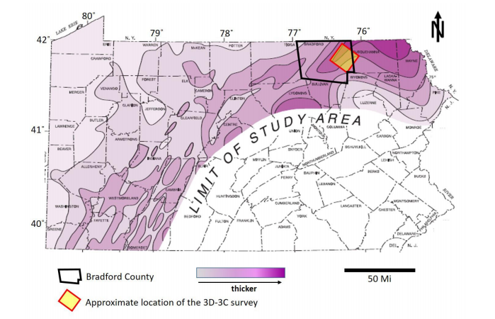
Figure 1: A map of Marcellus shale thickness in Pennsylvania overlain by the Bradford County and the approximate location of the survey outline. Figure reproduced from the masters thesis Pelayo, (2016).

3 Formalism

3.1 General notation

Throughout this document, we are going to indicate variables that are matrices in capitals ${\bf Y}$, and vectors using an the lowercase bold ${\bf y}$. Elements of a matrices and vectors will be labeled with subscript notation; e.g. $y_{ij}$ and $y_{i}$ for matrices and vectors respectively. The upper case super/subscript notation ${\bf Y}^{l}$ and ${\bf Y}_{l}$ indicates the rows and columns of the matrix respectively. The result being row and column vectors; the notation ${\bf Y}^{T}_{l}$ is meant to indicate that we are (in this case) taking the column of the matrix as a column vector and then transposing it to a row vector. As a special case, the symbol ${\bf\mathcal{I}}_{n}$, will represent the identity matrix, where the subscript indicates the rank of the matrix. Otherwise variables are considered to be scalars (or functions where appropriate). In terms of operators, $\rm sign({\bf B}^{l})$ is a vector whose elements are $\rm sign(b_{li})$, and the derivative $\frac{\delta}{\delta{\bf B}^{l}}$ should be interpreted as a gradient (a vector) whose elements are $\frac{\delta}{\delta b_{li}}$.

For the purpose of efficient computation, it is useful to use the Kronecker product and vectorization operators to account for the layout of the model. The Kronecker product ${\bf A}\otimes{\bf B}$, for a $(m\times n)$ matrix ${\bf A}$, and $(p\times q)$ matrix ${\bf B}$, for example, is:

$${\bf A}\otimes{\bf B}=\left[\begin{array}[]{cccc}a_{11}{\bf B}&.&.&a_{1n}{\bf B}\\ .&.&&\\ .&&.&\\ a_{m1}{\bf B}&&&a_{mn}{\bf B}\\ \end{array}\right]\ .$$

The vectorization operator acting on a matrix, simply stacks the columns of matrix into a vector:

$$\rm Vec({\bf A})=\left(\begin{array}[]{c}a_{11}\\ a_{21}\\ .\\ .\\ a_{nm}\\ \end{array}\right)\ .$$

A collection of useful identities associated with operations on matrices A, B, and C are:

$${\rm Inverse:}({\bf A}\otimes{\bf B})^{-1}=({\bf A}^{-1}\otimes{\bf B}^{-1})$$ (1)

$${\rm MatMult:}({\bf A}\otimes{\bf B})({\bf C}\otimes{\bf D})=({\bf AC}\otimes{\bf BD})$$ (2)

$${\rm MatVec:}({\bf C}^{T}\otimes{\bf A})\rm Vec({\bf B})=\rm Vec({\bf ABC})$$ (3)

$${\rm Vec:}\rm Vec({\bf AB})=({\bf B}^{T}\otimes{\bf\mathcal{I}}_{n})\rm Vec({\bf A})\ ,$$ (4)

for the final identity, $n$ is the number of rows of the matrix ${\bf A}$.

To denote statistical models, we use the notation $p({\bf A},{\bf B})$ to mean the joint probability of A and B, and $p({\bf A}|{\bf B})$ to denote the conditional probability. Bayes theorem would be expressed as:

$$p({\bf A},{\bf B}) = p({\bf A}|{\bf B})p({\bf B})\ .$$ (5)

3.2 Observational model

The input to the inversion is a seismic wavelet and a time migrated seismic data, organized by sectored angle and azimuth gathers or into offset vector tiles. We are going to structure the input seismic data as a matrix, with temporal and spatial (offset and azimuth) dimensions. We do not need to assume that the observations are regularly sampled by offset (or angle), only that the sampling in the offset and azimuthal domain is uniform.

Define a matrix ${\bf Y}$ of observations, the columns of which contain a trace of data at a particular coordinate in the offset/azimuth domain. The convolutional model of the earth expresses an observed seismic trace as a convolution of a wavelet with a sequence of reflectivities. The reflectivity is a function both of temporal and spatial coordinates of the trace, we will represent the reflectivity as a matrix ${\bf R}$, which has the same dimensions as ${\bf Y}$:

$${\bf Y}^{i}_{t} = (w*{\bf R}^{i})_{t}+{\bf\epsilon}_{t}\ ,$$ (6)

here $w$ represents the seismic wavelet and $\epsilon$ represents idiosyncratic noise (considered exogenous to the model), both are functions of time.

Continuing with the matrix notation, since the time sampling of the data is discrete, we can represent the convolution as a matrix-vector product. Suppose we have $T$ time samples and $N$ combinations of offset and azimuth in the gather, and that we use the same seismic wavelet for each coordinate. Then the observational model can be represented as a matrix vector product:

$$\rm Vec({\bf Y}) = (\mathcal{I}_{N}\otimes{\bf W})\rm Vec({\bf R})+\rm Vec({\bf E})\ ,$$ (7)

where ${\bf W}$ is a convolution matrix build from the seismic wavelet (which is circulant) dimension ($T\times T$). Matrices ${\bf Y}$, ${\bf R}$ and ${\bf E}$ contain the observations, reflectivity and noise respectively, each matrix has dimensions ($T\times N$).

The reflectivity at each point in time is very generally a function of offset and azimuth. We can represent any function on this domain as an expansion in some complete polynomial basis (or stacks),

$${\bf R} = {\bf B}{\bf A}^{T}\ ,$$ (8)

here ${\bf B}$ is a $(T\times r)$ matrix and ${\bf A}$ is a $(N\times r)$. The magnitude of the coefficients in the columns of the matrix ${\bf B}$ represent the weightings of the stacks. A constraint on the normalization of ${\bf A}$ become necessary for identifying the model; a convenient normalization is such that ${\bf A}$ is orthogonal. Re-factoring our observational model to a more convenient form:

$$\rm Vec({\bf Y}) = (\mathcal{I}_{N}\otimes{\bf W})\rm Vec({\bf B}{\bf A}^{T})+\rm Vec({\bf E})$$ (9)

$$= (\mathcal{I}_{N}\otimes{\bf W})({\bf A}\otimes\mathcal{I}_{T})\rm Vec({\bf B})+\rm Vec({\bf E})$$ (10)

$$= ({\bf A}\otimes{\bf W})\rm Vec({\bf B})+\rm Vec({\bf E})\ .$$ (11)

With the useful identities from the previous section, we can show that this is equivalent to a matrix equation of reflectivity convolved with a wavelet plus some idiosyncratic noise:

$${\bf Y} = {\bf W}{\bf B}{\bf A}^{T}+{\bf E}\ .$$ (12)

3.3 Statistical model and rank reduction

For the purpose of optimization, the form of Eq. 12 is not convenient because it is not linear in the set of parameters ${\bf B}$. To derive an equivalent linear problem, we have to first decided what the structure of the background noise is going to be. As an approximation, we will assume that the noise is normally distributed, and that the noise-model can be factorized in terms of the spatial (${\bf Q}$) and temporal (${\bf\Sigma}$) degrees of freedom independently,

$${\bf E}\sim{\bf\Sigma}\otimes{\bf Q},$$ (13)

In this case the likelihood function we would optimize for with respect to the matrix of coefficient ${\bf B}$ is matrix-variate normal (MVN) Gupta and Nagar, (2000),

$$\mathcal{L}({\bf Y}|{\bf B})=MVN({\bf Y};{\bf B}{\bf A},{\bf\Sigma},{\bf Q})\ .$$ (14)

To make the problem more tractable computationally, we will make the usual assumptions that the noise model can be represented as a scaled identity, ${\bf\Sigma}=\sigma^{2}\mathcal{I}_{T}$ and ${\bf Q}=\mathcal{I}_{N}$. This model for ${\bf\Sigma}$ means that we expect the noise is constant in time, and not correlated temporally. The model covariance ${\bf Q}$ means that we do not expect that the noise should be correlated between traces within a gather.

Now consider that spatially, reciprocity means that solution for an AVO analysis must only be non-zero for even basis functions. Therefore we know that the reflectivity matrix ${\bf R}$ must have a reduced rank. There are also physical reasons to suppose that the solution space should have a low dimension. For an application to unconventional resources, Glinsky et al., (2015) uses the floating grain model to decompose the AVO response in terms of its independent degrees of freedom. They find that only two- or three-independent pieces of information are likely resolvable for most applications. Practically this means that we can truncate the expansion at some order $r$ in our polynomial basis of choice. This truncation is equivalent to use setting the appropriate coefficient on the matrix ${\bf B}$ to zero. Following the approach of Chen et al.Chen and Huang, (2012), consider a complete set of orthonormal basis vectors packed into the matrix A,

$${\bf A}=[{\bf A}_{\bot},{\bf A}_{\parallel}]\ ,$$

where ${\bf A}_{\bot}$ is a (N$\times$r) matrix and ${\bf A}_{\parallel}$ is a (N$\times$(N-r)) matrix. To truncate the expansion, the coefficients of the matrix ${\bf A}_{\parallel}$ are set to zero. Taking advantage of the orthogonality of the basis functions, and our assumptions about the error model, the likelihood function becomes:

$$\mathcal{L}({\bf Y}|{\bf B}) = {\rm MVN}({\bf Y};{\bf W}[{\bf B}_{\bot},0][{\bf A}_{\bot},{\bf A}_{\parallel}]^{T},\sigma^{2}\mathcal{I}_{T},\mathcal{I}_{N})$$ (15)

$$= {\rm MVN}({\bf Y}{\bf A}_{\bot};{\bf W}{\bf B}_{\bot},\sigma^{2}\mathcal{I}_{T},\ I_{r})MVN({\bf Y}{\bf A}_{\parallel};0,\sigma^{2}\mathcal{I}_{T},\mathcal{I}_{N-r})\ .$$ (16)

The above is just statement of conditional probability of the matrix-variate normal. The second term in this equation is just a scalar. In the case where our input data is not regularly sampled, or where we what to regress on the more common ${1,\sin^{2},tan^{2}}$ basis, the approach is still applicable, but we need to use a QR-decomposition and solve an analogous preconditioned problem, this procedure is detailed in Appendix A. Dropping the ${\bot}$ subscripts from Eq. (15), we arrive at a simplified version of our likelihood function:

$$\mathcal{L}({\bf Y}|{\bf B}) \propto {\rm MVN}({\bf Y}{\bf A};{\bf W}{\bf B},\sigma^{2}\mathcal{I}_{T},I_{r}).$$ (17)

Optimizing this linear function is equivalent to solving Eq. 12, given the assumptions discussed above. An optimization algorithm for this equation subject to sparse penalties is derived in the Appendices.

3.4 Prior model - sparsity and smoothness

Temporally, our a priori expectation is that the earth response should be sparse and heavy tailed. This is consistent with an assumption of a layered earth, with relatively many bright reflectors (compared to Gaussian assumption). This is a common assumption made for post-stack sparse spike inversion, see Zhang and Castagna, (2011) as an example. Spatially; common models of amplitude variation by offset and azimuth, such as a Shuey and Ruger models are smooth. Distortion due to effects of NMO-stretch or attenuation should also be smooth. And so our prior model should reflect the sparse layered earth, and otherwise smooth amplitude variation by offset.

Post-stack, the reflectivity (as a function of offset) is projected onto constant stack weights to form a time-series. The L1-norm of this time-series reflects the prior assumption that the earth is sparse. Generalizing this to the pre- (or multi-) stack example, the negative log-prior (up to a constant in ${\bf B}$) is:

$$p({\bf B}) = \lambda\|\rm Vec({\bf B})\|_{1}\ ,$$ (18)

where $\lambda$ is the rate parameter of the Laplace distribution. This kind of prior assumption induces a sparse solutionSassen and Glinsky, (2013) and Sassen and Lasscock, (2015), however, except in the special case of a post-stack inversion, we cannot directly interpret this in terms of the sparse layered earth. Rather, this prior makes a statement regarding the overall complexity of the solution.

Instead we introduce a new prior model for sparse inversion of seismic data basedChen and Huang, (2012),

$$p({\bf B}) = \sum_{t=1}^{T}\lambda_{t}\|{\bf B}^{t}\|_{2}\ ,$$ (19)

where $\lambda_{t}$ is now a collection of rate parameters, on for each point in time, and $\|\cdot\|_{2}$ is the Euclidean norm. Following the statistical literatureFriedman et al., (2010), we can view the parameterization of the AVO(z) response at each time as a group. This prior induces sparsity in terms of the groups, the inversion will then be sparse in terms of which groups are active (in-active groups are thresholded uniformly to zero). Where, in our application, an active group at a point in time represents the location of a reflector. Otherwise, we are not enforcing a sparse penalty on the complexity of the AVO(z) response within each group. Therefore, this prior model represents the belief that the AVO(z) response is smooth, but the earth is sparse and layered. Note, there is a crucial difference in behavior between the canonical L1 and sparse grouped priors for the specific application to an azimuthal inversion. Consider that the change in reflectivity is a function of azimuth measured relative some axis of symmetry that is a priori unknown. The regression problem must be applied to a set of azimuthally varying functions, where azimuth is defined in some arbitrary orientation, with respect to true or grid North for example. Since this orientation is arbitrary, the invariances of the prior model subject to a rotation of the coordinate system is important. The analysis of ChenChen and Huang, (2012) shows that the location of the reflectors in time, generated by the sparse grouped prior model Eq. 19 are guaranteed to be invariant under a rotation of the coordinate system. However, the usual L1-prior applied to the azimuthal inversion is not.

Whilst both the noise model and importance of the layer based prior may be functions of time, calibration of this expansive parameter space is beyond the scope of this paper. For the remainder of this article we will deal with the special case where both are constant in time. Since our analysis will center around a limited time window around the Marcellus shale, this is a reasonable simplification. Combining our prior model with the likelihood function Eq. (17), the negative log-posterior probability (up to an additive constant in ${\bf B}$) we seek to minimize is the matrix-variate function:

$${\rm log}(p({\bf B}|{\bf Y})) = \frac{1}{2\sigma^{2}}\|{\bf Y}{\bf A}^{T}-{\bf W}{\bf B}\|^{2}_{2}+\lambda\|\rm Vec({\bf B})\|_{1}+\ \lambda_{g}\sum_{t=1}^{T}\|{\bf B}^{t}\|_{2}\ .$$ (20)

The method for optimizing this model is detailed in Appendix B. Note that we are detailing a particular choice for the grouped constraint, where we group by row. However, the optimization applies equally where the groups span for multiple rows of ${\bf B}$.

4 Method

The Appendices detail a very general model for inverting for the azimuthally varying AVO response. The inputs to the model are a wavelet, extracted at a well using a 25-degree stack and a HTI corrected set of time migrated offset vector tile (OVT) gathers.

The sparse inversion is performed on a time interval between the Tully and Onondaga limestone. We linearly interpolate a set of hand picked horizons across the survey. The inverted attributes are a sequence of sparse spikes, which do not necessarily lie exactly along the interpolated horizon. We therefore perform a search for the nearest peak (or trough depending on the horizon) within 6ms of the horizon picked at each inline and associate that with the spike. Since the spikes themselves have a finite bandwidth, a secant area methodGlinsky et al., (2016) is used to integrate the spikes.

The region that is of particular commercial interest is the so called Hot Marcellus, which is a thin layer of high total organic content (TOC) shale which sits atop the Onondaga limestone. We will provide interpretation of the inversion for this horizon. To classify each point on the horizon using the estimated attributes, we apply a unsupervised clustering Expectation Maximization (EM) algorithm. The EM-algorithm takes as input the expected number of clusters, it then fits a multivariate Gaussian density to describe the distribution of points within each cluster. The EM-algorithm is similar to the K-means classifier commonly used in seismic attribute analysis, except that it clusters are hyper-ellipsoidal rather than strictly hyper-spherical. Given the elliptical relationships commonly seen cross-plotting rock-physics relationships, the EM-classifier is more general and more appropriate for this kind of attribute analysis.

We do not know the number of clusters a priori, our method for calibrating this is to sequentially add more clusters to the model, stopping once we found a parsimonious description of the horizon. Assuming the elastic properties of the shale and limestone are fairly stationary spatially, we expect that there should be at least two classes of material, which we may expect to interpret as fractured or non-fractured. Since we do not have sufficient well measurements to allow us to characterize the clusters directly, we need to appeal to a particular model for the AVO response for interpretation. Following Tylasning Tylasning and Cooke, (2016), we will interpret the reflectivity in terms of Ruger’s two-term modelRuger and Tsvankin, (1997). Assuming Ruger’s model, we derive an estimate of the anisotropic gradient, and fracture orientation, up to a $90^{\circ}$ ambiguity. In a recent study by Sclanser et al., (2016), the EM-algorithm was applied to well-log data for the purpose of classifying litho-facies. This study identifies four classes of shale, and a carbonate in our area of interest. The results of this analysis are used to provide a comparison with the two estimates of isotropic gradient predicted by the Ruger model. The solution that is consistent with the regional data resolves the $90^{\circ}$ ambiguity. Note, the inversion will be performed with sufficient degrees of freedom to allow us to interpret a higher order model, however we will leave that as future work.

4.1 Interpretation

Consider an inversion of data which at each point in time has spatial degrees of freedom of offset and azimuth. For example where the input data is a set of offset vector tiles (OVT). The domain of the problem is an azimuths ($\phi$) between 0-180-degrees (reciprocity makes the backward angles redundant) and range of offsets ($x$) normalized to the interval $[0,1]$.

We normalize measured offsets within the gather to on the interval [0,1], azimuth is measured on the interval [0,$\pi$]. Reciprocity demands that the reflectivity is symmetric under reflections, so we can imagine that the domain of the problem by offset is [-1,1], but that the solution should be symmetric, which we enforce. The basis of spherical harmonic function $Y_{lm}(x,\phi)$ is complete on this domain. Therefore very generally, any smooth function of the reflectivity can be represented by this expansion:

$$r(x,\phi) = \sum_{lm}a_{lm}Y_{lm}(x,\phi)\ .$$ (21)

Here the coefficients $a_{lm}$ would be the most general set of attributes, however, for computational efficiency we appeal to physical modeling to reduce the dimension of this parameter space.

For the sake of computational convenience, we would look to reduce the dimension of the parameter space by supposing that we can truncate the polynomial expansion to some order. Having decided where to truncate the expansion, we will then require a method of interpretation given a physical model. For our demonstration to the Marcellus shale, we will analyze data with incident angles out to $35^{\circ}$. A suitable physical model of the reflectivity on this domain is according to Ruger and Tsvankin, (1997), in terms of the angle of incidence $\theta(x)$ and azimuth $\phi$:

$$r(x,\phi) = I+({\rm B}^{iso}+{\rm B}^{ani}\cos^{2}(\phi-\phi_{s}))\sin^{2}(\theta(x))$$ (22)

$$= I+({\rm B}^{iso}+\frac{B^{ani}}{2})\sin^{2}(\theta(x))+\ \frac{B^{ani}}{2}\cos(2\phi_{s})\cos(2\phi)\sin^{2}(\theta(x))+$$ (24)

$$\hskip 85.35826pt\frac{B^{ani}}{2}\sin(2\phi_{s})\sin(2\phi)\sin^{2}(\theta(x))\ .$$

The $\cos(2\phi),\ \sin(2\phi)$ dependence in the azimuth is orthogonal to the harmonic functions with $l>2$. By reciprocity, only even coefficients of $|m|$ are non-zero. Now consider the angular dependence by offset. The simple angle-to-offset transformCastagna and Backus, (1993):

$$\sin^{2}(\theta(x)) = \bigg{(}\frac{v_{\rm int}}{v_{\rm rms}}\bigg{)}^{2}\frac{x^{2}}{x^{2}+(v_{\rm rms}t_{0})^{2}}\ ,$$ (25)

(within approximately $30^{\circ}$), converges very rapidly in the basis of Legendre polynomials. The weights for the expansion:

$$\sin^{2}(\theta(x)) = \sum_{i}w_{i}P_{i}(x),$$ (26)

of even $x$, are shown in Fig. 2 for typical values of rms- and interval velocity.

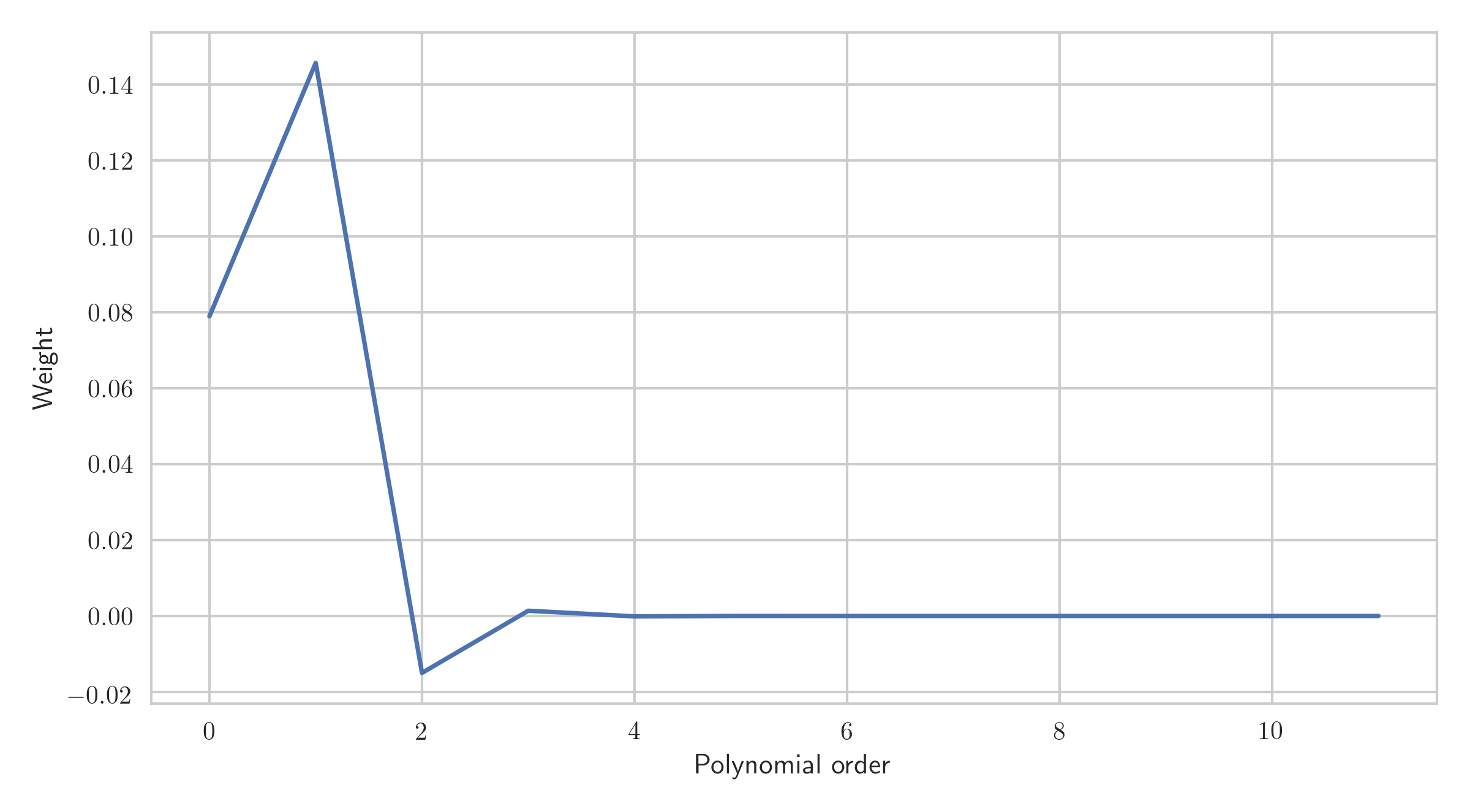
Figure 2: The weights for an expansion of the $\sin^{2}(\theta(x))$, based on the angle to offset transform parameterized for typical interval ($v_{\rm int}$), and rms ($v_{\rm rms}$) velocities at the base of the Marcellus shale.

With these constraints, it is computationally convenient to do our regression on a re-summed expansion of the spherical harmonics in terms of the Legendre polynomials:

$$r(x,\phi) = \sum_{i=0}\bigg{(}a_{i0}P_{i}(x)+a_{i1}P_{i}(x)\sin(2\phi)+\ a_{i2}P_{i}(x)\cos(2\phi)\bigg{)}\ .$$ (27)

Given the analysis shown in Fig. 2, we will truncate the expansion of the reflectivity in the basis of Legendre polynomials at 6-th order (inclusive), using only the even polynomials. The attributes $a_{ij}$ are a set of coefficients associated with each basis function, these basis functions are orthogonal.

Combining Eqs. (22), (26) and (27) we have a table of relationships:

$$a_{00} = I+\bigg{(}{\rm B}^{iso}+\frac{B^{ani}}{2}\bigg{)}w_{0}$$ (28)

$$a_{i0} = ({\rm B}^{iso}+\frac{B^{ani}}{2})w_{i}$$ (29)

$$a_{i1} = \frac{B^{ani}}{2}\sin(2\phi_{s})w_{i}$$ (30)

$$a_{i2} = \frac{B^{ani}}{2}\cos(2\phi_{s})w_{i}\ ,$$ (31)

the weights $w_{i}$ can be estimated by ray tracing, or using the angle-to-offset transform. From the relationships Eq. (28) we can immediately solve for azimuthal variables:

$$\frac{|B^{ani}|}{2}|w_{i}| = \sqrt{a_{i1}^{2}+a_{i2}^{2}}$$ (32)

$$2\phi_{s} = \arctan{\bigg{(}\frac{a_{i1}}{a_{i2}}\bigg{)}}\ ,$$ (33)

with the solution for isotropic intercept as:

$$I = a_{00}-a_{i0}\frac{w_{i}}{w_{0}}$$ (34)

The solution for the isotropic gradient is somewhat ambiguous. From Eq. (22), we solve for the magnitude of the anisotropic gradient, but can only estimate the orientation of the axis of symmetry up to an overall phase of $90^{\circ}$. The isotropic gradient cannot be unambiguously estimated without first knowing the sign of the anisotropic gradient:

$$B_{\rm iso}w_{i} = a_{i0}\pm\frac{|B^{ani}|}{2}w_{i}$$ (35)

$${\rm or\ }$$ (36)

$$B_{\rm iso}w_{i} = a_{i0}\pm\bigg{(}a_{j1}\sin(2\phi_{s})+a_{j2}\cos(2\phi_{s})\bigg{)}\frac{w_{i}}{w_{j}}\ ,$$ (37)

While both of these equations are valid, in the presence of noise, the distribution of $|B^{ani}|$ becomes skewed, and heavy tailed. We expect that propagating this uncertainty will lead to a skewed estimate of $B_{\rm iso}$. Finally, assuming stationarity in $\phi_{s}$, we choose the solution for the isotropic gradient that is consistent with the regional analysis of Sclanser et al., (2016).

These relationships are valid for all $w_{i}\neq 0$, solutions for $I$, $B_{iso}$, $B_{ani}$ and $\phi_{s}$ are determined by averaging the appropriate normalized coefficients at over every order in the expansion. To translate this result to our master formula Eq. (20), pack the basis vectors:
$\{P_{0}(x_{i}),\ P_{0}(x_{i})\sin(2\phi_{i}),\ P_{0}(x_{i})\cos(2\phi_{i}),\ ...\}$ into the columns of matrix $A$ for each trace $i$ of the gather. The rows of the solution $B$ contains the coefficients $a_{lm}$ at each point in time. The coefficients $a_{lm}$ describe the reflectivity surface at a particular time, a clustering algorithm is applied in this space for a particular horizon.

5 Results

5.1 Synthetic Example

We will first demonstrate the algorithm on a simple synthetic data forward modeled using the Geokinetics’ SynAVO package, with modifications to simulate the azimuthal variation in reflectivity. The SynAVO forward model used a 40Hz Ricker wavelet, with effects of NMO-stretch included in the model. Rock-properties for the reflectors were take from the example Table 1 of Ruger and Tsvankin, (1997), with an axis-of-symmetry at $30^{\circ}$. The sequence in each case is an anisotropic material layered between two isotropic materials. The model simulates fluid filled cracks in a thin layer 75ft in thick, surrounded by an isotropic material. We simulate an OVT gather by forward modeling the seismic response using a (10x5) grid of tiles, each separated by 350ft in each spatial direction.

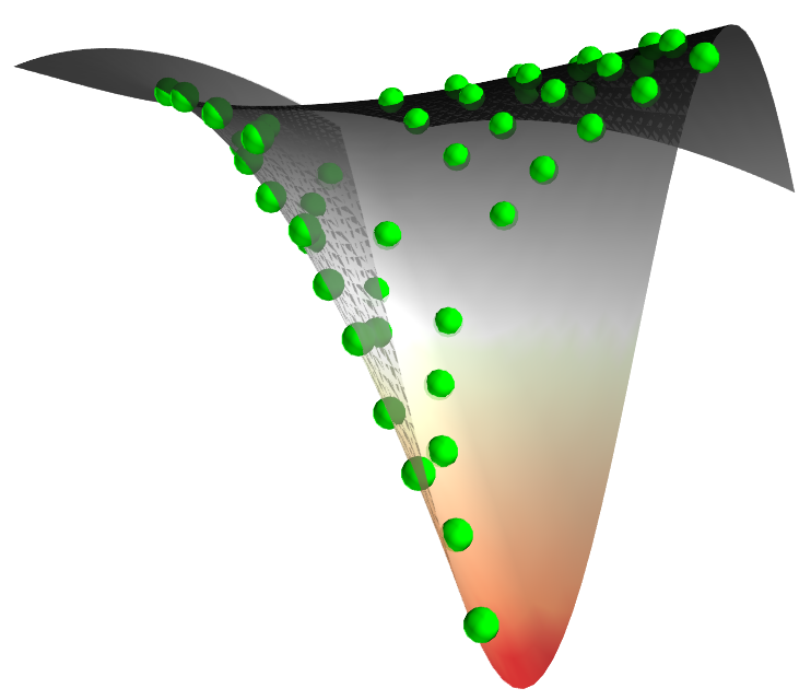
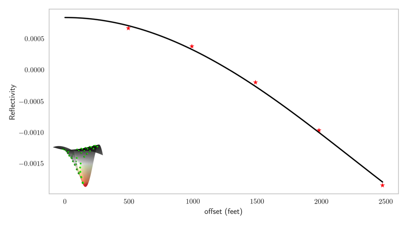
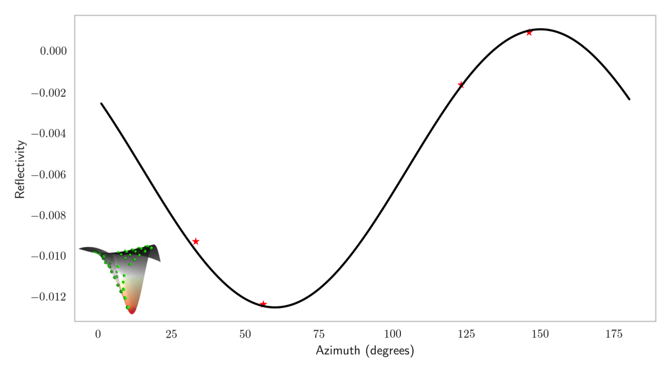
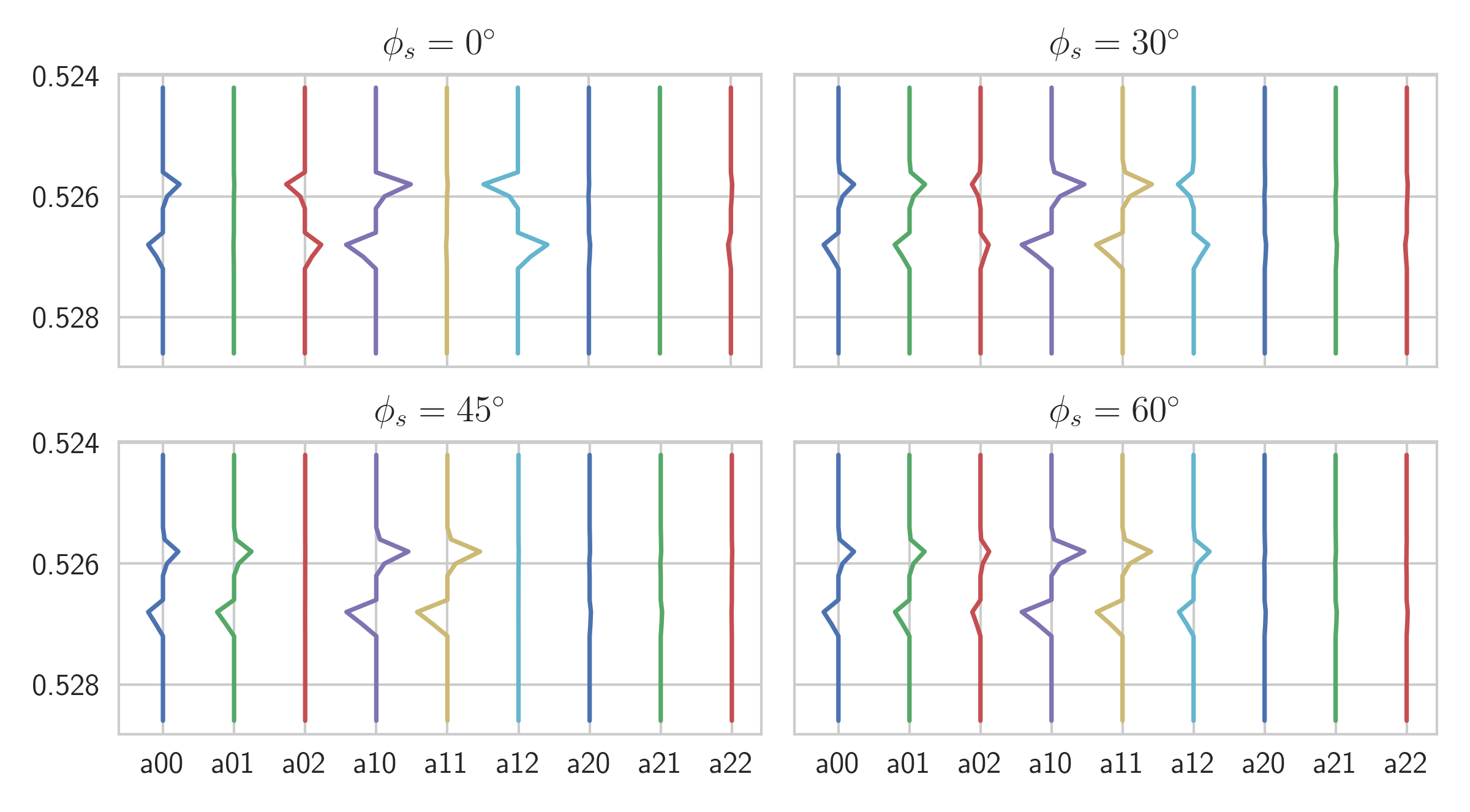
Figure 3: (top left) Demonstrates the reflectivity surface inverted from the synthetic example at the base of the layer simulating fluid filled cracks. The vertical axis is amplitude, the horizontal axes are spatial. (green points) The amplitude of the seismic simulated by SynAVO at each offset and azimuth. (top right) At a fixed azimuth of $134^{\circ}$, (black line) the reconstructed seismic from the inversion as a function of offset. (red star) The synthetic data. (bottom left) Similarly, the reconstructed seismic and synthetic data at fixed offset of 1250 feet. (bottom right) The spikes at each order of the expansion for the synthetic example, (clockwise) the axis-of-symmetry is rotated from $0^{\circ}$ to $30^{\circ}$, $60^{\circ}$ and $45^{\circ}$ respectively.

The (green) points in Fig. 3 (top left) show the amplitude of the synthetic gather as a function of offset and azimuth, at the base of the simulated thin layer of wet cracks. The optimization solves for attributes $a_{ij}$ using the methods discussed above, where we have applied the grouped sparse constraint only. Combining the inverted attributes, with the polynomial basis gives a a formula for the reflectivity surface Eq. (27) (a function of offset and azimuth). Convolving the reflectivity with the wavelet provides a reconstruction of the seismic as a function of offset and azimuth. This surface is overlayed on the image (top left). The dimensions of this image are amplitude (vertical axis) and spatial (horizontal axes). To further demonstrate the geometry of the problem, (top right) and (bottom left) we show cut planes through the surface at a particular offset and azimuth respectively. Here the (black line) represented the reconstruction and (red star) shows the synthetic data. The reconstruction is not exact because of the effect of NMO-stretch, and because the optimization faces a trade-off between minimizing both the residual variance and the complexity of the solution. Where minimizing both absolutely is mutually exclusive.

The optimization framework we derive is very general, for a specific application to real seismic data, we analyze the reflectivity according to Ruger’s model using the formula derived above. In Fig. 3 (bottom right) we show the inverted attributes which appear as a sequence of sparse spikes. Here we resolve the top and base of the reflector in the synthetic example. The spikes have a finite bandwidth because the optimization cannot identify the location of the reflector with resolution that exceeds the Nyquist criterion. The amplitude of the reflectivity at a horizon is found my integrating the spikes, a secant method, such as Glinsky et al., (2016) would be appropriate. The first three attributes in each image are associated with the $P_{0}(x)$, polynomial, the next three are associated with the $P_{1}(x)$ polynomial, an so on. Our expectation for the relative amplitude between these groups is shown in Fig. 2, with the largest power associated with the $P_{1}(x)$ polynomial and a very rapid convergence of the $\sin^{2}(\theta(x))$ dependence in the basis of Legendre polynomials. From Eq. (28), the amplitude of the $a_{00},\ a_{10},\ a_{20}$ attributes come from a mixture of isotropic and anisotropic gradient, where the amplitude of the $a_{i1},\ a_{i2}$ attributes originates solely from the presence of the anisotropic gradient. Recall that $a_{i1},\ a_{i2}$ are proportional to the sine and cosine of twice the axis-of-symmetry ($\phi_{s}$, relative to grid north). As the axis-of-symmetry rotates in this example, we see the spectral content moving from the $a_{i2}$ attributes at $\phi_{s}=0^{\circ}$, to the $a_{i1}$ attributes at $\phi_{s}=45^{\circ}$. Once the axis-of-symmetry reaches $\phi_{s}=90^{\circ}$, the spectral content has rotated back to the $a_{i2}$ attributes, which is indistinguishable from the $\phi_{s}=0^{\circ}$. This represents the so-called $90^{\circ}$ ambiguity in the two-term version of Ruger’s model.

5.2 Application to the Marcellus - Calibration

In this section we will apply the sparse azimuthal inversion to field data. The geological setting and aspects of the aquisition were discussed previously.

To parameterize the model Eq. (20), we need an estimate of the seismic noise level and a value for the sparse constraint, where we will use the same value for the group constraint ($\lambda_{g}$) for all time. Practically it is the product of the prior rate parameter $\lambda_{g}$ and the noise-level $\sigma^{2}$ that will effect the result of the inversion, as such we only need a approximate estimate of the noise level in order to have a good initial guess of what the optimal value for $\lambda_{g}$ might be. The median variance of a seismic trace computed from all gathers within the dataset is used to set the background noise level. A better estimate of the seismic noise level could also be estimated jointly with the wavelet extraction using a Bayesian methodology such as Gunning and Glinsky, (2006).

Given this estimate of the noise level, we explore values of $\lambda_{g}$ for a given inline, as shown in Fig. 4 (top left). The goal is to find the least complex model that can explain the variability in the data. In our example there are two very prominent reflectors, which are the Tully and Onondaga limestones. To calibrate $\lambda_{g}$, we start with a value that will resolve these features, and little else. Then allow the complexity of the model to increase by reducing the value of $\lambda_{g}$. The exponential of the relative Akaike information criteria (AIC) for a series of values of $\lambda_{g}$ is shown in Fig. 4. This curve reflects a trade-off between the ability of the model to explain the variance in the data, and the complexity of the model. We choose the knee-point of this curve as the ideal trade-off between these competing goals.

As a quality control, we will analyze a particular gather from the dataset. In Fig. 4 (top right) we show a the gather as a function of time, where the traces are sorted by offset and azimuth, note that the OVT data is not regularly sampled in this domain. The inversion is then done with $\lambda_{g}=0.20$, the resulting spikes are then re-convolved with the wavelet to give a reconstructed gather, this is shown (bottom right). The residual difference between the input and reconstructed gathers are shown (bottom left). From the point of view of the model, the residual is random, band-limited noise.

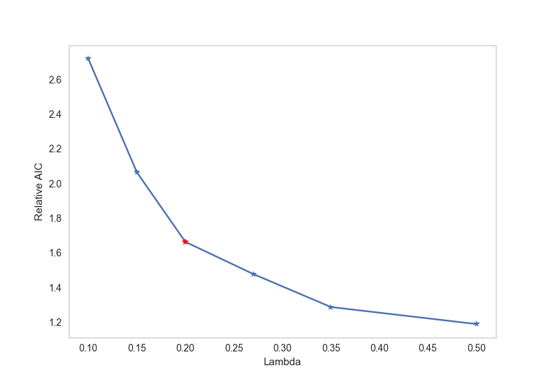
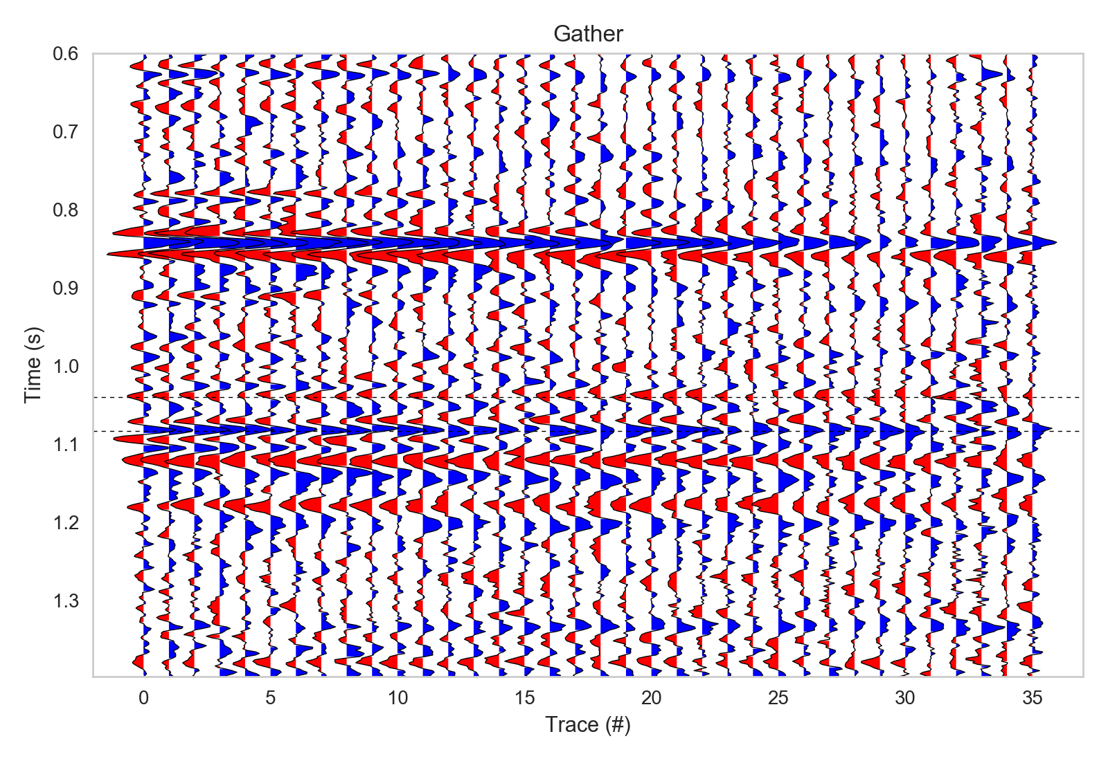
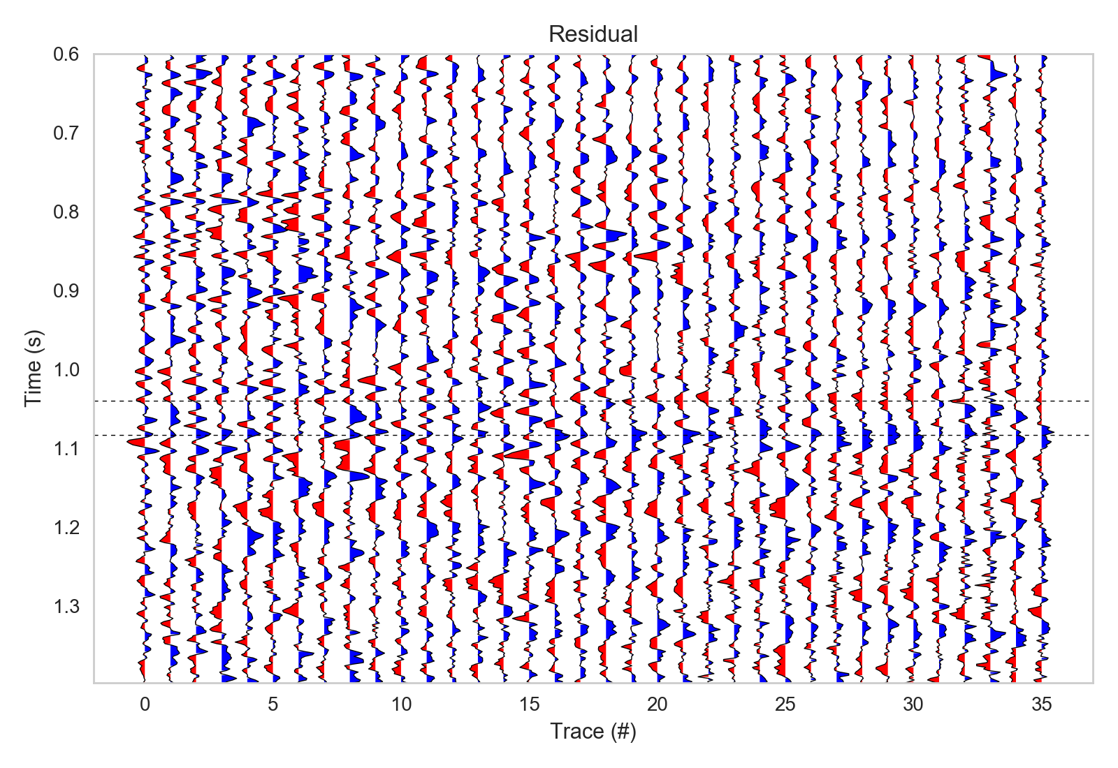
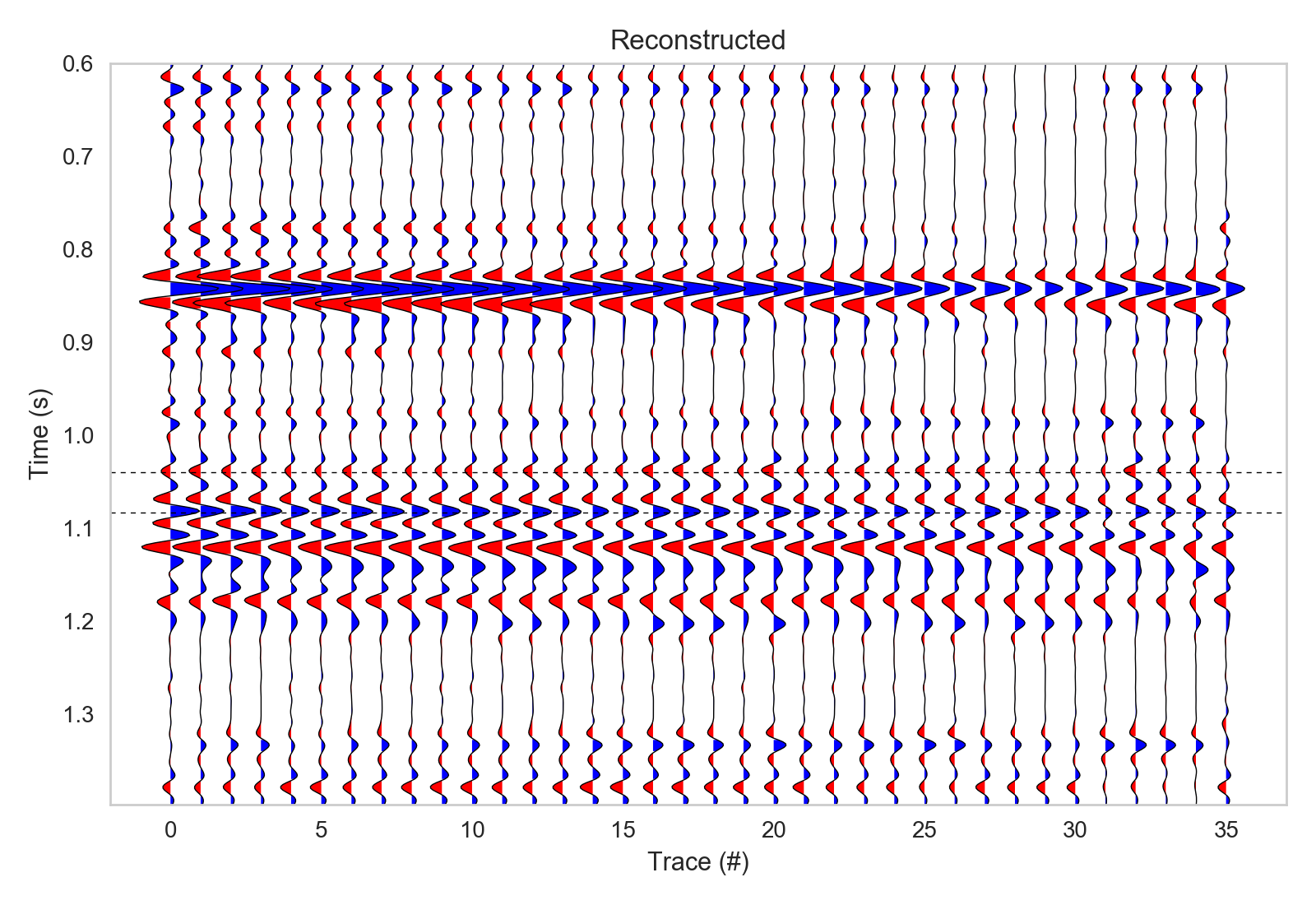
Figure 4: (top left) The relative Akaike information criteria for various values of the $\lambda_{g}$. (red star) The value of $\lambda_{g}$ used for the analysis throughout. (top right) An example OVT gather with traces ordered by offset and azimuth. (bottom right) The OVT gather reconstructed by convolving the extracted wavelet with the estimated reflectivity. (bottom left) The difference between the original and reconstructed gather.

The inverted reflectivity form this analysis are shown in Fig. 5 (left). For comparison, we plot the inverted spikes for a model where we only use the global sparse constraint (calibrated to produce an equivalent residual variance). The two models produce a very similar picture of which reflectors are important for describing variability in the data, however the grouped constraint does not provide the same penalty on the model complexity by offset and azimuth for a given reflector.

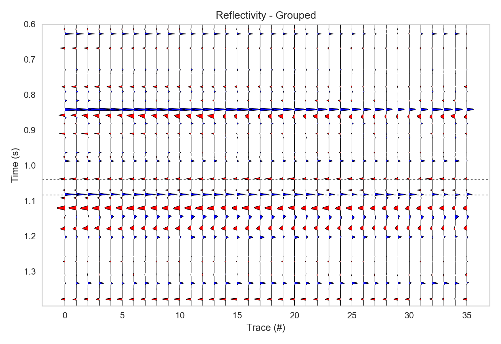
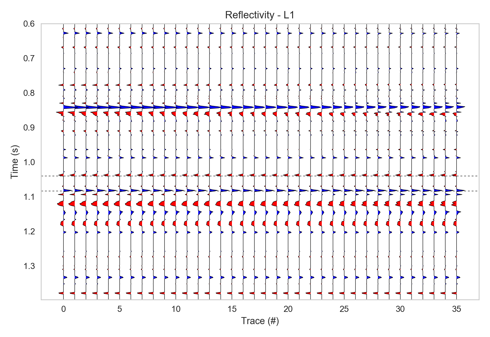
Figure 5: (left) Reflectivity inverted from the gather shown in Fig. 4 using only the grouped constraint. (right) A hypothetical equivalent reflectivity inverted using a standard L1-constraint.

Finally, the AIC provides a very general method for calibrating the model, however there is some largess for the user to vary the model complexity given an understanding of geology. In Fig. 6, we show a crude inversion of relative acoustic impedance derived from the reflectivity Fig. 5 (left). Here we take the cumulative sum of the inverted reflectivity at the nearest offset. We then apply a high-pass filter with a corner frequency of 6Hz. The location of the example gather is shown with the vertical dashed line, the picked horizons for the top and base of the Marcellus are shown as (solid red) and (dashed red) lines respectively. Interpretation of well-log data suggests the presence of the so-called “Hot Marcellus” in this area. The Hot Marcellus is a thin layer just above the Onondaga limestone that is characterized by relatively high total organic content compared to upper Marcellus. This is indicated in the crude inversion by a dip in acoustic impedance, which we see evidence for in Fig. 5 (above the red dashed line). We find that the statistically calibrated model $\lambda_{g}=0.20$ is sufficiently complicated to reveal this feature.

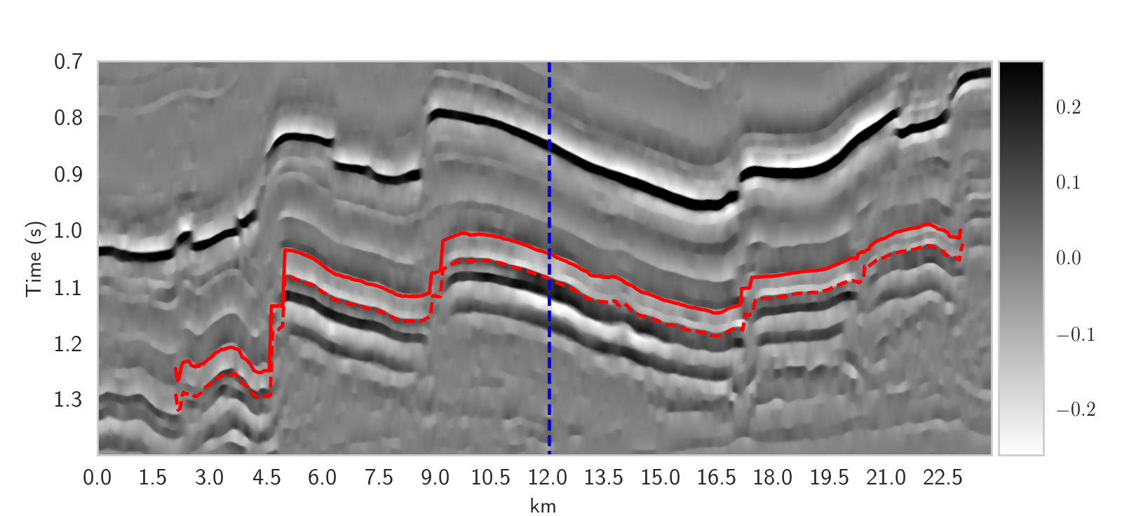
Figure 6: (top left) A crude inversion for relative acoustic impedance on an inline. (dashed blue) Indicates the location of the gather used in calibration. (solid red) Line shows the horizon at the top of the Marcellus shale. (dashed line) Line shows the horizon at the top of the Onondaga limestone (base of the Marcellus)

5.3 Application to the Marcellus - Unsupervised learning

Repeating the inversion for a set of gathers within a 3D seismic survey, a hand picked horizon at the base of the Marcellus is used to extract the coefficients of the expansion (Eq. (27)) for this reflector. These coefficients represent a concise description of the reflectivity surface at each point on the horizon. We can then apply an unsupervised learning algorithm determine if these coefficients are clustered in the parameter space. The EM-classifier we use to do this requires us to specify the number of clusters present. To determine this number we successively increase this number from one, until the addition of a cluster does not appear to group the data spatially. Using this method we arrived at three clusters, one of which groups the data around faults where our picked horizon is less reliable. We find that the performance of the classifier can be improved by first normalizing the coefficients using the relevant weights $w_{i}$ (computed from the angle-to-offset transform) to adjust for differences in the angle of incidence across the horizon.

Having identified spatial structure in the inverted coefficients, we now have a problem of interpretation, for this we need to appeal to a physical model. The coefficients of Ruger’s model are determined using the method described above. The ambiguity in the sign is resolved by ensuring that the isotropic gradient is consistent with regional data derived from Sclanser et al., (2016). The model parameters for base of Marcellus are shown in Fig. 7. The application of the clustering algorithm is shown in Fig. 8, overlayed onto the magnitude of the anisotropic gradient (that we may estimate unambiguously).

In Fig. 9 (right top and bottom) we show a histograms of the phase and magnitude of the anisotropic gradient for each class, and the distribution for the top decile of anisotropic gradient respectively. We see that the tail of the distribution is dominated by a single class. Interpreting one class as capturing areas around faults and at the periphery of the survey, the other two are characterized evidence of fracturing. Finally in Fig. 9 (left top and bottom) we show the distribution of $\phi_{s}$ (up to $90^{\circ}$), compared to the direction of the fast HTI velocity (overlaid), this data is taken from the HTI time migration. We see good agreement between the two analyses.

Finally, in Fig. 10 we cross-plot the distribution of intercept and gradient terms for each class. The (black star) marks forward modeled values of intercept and gradient derived from the P-wave velocity and density values for the gray-, dark gray-, black- and calcareous-shales interfacing with a carbonate. The values used were taken from Sclanser et al., (2016) for the Northern Pennsylvania region (Zone A). This data was derived from multiple well-logs in the zone of interest. Since S-wave velocity is not supplied in Sclanser et al., (2016), we used the Castagna-Greenberg relations to model this for the shales and carbonates respectively Mavko et al., (2009). As expected, that the range of isotropic gradient is greater for the class we associate with the fracturing. One likely explanation for this is that the variance in the estimate of the isotropic gradient is additive with the variance in the estimate of the anisotropic gradient, contaminating the estimate of isotropic gradient with additional noise. For the unfractured class, the center of the distribution was consistent with the intercept and gradient derived from the high TOC dark gray- and black-shales, layered on top of the carbonate. This is consistent with our observation of the “Hot Marcellus”, a high TOC shale, that we saw evidence for in Fig. 4.

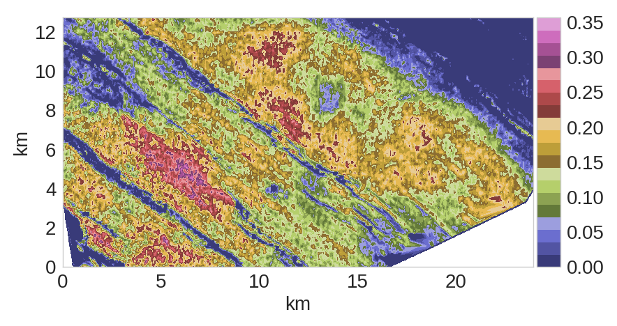
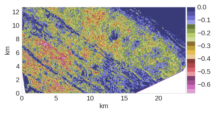
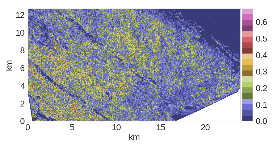
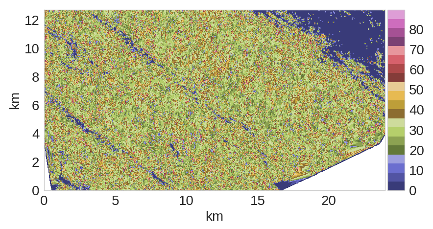
Figure 7: Horizons at the base of the Marcellus showing (top left) the intercept, (top right) the isotropic gradient, (bottom left) the anisotropic gradient and (bottom right) the orientation of the axis of symmetry of the fractures.

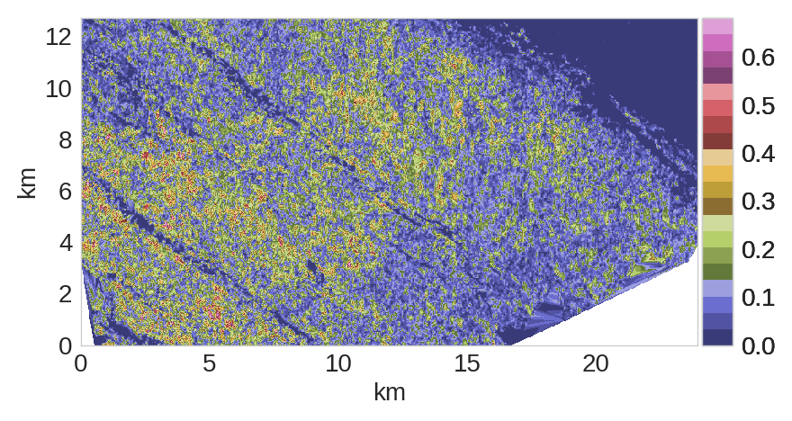
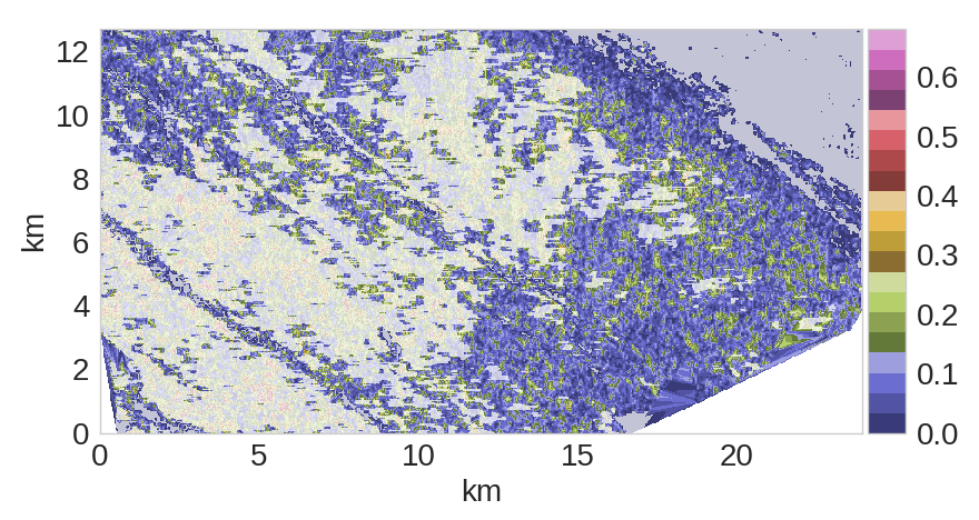
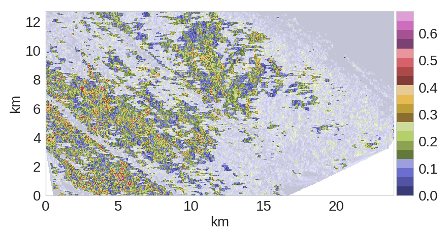
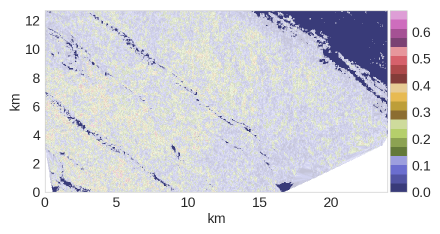
Figure 8: For the horizon at the base of the Marcellus, showing (top left) The magnitude of the anisotropic gradient. (otherwise) The magnitude of the anisotropic gradient for each cluster identified in the parameter space of the coefficients $a_{ij}$ defined in Eq. (27).

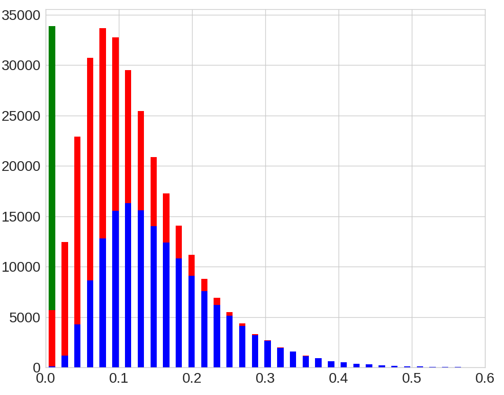
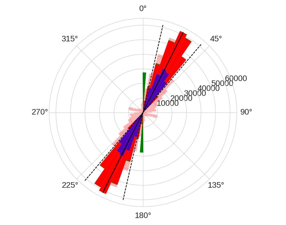
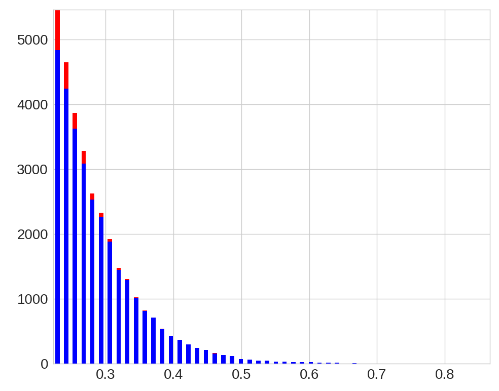
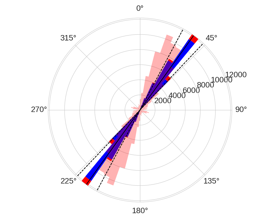
Figure 9: For the horizon at the base of the Marcellus. (top left) The distribution of the magnitude of anisotropic gradient. (bottom left) The same distribution magnifying the top decile sorted by the magnitude of anisotropic gradient. (top right) The distribution of estimates of the axis-of-symmetry, overlayed (light red) the distribution of the axis-of-symmetry estimated using the HTI-correction. (bottom right) The distribution of the axis-of-symmetry for the top decile of points sorted by the magnitude of anisotropic gradient.

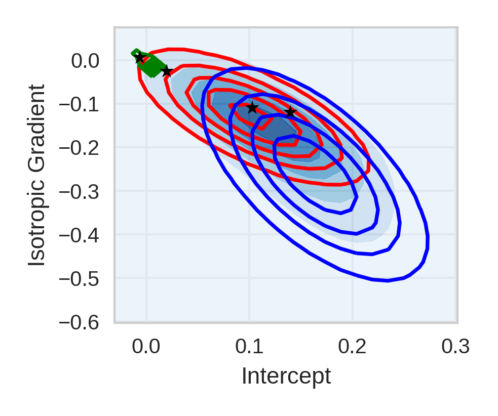
Figure 10: The distribution of the intercept and isotropic gradient values for each class. (blue) The distribution of intercept and isotropic gradient for the fractured class, (red) similarly for the unfractured class. The (green) class absorbs the zero and outlier data. (black star) Marks the modeling intercept and isotropic gradient using elastic properties derived for the gray shale, dark gray shale, black shale and calcareous from Sclanser et al., (2016). The interface is assumed to be the carbonate, with properties derived from the same paper.

6 Conclusions

In this paper we derived a method for estimating independent attributes describing reflectivity by offset and azimuth. The inversion was subject to very general prior assumptions about sparsity of the layered earth and smoothness of the reflectivity surface. Otherwise we did not presume that any particular physical model should apply, but let the data drive the inversion. Given an inverted set of independent attributes we then applied a clustering algorithm to classify the parameter space for a horizon at the base of the Marcellus shale. To improve the robustness of the statistical analysis, our method was derived to take common-offset or offset vector tiles as direct input, without the need for interpolation or fold-compensation that is required for processing sectored azimuthal gathers. We argue that the assumptions of sparsity and smoothness are guaranteed to be AVO compliant, and so reduce potential sources of bias from the processing.

We then presented an analysis of the Marcellus shale as an example application of our workflow. The target of the analysis was a horizon at the base of the Marcellus shale. We estimated AVO attributes encoding our knowledge of the reflectivity without reference to a specific physical model. We then applied an unsupervised learning algorithm (EM algorithm) in this space of attributes. Interpreting the result in the context of Ruger’s model, we computed the magnitude of the anisotropic gradient and compared the populations of the learned classes. Sorting the observed magnitude of anisotropic gradient, we saw that the top decile of values could be attributed to one class in particular. We also compared the estimated axis-of-symmetry $\phi_{s}$ using Ruger’s model to the fast velocity direction estimated from the HTI-migration. We can only resolve the orientation of $\phi_{s}$ to within $90^{\circ}$, however we found that it was consistent with the HTI-velocity analysis.

We then compared the estimates of the intercept and isotropic gradient to values forward modeled from well-logs in the region. Regional models where derived for four types of shale layered on top of a limestone. Models of the two high TOC dark gray- and black-shales lay at the center of cross-plots of inverted intercept and isotropic gradient for the Marcellus shale dataset we analyzed. The distribution of isotropic gradient was broader for the class associated with the large values of anisotropy. We note that since estimates of intercept, isotropic- and anisotropic-gradients are not made independently, uncertainty in the estimate of anisotropic gradient propagates through to the estimates of intercept and isotropic gradient.

Treatment of non-orthogonal bases functions

The master equation Eq. 17 assumes orthogonality of the basis vectors packed into the columns of the matrix ${\bf A}$. Irregular sampling of the data spatially, or a preference for a solution in a non-orthogonal basis breaks this constraint. In this case we need instead solve a preconditioned version of the problem.

The QR decomposition of the matrix ${\bf A}$ can be written,

$${\bf A}=\left[\begin{array}[]{cc}{\bf Q}_{11}&{\bf Q}_{22}\\ \end{array}\right]\left[\begin{array}[]{cc}{\bf R}_{11}&{\bf R}_{12}\\ {\bf 0}&{\bf R}_{22}\end{array}\right]$$

where ${\bf Q}_{11}$ is (N$\times$r) and ${\bf R}_{11}$ is (r$\times$r). Provided the matrix of basis functions ${\bf A}_{\bot}$ is full rank, the above expression is true if we define ${\bf Q}_{11}$ and ${\bf R}_{11}$ according to its QR factorization:

$${\bf A}_{\bot}={\bf Q}_{11}\left[\begin{array}[]{c}{\bf R}_{11}\\ {\bf 0}\end{array}\right]$$

The residual from Eq. (17) can be expressed as,

$${\bf Y}-{\bf W}\left[\begin{array}[]{cc}{\bf B}_{\bot}&{\bf 0}\\ \end{array}\right]\left[\begin{array}[]{cc}{\bf R}^{T}_{11}&{\bf 0}\\ {\bf R}^{T}_{12}&{\bf R}^{T}_{22}\end{array}\right]\left[\begin{array}[]{c}{\bf Q}^{T}_{11}\\ {\bf Q}^{T}_{22}\end{array}\right]$$

By post multiplying by $[{\bf Q}_{11},{\bf Q}_{22}]$,

$$\left[\begin{array}[]{cc}{\bf Y}{\bf Q}_{11}&{\bf Y}{\bf Q}_{22}\end{array}\right]-{\bf W}\left[\begin{array}[]{cc}{\bf B}_{\bot}{\bf R}^{T}_{11}&{\bf 0}\\ \end{array}\right]$$

Since the matrix ${\bf Q}^{T}{\bf Q}=\mathcal{I}_{N}$, we can solve the preconditioned problem by regressing ${\bf B}_{\bot}{\bf R}^{T}_{11}$ on ${\bf Y}{\bf Q}_{11}$ using Eq. (20) and then estimate the ${\bf B}_{\bot}$ provided the inverse of the (r$\times$r) matrix ${\bf R}_{11}$ exists. This requirement means that we cannot allow any columns of ${\bf A}$ to be exactly zero, and that each column cannot be linear combination of the others. The problem will be ill-conditioned numerically if the columns of ${\bf A}$ are nearly co-linear, this would be the case for example, where we used a $\sin^{2}$, $\tan^{2}$ basis for small angles.

Generalized mixed constraint

In this appendix we combine the concepts of Daubechies Daubechies et al., (2004), with the group lasso model of ChenChen and Huang, (2012) and Friedman Friedman et al., (2010), to create a generalized algorithm for optimizing a function with mixed sparsity constraints. Required normalization:

$$\|{\bf W}^{T}{\bf W}\|=1$$ (38)

$${\bf A}^{T}{\bf A}=\mathcal{I}_{N}\ ,$$ (39)

we will also suppose that we have re-scaled Y and W such that $\Sigma$ and $Q$ are the identity. The cost function to be optimized is:

$$\mathcal{C}_{0}({\bf B}) = \|{\bf Y}-{\bf W}{\bf B}{\bf A}^{T}\|^{2}_{2}$$ (40)

$$= \|{\bf Y}{\bf A}-{\bf W}{\bf B}\|^{2}_{2}\ ,$$ (41)

subject to the penalties:

$$\mathcal{P}_{0}({\bf B}) = \lambda\|\rm Vec({\bf B})\|_{1}$$ (42)

$$\mathcal{P}_{1}({\bf B}) = \sum_{l=1}^{T}\lambda_{l}\|{\bf B}^{l}\|_{2}\ .$$ (43)

A sub-gradient strategy for optimizing this cost function subject to this mixed constraint is reviewed in Friedman et al., (2010). We also have an special case implementation of a very similar problem discussed inSassen and Lasscock, (2015), this method takes advantage of the surrogate functional procedure discussed by DaubechiesDaubechies et al., (2004). In our experience this approach has very good convergence properties for the application to AVO analysis of geophysical data.

Following DaubechiesDaubechies et al., (2004), change the optimization problem by adding a surrogate functional:

$$\mathcal{C}_{1}({\bf B}) = \|{\bf B}-\tilde{{\bf B}}\|^{2}_{2}-\|{\bf W}{\bf B}-{\bf W}\tilde{{\bf B}}\|^{2}_{2}\ ,$$ (44)

where we successively update our estimate of $\tilde{B}$ as the algorithm iterates. The cost function to be optimized becomes:

$$\mathcal{C}({\bf B}) = \mathcal{C}_{0}({\bf B})+\mathcal{C}_{1}({\bf B})+\mathcal{P}_{0}({\bf B})+\mathcal{P}_{1}({\bf B})\ .$$ (45)

Evaluating the matrix derivatives of this function is straight forward:

$$\mathcal{C}_{0}({\bf B})+\mathcal{C}_{1}({\bf B}) = \|{\bf B}\|^{2}_{2}-\ 2\rm tr(({\bf W}^{T}{\bf Y}{\bf A}-{\bf W}^{T}{\bf W}\tilde{{\bf B}}+\tilde{{\bf B}})^{T}{\bf B})+\ ({\rm consts\ in\ {\bf B}})$$ (46)

$${\rm with\ }{\bf\Gamma} = ({\bf W}^{T}{\bf Y}{\bf A}-{\bf W}^{T}{\bf W}\tilde{{\bf B}}+\tilde{{\bf B}})$$ (47)

$$\frac{\delta}{\delta{\bf B}}(\mathcal{C}_{0}({\bf B})+\mathcal{C}_{1}({\bf B})) = 2{\bf B}-2{\bf\Gamma}$$ (48)

$$\frac{\delta}{\delta{\bf B}^{l}}\mathcal{P}_{0}({\bf B}) = \lambda\rm sign({\bf B}^{l})$$ (49)

$$\frac{\delta}{\delta{\bf B}^{l}}\mathcal{P}_{1}({\bf B}) = \lambda_{l}\frac{{\bf B}^{l}}{\|{\bf B}^{l}\|_{2}}\ ,$$ (50)

where the last two equation are true for $\|{\bf B}^{l}\|_{2}\neq 0$. In this case the matrix derivative of the cost function is:

$$\frac{\delta}{\delta{\bf B}^{l}}\mathcal{C}({\bf B}) = 2{\bf B}^{l}-2{\bf\Gamma}^{l}+\ \lambda_{l}\frac{{\bf B}^{l}}{\|{\bf B}^{l}\|_{2}}+\ \lambda\rm sign({\bf B}^{l})\ ,$$ (51)

minimizing the cost function give the equation:

$${\bf B}^{l}\bigg{(}2+\frac{\lambda_{l}}{\|{\bf B}^{l}\|_{2}}\bigg{)} = 2{\bf\Gamma}^{l}-\lambda\rm sign({\bf B}^{l})\ .$$ (52)

This equation is only valid for $\|{\bf B}^{l}\|_{2}\neq 0$, otherwise we use the sub-gradient methodFriedman et al., (2010) to minimize the cost function:

$$\frac{\delta}{\delta{\bf B}^{l}}\mathcal{C}({\bf B}) = 2{\bf B}-2{\bf\Gamma}+\lambda{\bf T}^{l}+\ \lambda_{l}\vec{s}_{l}=0\,$$ (53)

subject to constraints:

$$\|\vec{s}_{l}\|_{2}<1$$ (54)

$$t_{li}\in[-1,1]\ .$$ (55)

The logical twist here is that we do not know a priori what $\|{\bf B}^{l}\|_{2}$ ought to be. The strategy then is to look at each row of the parameter matrix ${\bf B}$ and determine if a solution to (53) exists subject to the constraints. Where we do find feasible solution to this inequality, we reason that the rows of ${\bf B}^{l}$ ought to be zero.

At each iteration, this reasoning leads to a two step process for thresholding ${\bf B}^{l}$, the first conforms to a sparse representation of a layered Earth, the second requires a sparse representation in the basis of polynomials we use to fit the AVO response. The solution is considered to have converged when the change in log-likelihood Eq. (17) is less than some threshold.

6.1 Defining active sets

Suppose ${\bf B}^{l}=\vec{0}$, then

$$\lambda{\bf T}^{l}+\lambda\vec{s}_{l}=2{\bf\Gamma}^{l}\ ,$$ (56)

the requirement that $\|\vec{s}_{l}\|_{2}<1$ implies that:

$$\|{\bf\Gamma}^{l}-\frac{\lambda}{2}{\bf T}^{l}\|_{2}\leq\frac{\lambda_{l}}{2}\ .$$ (57)

If there exists any ${\bf T}^{l}$ that satisfies this inequality, then we can conclude that our supposition was correct. We can write the norm of this equation in index notation:

$$\|{\bf\Gamma}^{l}-\frac{\lambda}{2}{\bf T}^{l}\|_{2} = \sqrt{\sum_{q=1}^{r}(\gamma_{lq}-\frac{\lambda}{2}t_{lq})^{2}}\ ,$$ (58)

the minimum of the norm can be found by minimizing $(\gamma_{lq}-\frac{\lambda}{2}t_{lq})^{2}$ element by element. In which case, if $|\gamma_{lq}|>\frac{\lambda}{2}$, then at the minima the element $t_{lq}=\frac{2}{\lambda}\rm sign(\gamma_{lq})$, otherwise $t_{lq}=\frac{2}{\lambda}\gamma_{lq}$. To determine if there exists a solution to the inequality (57), it is sufficient to determine whether:

$$\arg\!\min_{T^{l}}\|{\bf\Gamma}^{l}-\frac{\lambda}{2}{\bf T}^{l}\|_{2}\leq\frac{\lambda_{l}}{2}\ ,$$ (59)

if this inequality can be satisfied, then ${\bf B}^{l}$ is thresholded to zero. In the parlance of the group lasso algorithmFriedman et al., (2010), the non-zero rows of ${\bf B}$ define the active sets.

The consequence of this first thresholding operation is to define a discrete subset of time samples where the reflectivity is allowed to be non-zero. We can think of the penalty $\mathcal{P}_{1}({\bf B})$, as enforcing sparsity in the layered Earth.

A corollary to this argument is where $\|{\bf B}^{l}\|_{2}\neq 0$. In this case

$$\|{\bf\Gamma}^{l}-\frac{\lambda}{2}\rm sign({\bf B}^{l})\|_{2}>\frac{\lambda_{l}}{2}\ ,$$ (60)

this identity holds for each of the active sets. The proof is by contradiction; it is true that $\rm sign({\bf B}^{l})\in[-1,1]$. Suppose then that the inequality did not hold. That would imply that there existed $T^{l}=\rm sign({\bf B}^{l})$ on the interval $t_{li}\in[-1,1]$, such that Eq. (57) was satisfied. In which case ${\bf B}^{l}$ was not an active set.

6.2 Soft thresholding

Having defined the active sets, we can then proceed to solve Eq. (52). First solving for $\|{\bf B}^{l}\|_{2}$, we take the norm of both sides of the equation, and solve:

$$\|{\bf B}^{l}\|_{2}=\|{\bf\Gamma}^{l}-\frac{\lambda}{2}\rm sign({\bf B}^{l})\|_{2}-\frac{\lambda_{l}}{2}\ .$$ (61)

The corollary of the previous section guarantees that the right hand side of this equation is positive.

Substituting the solution of the norm back into Eq. (52) (and doing some algebra) we find the solution:

$${\bf B}^{l} = \bigg{(}1-\frac{\lambda_{l}}{2\|{\bf\Gamma}^{l}-\frac{\lambda}{2}\rm sign({\bf B}^{l})\|_{2}}\bigg{)}({\bf\Gamma}^{l}-\frac{\lambda}{2}\rm sign({\bf B}^{l}))$$ (62)

Again, by the corollary of the previous section,

$$1-\frac{\lambda_{l}}{2\|{\bf\Gamma}^{l}-\frac{\lambda}{2}\rm sign({\bf B}^{l})\|_{2}}>0\ ,$$ (63)

in which case:

$$\rm sign({\bf B}^{l}) = \rm sign({\bf\Gamma}^{l}-\frac{\lambda}{2}\rm sign({\bf B}^{l}))\ .$$ (64)

We need to search element by element to find a solution that makes sense, this is our second “soft” thresholding step:

$$b_{li}=\left\{\begin{array}[]{@{}ll@{}}\bigg{(}1-\frac{\lambda_{l}}{2\|{\bf\Gamma}^{l}-\frac{\lambda}{2}\rm sign({\bf B}^{l})\|_{2}}\bigg{)}(\gamma_{li}-\frac{\lambda}{2}\rm sign(\gamma_{li})),&\text{if}\ |{\gamma_{li}}|>\frac{\lambda}{2}\\ 0,&{\rm otherwise}\end{array}\right.$$ (65)

6.3 Optimization algorithm

Following DaubechiesDaubechies et al., (2004), the optimization algorithm is detailed in Algorithm 1.

Data: ${\bf Y}$, ${\bf A}$ and ${\bf W}$

Result: ${\bf B}=\tilde{{\bf B}}$

  $\tilde{{\bf B}}$ $\leftarrow{\bf Y}{\bf A}$;

while Not converged do

       Compute ${\bf\Gamma}=({\bf W}^{T}{\bf Y}{\bf A}-{\bf W}^{T}{\bf W}{\bf B}+\tilde{{\bf B}})$;

       /* First threshold step */

       foreach row $l$ do 

$$t_{li}=\left\{\begin{array}[]{@{}ll@{}}\frac{2}{\lambda}\rm sign(\gamma_{li}),&|\gamma_{li}|>\frac{\lambda}{2}\\ \frac{2}{\lambda}\gamma_{li},&{\rm otherwise}\end{array}\right.$$ (66)

if $\|{\bf\Gamma}^{l}-\frac{\lambda}{2}{\bf T}^{l}\|_{2}\leq\frac{\lambda_{l}}{2}$ then  ${\bf B}^{l}=\vec{0}$ ;

       else  Active Sets $\leftarrow l$;

       ;

       /* Second threshold step */

       foreach $l\in$ Active Sets do 

$$b_{li}=\left\{\begin{array}[]{@{}ll@{}}\bigg{(}1-\frac{\lambda_{l}}{2\|{\bf\Gamma}^{l}-\frac{\lambda}{2}\rm sign({\bf B}^{l})\|_{2}}\bigg{)}(\gamma_{li}-\frac{\lambda}{2}\rm sign(\gamma_{li})),&\text{if}\ |{\gamma_{li}}|>\frac{\lambda}{2}\\ 0,&{\rm otherwise}\end{array}\right.$$ (67)

      ;

       $\tilde{{\bf B}}$ $\leftarrow{\bf B}$;

      

end while

Algorithm 1 Optimization with dual sparsity constraints.

6.4 Convergence

The principle metric of convergence is that the function:

$$L({\bf B}) = C_{0}({\bf B})+P_{0}({\bf B})+P_{1}({\bf B})\ ,$$ (68)

should be monotonically decreasing as we iterate, that is for the $n^{th}$ iteration, $L({\bf B}^{n})<L({\bf B}^{n-1})$. In fact, this inequality must always hold, and therefore is also good test for correctness, our implementation monitors this criteria as the algorithm iterates.

We found that the cost function $L({\bf B})$ monotonically decreased at each iteration for both the synthetic and applied example to within machine precision.

References

- Castagna and Backus, (1993) Castagna, J. P., and M. M. Backus, 1993, Offset-dependent reflectivity-theory and practice of avo analysis.: Society of exploration geophysicists.
- Chaveste et al., (2013) Chaveste, A., Z. Zhao, S. Altan, and J. Gaiser, 2013, Robust rock properties through pp-ps processing and interpretation – marcellus shale: The Leading Edge, 32, no. 1, 86–92.
- Chen and Huang, (2012) Chen, L., and J. Z. Huang, 2012, Sparse reduced-rank regression for simultaneous dimension reduction and variable selection in multivariate regression: Journal of American Statistical Association, 107, no. 500, 1533–1545.
- Daubechies et al., (2004) Daubechies, I., M. Defrise, and C. D. Mol, 2004, An iterative soft thresholding algorithm for linear inverse problems with a sparsity constrint: Comm. on pure and applied math, 57, no. 11, 1413–1457.
- Engelder and Lash, (2008) Engelder, T., and G. Lash, 2008, Marcellus shale play’s vast resource potential creating stir in appalachia: American Oil and Gas Reporter, 51, no. 6, 76–87.
- Engelder et al., (2009) Engelder, T., G. G. Lash, and R. Uzcategui, 2009, Joint sets that enhance production from middle and upper devonian gas shales of the appalachian basin: AAPG Bulletin, 93, no. 7, 857–889.
- Enomoto et al., (2011) Enomoto, C. B., J. L. Coleman, J. T. Haynes, S. J. Whitmeyer, R. R. McDowell, J. E. Lewis, T. P. Spear, and C. S.Swezey, 2011, Geology of the devonian marcellus shale – valley and ridge province, virgina and west virginia - a field trip guidebook for the american association of petroleum geologists eastern section meeting, september 28-29 2011: 2012–1194.
- Friedman et al., (2010) Friedman, J., T. Hastie, and R. Tibshirani, 2010, A note on the group lasso and a sparse group lasso.
- Glinsky et al., (2016) Glinsky, M. E., D. Baptise, M. Unaldi, and V. Nagassar, 2016, A novel workflow for seismic net pay estimation with uncertainty: SEG Technical program, expanded abstracts, 2786–2790.
- Glinsky et al., (2015) Glinsky, M. E., A. Cortis, and J. Chen, 2015, Geomechanical property estimation of unconventional reservoirs using seismic data and rock physics: Geophysical Prospecting, 63, no. 5, 1224–1245.
- Gunning and Glinsky, (2006) Gunning, J., and M. E. Glinsky, 2006, Wavelet extractor: A bayesian well-tie and wavelet extraction program: Computers and Geosciences, 32, 681–695.
- Gupta and Nagar, (2000) Gupta, A. K., and D. K. Nagar, 2000, Matrix variate distributions: Springer.
- Hall and Hall, (2017) Hall, M., and B. Hall, 2017, Distributed collaborative prediction: Results of the machine learning contest: The Leading Edge, 36, no. 3.
- Koesoemadinata et al., (2011) Koesoemadinata, A., G. El-Kaseeh, N. Banik, J. C. Dai, M. Egan, A. Gonzalez, and K. Tamulonis, 2011, Reservoir characterization in marcellus shale: SEG Technical Program Expanded Abstracts 2011, 3700–3704.
- Lash and Engelder, (2011) Lash, G. G., and T. Engelder, 2011, Thickness trends and sequence stratigraphy of the middle devonian marcellus formation, appalachian basin: Implications for acadian foreland basin evolution: AAPG Bulletin, 95, 61–103.
- Mavko et al., (2009) Mavko, G., T. Mukerji, and J. Dvorkin, 2009, The rock physics handbook: Cambridge University Press.
- Pelayo, (2016) Pelayo, F. D. V. R., 2016, Rock-physics and 3c-3d seismic analysis for reservoir characterization: Marcellus shale, pennsylvania: University of Houston.
- Ruger and Tsvankin, (1997) Ruger, A., and I. Tsvankin, 1997, Using avo for fracture detection: Analytic basis and practical solutions.: The leading edge, 16, no. 10, 1429–1434.
- Sassen and Glinsky, (2013) Sassen, D., and M. Glinsky, 2013, Noise-thresholding sparse-spike inversion with global convergence: calibration and applications: SEG Technical Program Expanded Abstracts 2013.
- Sassen and Lasscock, (2015) Sassen, D., and B. G. Lasscock, 2015, A pre-stack seismic inversion with l1 constraints and uncertainty estimation using the expectation maximization algorithm: SEG Technical Program Expanded Abstracts 2015.
- Sclanser et al., (2016) Sclanser, K., D. Grana, and E. Campbell-Stone, 2016, Lithofacies classification in the marcellus shale by applying a statistical clustering algorithm to petrophysical and elastic well logs: Interpretation, 4, no. 2.
- Tylasning and Cooke, (2016) Tylasning, S., and D. Cooke, 2016, Anisotropy signatures in the cooper basin of australia: Stress versus fractures: Interpretation, 4, no. 2.
- Wang and Carr, (2013) Wang, G., and T. Carr, 2013, Organic-rich marcellus shale lithofacies modeling and distribution pattern analysis in the appalachian basin: AAPG Bulletin, 97, 2173–2205.
- Zhang and Castagna, (2011) Zhang, R., and J. Castagna, 2011, Seismic sparse-layer reflectivity inversion using basis pursuit decomposition.: Geophysics, 76, no. 6, 147–158.