Derivation and precision of mean field electrodynamics with mesoscale fluctuations

Abstract

Mean field electrodynamics (MFE) facilitates practical modeling of secular, large scale properties of astrophysical or laboratory systems with fluctuations. Practitioners commonly assume wide scale separation between mean and fluctuating quantities, to justify equality of ensemble and spatial or temporal averages. Often however, real systems do not exhibit such scale separation. This raises two questions: (I) what are the appropriate generalized equations of MFE in the presence of mesoscale fluctuations? (II) how precise are theoretical predictions from MFE? We address both by first deriving the equations of MFE for different types of averaging, along with mesoscale correction terms that depend on the ratio of averaging scale to variation scale of the mean. We then show that even if these terms are small, predictions of MFE can still have a significant precision error. This error has an intrinsic contribution from the dynamo input parameters and a filtering contribution from differences in the way observations and theory are projected through the measurement kernel. Minimizing the sum of these contributions can produce an optimal scale of averaging that makes the theory maximally precise. The precision error is important to quantify when comparing to observations because it quantifies the resolution of predictive power. We exemplify these principles for galactic dynamos, comment on broader implications, and identify possibilities for further work.

1 Introduction

Mean field electrodynamics (MFE) is a powerful tool for semi-analytical modeling of large scale or secular behavior of magnetic fields and flows in magnetohydrodynamic and plasma systems with spatial or temporal disorder (e.g. Roberts & Soward, 1975; Krause & Rädler, 1980; Ruzmaikin et al., 1988; Brandenburg & Subramanian, 2005a; Kleeorin & Rogachevskii, 2008; Kleeorin et al., 2009; Blackman, 2015). As its name indicates, in MFE physical variables such as the magnetic field $\bm{B}$ and velocity $\bm{U}$ are decomposed into mean and fluctuating parts and the equations for the means are derived. The ubiquity of turbulence in astrophysics renders MFE essential for practical comparison between theory and observation. Mean field magnetic dynamo theory is a prominent example of MFE. Standard axisymmetric accretion disk theory with ‘turbulent’ transport is another example, although many practitioners use the theory without recognizing that it is only valid as a mean field theory, and in fact one that should be coupled to mean field dynamo theory (Blackman & Nauman, 2015). By itself, the term MFE does not specify a single set of approximations or method of averaging. If a system shows large scale field or flow patterns the question is not whether MFE is correct but what is the most appropriate MFE.

Specific averaging methods include the ensemble average (over a very large number of accessible microstates), spatial averages (like box or planar averages), and time averages. Calculations are usually simplified by utilization of Reynolds rules, namely, the linearity of averaging, the interchangeability of differential and average operations, and that averaged quantities behave like constants in averages (e.g., an averaged quantity is invariant if averaged more than once, and the average of the product of a quantity and a mean quantity is equal to the product of the mean of these two quantities.) The ensemble average respects the full Reynolds rules, and is commonly favored (e.g. Roberts & Soward, 1975; Brandenburg & Subramanian, 2005a). In the ensemble average, means are obtained by averaging over an ensemble consisting of a large number of identical systems prepared with different initial states. Fluctuations then have zero means by definition, and statistical properties of all mean physical quantities, such as the turbulent electromotive force (EMF), are determined once the partition function is known. There might seem to be no need to invoke the assumption of large scale separation, but the detailed statistical mechanics and partition function are rarely discussed in the MFE context, so it is unclear how to calculate variations of these systems from first principles.

Correlation functions in magnetohydrodynamics (MHD) are usually computed from the equations of motion, either in configuration space or Fourier space (e.g. Pouquet et al., 1976; Ruzmaikin et al., 1988; Blackman & Field, 2002). Spatial or temporal averages are the most directly relevant choices when analyzing simulations, laboratory experiments, or astrophysical observations. These averages can however, explicitly break the Reynolds rules in the absence of large scale separation. For example, a planar average in the horizontal plane will destroy any spatial dependence in, say, the $x-y$ plane and leave physical quantities solely a function of $z$, therefore variant when interchanged with $\partial_{x}$ or $\partial_{y}$ unless the boundary conditions are periodic. Another example is a weighted-averaging over a local small volume, which retains full coordinate dependence at the price of a double-averaged quantity which is generally unequal to its single-averaged value as we will later discuss in detail. To avoid these complications, MFE practitioners typically assume that the system to which the theory is being compared has a large scale separation between fluctuating and mean quantities. The Reynolds rules are then quasi-justified for spatial and temporal averages, and are deemed to be good approximations to the ensemble average (Brandenburg & Subramanian, 2005a).

Some effects of turbulence on astrophysical observables have been discussed (Burn, 1966; Spangler, 1982; Eilek, 1989a, b; Tribble, 1991; Sokoloff et al., 1998), but the mean or ordered fields were typically defined explicitly or implicitly via ensemble averages. Here we focus on the problem that real systems do not typically have a large scale separation between fluctuations and large scale quantities, and thus equating ensemble and spatial averages above can be questioned. If $l_{\text{s}}$ and $l_{\text{L}}$ are the characteristic lengths of small- and large-scale fields, galaxies, for example, may have $l_{\text{L}}\simeq 1\text{\ kpc}$ and $0.05\text{\ kpc}\leq l_{\text{s}}\leq 0.1\text{\ kpc}$ so that $l_{\text{s}}/l_{\text{L}}\geq 1/20$ which is not infinitesimal. As another example, in one of their solar dynamo models, Moss et al. (2008) have introduced a dynamo coefficient with long-term variations and a correlation time of turbulent fields set to be of the same order as the period of the solar magnetic activity. In this case, the ratio of the mean to fluctuating time scales would be $\sim 1$. Finite scale separation in time scales is equivalent to $\left\langle{\bm{B}}\right\rangle\neq\int_{t}^{t+T}dt\ \bm{B}(t)$ where $T$ is a time scale much greater then the eddy turnover time, but still much smaller than the time scale of mean fields. This implies the system is non-ergodic. For more detailed discussions about non-ergodicity of MHD systems, see Shebalin (1989, 2010, 2013) and the references therein. We are thus led to two specific questions: (I) in the presence of intermediate or mesoscale fluctuations what are the correction terms to standard ensemble averaged MFE? and (II) what precision does this imply when comparing the theory to observations?

To address question (I), we compare the standard MFE equations from ensemble averaging to those formally derived using a spatially local average when the scale of averaging is not arbitrarily smaller than the mean field gradient scales. We define spatial averages as convolutions between the total field and a kernel with a prescribed scale of averaging $l$ such that $l_{\text{s}}<l<l_{\text{L}}$ (Germano, 1992). Such ‘coarse-graining’ techniques have been applied to hydrodynamic turbulence (Leonard, 1974; Meneveau & Katz, 2000; Eyink & Aluie, 2009), as well as MHD turbulence (Aluie & Eyink, 2010; Aluie, 2017). Gent et al. (2013) used a Gaussian kernel for averaging in simulations to explore scale separation of magnetic fields. Frick et al. (2001) used a mathematically similar method, wavelet transforms, for the analysis of galactic images. Relevant kernels are localized in both configuration and Fourier space to filter out small scales. Here we go beyond previous work and derive corrections to standard MFE which depend on the ratio $(l/l_{\text{L}})^{c}$, where the power $c$ depends on the choice of kernel. For $l/l_{\text{L}}\ll 1$ the standard MFE equations are recovered.

Another way to describe the importance of mesoscale fluctuations for MFE is that contributions to averages are non-local, requiring weighing over a kernel of finite spatial or temporal range. In this respect, what we do here differs from Rheinhardt & Brandenburg (2012), even though they also motivate their work by recognizing a need to account for non-locality. Their focus is on empirically extracting from simulations the kernel of proportionality relating the turbulent EMF and the mean magnetic field, and constraining an ansatz for that kernel when the mean magnetic field is defined with a planar average. In contrast, we derive corrections that directly arise from the mean field averaging procedure itself, and identify the lowest order correction terms resulting from distinct choices of the averaging kernel when Reynolds rules are violated. As we discuss later, the approach of Rheinhardt & Brandenburg (2012) can actually be viewed as semi-empirically testing the turbulent closure in MFE.

To address question (II) above, the precision of MFE in the presence of mesoscale fluctuations, we identify two types of errors: (i) the ‘intrinsic error’ (IE) of the mean fields that arises from the uncertainties to the input parameters of the mean field equations, and (ii) the ‘filtering error’ (FE) that results if the theoretical averaging procedure does not match that for values extracted from the observational data. As we will see in Sec. 4, when using ensemble averages, the IE vanishes and the FE is finite but unquantifiable if partition functions are unknown. For the IE in our formalism, we identify the importance of the ratio $l/l_{\text{s}}$, where $l_{\text{s}}$ is the integral (energy dominating) scale of the turbulent magnetic field. This ratio emerges because contributions to the error about the mean from fluctuations vary as $\sim N^{-1/2}$ where $N\simeq(l/l_{\text{s}})^{3}$ is the number of eddies contained in an averaged cell. For the FE, the ratio $L/l_{\text{s}}$ is most important, where $L$ is the scale of average associated with the observation method, and in general differs from $l$. Although $l_{\text{s}}$ increases with increasing $l$ because $l_{\text{s}}$ is roughly the average scale of modes with wavenumbers $\leq 2\pi/l$, the dependence is weak if the small scale turbulent spectrum of the magnetic field peaks near $l_{\text{s}}$. As a result, the ratio $l/l_{\text{s}}$ is roughly proportional to $l$ whereas $L/l_{\text{s}}$ decreases as $l$ increases. That the IE and FE have complementary dependences on $l$ implies that their sum may have an optimal scale of averaging that minimizes the total error. We will show that both types of precision errors are quantifiable, and can be significant in galaxies for example.

In section 2 we introduce the local spatial averages using kernels, and formally derive correction terms when the Reynolds rules are not exactly obeyed. In section 3 we apply these results to derive the generalized dynamo equations of MFE and show that the mesoscale correction terms are in fact generally small using order-of-magnitude estimates. We also contrast our method and compare our equations to the dynamo equations of Rheinhardt & Brandenburg (2012). In section 4 we present a general discussion on the two types of uncertainties aforementioned. In section 5 we show how to compute the total error in the specific case of comparing MFE to Faraday rotation (FR) measurements and apply this to different galactic viewing angles in section 6. We conclude in section 7.

2 Averaging in MFE using kernels

In this section, we introduce the general formalism for averaging using kernels, preparing for the reformulation of MFE in the next section.

2.1 General formalism

As per standard MFE practice, we separate any vector field $\bm{A}$ into a mean part $\overline{\bm{A}}$ and a fluctuation part $\bm{a}$,

$$\bm{A}(\bm{x})=\overline{\bm{A}}(\bm{x})+\bm{a}(\bm{x}).$$ (1)

The mean part is defined via

$$\overline{\bm{A}}(\bm{x})=G_{l}(\bm{x})*\bm{A}(\bm{x})=\int d^{3}x^{\prime}\ G_{l}(\bm{x}-\bm{x}^{\prime})\bm{A}(\bm{x}^{\prime}),$$ (2)

where ‘$*$’ denotes a convolution. The filtering kernel $G_{l}(\bm{x})$ is a prescribed function with a characteristic scale of averaging $l$, satisfying $l_{\text{s}}<l_{\text{eff}}(l)<l_{\text{L}}$, where $l_{\text{eff}}$ can be viewed as the configuration space dividing scale between large and small-scale fields. We define $l$ such that $l=l_{\text{eff}}$ for our analytic derivations. We have assumed that the system under consideration is statistically homogeneous and isotropic on scales $\leq l$, so that $l$ is independent of location and $G_{l}(\bm{x})$ is isotropic. For anisotropic or inhomogeneous systems, $G_{l}(\bm{x})$ could be anisotropic and $l$ could be a function of spatial coordinates.

We use the following definition of the Fourier transform:

$$\mathcal{F}[f(\bm{x})](\bm{k})=\underaccent{\sim}{f}(\bm{k})=\int d^{3}x\ f(\bm{x})e^{-i\bm{k}\cdot\bm{x}},$$ (3)

and

$$\mathcal{F}^{-1}[\underaccent{\sim}{f}(\bm{k})](\bm{x})=f(\bm{x})=\frac{1}{(2\pi)^{3}}\int d^{3}k\ \underaccent{\sim}{f}(\bm{k})e^{i\bm{k}\cdot\bm{x}},$$ (4)

and therefore the Fourier transform of $\overline{\bm{A}}$ is given by

$$\overline{\underaccent{\sim}{\bm{A}}}(\bm{k})={\underaccent{\sim}{G}}_{l}(\bm{k})\underaccent{\sim}{\bm{A}}(\bm{k}).$$ (5)

Unlike idealized ensemble averages, equation (5) implies $\overline{\overline{\bm{A}}}\neq\overline{\bm{A}}$ since ${\underaccent{\sim}{G}}_{l}^{2}(\bm{k})\neq{\underaccent{\sim}{G}}_{l}(\bm{k})$ unless ${\underaccent{\sim}{G}}(\bm{k})=0$ or $1$, such as for a step function in Fourier space. However, interchangeability of differential and average operations, as commonly invoked, is manifest in Fourier space since $k_{i}[{\underaccent{\sim}{G}}_{l}(\bm{k})\underaccent{\sim}{A}_{j}(\bm{k})]={\underaccent{\sim}{G}}_{l}(\bm{k})[k_{i}\underaccent{\sim}{A}_{j}(\bm{k})]$.

The kernel $G_{l}(\bm{x})$ must meet several requirements for a practical mean field theory. First, it should be a spatially local function that decreases rapidly for $|\bm{x}|\gtrsim l$, being that it is used to extract a filtered value at a scale $l$. Complementarily, its Fourier transform ${\underaccent{\sim}{G}}_{l}(\bm{k})$ should also monotonically decrease and vanish for large $|\bm{k}|$. Furthermore, in the limit $l\to 0$, ${\underaccent{\sim}{G}}_{l}(\bm{k})$ approaches unity, since no filtering is needed for large scales. Thus, ${\underaccent{\sim}{G}}_{l}(\bm{k})$ can be expanded around $|\bm{k}|=k=0$ when $|\bm{k}l|/2\pi=|\bm{k}|/k_{l}$ is small compared to unity, yielding

$${\underaccent{\sim}{G}}_{l}(\bm{k})=1-\underaccent{\sim}{\gamma}+\mathcal{O}(\underaccent{\sim}{\gamma}^{2}),$$ (6)

where $\underaccent{\sim}{\gamma}$ is a small parameter related to $|\bm{k}|/k_{l}$, and the minus sign is for future convenience. Note that $\underaccent{\sim}{\gamma}$ is independent of the direction of $\bm{k}$ due to isotropy.

The inverse Fourier transform of $\underaccent{\sim}{\gamma}$ is an operator $\hat{\gamma}$ which is determined by

$$(\hat{\gamma}f)(\bm{x})=\mathcal{F}^{-1}[\underaccent{\sim}{\gamma}(\bm{k})\underaccent{\sim}{f}(\bm{k})](\bm{x}).$$ (7)

Hereafter we assume that these fields are either vanishing or periodic at the spatial boundaries, and therefore any $\underaccent{\sim}{\gamma}(\bm{k})$ proportional to a power of $i\bm{k}$ is simply translated to a $\hat{\gamma}$ which is a spatial derivative raised to the corresponding power. When applied to a quantity $Q$ with smallest characteristic scale $l_{\text{ch}}>l$, the order-of-magnitude estimate yields

$$\hat{\gamma}Q\sim\left(\frac{l}{l_{\text{ch}}}\right)^{c}Q$$ (8)

with $c$ being a positive number that depends on the specific choice of kernel.

2.2 Expressions for averages of fluctuations and double averages

Here we obtain formulae for averages of fluctuations and double averages, both of which do not strictly obey Reynolds rules in the presence of mesoscale fluctuations. In particular, the averages of fluctuations do not vanish and the double averages will not agree with single-averaged values. We will use the expressions in subsequent sections.

We first derive an expression for the mean of fluctuations, namely $\overline{\bm{a}}=\overline{\bm{A}}-\overline{\overline{\bm{A}}}$. This vanishes in conventional MFE using the ensemble average, but not for spatial averages. In Fourier space, by definition,

$$\overline{\underaccent{\sim}{\bm{a}}}(\bm{k})={\underaccent{\sim}{G}}_{l}(\bm{k}){\underaccent{\sim}{\bm{A}}}(\bm{k})-{\underaccent{\sim}{G}}_{l}^{2}(\bm{k}){\underaccent{\sim}{\bm{A}}}(\bm{k})=(1-\underaccent{\sim}{G}_{l})\overline{\underaccent{\sim}{\bm{A}}}.$$ (9)

Since $\overline{\underaccent{\sim}{\bm{A}}}$ is a large-scale quantity, it decays rapidly when $|\bm{k}|/k_{l}\gg 1$. Therefore we can expand the RHS of equation (9) for $|\bm{k}|/k_{l}\ll 1$ using equation (6) to obtain

$$\overline{\underaccent{\sim}{\bm{a}}}(\bm{k})=\left[\underaccent{\sim}{\gamma}+\mathcal{O}(\underaccent{\sim}{\gamma}^{2})\right]\overline{\underaccent{\sim}{\bm{A}}}.$$ (10)

In configuration space, this implies

$$\overline{\bm{a}}(\bm{x})=\overline{\bm{A}}-\overline{\overline{\bm{A}}}=\left[\hat{\gamma}+\mathcal{O}(\hat{\gamma}^{2})\right]\overline{\bm{A}}\sim\left(\frac{l}{l_{\text{L}}}\right)^{c}\overline{\bm{A}},$$ (11)

if $\overline{\bm{A}}$ has a characteristic variation scale of $l_{\text{L}}$. Equivalently

$$\overline{\overline{\bm{A}}}=\left[1-\hat{\gamma}+\mathcal{O}(\hat{\gamma}^{2})\right]\overline{\bm{A}}.$$ (12)

To recover conventional MFE, we simply take the limit $l/l_{\text{L}}\rightarrow 0$ and get $\overline{\bm{a}}=\bm{0}$.

Next, we obtain an expression for the mean of the product of two fields, $\overline{AB}$, in terms of the mean fields. Here $A$ and $B$ can be either two scalar fields or the components of some vector fields. We adopt a two-scale approach, assuming that the fields have double-peaked spectra and scale separations are large but finite, i.e., we relax the assumption of infinite scale separation in conventional approaches (for details see appendix A where the valid range of scale separation is quantified). Other closures may include a test filtering process like that used in the Smagorinsky model (Smagorinsky, 1963; Germano et al., 1991; Lilly, 1992).

By straightforward expansion we have

$$\overline{AB}=\overline{\overline{A}\ \overline{B}}+\overline{a\overline{B}}+\overline{\overline{A}b}+\overline{ab}.$$ (13)

We refer to the terms on the RHS of equation (13) as $T_{1}$, $T_{2}$, $T_{3}$ and $T_{4}$, respectively. The calculation of $T_{1}$ involves only mean quantities, but for practical purposes, it is convenient to make some further approximations to avoid integro-differential equations. If $\overline{A}$ and $\overline{B}$ both have a characteristic scale of variation $l_{\text{L}}$, then the spectrum of the Fourier transform of their product will roughly extend to $k=2k_{\text{L}}$. If the scale of average satisfies $2k_{\text{L}}l/2\pi=k_{\text{L}}l/\pi\ll 1$, we can use equation (12) to calculate $T_{1}$, namely,

$$\overline{\overline{A}\ \overline{B}}=\left[1-\hat{\gamma}+\mathcal{O}(\hat{\gamma}^{2})\right](\overline{A}\ \overline{B}).$$ (14)

The Fourier transform of $T_{2}$ is

$${\underaccent{\sim}{T}}_{2}(\bm{k})={\underaccent{\sim}{G}}_{l}(\bm{k})\left[{\underaccent{\sim}{a}}(\bm{k})*\overline{\underaccent{\sim}{B}}(\bm{k})\right]={\underaccent{\sim}{G}}_{l}\{[({\underaccent{\sim}{G}}_{l}^{-1}-1)\overline{\underaccent{\sim}{A}}]*\overline{\underaccent{\sim}{B}}\},$$ (15)

where we have used the definition $\underaccent{\sim}{\bm{a}}=(1-{\underaccent{\sim}{G}}_{l})\underaccent{\sim}{\bm{A}}$. The convolution of two quantities with characteristic wavenumbers $k_{1}$ and $k_{2}$ will yield wavenumbers $k_{1}\pm k_{2}$. Note that $G_{l}$ is outside of the square brackets and so with periodic or vanishing boundary conditions, only the low wavenumber part of the factor $(G^{-1}-1)\overline{A}$ survives on the RHS of equation (15). (The validity of this approximation is discussed in more detail in appendix A.) We therefore expand $G_{l}^{-1}$ in a Taylor series, yielding

$$({\underaccent{\sim}{G}}_{l}^{-1}-1){\overline{\underaccent{\sim}{A}}}=\left[\underaccent{\sim}{\gamma}+\mathcal{O}(\underaccent{\sim}{\gamma}^{2})\right]\overline{\underaccent{\sim}{A}},$$ (16)

which upon Fourier inversion then implies

$$T_{2}=\overline{a\overline{B}}=\overline{\overline{B}\left[\hat{\gamma}+\mathcal{O}(\hat{\gamma}^{2})\right]\overline{A}}.$$ (17)

Similarly, for $T_{3}$ we obtain

$$T_{3}=\overline{b\overline{A}}=\overline{\overline{A}\left[\hat{\gamma}+\mathcal{O}(\hat{\gamma}^{2})\right]\overline{B}}.$$ (18)

The sum $T_{2}+T_{3}$, using equation (14), is then

$$\overline{a\overline{B}}+\overline{b\overline{A}}=\left[\hat{\gamma}+\mathcal{O}(\hat{\gamma}^{2})\right]\left(\overline{\overline{A}\ \overline{B}}\right)-\overline{\hat{\gamma}^{\prime}(\overline{A},\overline{B})}=\left[\hat{\gamma}+\mathcal{O}(\hat{\gamma}^{2})\right]\left(\overline{A}\ \overline{B}\right)-\hat{\gamma}^{\prime}(\overline{A},\overline{B}),$$ (19)

where $\hat{\gamma}^{\prime}$, a binary operator, is introduced to account for the violation of the distribution rule of $\hat{\gamma}$; that is,

$$\hat{\gamma}^{\prime}(A,B)=\hat{\gamma}(AB)-(A\hat{\gamma}B+B\hat{\gamma}A).$$ (20)

Note that $\hat{\gamma}^{\prime}(A,B)$ has the same order of magnitude as $B\hat{\gamma}A$ or $A\hat{\gamma}B$ if $A$ and $B$ have the same characteristic length scale.

Combining equations (13), (14) and (19) we obtain

$$\overline{AB}=[1+\mathcal{O}(\hat{\gamma}^{2})]\left(\overline{A}\ \overline{B}\right)-\hat{\gamma}^{\prime}(\overline{A},\overline{B})+\overline{ab}.$$ (21)

Furthermore, it can be verified using equation (12), (17) and (21) together that

$$\overline{A\overline{B}}= \overline{A}\ \overline{\overline{B}}-\hat{\gamma}^{\prime}\left(\overline{A},\overline{\overline{B}}\right)+\overline{a\overline{b}}$$

$$= \overline{A}(1-\hat{\gamma}){\overline{B}}-\hat{\gamma}^{\prime}\left(\overline{A},(1-\hat{\gamma}){\overline{B}}\right)+\overline{\overline{b}\hat{\gamma}\overline{A}}+\mathcal{O}(\hat{\gamma}^{2})$$

$$= \overline{A}(1-\hat{\gamma})\overline{B}-\hat{\gamma}^{\prime}\left(\overline{A},\overline{B}\right)+\mathcal{O}(\hat{\gamma}^{2})$$

$$= (1-\hat{\gamma})\left(\overline{A}\ \overline{B}\right)+\overline{B}\hat{\gamma}\overline{A}+\mathcal{O}(\hat{\gamma}^{2}).$$ (22)

2.3 Comparison to previous work

Expressing a turbulent field as $\underaccent{\sim}{a}=(1-{\underaccent{\sim}{G}}_{l})\underaccent{\sim}{A}$ is equivalent to applying a high-pass filter on $A$, as has been discussed in Yeo (1987). In Yeo (1987) all fields are expressed in terms of mean fields and their derivatives (Yeo-Bedford expansion), including small-scale fields, so the approach facilitates a closure in their context of the inertial range for Large Eddy Simulations (LES). In our approach, we focus on the large scale mean fields, not the inertial range. We keep two-point correlations of turbulent fields [$\overline{ab}$-like terms in equation (21)] but use a separate closure for triple correlations [compare equations (5.8) to (5.11) of Yeo (1987) to our equation (21)]. In our formalism, $\hat{\gamma}$ terms enter as corrections to capture finite-scale separation effects, facilitating comparisons to conventional approaches (e.g., ensemble averages), while allowing different closures. Also, Yeo (1987) use a Gaussian kernel, whereas our discussions in the previous sections apply to any kernel meeting the requirements in Sec. 2.1.

2.4 Unifying different averaging methods using kernels

Here we discuss commonly used averages and their kernel forms (if possible). Recall from above that in order to accurately capture large-scale features, a suitable kernel for mean field theories should at least be monotonically decreasing in Fourier space.

2.4.1 Gaussian average

For isotropic and homogeneous turbulence, the Gaussian kernel is defined as

$$G_{l}(\bm{x})=\left(\frac{k_{l}^{2}}{2\pi}\right)^{3/2}e^{-k_{l}^{2}|\bm{x}|^{2}/2},$$ (23)

where $k_{l}=2\pi/l$. It is then evident that $\overline{\bm{A}}$ represents the large-scale part of $\bm{A}$ by rewriting it in Fourier space. This gives

$$\overline{\underaccent{\sim}{\bm{A}}}(\bm{k})={\underaccent{\sim}{G}}_{l}(\bm{k}){\underaccent{\sim}{\bm{A}}}(\bm{k})=e^{-k^{2}/2k_{l}^{2}}{\underaccent{\sim}{\bm{A}}}(\bm{k}).$$ (24)

Since the kernel decreases rapidly for large $k$, as long as the spectrum of ${\underaccent{\sim}{\bm{A}}}(\bm{k})$ does not increase exponentially at large $k$, the spectrum of $\overline{\underaccent{\sim}{\bm{A}}}(\bm{k})$ has little power for $k>k_{l}$. For $k<k_{l}$ we can then write

$${\underaccent{\sim}{G}}_{l}(\bm{k})=1-\frac{k^{2}}{2k_{l}^{2}}+\mathcal{O}\left(\frac{k^{4}}{k_{l}^{4}}\right)+\cdots,$$ (25)

so that in configuration space $\hat{\gamma}=-\nabla^{2}/2k_{l}^{2}$ [recall the ‘-’ sign in the definition of $\underaccent{\sim}{\gamma}$ from equation (6)]. and $\hat{\gamma}^{\prime}(A,B)=-\bm{\nabla}A\cdot\bm{\nabla}B/k_{l}^{2}$ for any $A$ and $B$. Overall, $\hat{\gamma}$ operating on quantity $Q$ gives $\hat{\gamma}Q\sim(l/l_{\text{ch}})^{2}Q$ where $l_{\text{ch}}$ is the characteristic variation scale of $Q$.

2.4.2 Moving box average

Here fields at a point $\bm{x}$ are averaged in a finite box with sides of length $l$. Expressing the average using a kernel allows the integral bounds to be taken to infinity, that is

$$\overline{\bm{A}}(\bm{x})=\frac{1}{l^{3}}\int_{-l/2}^{l/2}dx^{\prime}\int_{-l/2}^{l/2}dy^{\prime}\int_{-l/2}^{l/2}dz^{\prime}\bm{A}(\bm{x}-\bm{x}^{\prime})=\int d^{3}x^{\prime}\ G_{l}(\bm{x}^{\prime})\bm{A}(\bm{x}-\bm{x}^{\prime}),$$ (26)

where $G_{l}(\bm{x})=\theta_{l}(x)\theta_{l}(y)\theta_{l}(z)$ is the product of three rectangular functions defined by

$$\theta_{l}(x)=\left\{\begin{aligned} &1/l\ \ -l/2\leq x\leq l/2\\ &0\ \ \text{otherwise}\end{aligned}\right\}.$$ (27)

We call this a ‘moving’ average because it is not taken on a fixed grid, but centered around each point $\bm{x}$. Although suitable for numerical simulation analyses and seemingly benign, this has limitations for applicability to realistic contexts. The reason is evident from the Fourier transform of the kernel of a one-dimensional running box, namely

$${\underaccent{\sim}{G}}_{l}(k)=\text{sinc}\left(\frac{kl}{2}\right).$$ (28)

Here $|{\underaccent{\sim}{G}}_{l}|$ is a non-monotonic function of $k$ with zero points at $kl=n\pi$, where $n\in\mathbb{Z}$. As a result, some modes with large wave numbers may contribute more to the mean than those with small wavenumbers. This contradicts our basic notion of mean field theory and highlights why monotonicity of the kernel is a requirement for a physically motivated kernel. A secondary pathology is that modes with wavelengths $2l/n$ are completely absent from the mean fields calculated using this kernel, although this problem is lessened for large scale separation $l\ll l_{\text{L}}$, since then only a few modes lie near $k=n\pi/l$.

2.4.3 Moving line segment average

A one-dimensional, or line average over a segment of length $l$, is a variant of the moving box average but with the averages taken along a single direction $\hat{\bm{r}}_{0}$:

$$\overline{\bm{A}}(\bm{x},\hat{\bm{r}}_{0})=\frac{1}{l}\int^{l}_{0}ds\ \bm{A}(\bm{x}+s\hat{\bm{r}}_{0})=\int ds\ \theta_{l}\left(s-\frac{l}{2}\right)\bm{A}(\bm{x}+s\hat{\bm{r}}_{0}).$$ (29)

Note that the argument of $\theta_{l}$ is shifted here because the line segment over which the average is taken starts from $\bm{x}$, rather than being centered at $\bm{x}$. The Fourier transform of the kernel is obtained by directly calculating the Fourier transform of $\overline{\bm{A}}$, which gives

$${\underaccent{\sim}{G}}_{l}(\bm{k},\hat{\bm{r}}_{0})=\frac{e^{i\bm{k}\cdot\hat{\bm{r}}_{0}l}-1}{i\bm{k}\cdot\hat{\bm{r}}_{0}l}.$$ (30)

When $|\bm{k}l|\ll 1$, the expansion of ${\underaccent{\sim}{G}}_{l}(\bm{k},\hat{\bm{r}}_{0})$ gives $\underaccent{\sim}{\gamma}=-\frac{i}{2}\bm{k}\cdot\hat{\bm{r}}_{0}l$ and thus $\hat{\gamma}=\frac{1}{2}l\hat{\bm{r}}_{0}\cdot\bm{\nabla}$ and $\hat{\gamma}^{\prime}=0$. The moving line segment average has the same problems of physical applicability as the moving box average for MFE.

2.4.4 Fixed grid averages

We may also average fields inside a set of fixed boxes, i.e., fixed-grid average. For this case, the mean of $\bm{A}(\bm{x})$ is given by

$$\overline{\bm{A}}(\bm{x})=\sum_{i=1}^{N_{\text{box}}}\theta_{l}(\bm{x}-\bm{x}_{i})\overline{\bm{A}}_{\text{m.b.}}(\bm{x}_{i}),$$ (31)

where $\{\bm{x}_{i}\}$, $i=1,2,\dotsb,N_{\text{box}}$ is the set of points of a grid with side length $l$ and the subscript m.b. denotes that $\overline{\bm{A}}_{\text{m.b.}}$ is a moving box average. Note that since in each grid cell $\overline{\bm{A}}(\bm{x})$ is a constant, $\overline{\overline{\bm{A}}}=\overline{\bm{A}}$, this fixed-grid average results in a mean field valued discretely in space. To recover a mean field which is smooth in space, one may apply a second average using a proper (e.g. Gaussian) kernel. Nevertheless, the averaged field still misses those modes which are resonant to the side length of the grid, and thus again is physically problematic for observational applications of MFE.

2.4.5 Planar average

The planar average is widely used in simulations (e.g. Brandenburg, 2009; Hubbard & Brandenburg, 2011; Bhat et al., 2016). It is manifestly anisotropic since it integrates out, say, $x$ and $y$ but leaves the full $z$ dependence. We write

$$\overline{\bm{A}}(z)=\frac{1}{L^{2}}\int dxdy\ \bm{A}(\bm{x}),$$ (32)

if $L$ is the side length of the simulation box. The full Reynolds rules, especially the interchangeability of differential and average operations, are respected if boundary conditions are periodic. That is

$$\overline{\partial_{x}\bm{A}(\bm{x})}=\frac{1}{L^{2}}\int dxdy\ \partial_{x}\bm{A}(\bm{x})=\frac{1}{L^{2}}\int dy\ \bm{A}(\bm{x})|_{x=0}^{x=L}=0=\partial_{x}\overline{\bm{A}}(\bm{x}).$$ (33)

The planar average, although fine for simulation boxes, does not remove large $k$ modes in the $z$ direction from the mean and so does not fully filter small scale fields from large scale fields for a real system.

2.4.6 Time average

The time average separates fields into mean and fluctuation components according to their characteristic time variation scales. Mathematically, there is little difference between time average and a one dimensional spatial average if we consider fields to evolve on a four-dimensional space-time manifold, $\bm{A}=\bm{A}(t,\bm{x})$. The mean quantities are defined via the convolution between the actual fields and a one-dimensional kernel in time, $\overline{\bm{A}}(t)=G_{l}(t)*\bm{A}(t)$. For example, a Gaussian kernel is $G_{t_{0}}(t)=e^{-t^{2}/2t_{0}^{2}}/\sqrt{2\pi t_{0}^{2}}$ where $t_{0}$ is the time scale of average (for applications of space-time filtering, see Dakhoul & Bedford, 1986a, b). Optimally practical use such as the minimal-$\tau$ approximation closure (Blackman & Field, 2002) still requires a wide spatial scale separation to ensure that temporally averaged quantities decouple from fluctuating ones.

2.5 On averages in simulations v.s. observations

Planar or box averages used in simulations yield reliable results if compared to a theory based on corresponding averages, and interpreted appropriately. However, it is a different question as to how well lessons learned form box averages apply to observations, for which a differently defined mean is more appropriate.

3 MFE dynamo equations with correction terms

In this section we re-derive mean field dynamo equations using the kernel formalism of local averaging introduced in section 2, keeping track of correction terms that result from (i) the non-vanishing means of fluctuations and (ii) the non-equality of double and single-averages. With a finite scale separation, these correction terms can be expressed in terms of mean fields and their spatial derivatives. Here we keep only the lowest order correction terms, but higher order terms can be derived by the same method.

3.1 Derivation

We average the MHD magnetic induction equation and use equation (21), which yields

$$\partial_{t}\overline{\bm{B}}=\bm{\nabla}\times\overline{\bm{U}\times\bm{B}}+\nu_{\text{m}}\nabla^{2}\overline{\bm{B}}=\bm{\nabla}\times[(1+\mathcal{O}(\hat{\gamma}^{2}))\overline{\bm{U}}\times\overline{\bm{B}}-\hat{\gamma}^{\prime}(\overline{\bm{U}},\overline{\bm{B}})+\bm{\mathcal{E}}]+\nu_{\text{m}}\nabla^{2}\overline{\bm{B}},$$ (34)

where $\nu_{\text{m}}$ is the magnetic diffusivity assumed to be a constant, and $\bm{\mathcal{E}}=\overline{\bm{u}\times\bm{b}}$ is the turbulent EMF. The relative magnitude of the correction terms to the standard terms that we arrive at in this section are unchanged if $\overline{\bm{U}}$ is included.

To express $\bm{\mathcal{E}}$ in terms of large-scale quantities we adopt the minimal-$\tau$ approach (MTA, Blackman & Field, 2002). In deriving $\bm{\mathcal{E}}$, terms involving $\overline{\bm{U}}$ come proportional to scalar or pseudoscalar cross correlations between functions of $\bm{u}$ and $\bm{b}$ (e.g Yoshizawa & Yokoi, 1993; Blackman, 2000) and for present purposes we ignore these, i.e., we ignore terms linear in $\overline{\bm{U}}$ or $\overline{\bm{u}}$ ($\simeq\hat{\gamma}\overline{\bm{U}}=0$) in the evolution equations for $\bm{u}$ and $\bm{b}$ (but not in that for $\overline{\bm{B}}$). The incompressible momentum equation for velocity fluctuations then reads

$$\partial_{t}u_{l}= \hat{P}_{ml}\left[\overline{B}_{n}\partial_{n}b_{m}+b_{n}\partial_{n}\overline{B}_{m}+b_{n}\partial_{n}b_{m}-\overline{b_{n}\partial_{n}b_{m}}\right.$$

$$\left.-u_{n}\partial_{n}u_{m}+\overline{u_{n}\partial_{n}u_{m}}+\hat{\gamma}^{\prime}(\overline{B}_{n},\partial_{n}\overline{B}_{m})\right]+\nu\nabla^{2}u_{l}$$ (35)

where $\hat{P}_{ml}=\delta_{ml}-\partial_{m}\partial_{l}\nabla^{-2}$ is the projection operator used to eliminate the sum of thermal and magnetic pressures, and $\nu$ is the viscosity. The units are such that the mass density $\rho_{\text{f}}=1$ and the magnetic permeability $\mu=1$. The induction equation for $\bm{b}$ is

$$\partial_{t}\bm{b}=\bm{\nabla}\times(\bm{u}\times\overline{\bm{B}}+\bm{u}\times\bm{b}-\overline{\bm{u}\times\bm{b}})+\nu_{\text{m}}\nabla^{2}\bm{b}.$$ (36)

Using equation (12), and carrying through the algebra keeping only first order terms in $\hat{\gamma}$ or $\hat{\gamma}^{\prime}$, we have

$$\left\{\overline{\bm{u}\times\partial_{t}\bm{b}}\right\}_{i}= \epsilon_{ijk}\left[(1-\hat{\gamma})\left(\overline{u_{j}\partial_{n}u_{k}}\ \overline{B_{n}}\right)-(1-\hat{\gamma})\left(\overline{u_{j}u_{n}}\ \partial_{n}\overline{B_{k}}\right)\right.$$

$$+\overline{B_{n}}\hat{\gamma}\overline{u_{j}\partial_{n}u_{k}}-\partial_{n}\overline{B_{k}}\hat{\gamma}\overline{u_{j}u_{n}}+\overline{u_{j}b_{n}\partial_{n}u_{k}}-\overline{u_{j}u_{n}\partial_{n}b_{k}}+\nu_{\text{m}}\epsilon_{ijk}\overline{u_{j}\partial_{nn}b_{k}},$$ (37)

and

$$\left\{\overline{\partial_{t}\bm{u}\times\bm{b}}\right\}_{i}= \epsilon_{ijk}\overline{b_{k}\hat{P}_{lj}(\overline{B}_{n}\partial_{n}b_{l}+b_{n}\partial_{n}\overline{B}_{l})}+\epsilon_{ijk}\overline{b_{k}\hat{P}_{lj}(b_{n}\partial_{n}b_{l}-u_{n}\partial_{n}u_{l})}$$

$$+\epsilon_{ijk}[(1-\hat{\gamma})(\overline{b}_{k}\overline{C}_{j})+\overline{C}_{j}\hat{\gamma}\overline{b}_{k}]+\epsilon_{ijk}\overline{b_{k}\hat{P}_{lj}\hat{\gamma}^{\prime}(\overline{B}_{n},\partial_{n}\overline{B}_{l})}+\nu\epsilon_{ijk}\overline{b_{k}\partial_{nn}u_{j}}$$ (38)

where $C_{j}=\hat{P}_{lj}({u_{n}\partial_{n}u_{l}}-{b_{n}\partial_{n}b_{l}})$. Assuming all small-scale quantities are isotropic and homogeneous below scale $l$ but could vary on large scales ($\sim l_{\text{L}}$), the two previous equations become

$$\overline{\bm{u}\times\partial_{t}\bm{b}}= \left(1-\hat{\gamma}\right)\left(-\frac{1}{3}\overline{\bm{u}\cdot\bm{\nabla}\times\bm{u}}\ \overline{\bm{B}}-\frac{1}{3}\overline{u^{2}}\bm{\nabla}\times\overline{\bm{B}}\right)+\nu_{\text{m}}\overline{\bm{u}\times\nabla^{2}\bm{b}}+\bm{T}^{\text{M}}$$

$$-\hat{\gamma}\left(\frac{1}{3}\overline{\bm{u}\cdot\bm{\nabla}\times\bm{u}}\right)\overline{\bm{B}}+\hat{\gamma}\left(\frac{1}{3}\overline{u^{2}}\right)\bm{\nabla}\times\overline{\bm{B}},$$ (39)

where $\bm{T}^{\text{M}}=\overline{\bm{u}\times\bm{\nabla}\times(\bm{u}\times\bm{b}-\overline{\bm{u}\times\bm{b}})}$, and

$$\overline{\partial_{t}\bm{u}\times\bm{b}}=\left(1-\hat{\gamma}\right)\left(\frac{1}{3}\overline{\bm{b}\cdot\bm{\nabla}\times\bm{b}}\ \overline{\bm{B}}\right)+\hat{\gamma}\left(\frac{1}{3}\overline{\bm{b}\cdot\bm{\nabla}\times\bm{b}}\right)\overline{\bm{B}}+\nu\overline{\nabla^{2}\bm{u}\times\bm{b}}+\bm{T}^{U},$$ (40)

where $T^{U}_{i}=\epsilon_{ijk}\overline{b_{k}\hat{P}_{lj}(b_{n}\partial_{n}b_{l}-u_{n}\partial_{n}u_{l})}$. The derivation of the first and second terms in equation (40) is given in appendix B. Also note that the small-scale part in the $\hat{\gamma}^{\prime}(\overline{B}_{n},\partial_{n}\overline{B}_{l})$ term will have its maximum wavenumber at $\sim 2k_{\text{L}}$. Therefore if the scale separation is large enough such that $2k_{\text{L}}\ll k_{\text{s}}$, the $\hat{\gamma}^{\prime}(\overline{B}_{n},\partial_{n}\overline{B}_{l})$ term can be roughly treated as a large-scale quantity in equation (38).

Adding equations (39) and (40) gives

$$\partial_{t}\bm{\mathcal{E}}= (1-\hat{\gamma})\left(\tilde{\alpha}\overline{\bm{B}}-\tilde{\beta}\bm{\nabla}\times\overline{\bm{B}}\right)+(\hat{\gamma}\tilde{\alpha})\overline{\bm{B}}-(\hat{\gamma}\tilde{\beta})\bm{\nabla}\times\overline{\bm{B}}$$

$$+\nu_{\text{m}}\overline{\bm{u}\times\nabla^{2}\bm{b}}+\nu\overline{\nabla^{2}\bm{u}\times\bm{b}}+\bm{T}^{M}+\bm{T}^{U}$$ (41)

where $\tilde{\alpha}=(\overline{\bm{b}\cdot\bm{\nabla}\times\bm{b}}-\overline{\bm{u}\cdot\bm{\nabla}\times\bm{u}})/3$ and $\tilde{\beta}=\overline{u^{2}}/3$. In the spirit of the MTA, the sum of the triple correlation terms in equation (41) is equated to a damping term $-\bm{\mathcal{E}}/\tau$. For $|\tau\partial_{t}\bm{\mathcal{E}}|\ll|\bm{\mathcal{E}}|$, equation (41) then gives

$$\bm{\mathcal{E}}=(1-\hat{\gamma})\left(\alpha\overline{\bm{B}}-\beta\bm{\nabla}\times\overline{\bm{B}}\right)+(\hat{\gamma}\alpha)\overline{\bm{B}}-(\hat{\gamma}\beta)\bm{\nabla}\times\overline{\bm{B}}$$ (42)

in the ideal MHD limit $\nu,\nu_{\text{m}}\to 0$, where $\alpha=\tau\tilde{\alpha}$ and $\beta=\tau\tilde{\beta}$ are the helical and diffusion dynamo coefficients and $\tau$ is the damping time for the EMF when mean fields are removed. Empirically, this is approximately equal to the turnover time at the turbulent driving scales in forced isotropic simulations (Brandenburg & Subramanian, 2005b). We also define $\alpha_{\text{k}}=-\tau\overline{\bm{u}\cdot\bm{\nabla}\times\bm{u}}/3$ and $\alpha_{\text{m}}=\tau\overline{\bm{b}\cdot\bm{\nabla}\times\bm{b}}/3$ being the kinetic and magnetic contributions to the $\alpha$-effect, respectively.

When there is large scale separation $\hat{\gamma},\hat{\gamma}^{\prime}\to 0$, equations (34) and (42) reduce exactly to the standard dynamo equations derived with ensemble average. This important feature indicates that different kinds of suitable averaging - like local Gaussian average or ensemble average - converge to the same set of equations when scale separation is large.

The turbulent EMF now has routes of expansion: (i) higher gradients of $\overline{\bm{B}}$; (ii) $\hat{\gamma}$ due to the violation of Reynolds rules. Expanding to every higher order results in (using order-of-magnitude estimates) an extra factor of $l_{\text{s}}/l_{\text{L}}$ for the former, and $(l/l_{\text{L}})^{c}$ for the later. Interestingly, both of these two ratios are related to the scale separation, and the question of which dominates higher order terms in $\bm{\mathcal{E}}$ varies for different models. In this work we assume the $\hat{\gamma}$ corrections dominate.

3.2 Comparison to previous work on non-local EMF kernels

We see from equation (42) that the violation of the Reynolds rules from mesoscale fluctuations is a direct source of contributions to the EMF from terms with higher than linear order in derivatives of $\overline{\bm{B}}$. In Fourier space these terms imply that $\underaccent{\sim}{\mathcal{E}}_{i}(\bm{k})=\underaccent{\sim}{K}_{ij}(\bm{k})\underaccent{\sim}{\overline{B}}_{j}(\bm{k})$ where $\underaccent{\sim}{K}_{ij}$ could contain terms of order higher than linear in $\bm{k}$, in contrast to the conventional mean field dynamo theory where $\underaccent{\sim}{K}_{ij}=\alpha\delta_{ij}-i\epsilon_{imj}\beta k_{m}$.

Consequently, in configuration space we have $\bm{\mathcal{E}}(\bm{x})=\bm{K}*\overline{\bm{B}}$, and the turbulent EMF depends on $\overline{\bm{B}}$ through its weighted average in the vicinity of $\bm{x}$, i.e., non-locally. More generally, if we have used a time average in equation (42), $\bm{K}$ could also be time-dependent, and correspondingly $\bm{\mathcal{E}}$ becomes non-local in both space and time.

The EMF kernel $\bm{K}$ that we derive includes terms caused by violation of Reynolds rules, and varies depending on the choice of our (potentially anisotropic) averaging kernel $\bm{G}$. Although previous work has identified the need for an EMF kernel to capture non-locality (Krause & Rädler, 1980; Rädler, 2000; Rädler & Rheinhardt, 2007; Brandenburg et al., 2008; Hubbard & Brandenburg, 2009; Rheinhardt & Brandenburg, 2012), this previous work did not address the contribution to this kernel from the violation of the Reynolds rules. For example, Rheinhardt & Brandenburg (2012) used numerical simulations (DNS) to test an anzatz for the EMF kernel in the case of homogeneous isotropic turbulence with mean fields defined by an average over the $x-y$ plane. They assessed whether the EMF kernel takes the form

$$\underaccent{\sim}{K}_{ij}(\omega,\bm{k})=\frac{\alpha\delta_{ij}-i\epsilon_{imj}\beta k_{m}}{1-i\omega\tau_{\text{RB}}+l_{\text{RB}}^{2}k^{2}}$$ (43)

at low wavenumbers, where $\tau_{\text{RB}}$ is approximately equal to the eddy turnover time $\tau$, and $l_{\text{RB}}$ is a parameter whose value is to be extracted from fits to simulation data. Their resulting evolution equation for the EMF reads

$$\left(1+\tau_{\text{RB}}\partial_{t}-l_{\text{RB}}^{2}\partial_{z}^{2}\right)\bm{\mathcal{E}}=\alpha\overline{\bm{B}}^{(\text{p})}-\beta\bm{\nabla}\times\overline{\bm{B}}^{(\text{p})},$$ (44)

where the superscript ‘$(\text{p})$’ distinguishes their planar average from our kernel averages. Rheinhardt & Brandenburg (2012) found that equation (43) was at least consistent with simulation data up to $k/k_{1}\approx 3$ where $k_{1}$ is the simulation box wavenumber, for $\tau_{\text{RB}}\sim\tau$ and $l_{\text{RB}}\sim l_{\text{s}}$, the energy-dominating eddy scale.

To compare equation (44) with our result equation (41), we ignore the second to fifth terms on the RHS of the latter (i.e., assuming $\alpha$ and $\beta$ are constants and taking the ideal MHD limit), and identify the sixth and seventh terms (triple correlations) with $\hat{T}\bm{\mathcal{E}}$ where $\hat{T}$ is an operator. This gives

$$(-\tau\hat{T}+\tau\partial_{t})\bm{\mathcal{E}}=(1-\hat{\gamma})\left(\alpha\overline{\bm{B}}-\beta\bm{\nabla}\times\overline{\bm{B}}\right).$$ (45)

The identification of the triple correlations with a damping term, $\hat{T}=-1/\tau$, serves as the closure in MTA. Comparison to equation (44) shows that the left sides of the two equations can be made to mutually correspond if we replace the triple correlations by the sum of a damping term and a diffusion term, that is $\hat{T}\bm{\mathcal{E}}=-\bm{\mathcal{E}}/\tau+\eta_{\text{t.c.}}\nabla^{2}\bm{\mathcal{E}}$, where $\eta_{\text{t.c.}}=l_{\text{RB}}^{2}/\tau$ is a diffusion coefficient determined by statistical properties of turbulent fields. The spatially non-local term in equation (44), $-l_{\text{RB}}^{2}\partial_{z}^{2}\bm{\mathcal{E}}$, can thus be understood as textured specification of the form of terms for which the crude MTA approximates. This additional term plays a similar role to that of the standard MTA term, namely that it depletes the turbulent EMF in the absence of any other mean fields.

We emphasize that the derivation of equation (45) differs from that of equation (44) in that the correction terms appearing on the right of equation (45) are derived from the averaging procedure itself, and represent the lowest order corrections when Reynolds rules are violated. Higher order terms can also be derived. The form of $\hat{\gamma}$ is determined by the scale $l$ and the kernel of average. These terms are not included in the semi-empirical approach of Rheinhardt & Brandenburg (2012) that produced Eq. (44), because they vanish identically due to the planar average.

Finally, we note that in deriving equation (45), we averaged the MHD equations using a kernel that retains a spatial dependence, so that $\overline{\bm{B}}$ can depict large-scale magnetic fields and retain large scale gradients in all directions. In contrast, the $x-y$ planar average used in Rheinhardt & Brandenburg (2012) does not retain large scale field gradients in $x$ and $y$ directions, which is self-consistent for the simulation boxes but not sufficiently general for investigating mean fields. In addition planar averages do not remove large $k_{z}$ modes from $\overline{\bm{B}}^{(\text{p})}$, and hence equation (44) might not be complete even for the simulations in the absence of including higher order terms since the EMF kernel (43) is valid only for small $|\bm{k}|$.

4 Precision of mean field theories

The precision error of a mean field theory (MFT) can be classified into two types: (i) intrinsic error (IE) $\sigma^{2}_{\text{IE}}$ from the theory itself and (ii) filtering error (FE) $\sigma^{2}_{\text{FE}}$ associated with comparing the mean field theory values filtered through a measuring kernel (thus double-filtered) with the total field filtered through the measuring kernel. Both of these depend on the scale of average $l$. We now derive these in full.

4.1 Intrinsic error from statistical fluctuations in inputs to mean field equations

The dynamo input parameters in the mean field equations [e.g., $\alpha$ and $\beta$ in equation (42) along with boundary and initial conditions] are themselves random variables (in an ensemble) and so is $\overline{\bm{B}}=\overline{\bm{B}}(\bm{x};\alpha,\beta,\cdots)$, because the small-scale fields $\bm{u}$ and $\bm{b}$ are statistically fluctuating. The intrinsic error is thus defined as the variation of statistical fluctuations of $\overline{\bm{B}}$ (about its ensemble mean) due to these small-scale fluctuations, which we denote by $\sigma^{2}_{\text{IE}}$:

$$\sigma^{2}_{\text{IE},B_{i}}=\langle{(\overline{B}_{i}-\langle{\overline{B}_{i}}\rangle)^{2}}\rangle,\ \text{for }i=1,2,3.$$ (46)

With this definition the IE vanishes if the mean field theory is defined using ensemble average, i.e., $\sigma^{2}_{\text{IE},B_{i}}=\left\langle{(\left\langle{B_{i}}\right\rangle-\left\langle{\left\langle{B_{i}}\right\rangle}\right\rangle)^{2}}\right\rangle=0$.

The IE can be calculated by propagating the statistical variations of input parameters to the solutions of mean field equations. We consider the IE of the steady-state solutions of MFE dynamo equations for a minimalist model where $\alpha_{\text{k}}$ and $\beta$ are the only input parameters: $\overline{\bm{B}}=\overline{\bm{B}}(\bm{x};\alpha_{\text{k}},\beta)$. The magnetic $\alpha$-effect, $\alpha_{\text{m}}$, is dynamical in our model, and not an input parameter, since it is governed by the transport equation of the helicity density, equation (79).

Let us consider a minimalist model where all turbulent transport coefficients are statistically homogeneous over the whole space. In one such dynamo model that we discuss later, turbulent transport coefficients depend on the radial coordinate, but since its variation scale is greater than $l$, they remain locally approximately homogeneous.

The deviation of kernel-filtered values from the ensemble averages of turbulent coefficients contributes to the IE of the mean fields. The resulting average (in the sense of an ensemble average) imprecision in $\overline{\bm{B}}$ can be calculated by propagating the imprecision to turbulent coefficients. For $\alpha_{\text{k}}$, this is

$$\sigma_{\alpha_{\text{k}}}^{2}=\langle(\alpha_{\text{k}}-\left\langle{\alpha_{\text{k}}}\right\rangle)^{2}\rangle$$ (47)

Similarly, we have

$$\sigma_{\beta}^{2}=\left\langle{(\beta-\left\langle{\beta}\right\rangle)^{2}}\right\rangle,$$ (48)

and

$$\sigma_{{\alpha_{\text{k}}}\beta}^{2}=\langle(\alpha_{\text{k}}-\left\langle{\alpha_{\text{k}}}\right\rangle)(\beta-\left\langle{\beta}\right\rangle)\rangle.$$ (49)

The uncertainty in $\overline{\bm{B}}$ derives from the uncertainties from $\alpha_{\text{k}}$ and $\beta$ as follows:

$$\sigma^{2}_{\text{IE},\overline{B}_{i}}=(\partial_{\alpha_{\text{k}}}\overline{B}_{i})^{2}\sigma_{\alpha_{\text{k}}}^{2}+(\partial_{\beta}\overline{B}_{i})^{2}\sigma_{\beta}^{2}+2(\partial_{\alpha_{\text{k}}}\overline{B}_{i})(\partial_{\beta}\overline{B}_{i})\sigma_{{\alpha_{\text{k}}}\beta}.$$ (50)

To estimate magnitudes of equations (47) to (49), we decompose filtered quantities into (ensemble averaged) means and random parts. Consequently we have

$$\alpha_{\text{k,r}}=\alpha_{\text{k}}-\left\langle{\alpha_{\text{k}}}\right\rangle=\frac{\tau}{3}\overline{\bm{u}\cdot\bm{\nabla}\times\bm{u}-\left\langle{\bm{u}\cdot\bm{\nabla}\times\bm{u}}\right\rangle},$$ (51)

where $\alpha_{\text{k,r}}$ is the random part. Combining equations (47) and (51) we have

$$\sigma_{\alpha_{\text{k}}}^{2}=\langle\alpha_{\text{k,r}}^{2}\rangle.$$ (52)

Similarly,

$$\sigma_{\beta}^{2}=\langle\beta_{\text{r}}^{2}\rangle$$ (53)

where

$$\beta_{\text{r}}=\beta-\left\langle{\beta}\right\rangle=\frac{\tau}{3}\overline{u^{2}-\left\langle{u^{2}}\right\rangle}$$ (54)

is the random part of $\beta$.

To estimate the quantities in equations (52) and (53), we consider the system of study to be divided into cells of typical length $l_{\text{s}}$ and crudely assume that in each cell, $\bm{u}$ is nearly uniform with components drawn from independent Gaussian distributions,

$$f(u_{i})=\frac{1}{\sqrt{2\pi}u_{0}}e^{-u_{i}^{2}/2u_{0}^{2}},\ i=1,2,3.$$ (55)

Then for each cell,

$$\left\langle{u_{i}}\right\rangle=0,\ \left\langle{u_{i}^{2}}\right\rangle=u_{0}^{2},\ \left\langle{u_{i}^{4}}\right\rangle=3u_{0}^{4},$$ (56)

and

$$\left\langle{u^{2}}\right\rangle=\sum_{i=1}^{3}\left\langle{u_{i}^{2}}\right\rangle=3u_{0}^{2},\ \left\langle{u^{4}}\right\rangle=\left\langle{\left(\sum_{i=1}^{3}u_{i}^{2}\right)^{2}}\right\rangle=15u_{0}^{4}=\frac{5}{3}\left\langle{u^{2}}\right\rangle^{2},$$ (57)

so that

$$\sigma_{u^{2}}^{2}=\left\langle{u^{4}}\right\rangle-\left\langle{u^{2}}\right\rangle^{2}=\frac{2}{3}\left\langle{u^{2}}\right\rangle^{2}$$ (58)

which links fluctuations to mean quantities.

The filtering $\overline{(\cdot)}$ in equations (52) and (53) can be roughly seen as the algebraic average of the quantity $(\cdot)$ of $N=(2l/l_{\text{s}})^{3}$ cells, with the factor of two accounting for the fact that the variation scale of $u^{2}$ will be $l_{\text{s}}/2$ if that of $\bm{u}$ is $l_{\text{s}}$. The central limit theorem (CLT) then yields

$$\sigma_{\alpha_{\text{k}}}^{2}\simeq\frac{\langle\alpha_{\text{k,r}}^{2}\rangle}{N}=\frac{\sigma^{2}_{\alpha_{\text{k,r}}}}{N},\ \sigma_{\beta}^{2}\simeq\frac{\langle\beta_{\text{r}}^{2}\rangle}{N}=\frac{\sigma^{2}_{\beta_{\text{r}}}}{N},$$ (59)

where $\sigma^{2}_{\alpha_{\text{k,r}}}$ and $\sigma^{2}_{\beta_{\text{r}}}$ are the variances of the random parts in each cell.

Since both $\alpha_{\text{k}}$ and $\beta$ are quadratic in $\bm{u}$, equations (58) and (59) then yield

$$\sigma_{\alpha_{\text{k}}}^{2}\simeq\frac{2\alpha_{\text{k}}^{2}/3}{(2l/l_{\text{s}})^{3}},\ \ \ \sigma_{\beta}^{2}\simeq\frac{2\beta^{2}/3}{(2l/l_{\text{s}})^{3}}.$$ (60)

It then follows from equation (50) that

$$\sigma^{2}_{\text{IE},\overline{B}_{i}}\simeq\frac{1}{12(l/l_{\text{s}})^{3}}\left[(\partial_{\alpha_{\text{k}}}\overline{B}_{i})^{2}\alpha_{\text{k}}^{2}+(\partial_{\beta}\overline{B}_{i})^{2}\beta^{2}\right]+2(\partial_{\alpha_{\text{k}}}\overline{B}_{i})(\partial_{\beta}\overline{B}_{i})\sigma_{{\alpha_{\text{k}}}\beta}.$$ (61)

Note that $\sigma^{2}_{\text{IE},\overline{B}_{i}}$ depends on spatial coordinates $\bm{x}$, just as $\overline{\bm{B}}$ does. In galaxies, a typical value of the variation scale of turbulent fields satisfies $l_{\text{s}}\lesssim 0.1\ \text{kpc}$. Hence $(l/l_{\text{s}})^{3}\gtrsim 8$ for $l=0.2\ \text{kpc}$ and $\gtrsim 64$ for $l=0.4\ \text{kpc}$.

From the CLT, this IE decreases with increasing $l$ because the average variations from turbulence are inversely proportional to the number of eddy cells in the region being averaged, $(l/l_{\text{s}})^{3}$, provided that $l_{\text{s}}$ is rather insensitive to the choice of $l$.

4.2 Filtering error from mismatch between measurement and theoretical kernels

Measuring physical quantities always results in measuring mean quantities to a certain extent. Detectors have limited sensitivity so measurements represent a convolution between true physical quantities and an instrument kernel. Furthermore, the physical quantity being measured typically involves a superposition of microphysical contributions and an average over many local macroscopic contributions. In particular, the predicted values of observed FR and synchrotron polarization are limited in precision when these predictions are made using MFE.

For a given physical quantity of a real system $Q^{\text{A}}$ (e.g., the actual magnetic field of a galaxy) we define the measured value as $(Q^{\text{A}})_{\mathcal{M}}$, where the subscript $\mathcal{M}$ indicates that quantity subjected to a measuring kernel that the instrument uses to project out the actual measured value. Complementarily, we write $\overline{Q^{\text{A}}}$ to indicate the value of $Q^{\text{A}}$ subjected to a theoretically chosen mean field theory filter. We will assume these two filters commute, i.e., $\overline{(Q^{\text{A}})_{\mathcal{M}}}=(\overline{{Q^{\text{A}}}})_{\mathcal{M}}$. We use $Q$ to indicate a theoretically predicted value of $Q^{\text{A}}$. Like $Q^{\text{A}}$ we can subject $Q$ mathematically to a theoretical mean field filtering and obtain $\overline{Q}$ or to measurement filtering to obtain $(Q)_{\mathcal{M}}$, or both $({\overline{Q}})_{\mathcal{M}}$ ($=\overline{(Q)_{\mathcal{M}}}$ by assumption). For the common practice in which observations are not subjected to the theoretical mean filtering but the theory is subjected to the instrument filtering, the difference the measured value and the theoretically predicted mean can be written

$$(Q^{\text{A}})_{\mathcal{M}}-(\overline{Q})_{\mathcal{M}} =[{\overline{(Q^{\text{A}})}_{\mathcal{M}}}-(\overline{Q})_{\mathcal{M}}+(q^{\text{A}})_{\mathcal{M}}-(q)_{\mathcal{M}}]+(q)_{\mathcal{M}}$$

$$=[(\overline{Q^{\text{A}}}-\overline{Q})_{\mathcal{M}}+(q^{\text{A}}-q)_{\mathcal{M}}]+(q)_{\mathcal{M}}$$ (62)

where $(q^{\text{A}})_{\mathcal{M}}=(Q^{\text{A}})_{\mathcal{M}}-{\overline{(Q^{\text{A}})}_{\mathcal{M}}}$ is the difference between the actual quantity and its value using the theoretical mean filter, then both filtered through the measuring kernel. Analogously, $(q)_{\mathcal{M}}=(Q)_{\mathcal{M}}-(\overline{Q})_{\mathcal{M}}$ is the difference between the theoretical quantity and its theoretical mean filter then both filtered through the measuring kernel. The terms in the square brackets on the right of equation (62), measure accuracy of the theoretical model and these terms will be small if the theory provides a good match to the real system. We focus on $(q)_{\mathcal{M}}$, the last term in equation (62), which is a precision error of the theory and the FE that we will quantify. The smaller its magnitude, the more precise the theory.

In principle, one would like to subject $(Q^{\text{A}})_{\mathcal{M}}$ to the same filtering which corresponds to that of the mean field model, that is, compute $\overline{(Q^{\text{A}})_{\mathcal{M}}}$, and compare it to $(\overline{Q})_{\mathcal{M}}$. This would obviate computation of the FE. For simulations this may be possible, but for observations one cannot always compute $\overline{(Q^{\text{A}})_{\mathcal{M}}}$, due to limited resolution. Moreover, it is typically not done in practice, and cannot be done if $\overline{(\cdot)}$ represents the ensemble average and the system has finite scale separation. If both $\overline{(\cdot)}$ and $(\cdot)_{\mathcal{M}}$ averages were equivalent to ensemble averages due to infinite scale separation, then $(q)_{\mathcal{M}}=\left\langle{Q-\left\langle{Q}\right\rangle}\right\rangle\rightarrow 0$; but this is not the case with finite scale separation and local spatial averages.

Unlike the IE of the previous subsection, the FE increases with increasing $l$, since smaller $l$ means including a greater fraction of modes into what comprises the mean field, and so the theoretical predictions from mean field theory would be less coarse-grained and thus more capable of characterizing the actual field. If the presumption is made that IE and FE are statistically independent and uncorrelated for a given $l$, then the total uncertainty of the mean field theory is given by $\sigma^{2}=\sigma^{2}_{\text{IE}}+\sigma^{2}_{\text{FE}}$. Due to their competitive behaviors when changing $l$, an optimal scale of average $l_{\text{opt}}$ which minimizes either $\sigma^{2}$ or the relative uncertainty $\sigma^{2}/\overline{B}^{2}$ can arise, satisfying $l_{\text{s}}<l_{\text{opt}}<l_{\text{L}}$.

In the next section we combine all of the formalism of this section into a specific example. We discuss implications of a finite precision when comparing observations and MFE theory for measuring galactic fields by FR from extragalactic sources. Our formalism is not restricted to that particular example and the precision of theoretical predictions for other kinds of observations, such as pulsar FRs, or polarized synchrotron emission, can also similarly be worked out.

5 MFE precision error in the context of FR

FR is commonly used to measure strengths and directions of magnetic fields in galaxies. The rotation measure (RM), i.e., the rotation of the polarization plane of light from a distant pulsar or extragalactic radio source is given by Ruzmaikin et al. (1988) to be

$$RM=0.81\int d\bm{s}\cdot\bm{B}n_{e}\ (\text{rad\ m}^{-2})\ \propto\int d\bm{s}\cdot\bm{B},$$ (63)

where the integrals are along the line of sight, and the proportionality is valid when the thermal electron density $n_{e}$ varies on scales larger than those of $\bm{B}$.

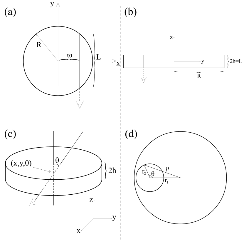
Here we focus on the RMs through a galaxy other than the Milky Way from extragalactic sources, and leave the discussion of pulsar RMs in the Milky way for section 6.5. We also omit any influence of weak intergalactic magnetic fields. The relevant segment of integration is then the segment of each line of sight $L(R,r,h)$ inside the galaxy [see figure 1 with an (a) edge-on view, (b) face-on view, and (c) inclined view], where $L$ is a function of the galactic radius $R$, the distance $r$ from the line of sight to the galactic center, and the semi-thickness of the galactic disk $h$.

In what follows, we use the subscript $L$ for a constant thermal electron density FR-like average along path $L$. For a given vector field $\bm{Q}$ and scalar field $f$ this line of sight average gives

$$(Q)_{L}=\frac{1}{L}\int d\bm{s}\cdot\bm{Q}\ {\rm and}\ (f)_{L}=\frac{1}{L}\int ds\ f.$$ (64)

For FR measurements the line-of-sight average $(\cdot)_{L}$ will thus correspond to $(\cdot)_{\mathcal{M}}$ mentioned above. We denote the theoretical prediction of the line-of-sight mean field from MFE as $(\overline{B})_{L}$. While $\sigma^{2}_{\text{IE}}$ of $(\overline{B})_{L}$ can be computed by propagating the IE of $\overline{\bm{B}}$, the FE $\sigma^{2}_{\text{FE}}$ arises from calculating the difference $(b)_{L}$, between $(\overline{B})_{L}$ and $(B)_{L}$, the latter determined by how the RMs are measured. We have

$$(b)_{L}\equiv(B)_{L}-({\overline{B}})_{L}=\frac{1}{L}\int d\bm{s}\cdot\bm{B}-\frac{1}{L}\int d\bm{s}\cdot\overline{\bm{B}}=\frac{1}{L}\int d\bm{s}\cdot\bm{b}.$$ (65)

This represents the line-of-sight mean of a fluctuation and is the deviation that results from comparing single average to a mixed double average $(q)_{\mathcal{M}}$, discussed in section 4. Here $(\overline{Q})_{\mathcal{M}}=({\overline{B}})_{L}=\frac{1}{L}\int d\bm{s}\cdot\overline{\bm{B}}$.

Our mission is to express $\sigma^{2}_{\text{IE}}$ and $\sigma^{2}_{\text{FE}}=\left\langle{(b)_{L}^{2}}\right\rangle$ in terms of known or derivable quantities for a MFT. Equation (61) gives the general form of $\sigma^{2}_{\text{IE}}$ for $\overline{\bm{B}}$. If fluctuations in different directions are uncorrelated, the intrinsic error of $(\overline{B})_{L}$ can be approximated by

$$\sigma^{2}_{\text{IE}}\simeq\frac{1}{L}\int ds\ \left[(\sigma_{\overline{B}_{x}}\hat{\bm{x}}\cdot\hat{\bm{s}})^{2}+(\sigma_{\overline{B}_{y}}\hat{\bm{y}}\cdot\hat{\bm{s}})^{2}+(\sigma_{\overline{B}_{z}}\hat{\bm{z}}\cdot\hat{\bm{s}})^{2}\right],$$ (66)

where fluctuation scales are less than $L$, which is true away from the galactic edge.

To compute $\left\langle{(b)_{L}^{2}}\right\rangle$ we assume a statistically isotropic turbulent field $\bm{b}(\bm{x})$, and therefore the integrand on the RHS in equation (65) is insensitive to the direction of the line of sight. We use a scalar $b_{\text{s}}(x)$ to represent the component of $\bm{b}(\bm{x})$ along the line of sight. Next, we assume $b_{\text{s}}(x)$ can be decomposed into different modes with specific wavelengths indicated by a superscript $(m)$, namely

$$b_{\text{s}}(x)=\sum_{m}b^{(m)}(x),$$ (67)

with $k_{m}$ being the characteristic wavenumber of each mode and satisfying

$$\frac{2\pi}{k_{m}}\leq l,$$ (68)

since the turbulent scale is smaller than the averaging scale. Correspondingly, for each mode $b^{(m)}$, we divide $L$ evenly into $n_{m}=k_{m}L/\pi$ cells. For most lines of sight, $n_{m}$ is greater than $L/l$ since roughly the largest mode has a wavelength no larger than $l$. The length of the line of sight inside the galaxy will typically be of order $l_{\text{L}}$, the characteristic scale of a large-scale magnetic field, except when observations are made edge-on and close to the galactic outer edge. Therefore, if we assume that $L/l>1$, we have $n_{m}>1$. Large $n_{m}$ will allow more accurate application of the CLT.

In each separate cell of scale $\pi/k_{m}$, $b^{(m)}$ is nearly coherent in space with the same sign, parallel or anti-parallel to $d\bm{s}$. We can then replace $b^{(m)}$ by its root-mean-square value $b_{m}$ defined by a MFE-appropriate average (section 2.4), supplemented by a ‘+’ sign if parallel to $d\bm{r}$, and a ‘-’ sign if anti-parallel. Then equation (65) becomes the sum of $m$ averages, each being the mean of $n_{m}$ random variables $b^{(m)}_{i}$, taking a value $b_{m}$ or $-b_{m}$:

$$b_{L}=\frac{1}{L}\int d\bm{s}\cdot\bm{b}=\frac{1}{L}\sum_{m}\int ds\ b^{(m)}=\sum_{m}\frac{1}{n_{m}}\sum_{i=1}^{n_{m}}b^{(m)}_{i}.$$ (69)

Although $b^{(m)}_{i}$ is likely to be correlated with both its spectral neighbor $b^{(m+1)}_{i}$ and spatial neighbor $b^{(m)}_{i+1}$ because the turbulent fields are entangled locally in both configuration and Fourier space, we assume that every $b^{(m)}_{i}$ varies independently and leave generalizations for future work.

For $n_{m}\gg 1$ the scale separation is large and $\sum_{i}b^{(m)}_{i}/n_{m}$ is close to a normally distributed random variable with zero mean and variance $b_{m}^{2}/n_{m}$. Then $b_{L}$ is the sum of $m$ independent normally distributed random variables and thus a random variable itself, with variance (Ruzmaikin et al., 1988, p. 256)

$$\sigma^{2}_{\text{FE}}=\sum_{m}\frac{b_{m}^{2}}{n_{m}}=\frac{1}{L}\sum_{m}\frac{\pi b_{m}^{2}}{k_{m}}.$$ (70)

The summation on the RHS in equation (70) is the energy density-weighted average wavelength up to a constant. The relation to energy density is somewhat of a coincidence arising because both energy and variance are related to $\left\langle{{b^{(m)}}^{2}}\right\rangle$.

The variance is more useful in its integral form. Let ${\underaccent{\sim}{M}}(k)$ be the energy spectrum of the total magnetic field. In general, $\underaccent{\sim}{M}(k)$ could vary in space, but for line-of-sight measurements, the energy spectrum averaged over the line of sight is a reasonable approximation. The energy spectra of large- and small-scale fields are then $|{\underaccent{\sim}{G}}_{l}(\bm{k})|^{2}\underaccent{\sim}{M}(k)$ and $|1-{\underaccent{\sim}{G}}_{l}(\bm{k})|^{2}\underaccent{\sim}{M}(k)$, respectively. Hence $b_{m}^{2}$ is related to the energy spectrum through

$$\frac{b_{m}^{2}}{8\pi}=|1-{\underaccent{\sim}{G}}_{l}(\bm{k}_{m})|^{2}{\underaccent{\sim}{M}}(k_{m})dk_{m},$$ (71)

given that ${\underaccent{\sim}{G}}_{l}$ is isotropic. Using this and the integral version of equation (70), we obtain

$$\sigma^{2}_{\text{FE}}=\frac{8\pi^{2}}{L}\int_{0}^{k_{\nu}}dk\ \frac{|1-{\underaccent{\sim}{G}}_{l}(\bm{k})|^{2}{\underaccent{\sim}{M}}(k)}{k}=\frac{8\pi^{2}}{k_{\text{int}}L}\int_{0}^{k_{\nu}}dk\ |1-{\underaccent{\sim}{G}}_{l}(\bm{k})|^{2}{\underaccent{\sim}{M}}(k),$$ (72)

where $k_{\nu}=2\pi/l_{\nu}$ is the wavenumber of the dissipation scale, and we have defined

$$k_{\text{int}}\equiv\frac{\int_{0}^{k_{\nu}}dk\ |1-{\underaccent{\sim}{G}}_{l}(\bm{k})|^{2}{\underaccent{\sim}{M}}(k)}{\int_{0}^{k_{\nu}}dk\ |1-{\underaccent{\sim}{G}}_{l}(\bm{k})|^{2}{\underaccent{\sim}{M}}(k)/k}$$ (73)

to be the integral scale of fluctuations which depends weakly on $l$ but roughly equals $\pi/l_{\text{s}}$, since $l_{\text{s}}$ is the coherent scale and the wavelength corresponding to it will be $2l_{\text{s}}$.

Equation (72) reveals that $\sigma^{2}_{\text{FE}}$ is proportional to the total magnetic energy in fluctuations, and the ratio between $\pi/k_{\text{int}}\simeq l_{\text{s}}$ and the segment length $L$ through the source. Equation (72) is testable with simulations. The ensemble associated with the standard deviation on its LHS could be realized by taking snapshots of the system at different times (which would equate the time average to an ensemble average), whereas the integral on the RHS is measurable in Fourier space.

To illustrate the use of equation (72), we assume $\pi/k_{\text{int}}=l_{\text{s}}$ and define

$$q_{l}=\frac{\int_{0}^{k_{\nu}}dk\ |1-{\underaccent{\sim}{G}}_{l}|^{2}\underaccent{\sim}{M}}{\int_{0}^{k_{\nu}}dk\ {\underaccent{\sim}{G}}_{l}^{2}\underaccent{\sim}{M}}$$ (74)

as the proportionality between small and large scale magnetic energies. The $q_{l}$ is independent of location along each line of sight but depends upon how we define large- and small-scale fields, through $l$ and $G_{l}$. Hence equation (72) yields

$$\sigma^{2}_{\text{FE}}=\frac{l_{\text{s}}}{L}\left(\frac{\int dk\ |1-{\underaccent{\sim}{G}}_{l}|^{2}\underaccent{\sim}{M}}{\int dk\ {\underaccent{\sim}{G}}_{l}^{2}\underaccent{\sim}{M}}\right)\left(8\pi\int dk\ {\underaccent{\sim}{G}}_{l}^{2}\underaccent{\sim}{M}\right)=\frac{l_{\text{s}}}{L}q_{l}(\overline{B}^{2})_{L}$$ (75)

where in the last equality, $(\overline{B}^{2})_{L}/8\pi=\int dk\ {\underaccent{\sim}{G}}_{l}^{2}\underaccent{\sim}{M}$, the line-of-sight average of the large-scale field energy. Note that $(\overline{B}^{2})_{L}$ is distinct from $(\overline{B}_{L})^{2}$ as the latter is the square of the line-of-sight average [see equation (64) of the theoretically predicted mean field $\overline{\bm{B}}$].

To express $q_{l}$ in terms of $l$, we assume that $l_{\text{s}}$ and $l_{\text{L}}$ are insensitive to $l$. We have checked that this is justified if, regardless of shape, $\underaccent{\sim}{M}(k)$ has two peaks, one near $k=k_{\text{L}}=2\pi/l_{\text{L}}$ and one near $k=k_{\text{s}}=2\pi/l_{\text{s}}$, and is small near $k=k_{l}$. We also define $q\equiv\left\langle{b^{2}}\right\rangle/\left\langle{B}\right\rangle^{2}$ as the proportionality between the unfiltered small- and large-scale magnetic fields [= ratio of areas under the two peaks of $\underaccent{\sim}{M}(k)$]. Observations indicate that $q$ is on average somewhere between 3 and 4 (Fletcher, 2010; Van Eck et al., 2015; Beck, 2016); we adopt a fiducial value $q=4$. Consequently, we have

$$q_{l}= \frac{\int dk\ |1-{\underaccent{\sim}{G}}_{l}|^{2}\underaccent{\sim}{M}}{\int dk\ |{\underaccent{\sim}{G}}_{l}|^{2}\underaccent{\sim}{M}}$$

$$\simeq \frac{|1-{\underaccent{\sim}{G}}_{l}(k_{\text{L}})|^{2}\left\langle{B}\right\rangle^{2}+|1-{\underaccent{\sim}{G}}_{l}(k_{\text{s}})|^{2}\left\langle{b^{2}}\right\rangle}{|{\underaccent{\sim}{G}}_{l}(k_{\text{L}})|^{2}\left\langle{B}\right\rangle^{2}+|{\underaccent{\sim}{G}}_{l}(k_{\text{s}})|^{2}\left\langle{b^{2}}\right\rangle}$$

$$= \frac{|1-{\underaccent{\sim}{G}}_{l}(k_{\text{L}})|^{2}+|1-{\underaccent{\sim}{G}}_{l}(k_{\text{s}})|^{2}q}{|{\underaccent{\sim}{G}}_{l}(k_{\text{L}})|^{2}+|{\underaccent{\sim}{G}}_{l}(k_{\text{s}})|^{2}q}.$$ (76)

Combining equations (75) and (76) we have

$$\sigma^{2}_{\text{FE}}=\frac{l_{\text{s}}}{L}q_{l}(\overline{B}^{2})_{L}=\frac{l_{\text{s}}}{L}\frac{|1-{\underaccent{\sim}{G}}_{l}(k_{\text{L}})|^{2}+|1-{\underaccent{\sim}{G}}_{l}(k_{\text{s}})|^{2}q}{|{\underaccent{\sim}{G}}_{l}(k_{\text{L}})|^{2}+|{\underaccent{\sim}{G}}_{l}(k_{\text{s}})|^{2}q}(\overline{B}^{2})_{L}.$$ (77)

Equation (77) highlights that the variance in predicted RM is the product of three factors. First, the inverse of the number of eddy cells along the line of sight, $l_{\text{s}}/L$. Being linear in the length ratio, this can be significant even when the correction terms to the modified MFE equations are small. The MFE corrections are of order $(l/l_{\text{L}})^{c}$ [see equation (8)], so for small $l/l_{\text{L}}$ ratio or large $c$, the corrections could be small even if $\sigma^{2}_{\text{FE}}$ is significant. Second, $\sigma^{2}_{\text{FE}}$ depends on how energy is distributed between large and small-scale fields through $q_{l}$. Since a larger $l$ implies more modes are counted as small scale fields ($k\lesssim 2\pi/l$), $q_{l}$ is a monotonic function of $l$. Finally, equation (77) shows that $\sigma^{2}_{\text{FE}}$ is also proportional to the average magnetic energy density along the line of sight.

Some complexities of the true error are not considered in equation (77). First, due to local inhomogeneities (spiral arms for example), cells for each mode along a single line of sight may not be statistically identical nor have the same total amplitude of fluctuating magnetic energy as we have assumed. In equation (71) we have used the line-of-sight averaged energy spectrum $\underaccent{\sim}{M}(k)$ as an approximation and ignored spatial variation of $\left\langle{b^{2}}\right\rangle$. Second, differential rotation makes turbulent magnetic fields anisotropic in an eddy turnover time $\tau$ in the galactic mid-plane. The azimuthal fluctuation is amplified beyond the radial field such that $b_{\phi}\simeq b_{r}(1+q_{r}\Omega\tau)\simeq 2b_{r}$ with the $q_{r}\simeq 1$ for a flat rotation curve, and Rossby number $Ro=1/(\Omega\tau)\approx 1$ in spiral galaxies. Therefore, the two components $b_{r},b_{\phi}$ contribute unequally along different lines of sight, making FR measurements depend not only on $L$, but also on direction.

6 Galactic dynamo and precision for different FR viewing angles

In this section we consider specific cases to elucidate the application of the calculations of precision of mean field theories given by equations (66) and (77) in the context of FR measurements. We calculate $\sigma^{2}=\sigma^{2}_{\text{IE}}+\sigma^{2}_{\text{FE}}$ in terms of mean fields when the measured galaxy is edge-on, face-on, and inclined. We also consider the special case of measuring FR from within our own Galaxy. We use a cylindrical coordinate system centered at the galactic center with coordinates $(r,\phi,z)$ and the $z$ axis coinciding with the galactic rotation axis.

6.1 Galactic dynamo model

We augment the simplified galactic dynamo model from section 4.5 of Zhou & Blackman (2017) , where the ‘no-$z$’ approximation (Subramanian & Mestel, 1993; Moss, 1995; Phillips, 2001; Sur et al., 2007; Chamandy et al., 2014) is used. The resulting $\bm{B}$ is $r$-dependent and cylindrically symmetric (i.e., azimuthally averaged). We include the correction terms of section 3 employing a Gaussian kernel (and thus $\hat{\gamma}=-\l^{2}\nabla^{2}/8\pi^{2}$), which gives

$$\hat{\gamma}=-\frac{1}{2}\frac{l^{2}}{4\pi^{2}}\partial_{z}^{2}\to\frac{l^{2}}{32h^{2}},$$ (78)

where derivatives in the radial direction are dropped assuming the disk is thin, $h/R\ll 1$. The last relation in equation (78) follows from the ‘no-$z$’ approximation, $\partial_{z}^{2}\to-(k_{h}/4)^{2}$ where $k_{h}=2\pi/h$ (Phillips, 2001; Sur et al., 2007). To the helicity density evolution equation with flux terms (Brandenburg & Subramanian, 2005a; Subramanian & Brandenburg, 2006; Sur et al., 2007) we also add the correction terms resulting from violation of the Reynolds rules and obtain

$$\partial_{t}\alpha_{\text{m}}=-\frac{2\beta}{l_{\text{s}}^{2}}\left[\frac{(1-\hat{\gamma})(\bm{\mathcal{E}}\cdot\overline{\bm{B}})+\overline{\bm{B}}\hat{\gamma}\bm{\mathcal{E}}}{B_{eq}^{2}}+\frac{\alpha_{\text{m}}}{R_{\text{m}}}\right]-\bm{\nabla}\cdot(\alpha_{\text{m}}\overline{\bm{U}})-\beta_{d}\nabla^{2}\alpha_{\text{m}}.$$ (79)

The last term of equation (79) governs the diffusive flux and we adopt $\beta_{d}=\beta$.

With the requirement that $l<h$, we find that the $\hat{\gamma}$ correction terms produce only small changes in the dynamo model solutions and we can omit them in the later discussion of the precision error. However, the smallness of the effect on the solutions is a feature of our particular dynamo model that is exacerbated by the aforementioned ‘no-$z$’ approximation. To see this note that for our choice of $l$, $\underaccent{\sim}{\gamma}(k_{h})<1$ and the magnitude of $\hat{\gamma}$ is always less than $1/16$. The maximum value of $(\overline{B})_{L}(r)$ when $l$ is increased from $0.1h$ to $0.9h$ from the solutions changes by just $\sim 1\%$. If instead we had used the approximation that $\partial_{z}^{2}\sim-k_{h}^{2}$, there would be a $\sim 40\%$ decrease in the maximum value of $(\overline{B})_{L}(r)$ when $l$ is increased from $0.1h$ to $0.9h$ from the solutions with the correction terms. This highlights that the correction terms are not necessarily small for every model. Moreover, in the absence of any significant scale separation between large and small scale parts of the magnetic energy spectrum, the expansion of ${\underaccent{\sim}{G}}_{l}(\bm{k})$ in Eqn. (6) would itself be invalid, and corrections to the MFE would be non-perturbative.

Numerically, Shapovalov & Vishniac (2011) found, from the (uncorrected) evolution equation of small-scale helicity, that the resultant spectra of large-scale quantities are insensitive to different filtering methods, for reasonable spectra of relevant total quantities.

The steady state, non-dimensionalized dynamo equations read

$$0=\partial_{t}B_{r}= -\frac{2}{\pi}R_{\alpha}(1+\alpha_{\text{m}})B_{\phi}-\left(R_{U}+\frac{\pi^{2}}{4}\right)B_{r}$$ (80)

$$0=\partial_{t}B_{\phi}= R_{\omega}B_{r}-\left(R_{U}+\frac{\pi^{2}}{4}\right)B_{\phi}$$ (81)

$$0=\partial_{t}\alpha_{\text{m}}= -R_{U}\alpha_{\text{m}}-\frac{\beta_{d}}{\beta}\frac{\pi}{2}\alpha_{m}-C\left[(1+\alpha_{\text{m}})(B_{r}^{2}+B_{\phi}^{2})\right.$$

$$\left.+\frac{3}{8}\sqrt{\frac{-\pi(1+\alpha_{m})R_{\omega}}{R_{\alpha}}}B_{r}B_{\phi}+\frac{\alpha_{m}}{R_{m}}\right],$$ (82)

where

$$R_{\alpha}=\frac{\alpha_{\text{k}}h}{\beta},\ R_{U}=\frac{|\overline{\bm{U}}|h}{\beta},\ R_{\omega}=-\frac{h^{2}\Omega}{\beta},\ C=2\left(\frac{h}{l_{\text{s}}}\right)^{2}$$ (83)

are dimensionless parameters with a flat rotation curve $\Omega\propto 1/r$ adopted, and magnetic fields are normalized by the equipartition field strength $B_{\text{eq}}=\sqrt{4\pi\rho_{\text{f}}u^{2}}$ with $\rho_{\text{f}}$ being the fluid density. The $\alpha$-coefficients are normalized by $\alpha_{\text{k}}$. The $r$-dependence of equation (83) is described in detail in section 2.4 and equation (41) in Zhou & Blackman (2017). The approximation for the $\bm{\mathcal{E}}\cdot\overline{\bm{B}}$ term can be found in the appendix of Sur et al. (2007) or that of Chamandy et al. (2013).

Analytical expressions of $\overline{B}_{\phi}$ and $\overline{B}_{r}$ are obtainable from equations (80) to (82). The intrinsic error of $\overline{\bm{B}}(\bm{x})$ is then given by equation (61) in terms of $\sigma_{\alpha_{\text{k}}}^{2}$, $\sigma_{\beta}^{2}$ and $\sigma_{{\alpha_{\text{k}}}\beta}$. The first two are given in equation (60), where as for $\sigma_{{\alpha_{\text{k}}}\beta}$ we assume that fluctuations of $\alpha_{\text{k}}$ and $\beta$ are uncorrelated, and

$$\sigma_{{\alpha_{\text{k}}}\beta}\simeq(\sigma_{\alpha_{\text{k}}}^{2}\sigma_{\beta}^{2})^{1/2}=\sigma_{\beta}^{2}R_{\alpha}/h.$$ (84)

(For galaxies, $R_{\alpha}\simeq 1$.) At a fixed location, $\overline{\bm{B}}$ is a function of $R_{\alpha}$, $R_{U}$ and $R_{\omega}$. Therefore the partial derivatives with respect to $\alpha_{\text{k}}$ and $\beta$ can be evaluated using the chain rule,

$$\partial_{\alpha_{\text{k}}}=\frac{h}{\beta}\partial_{R_{\alpha}},\ \partial_{\beta}=-\frac{1}{\beta}\left(R_{\alpha}\partial_{R_{\alpha}}+R_{U}\partial_{R_{U}}+R_{\omega}\partial_{R_{\omega}}\right).$$ (85)

Combining equations (61), (84) and (85), we have for the intrinsic error of $\overline{B}_{i}$,

$$\sigma^{2}_{\text{IE},\overline{B}_{i}}=\frac{1}{12(l/l_{\text{s}})^{3}}\left\{\right. (\partial_{R_{\alpha}}\overline{B}_{i})^{2}R_{\alpha}^{2}+[\left(R_{\alpha}\partial_{R_{\alpha}}+R_{U}\partial_{R_{U}}+R_{\omega}\partial_{R_{\omega}}\right)\overline{B}_{i}]^{2}$$

$$\left.-2(R_{\alpha}\partial_{R_{\alpha}}\overline{B}_{i})[\left(R_{\alpha}\partial_{R_{\alpha}}+R_{U}\partial_{R_{U}}+R_{\omega}\partial_{R_{\omega}}\right)\overline{B}_{i}]\right\},$$ (86)

and that of $(\overline{B})_{L}$ is given by substituting equation (86) into equation (66), given the solutions of equations (80) to (82).

6.2 Edge-on view

We first consider a special case representing the measurement of FR of a perfectly edge-on disc galaxy with radius $R=12\ \text{kpc}$ (see the schematic diagrams of figure 1). Note that the integration path segments along the line of sight within the galaxy form chords with lengths $L(\varpi)=2\sqrt{R^{2}-\varpi^{2}}$, where $\varpi$ is the distance from the galactic center to the closest point on the chord. From the geometry of the configuration, the line of sight average is

$$\overline{B}_{L}(\varpi)=\frac{2\varpi}{L(\varpi)}\int_{0}^{L/2}dy\ \frac{\overline{B}_{\phi}(r)}{r},$$ (87)

and

$$(\overline{B}^{2})_{L}(\varpi)=\frac{2}{L(\varpi)}\int_{0}^{L/2}dy\ \overline{B}^{2}(r)$$ (88)

where $r=\sqrt{\varpi^{2}+y^{2}}$ is the radial coordinate from the galactic center. Only ${\overline{B}}_{\phi}$ contributes to $(\overline{B})_{L}$ for the edge-on view because $\overline{B}_{r}$ is mirror-symmetric about the $x$-axis and its contributions from the $y>0$ and $y<0$ regions cancel each other. The intrinsic error is given by

$$\sigma^{2}_{\text{IE}}=\frac{2\varpi^{2}}{L(\varpi)}\int_{0}^{L/2}dy\ \frac{\sigma^{2}_{\text{int},\overline{B}_{\phi}}}{r^{2}}.$$ (89)

The imprecision associated with the observation is given by equation (77) and is

$$\sigma^{2}_{\text{FE}}=\frac{2l_{\text{s}}}{L^{2}}\frac{(1-e^{-l^{2}/2l_{\text{L}}^{2}})^{2}+(1-e^{-l^{2}/2l_{\text{s}}^{2}})^{2}q}{e^{-l^{2}/l_{\text{L}}^{2}}+e^{-l^{2}/l_{\text{s}}^{2}}q}\int_{0}^{L/2}dy\ \overline{B}^{2}(r),$$ (90)

where we take $l_{\text{L}}\simeq h=0.5\ \text{kpc}$, for galactic disk semi-thickness $h$, and the variation scale of turbulent fields $l_{\text{s}}\simeq 0.1\ \text{kpc}$ is assumed to be the same for velocity and magnetic fields. Here $l_{\text{L}}\simeq h$ because $\partial_{r}\ll\partial_{z}$ in a thin disk and $h$ is the smallest natural scale of variation for the mean field. Correspondingly we take an averaging scale $0.12\leq l\leq 0.48\ \text{kpc}$.

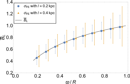
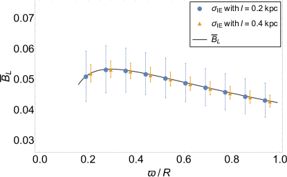
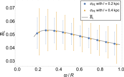
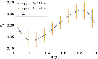
The predicted line-of-sight average of the magnetic field, together with the error bars are shown in figures 2 and 3, where two different profiles of $\bm{B}$ are separately considered: (i) in the left panel of figure 2 $\overline{\bm{B}}(\bm{x})=B_{0}\hat{\bm{\phi}}$ where $B_{0}=1$ is a constant, and (ii) in figure 3 the analytic solution of the mean field dynamo model from section 6.1, normalized by the equipartition field strength $B_{\text{eq}}=\sqrt{4\pi\rho_{\text{f}}u^{2}}$. The dimensionless parameters we have used for the analytic solution are the same as those in Zhou & Blackman (2017):

$$R_{\alpha}=R_{\alpha 0}/2,\ R_{U}=2R_{U0}/(r/r_{\odot})^{2}F^{5/2},\ R_{\omega}=2R_{\omega 0}/(r/r_{\odot})^{2}F^{3},\ C=4C_{0}/(r/r_{\odot})^{2}F^{3}$$ (91)

where quantities with subscripts $0$ are computed using

$$\tau_{\text{ed}}=10^{15}\ \text{s},\ u=10\ \text{km/s}^{-1},\ r\Omega=200\ \text{km/s}^{-1},\$$

$$l_{\text{s}}=0.1\ \text{kpc},\ h=0.5\ \text{kpc},\ U_{0}=1\ \text{km/s}^{-1},$$ (92)

which yields

$$R_{\alpha 0}=1,\ R_{U0}=0.3,\ R_{\omega 0}=-15,$$ (93)

and we use $R_{\text{m}}=10^{5}$. Above $r_{\odot}\equiv 8\ \text{kpc}$ is the location of the Sun, and the function $F$ determines the $r$-dependence of the dimensionless parameters and is described in detail in the appendix in Zhou & Blackman (2017).

The line-of-sight averages of the mean magnetic fields are shown as black solid curves, along with different types of error bars $=\pm\sigma$ about the mean computed from equations (66) and (90) for the cases associated with two different choices of the scale of average, $l$. The blue dashed lines with circular markers give error bars with $l=0.2\ \text{kpc}$, and the yellow solid lines with triangular markers give those with $l=0.4\ \text{kpc}$. In the constant magnetic field case, the intrinsic error does not exist because here $\overline{\bm{B}}$ is presumed, rather than derived from MFE equations.

Different choices of $l$ conspicuously show different levels of precision in the predictions for measurements, as evidenced by a comparison of the blue vs. yellow IE bars in the $r$-dependent model (left panel in figure 3). Variations in a data curve beneath the level of the error bars cannot be deemed a disagreement with the MFE theory. That is, whether uncorrelated or weakly correlated deviations with amplitudes below the error bars are systematic (Chamandy et al., 2016) or stochastic is beyond the resolution of the theory.

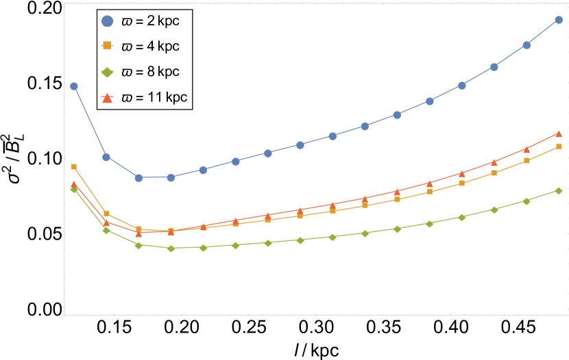
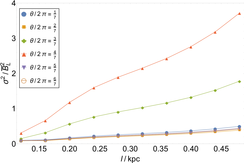
Comparing the panels of figure 3 highlights competing dependences of $\sigma^{2}_{\text{IE}}$ and $\sigma^{2}_{\text{FE}}$ on $l$, as discussed in section 4: $\sigma^{2}_{\text{IE}}$ grows with $l$ but $\sigma^{2}_{\text{FE}}$ decreases with $l$. Assuming $\sigma^{2}_{\text{IE}}$ and $\sigma^{2}_{\text{FE}}$ are independent and uncorrelated, adding them in quadrature gives the total uncertainty $\sigma^{2}$.

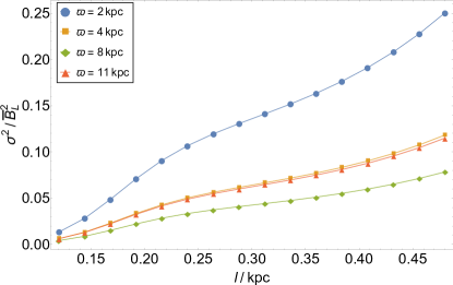
In the right panel of figure 2 and in figure 4, we show the relative total errors, $\sigma^{2}/(\overline{B})_{L}^{2}$, as a function of $0.12\ \text{kpc}\leq l\leq 0.48\ \text{kpc}$ at different galactic radii. For figure 2 there is only one uncertainty, namely $\sigma^{2}_{\text{FE}}$ which is a monotonic function of $l$ for all radii shown. More interesting case is figure 4 where both $\sigma^{2}_{\text{FE}}$ and $\sigma^{2}_{\text{IE}}$ are competitive. There is an optimal scale of average, located at $0.15\leq r/R\leq 0.20$ for all four chosen radii, that minimizes the total error, and thus maximizes the precision of comparing theory and observation. In general. the existence and location of such a ‘sweet spot’ depends on the solution to a given dynamo model, and the observational method used.

6.3 Face-on view

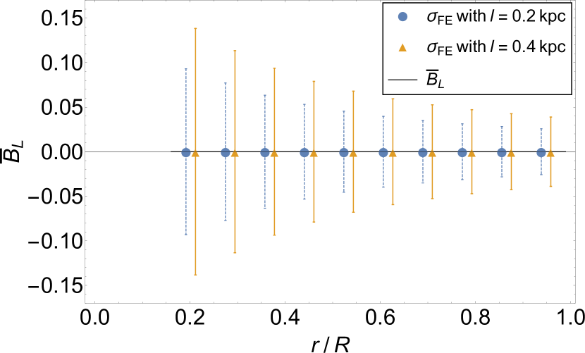
A complementary extreme to the edge-on case is a face-on view. Here every line of sight is perpendicular to the galactic disk, taken along the $z$ direction. In this orientation, $B_{\phi}$ and $B_{r}$ do not contribute to $(\overline{B})_{L}$, and for a weak ${\overline{B}}_{z}$, the dominant non-vanishing RM would come from small-scale fluctuations. If we assume quasi-equipartition between the total mean and fluctuating small scale magnetic energies, the FR measurements still predict a a precision error about which the mean field is indeterminate.

Taking $L=2h$, the thickness of the galactic disk, and noting that $\overline{\bm{B}}$ is solely a function of $r$ in equation (77), we have

$$\sigma^{2}_{\text{FE}}(r)=\frac{l_{\text{s}}}{2h}\frac{|1-{\underaccent{\sim}{G}}_{l}(k_{\text{L}})|^{2}+|1-{\underaccent{\sim}{G}}_{l}(k_{\text{s}})|^{2}q}{|{\underaccent{\sim}{G}}_{l}(k_{\text{L}})|^{2}+|{\underaccent{\sim}{G}}_{l}(k_{\text{s}})|^{2}q}(\overline{B}_{\phi}^{2}+\overline{B}_{r}^{2})_{L}.$$ (94)

Figure 5 shows $\overline{B}_{L}$ as a function of the galactic radial coordinate $r$ (normalized by the galactic radius $R$) from a face-on view of the same $r$-dependent dynamo model used in the last subsection (Zhou & Blackman, 2017). The predicted RM is now zero and its filtering error is given in blue dashed lines with circular markers for $l=0.2\ \text{kpc}$, and in yellow solid lines with triangular markers for $l=0.4\ \text{kpc}$. These emerge purely from stochastic fluctuations. The intrinsic error is zero because $\overline{B}_{z}=0$ everywhere.

6.4 Views at intermediate inclinations

The formulation becomes a bit more complicated when the line of sight is at an intermediate inclination. We adopt Cartesian coordinates in this subsection, where the $z$-axis coincides with the galactic rotation axis, $x-y$ plane coincides with the galactic mid-plane, the $y$-axis is parallel to the line of sight. Figure 1 shows a schematic plot. Let the angle between the $z$ axis and the line of sight be $\theta$, and $0<\theta<\pi/2$. The line-of-sight averages depend on the location of the intersection point of the line of sight and the galactic mid-plane, $(x,y)$, and are given by

$$(\overline{B})_{L}(x,y)=\frac{\sin\theta}{2h\sqrt{x^{2}+y^{2}}}\int_{-h}^{h}dz\ \left[x\overline{B}_{\phi}(\rho)+y\overline{B}_{r}(\rho)\right],$$ (95)

and

$$(\overline{B}^{2})_{L}(x,y)=\frac{1}{2h}\int_{-h}^{h}dz\ \overline{B}^{2}(\rho),$$ (96)

where $\rho=\sqrt{x^{2}+(z\tan\theta+y)^{2}}$. We include only the region $\{(x,y)|\rho\leq R\}$. equation (96) can then be used in equation (77) to compute the precision error associated with FR measures, and the intrinsic error is given by

$$\sigma^{2}_{\text{IE}}(x,y)=\frac{\sin^{2}\theta}{2h(x^{2}+y^{2})}\int_{-h}^{h}dz\ \left[x^{2}\sigma^{2}_{\text{int},\overline{B}_{\phi}}(\rho)+y^{2}\sigma^{2}_{\text{int},\overline{B}_{r}}(\rho)\right]$$ (97)

which can be determined once the intrinsic error of $\overline{\bm{B}}$ is calculated.

6.5 View from within our Galaxy

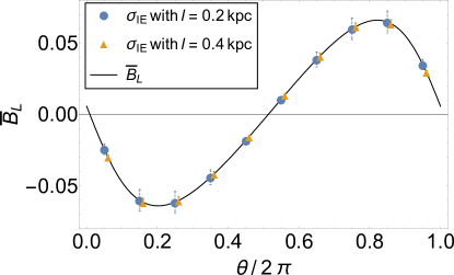
Finally, we discuss pulsar rotation measures as measured from inside our Galaxy. For simplicity, we omit the $z$-dependence and assume that both the observer and pulsars are in the Galactic mid-plane. A schematic plot is shown in figure 1. The distance of the observer to the Galactic center is denoted by $r_{1}$, and for this simple example, we assume pulsars to have a fixed distance $L=r_{2}<r_{1}$ from the observer and lie in the Galactic mid-plane. We use $r_{1}=8\text{ kpc}$ and $r_{2}=3\text{ kpc}$ for typical values in calculations. The line-of-sight average of magnetic fields is also a function of $\theta$, the azimuthal angle for a polar coordinate system centered at the earth which denotes the positions of pulsars, and $\theta=0$ points to the galactic center. The line-of-sight average of the mean field is then

$$(\overline{B})_{L}(\theta)=-\frac{r_{1}\sin\theta}{r_{2}}\int_{0}^{r_{2}}dr\ \frac{\overline{B}_{\phi}(\rho)}{\rho}+\frac{1}{r_{2}}\int_{0}^{r_{2}}dr\ \frac{r-r_{1}\cos\theta}{\rho}\overline{B}_{r}(\rho),$$ (98)

where $\rho^{2}=r_{1}^{2}-2r_{1}r\cos\theta+r^{2}$ is the radial coordinate in the galactocentric coordinate system (see figure 1). The line-of-sight averaged ${\overline{B}}^{2}$ is given by

$$(\overline{B}^{2})_{L}(\theta)=\frac{1}{r_{2}}\int_{0}^{r_{2}}dr\ \overline{B}^{2}(\rho).$$ (99)

The intrinsic error is given by

$$\sigma^{2}_{\text{IE}}(\theta)=\frac{r_{1}^{2}\sin^{2}\theta}{r_{2}}\int_{0}^{r_{2}}dr\ \frac{\sigma^{2}_{\text{IE},\overline{B}_{\phi}}}{\rho^{2}}+\frac{1}{r_{2}}\int_{0}^{r_{2}}dr\ \left(\frac{r-r_{1}\cos\theta}{\rho}\right)^{2}\sigma^{2}_{\text{IE},\overline{B}_{r}}.$$ (100)

The resultant curve is shown in figure 6 in the same plot style as those in the previous subsections. In this case, stochastic fluctuations introduce only small $\sigma^{2}_{\text{IE}}$ and moderate $\sigma^{2}_{\text{FE}}$, the latter being dominant because the line-of-sight average yields a large $(\overline{B})_{L}$ and the number of eddy cells along the line of sight is small as a consequence of small $L$. Thus $\sigma^{2}_{\text{FE}}$ dominates the total uncertainty $\sigma^{2}=\sigma^{2}_{\text{IE}}+\sigma^{2}_{\text{FE}}$, and therefore in figure 7 which again shows relative errors at different directions of observation as a function of $l$, most curves are monotonic and reach their minima when $l\rightarrow l_{\text{s}}$. Since $l$ is physically constrained in the region $[l_{\text{s}},l_{\text{L}}]$ (otherwise the statistical prescriptions of $\alpha$ and $\beta$ break down), this implies that $l\simeq l_{\text{s}}$ is the optimal choice of average scale in this case.

It cannot be excluded that for different parameters, e.g. if $q\equiv\left\langle{b^{2}}\right\rangle/\left\langle{B}\right\rangle^{2}$ were to exceed some critical value, the errors might dominate mean field variations making it difficult to statistically identify mean field reversals.

7 Conclusions

7.1 Summary

For large scale separation between mean fields and fluctuations, ensemble and spatial averages are approximately equivalent, but this is not guaranteed in many astrophysical circumstances where mesoscale fluctuations are present. With this motivation, we formally derived correction terms to MFE for spatial averaging that result from a finite scale separation. In addition, we have quantified two types of MFE precision errors: (i) the intrinsic error $\sigma^{2}_{\text{IE}}$, which can be derived by differentiating the solution of the mean field equations with respect to its input parameters and propagating the uncertainty of each parameter to the mean field; and (ii) the filtering error $\sigma^{2}_{\text{FE}}$ that results because the prediction from mean field theory is filtered differently from the observations. Specifically we considered the case where the predicted value is filtered using the kernel for the mean field and then again by the measurement kernel – whereas the observations only singly filter the full field through the measurement kernel.

We derived the MFE corrections and precision errors using convolutions of the full field and kernels, which introduce a prescribed averaging scale $l$. To realistically depict large-scale fields, the kernels must be chosen to be local in both configuration and Fourier space, and monotonically decreasing in Fourier space. We expanded the MFE equations in the ratio $l/l_{\text{L}}$, where $l_{\text{L}}$ is the dominant scale of variation of the mean field. The zeroth-order equations have the same form as those from an ensemble average, but new first-order corrections of order $(l/l_{\text{L}})^{c}$ arise due to a violation of Reynolds rules, where $c>0$ depends on the kernel. Our approach allows for moderate scale separations.

To exemplify the calculation of the precision errors, we considered contributions to (uniform density) galactic Faraday rotation measures from mesoscale fluctuations where the mean field filter is a local spatial average and the measurement kernel is a line-of-sight average. We applied the formalism to different viewing angles of a disc galaxy and find that the precision error of MFE can be large even when the corrections to the MFE equations themselves are small. This highlights the necessity of quantifying this precision of mean field theories to avoid misconstruing stochastic from systematic deviations between theory and observations. The error quantifies the predictive resolution of the theory.

Since $\sigma^{2}_{\text{IE}}$ decreases with $l$ while $\sigma^{2}_{\text{FE}}$ increases with $l$, the sum of the two errors may be non-monotonic over the physically allowed range of $l$, in turn allowing determination of optimal scale of $l$ that maximizes the precision of the theory. For example, we identified the optimal averaging scale for FR that minimizes the error to be about 0.17 kpc in our dynamo model for edge-on galactic viewing.

We also showed how our study differs from that of Rheinhardt & Brandenburg (2012) who were also motivated to address corrections to MFE equations for modest spatial scale separation. Our focus is on the influence of the kernel that enters the averaging of fields themselves whereas their focus was on the semi-empirically determined kernel relating the EMF to the mean magnetic magnetic field when the latter was defined through a planar average.

7.2 Further work

Our formalism can be tested and developed further. First, using DNS for a system that exhibits a statistically steady large-scale dynamo for a specific choice of kernel average, the saturated state from simulations could be sampled at different times and an ensemble constructed. The mean field precision error can then be measured and compared to our predictions. Second, the MFE precision calculations that we exemplified for FR could be generalized for more realistic numerical dynamo models, for comparison to observations. Generalization of the form of the magnetic spectra, allowance for spatial inhomogeneities, or calculation of still higher order corrections to MFE equations are also possible. Third, there remains analytical and numerical work to study dynamo models in which the linear order corrections to the MFE equations are not as small as those in the example models we considered with the ‘no-$z$’ formalism. For systems in which there is very little scale separation between large and small scale energy spectral peaks, going beyond our perturbative treatment of Reynolds rules violations would be necessary. The resulting generalized MFE equations in this non-perturbative regime, with correction terms that involve the full unexpanded kernel, could be solved numerically.

More broadly, analogous computations of MFE precision are warranted for comparing theory and observations for observables other than RMs such as polarized synchrotron emission in galaxies, or spectral fluxes in turbulent accretion disks. For the latter, the standard axisymmetric theory in common use is also an example of a mean field theory which is a limiting case of MFE and has a finite precision that has not yet been fully quantified (Blackman et al., 2010).

Acknowledgments: We are grateful to referee Mathias Rheinhardt for providing numerous thoroughly perceptive and detailed comments that helped us to very significantly improve the manuscript. We acknowledge support from grants NSF-AST-15156489 and HST-AR-13916 and the Laboratory for Laser Energetics at U. Rochester. EB also acknowledges the Kavli Institute for Theoretical Physics (KITP) USCB and associated support from grant NSF PHY-1125915.

Figure 1: Schematic diagrams of line-of-sight averages for calculating the precision of RM in an (a) edge-on view, (b) face-on view, (c) inclined view, and (d) inside the galaxy with $R$ being the galactic radius, $L$ the chord length along the line of sight, and $h$ the semi-thickness of the galactic disk. $\hat{\bm{\rho}}$ is the radial direction of the disk.

Figure 2: The left panel shows theoretical predictions of the line-of-sight averaged magnetic field $\overline{B}_{L}$ with the filtering error $\sigma_{\text{df}}$ shown as error bars in an edge-on view of a disc galaxy, assuming that the mean field has the form $\overline{\bm{B}}=B_{0}\hat{\bm{\phi}}$ with $B_{0}=1$. Lengths are normalized by the galactic radius $R=12\ \text{kpc}$. Two sets of error bars are shown for different choices of $l$. Right panel shows the fractional error bar values at different radii as a function of the averaging scale $l$.

Figure 3: Similar to the left panel of figure 2 but using analytic dynamo solutions for $\overline{\bm{B}}$ from section 4.5 of Zhou & Blackman (2017) by solving equations (80) to (82). The left panel shows the intrinsic error and the right panel shows the filtering error.

Figure 4: The total relative error using the analytic dynamo solutions at different radii as a function of averaging scale $l$. An optimal scale arises at 0.15-0.20 kpc which minimizes the relative error, and therefore provides the best precision of theoretical predictions.

Figure 5: Similar to figure 3 but for a face-on view of a disc galaxy, using the analytic dynamo solution.

Figure 6: Line-of-sight predictions and error bars of pulsar rotation measures for our view from within our Galaxy based on the analytically solvable dynamo model, equations (80) to (82), taken from section 4.5 in Zhou & Blackman (2017). Left and right panels show error bars corresponding to the intrinsic error and filtering error, respectively.

Figure 7: The total relative error for pulsar RMs at different azimuthal angle (centered at the earth) as a function of averaging scale $l$. Filtering error dominates as a result of short length of the line of sight.

Appendix A On the validity of equation (17)

In deriving equation (17), an approximation of $\overline{a\overline{B}}$, we have only considered the convolution of $\underaccent{\sim}{a}(\bm{k})$ and $\underaccent{\sim}{\overline{B}}(\bm{k}^{\prime})$ assuming that in this combination, only small $k=|\bm{k}|$ and $k^{\prime}=|\bm{k}^{\prime}|$ contribute. There are also contributions from other combinations of $k$ and $k^{\prime}$. In this appendix we discuss and quantify the validity of equation (17), and show that it depends primarily on the scale separation $l_{s}/L$. Specifically, we show that for a Gaussian kernel with $k_{l}=5$, equation (17) is a good approximation when $k_{\text{s}}/k_{\text{L}}\gtrsim 20$, assuming both $\underaccent{\sim}{A}(k)$ and $\underaccent{\sim}{B}(k)$ are double-peaked, and $k_{\text{s}}$ and $k_{\text{L}}$ are the characteristic wave numbers of small and large scales, respectively. In this respect, the approximation we use improves the standard theory by relaxing the assumption of infinite scale separation, but is not valid for arbitrarily small separation.

For simplicity, we focus on one-dimensional cases here. Which parts in the spectra of $a$ and $\overline{B}$ contribute most to the quantity $\overline{a\overline{B}}$ depends on the kernel, $k_{l}$, and $k_{\text{s}}/k_{\text{L}}$. We explain these dependencies in turn. The dependence on the kernel can be seen from the following. We will express $\overline{a\overline{B}}$ in $k$-space in terms of ${\underaccent{\sim}{G}}_{l}$, $\underaccent{\sim}{A}$ and $\underaccent{\sim}{B}$. First we focus on the Fourier transform of ${a\overline{B}}$, which is given by the convolution

$$(\underaccent{\sim}{a}*\overline{\underaccent{\sim}{B}})(k)=\int dk^{\prime}\ \underaccent{\sim}{a}(k^{\prime})\underaccent{\sim}{\overline{B}}(k-k^{\prime})=\int dk^{\prime}\ [1-{\underaccent{\sim}{G}}_{l}(k^{\prime})]{\underaccent{\sim}{G}}_{l}(k-k^{\prime})\underaccent{\sim}{A}(k^{\prime})\underaccent{\sim}{B}(k-k^{\prime}).$$ (101)

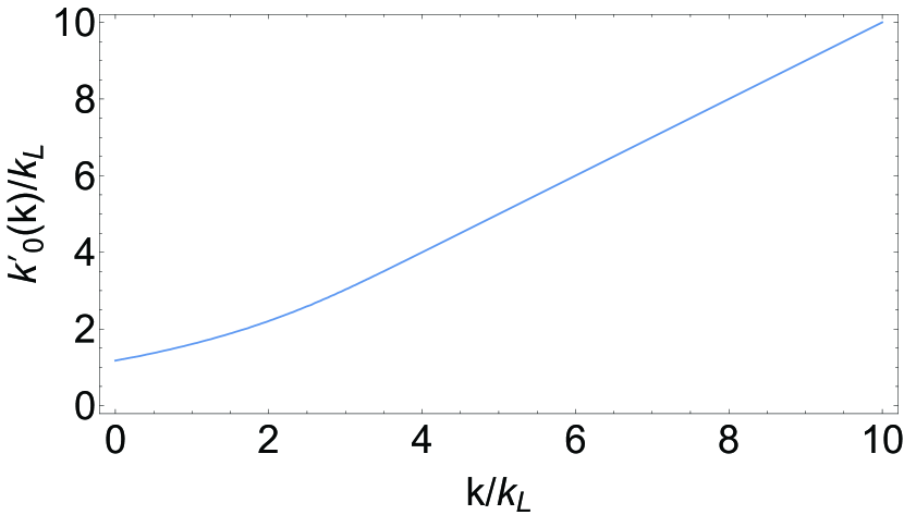
For fixed $k$, we can calculate which wavenumber $k^{\prime}$ in the convolution contributes most by differentiating the factor $[1-{\underaccent{\sim}{G}}_{l}(k^{\prime})]{\underaccent{\sim}{G}}_{l}(k-k^{\prime})$ with respect to $k^{\prime}$ and setting it to zero. The solution $k^{\prime}_{0}(k)$ depends on the form of the kernel ${\underaccent{\sim}{G}}_{l}$. How $k^{\prime}_{0}(k)$ behaves at small $k$ is of interest because we ultimately need to multiply $(\underaccent{\sim}{a*\overline{B}})(k)$ by ${\underaccent{\sim}{G}}_{l}(k)$ to get the Fourier transform of $\overline{a\overline{B}}$. If $k^{\prime}_{0}$ is small for small $k$, then we need only consider the low wavenumber parts of $a$ and $\overline{B}$ because both $k^{\prime}$ and $k-k^{\prime}$ would be small in the integrand. But $k^{\prime}_{0}$ could in general be comparable to $k_{l}$ or even larger for small $k$. For example, figure 8 shows $k^{\prime}_{0}(k)$ for a Gaussian kernel ${\underaccent{\sim}{G}}_{l}(k)=e^{-k^{2}/2k_{l}^{2}}$ with $k_{l}/k_{\text{L}}=1$. For $k\leq k_{l}$, we see that $k^{\prime}_{0}(k)$ is not small, and is of order $k_{l}$.

However, if the spectra $\underaccent{\sim}{A}(k^{\prime})$ or $\underaccent{\sim}{B}(k-k^{\prime})$ vanishes near $k^{\prime}=k^{\prime}_{0}(k)$ then the maximum contribution to equation (101) must come from other wave numbers where $\underaccent{\sim}{A}$ and $\underaccent{\sim}{B}$ are non-vanishing. In the case of double peaked spectra, with peaks at $k_{\text{L}}$ and $k_{\text{s}}$, the scale separation plays an important role in determining the significantly contributing wave numbers. In the aforementioned example of figure 8, it is possible that $\underaccent{\sim}{A}(k^{\prime})\underaccent{\sim}{B}(k-k^{\prime})$ in the integrand of equation (101) vanishes at $k^{\prime}=k^{\prime}_{0}(k)\simeq k_{l}$ for small $k$. That is, although $[1-{\underaccent{\sim}{G}}_{l}(k^{\prime})]{\underaccent{\sim}{G}}_{l}(k-k^{\prime})$ reaches its maximum at $k^{\prime}_{0}(k)$ for small $k$, $\underaccent{\sim}{A}(k^{\prime})\underaccent{\sim}{B}(k-k^{\prime})\simeq 0$ there because of large scale separation. Indeed, equation (17) is appropriate for cases with large scale separations between peaks, because the factor $[1-{\underaccent{\sim}{G}}_{l}(k^{\prime})]{\underaccent{\sim}{G}}_{l}(k-k^{\prime})$ cannot be large at small $k$ and large $k^{\prime}$. Given a fixed small $k$, this factor will vanish toward large $k^{\prime}$ and retain some non-zero value at intermediate ($\simeq k_{l}$) and small ($\lesssim k_{l}$) $k^{\prime}$ depending on the kernel. Provided there is a large enough scale separation, the intermediate $k^{\prime}$ regime does not contribute since $\underaccent{\sim}{A}$ and $\underaccent{\sim}{B}$ vanish there, leaving only the small $k^{\prime}$ part.

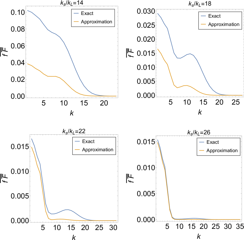
We quantify the importance of scale separation for the validity of equation (17) in figures 9 and 10 using the following double-peaked spectrum:

$$\underaccent{\sim}{F}(k)=\frac{1}{\sqrt{2\pi}\sigma_{\text{L}}}e^{-(k-k_{\text{L}})^{2}/2\sigma_{\text{L}}^{2}}+\frac{q}{\sqrt{2\pi}\sigma_{\text{s}}}e^{-(k-k_{\text{s}})^{2}/2\sigma_{\text{s}}^{2}},\ k\geq 0;\ \underaccent{\sim}{F}(k)=\underaccent{\sim}{F}(-k),\ k<0$$ (102)

where $k_{\text{L}}=1$, $\sigma_{\text{L}}=1$, $\sigma_{\text{s}}=4$ and $q=4$ are fixed. We use a Gaussian kernel for filtering, namely

$${\underaccent{\sim}{G}}_{l}(k)=e^{-k^{2}/2/k_{l}^{2}},$$ (103)

where $k_{l}=5$ is fixed. We then test equation (17) by comparing the exact result $P_{\text{e}}=\mathcal{F}[{\overline{f\overline{F}}}]=G(k)[\underaccent{\sim}{f}*\underaccent{\sim}{\overline{F}}](k)$ and its approximation $P_{\text{a}}=G(k)[\underaccent{\sim}{\overline{F}}*\underaccent{\sim}{\gamma}\underaccent{\sim}{\overline{F}}](k)$ [$\underaccent{\sim}{\gamma}$ is defined through equation (6)] for different scale separations of the peaks, as quantified by $k_{\text{s}}/k_{\text{L}}$. The comparison is shown in figure 9 where blue curves are the exact results, and yellow ones are the approximations.

The efficacy of the approximation can be quantified by the mean relative difference between blue and yellow curves in the plots figure 9, that is

$$\overline{\Delta}=\frac{\int_{0}^{k_{\nu}}dk\ \frac{P_{\text{e}}-P_{\text{a}}}{P_{\text{e}}}}{\int_{0}^{k_{\nu}}dk},$$ (104)

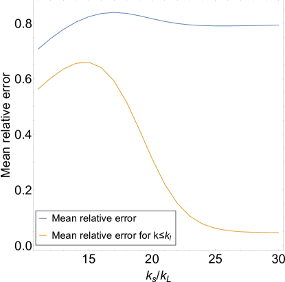
where we set $k_{\nu}=k_{\text{s}}+2\sigma_{\text{s}}$. The quantity $\overline{\Delta}$ as function of $k_{s}/k_{L}$ is shown in blue in the left panel of figure 10. It remains relatively constant over the plot, even when scale separation is large. In that case, even though the approximation agrees with the exact result at small $k$, the relative deviation from the approximation becomes large at large $k$. But since we are interested in the net value of the convolution at small $k\leq k_{l}$, a better indicator of the efficacy of the approximation is the mean relative difference at $k\leq k_{l}$; that is

$${\overline{\Delta}}_{k\leq k_{l}}=\frac{\int_{0}^{k_{l}}dk\ \frac{P_{\text{e}}-P_{\text{a}}}{P_{\text{e}}}}{\int_{0}^{k_{l}}dk}.$$ (105)

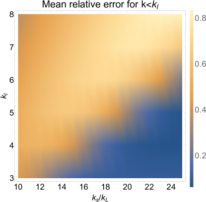
This is shown in the yellow curve in the left panel of figure 10. $P_{\text{a}}$ becomes a good approximation of $P_{\text{e}}$ when $k_{l}=5$ and $k_{\text{s}}/k_{\text{L}}\gtrsim 20$ (noting that $k_{\text{L}}=1$). In the right panel of figure 10 we plot ${\overline{\Delta}}_{k\leq k_{l}}$ but now also varying $k_{l}$ in addition to $k_{\text{s}}/k_{\text{L}}$. The scale separation required to validate equation (17) increases with increasing $k_{l}$.

Note that the dependencies of correction terms to the mean field equations of Section 3 and the efficacy of the approximation (17) on scales are different: The former depends on the ratio $k_{\text{L}}/k_{l}$, whereas the latter depends on $k_{\text{L}}/k_{\text{s}}$. In the case of large scale separation, it is therefore possible that the error of the approximations are negligible but the MFE correction terms are still significant.

Figure 8: $k^{\prime}_{0}(k)$ for a Gaussian kernel $e^{-k^{2}/2k_{l}^{2}}$ with $k_{l}=1$.

Figure 9: Comparisons of exact and approximated results of $\overline{f\overline{F}}$ for different scale separations $k_{\text{s}}/k_{\text{L}}$.

Figure 10: Left panel: The mean relative errors defined in equations (104) and (105) from comparing the exact and approximated results of $\overline{f\overline{F}}$ as a function of $k_{\text{s}}/k_{\text{L}}$. Right panel: The mean relative error for $k<k_{l}$ as a function of $k_{\text{s}}/k_{\text{L}}$ and $k_{l}$.

Appendix B Derivation of the first two terms in equation (40)

The expansion rule (22) cannot be immediately applied to the first term on the RHS of equation (38) because $\bm{b}$ does not commute with the projection operator $\hat{\bf P}$. Therefore let us write it as

$$\epsilon_{ijk}\overline{b_{k}\hat{P}_{lj}(\overline{B}_{n}\partial_{n}b_{l}+b_{n}\partial_{n}\overline{B}_{l})}= \epsilon_{ijk}\overline{b_{k}\left(\delta_{lj}-{\partial_{l}\partial_{j}}{\nabla^{-2}}\right)(\overline{B}_{n}\partial_{n}b_{l}+b_{n}\partial_{n}\overline{B}_{l})}$$

$$= \epsilon_{ijk}\overline{b_{k}\left[(\overline{B}_{n}\partial_{n}b_{j}+b_{n}\partial_{n}\overline{B}_{j})-{\partial_{j}}{\nabla^{-2}}(\partial_{l}\overline{B}_{n}\partial_{n}b_{l}+\partial_{l}b_{n}\partial_{n}\overline{B}_{l})\right]}$$

$$= \epsilon_{ijk}\overline{\overline{B}_{n}b_{k}\partial_{n}b_{j}}+\epsilon_{ijk}\overline{b_{k}b_{n}\partial_{n}\overline{B}_{j}}-2\epsilon_{ijk}\overline{b_{k}{\partial_{j}}{\nabla^{-2}}(\partial_{l}\overline{B}_{n}\partial_{n}b_{l})}.$$ (106)

The first term can be readily calculated assuming isotropy for turbulent fields, yielding

$$(1-\hat{\gamma})\left(\frac{1}{3}\overline{\bm{b}\cdot\bm{\nabla}\times\bm{b}}\ \overline{B}_{i}\right)+\overline{B}_{i}\hat{\gamma}\left(\frac{1}{3}\overline{\bm{b}\cdot\bm{\nabla}\times\bm{b}}\right).$$ (107)

Denote the third term in equation (106) by $-2X_{i}$. Then

$$X_{i}=\epsilon_{ijk}\overline{b_{k}{\partial_{j}}{\nabla^{-2}}(\partial_{l}\overline{B}_{n}\partial_{n}b_{l})}=\epsilon_{ijk}\overline{b_{k}{\nabla^{-2}}(\partial_{jl}\overline{B}_{n}\partial_{n}b_{l}+\partial_{l}\overline{B}_{n}\partial_{jn}b_{l})}.$$ (108)

The first term in the parentheses is $k_{\text{s}}/k_{\text{L}}$ times smaller than the second, and is therefore dropped. In Fourier space, the inverse of the Laplacian operator acting on the second term yields

$$\mathcal{F}[{\nabla^{-2}}(\partial_{l}\overline{B}_{n}\partial_{jn}b_{l})]=\frac{1}{k^{2}}\int d^{3}k^{\prime}\ i(k_{l}-k^{\prime}_{l})\overline{B}_{n}(\bm{k}-\bm{k}^{\prime})(k^{\prime}_{j}k^{\prime}_{n})b_{l}(\bm{k}^{\prime}).$$ (109)

$\bm{k}-\bm{k}^{\prime}$ is close to zero because of the presence of $\overline{\bm{B}}(\bm{k}-\bm{k}^{\prime})$. Therefore we expand $1/k^{2}$ as

$$\frac{1}{k^{2}}=\frac{1}{k^{\prime 2}}+\mathcal{O}(|\bm{k}-\bm{k}^{\prime}|).$$ (110)

Only the zeroth order term is kept, because terms of higher order yield derivatives of $\overline{\bm{B}}$, which makes $X_{i}$ contain second or higher order derivatives of $\overline{\bm{B}}$. Equivalently, this means the $\nabla^{-2}$ operator will not act on the $\overline{\bm{B}}$ term to this order. We now have, up to terms linear in $\overline{\bm{B}}$ or $\bm{\nabla}\overline{\bm{B}}$,

$$X_{i}\simeq\epsilon_{ijk}\overline{\partial_{l}\overline{B}_{n}b_{k}{\partial_{jn}}{\nabla^{-2}}b_{l}}$$ (111)

using equation (22).

Now the sum of the last two terms in equation (106) can be written as

$$\epsilon_{ijk}\overline{b_{k}b_{n}\partial_{n}\overline{B}_{j}}-2\epsilon_{ijk}\overline{\partial_{l}\overline{B}_{n}b_{k}{\partial_{jn}}{\nabla^{-2}}b_{l}}=(1-\hat{\gamma})\left(\partial_{l}\overline{B}_{n}\xi_{iln}\right)+\partial_{l}\overline{B}_{n}\hat{\gamma}\xi_{iln}$$ (112)

where

$$\xi_{iln}=\epsilon_{ijk}\overline{b_{k}\left(\delta_{jn}-2{\partial_{jn}}{\nabla^{-2}}\right)b_{l}}.$$ (113)

To evaluate $\xi_{iln}$, note that its Fourier transform is proportional to

$$\epsilon_{ijk}\int d^{3}k^{\prime}\ P_{kl}(k^{\prime})\left(\delta_{jn}-2\frac{k^{\prime}_{j}k^{\prime}_{n}}{k^{\prime 2}}\right)$$ (114)

since the helical part of $\overline{\underaccent{\sim}{b}_{k}\underaccent{\sim}{b}_{l}}$ ($\propto\epsilon_{pkl}k_{p}$) does not contribute. Equation (114) then gives

$$\epsilon_{ijk}\int d^{3}k^{\prime}\ \left(\delta_{kl}\delta_{jn}-2\delta_{kl}\frac{k^{\prime}_{j}k^{\prime}_{n}}{k^{\prime 2}}-\delta_{jn}\frac{k^{\prime}_{k}k^{\prime}_{l}}{k^{\prime 2}}\right)=0$$ (115)

using $\int d\Omega^{\prime}k_{i}k_{j}/k^{2}=\delta_{ij}/3$. Therefore the RHS of equation (112) is zero and altogether we have

$$\epsilon_{ijk}\overline{b_{k}\hat{P}_{lj}(\overline{B}_{n}\partial_{n}b_{l}+b_{n}\partial_{n}\overline{B}_{l})}=(1-\hat{\gamma})\left(\frac{1}{3}\overline{\bm{b}\cdot\bm{\nabla}\times\bm{b}}\ \overline{B}_{i}\right)+\overline{B}_{i}\hat{\gamma}\left(\frac{1}{3}\overline{\bm{b}\cdot\bm{\nabla}\times\bm{b}}\right).$$ (116)

References

- Aluie (2017) Aluie, H. 2017 Coarse-grained incompressible magnetohydrodynamics: analyzing the turbulent cascades. New Journal of Physics 19 (2), 025008.
- Aluie & Eyink (2010) Aluie, H. & Eyink, G. L. 2010 Scale Locality of Magnetohydrodynamic Turbulence. Physical Review Letters 104 (8), 081101.
- Beck (2016) Beck, R. 2016 Magnetic fields in spiral galaxies. Astron. Astrophys. Rev. 24, 4.
- Bhat et al. (2016) Bhat, P., Ebrahimi, F. & Blackman, E. G. 2016 Large-scale dynamo action precedes turbulence in shearing box simulations of the magnetorotational instability. MNRAS 462, 818–829.
- Blackman (2000) Blackman, E. G. 2000 Mean Magnetic Field Generation in Sheared Rotators. ApJ 529, 138–145.
- Blackman (2015) Blackman, E. G. 2015 Magnetic Helicity and Large Scale Magnetic Fields: A Primer. Sp Sci. Rev. 188, 59–91.
- Blackman & Field (2002) Blackman, E. G. & Field, G. B. 2002 New Dynamical Mean-Field Dynamo Theory and Closure Approach. Physical Review Letters 89 (26), 265007.
- Blackman & Nauman (2015) Blackman, E. G. & Nauman, F. 2015 Motivation and challenge to capture both large-scale and local transport in next generation accretion theory. Journal of Plasma Physics 81 (5), 395810505.
- Blackman et al. (2010) Blackman, E. G., Nauman, F. & Edgar, R. G. 2010 Quantifying the Imprecision of Accretion Theory and Implications for Multi-Epoch Observations of Protoplanetary Discs. ArXiv e-prints .
- Brandenburg (2009) Brandenburg, A. 2009 The critical role of magnetic helicity in astrophysical large-scale dynamos. Plasma Physics and Controlled Fusion 51 (12), 124043.
- Brandenburg et al. (2008) Brandenburg, A., Rädler, K.-H. & Schrinner, M. 2008 Scale dependence of alpha effect and turbulent diffusivity. A&A 482, 739–746.
- Brandenburg & Subramanian (2005a) Brandenburg, A. & Subramanian, K. 2005a Astrophysical magnetic fields and nonlinear dynamo theory. Physics Reports 417, 1–209.
- Brandenburg & Subramanian (2005b) Brandenburg, A. & Subramanian, K. 2005b Minimal tau approximation and simulations of the alpha effect. A&A 439, 835–843.
- Burn (1966) Burn, B. J. 1966 On the depolarization of discrete radio sources by Faraday dispersion. MNRAS 133, 67.
- Chamandy (2016) Chamandy, L. 2016 An analytical dynamo solution for large-scale magnetic fields of galaxies. MNRAS 462, 4402–4415.
- Chamandy et al. (2014) Chamandy, L., Shukurov, A., Subramanian, K. & Stoker, K. 2014 Non-linear galactic dynamos: a toolbox. MNRAS 443, 1867–1880.
- Chamandy et al. (2016) Chamandy, L., Shukurov, A. & Taylor, A. R. 2016 Statistical Tests of Galactic Dynamo Theory. ApJ 833, 43.
- Chamandy et al. (2013) Chamandy, L., Subramanian, K. & Shukurov, A. 2013 Galactic spiral patterns and dynamo action - I. A new twist on magnetic arms. MNRAS 428, 3569–3589.
- Dakhoul & Bedford (1986a) Dakhoul, V. M. & Bedford, K. W. 1986a Improved averaging method for turbulent flow simulation. I - Theoretical development and application to Burgers’ transport equation. II - Calculations and verification. International Journal for Numerical Methods in Fluids 6, 49–82.
- Dakhoul & Bedford (1986b) Dakhoul, Y. M. & Bedford, K. W. 1986b Improved averaging method for turbulent flow simulation. Part II: Calculations and verification. International Journal for Numerical Methods in Fluids 6, 65–82.
- Eilek (1989a) Eilek, J. A. 1989a Turbulence in extended synchrotron radio sources. I - Polarization of turbulent sources. II - Power-spectral analysis. AJ 98, 244–266.
- Eilek (1989b) Eilek, J. A. 1989b Turbulence in Extended Synchrotron Radio Sources. II. Power-Spectral Analysis. AJ 98, 256.
- Eyink & Aluie (2009) Eyink, G. L. & Aluie, H. 2009 Localness of energy cascade in hydrodynamic turbulence. I. Smooth coarse graining. Physics of Fluids 21 (11), 115107–115107.
- Fletcher (2010) Fletcher, A. 2010 Magnetic Fields in Nearby Galaxies. In The Dynamic Interstellar Medium: A Celebration of the Canadian Galactic Plane Survey (ed. R. Kothes, T. L. Landecker & A. G. Willis), Astronomical Society of the Pacific Conference Series, vol. 438, p. 197.
- Frick et al. (2001) Frick, P., Beck, R., Berkhuijsen, E. M. & Patrickeyev, I. 2001 Scaling and correlation analysis of galactic images. MNRAS 327, 1145–1157.
- Frisch et al. (1975) Frisch, U., Pouquet, A., Leorat, J. & Mazure, A. 1975 Possibility of an inverse cascade of magnetic helicity in magnetohydrodynamic turbulence. Journal of Fluid Mechanics 68, 769–778.
- Gent et al. (2013) Gent, F. A., Shukurov, A., Sarson, G. R., Fletcher, A. & Mantere, M. J. 2013 The supernova-regulated ISM - II. The mean magnetic field. MNRAS 430, L40–L44.
- Germano (1992) Germano, M. 1992 Turbulence - The filtering approach. Journal of Fluid Mechanics 238, 325–336.
- Germano et al. (1991) Germano, M., Piomelli, U., Moin, P. & Cabot, W. H. 1991 A dynamic subgrid-scale eddy viscosity model. Physics of Fluids A 3, 1760–1765.
- Hubbard & Brandenburg (2009) Hubbard, A. & Brandenburg, A. 2009 Memory Effects in Turbulent Transport. ApJ 706, 712–726.
- Hubbard & Brandenburg (2011) Hubbard, A. & Brandenburg, A. 2011 Magnetic Helicity Flux in the Presence of Shear. ApJ 727, 11.
- Kleeorin & Rogachevskii (2008) Kleeorin, N. & Rogachevskii, I. 2008 Mean-field dynamo in a turbulence with shear and kinetic helicity fluctuations. Physical Review E 77 (3), 036307.
- Kleeorin et al. (2009) Kleeorin, N., Rogachevskii, I., Sokoloff, D. & Tomin, D. 2009 Mean-field dynamos in random Arnold-Beltrami-Childress and Roberts flows. Physical Review E 79 (4), 046302.
- Kraichnan (1973) Kraichnan, R. H. 1973 Helical turbulence and absolute equilibrium. Journal of Fluid Mechanics 59, 745–752.
- Krause & Rädler (1980) Krause, F. & Rädler, K.-H. 1980 Mean-field magnetohydrodynamics and dynamo theory.
- Leonard (1974) Leonard, A. 1974 Energy Cascade in Large-Eddy Simulations of Turbulent Fluid Flows. Advances in Geophysics 18, 237.
- Lilly (1992) Lilly, D. K. 1992 A proposed modification of the Germano subgrid-scale closure method. Physics of Fluids A 4, 633–635.
- Meneveau & Katz (2000) Meneveau, Charles & Katz, Joseph 2000 Scale-invariance and turbulence models for large-eddy simulation. Annual Review of Fluid Mechanics 32 (1), 1–32.
- Moss (1995) Moss, D. 1995 On the generation of bisymmetric magnetic field structures in spiral galaxies by tidal interactions. MNRAS 275, 191–194.
- Moss et al. (2008) Moss, D., Sokoloff, D., Usoskin, I. & Tutubalin, V. 2008 Solar Grand Minima and Random Fluctuations in Dynamo Parameters. Solar Physics 250, 221–234.
- Phillips (2001) Phillips, A. 2001 A comparison of the asymptotic and no-z approximations for galactic dynamos. Geophysical and Astrophysical Fluid Dynamics 94, 135–150.
- Pouquet et al. (1976) Pouquet, A., Frisch, U. & Leorat, J. 1976 Strong MHD helical turbulence and the nonlinear dynamo effect. Journal of Fluid Mechanics 77, 321–354.
- Rädler (2000) Rädler, K.-H. 2000 The Generation of Cosmic Magnetic Fields. In From the Sun to the Great Attractor (ed. D. Page & J. G. Hirsch), Lecture Notes in Physics, Berlin Springer Verlag, vol. 556, p. 101.
- Rädler & Rheinhardt (2007) Rädler, K.-H. & Rheinhardt, M. 2007 Mean-field electrodynamics: critical analysis of various analytical approaches to the mean electromotive force. Geophysical and Astrophysical Fluid Dynamics 101, 117–154.
- Rheinhardt & Brandenburg (2012) Rheinhardt, M. & Brandenburg, A. 2012 Modeling spatio-temporal nonlocality in mean-field dynamos. Astronomische Nachrichten 333, 71–77.
- Roberts & Soward (1975) Roberts, P. H. & Soward, A. M. 1975 A unified approach to mean field electrodynamics. Astronomische Nachrichten 296, 49–64.
- Ruzmaikin et al. (1988) Ruzmaikin, A. A., Sokoloff, D. D. & Shukurov, A. M., ed. 1988 Magnetic fields of galaxies, Astrophysics and Space Science Library, vol. 133.
- Shapovalov & Vishniac (2011) Shapovalov, D. S. & Vishniac, E. T. 2011 Simulations of Turbulent Dynamos Driven by the Magnetic Helicity Flux. ApJ 738, 66.
- Shebalin (1989) Shebalin, J. V. 1989 Broken ergodicity and coherent structure in homogeneous turbulence. Physica D Nonlinear Phenomena 37, 173–191.
- Shebalin (2010) Shebalin, J. V. 2010 Broken ergodicity in two-dimensional homogeneous magnetohydrodynamic turbulence. Physics of Plasmas 17 (9), 092303.
- Shebalin (2013) Shebalin, J. V. 2013 Broken ergodicity in magnetohydrodynamic turbulence. Geophysical and Astrophysical Fluid Dynamics 107, 411–466.
- Smagorinsky (1963) Smagorinsky, J. 1963 General Circulation Experiments with the Primitive Equations. Monthly Weather Review 91, 99.
- Sokoloff et al. (1998) Sokoloff, D. D., Bykov, A. A., Shukurov, A., Berkhuijsen, E. M., Beck, R. & Poezd, A. D. 1998 Depolarization and Faraday effects in galaxies. MNRAS 299, 189–206.
- Spangler (1982) Spangler, S. R. 1982 The transport of polarized synchrotron radiation in a turbulent medium. ApJ 261, 310–320.
- Subramanian & Brandenburg (2006) Subramanian, K. & Brandenburg, A. 2006 Magnetic Helicity Density and Its Flux in Weakly Inhomogeneous Turbulence. ApJL 648, L71–L74.
- Subramanian & Mestel (1993) Subramanian, K. & Mestel, L. 1993 Galactic Dynamos and Density Wave Theory - Part Two - an Alternative Treatment for Strong Non-Axisymmetry. MNRAS 265, 649.
- Sur et al. (2007) Sur, S., Shukurov, A. & Subramanian, K. 2007 Galactic dynamos supported by magnetic helicity fluxes. MNRAS 377, 874–882.
- Tribble (1991) Tribble, P. C. 1991 Radio emission in a random magnetic field - Radio haloes and the structure of the magnetic field in the Coma cluster. MNRAS 253, 147–152.
- Van Eck et al. (2015) Van Eck, C. L., Brown, J. C., Shukurov, A. & Fletcher, A. 2015 Magnetic Fields in a Sample of Nearby Spiral Galaxies. ApJ 799, 35.
- Yeo (1987) Yeo, Woon Kwang 1987 A generalized high pass/low pass averaging procedure for deriving and solving turbulent flow equations. PhD thesis, The Ohio State University.
- Yoshizawa & Yokoi (1993) Yoshizawa, A. & Yokoi, N. 1993 Turbulent magnetohydrodynamic dynamo for accretion disks using the cross-helicity effect. ApJ 407, 540–548.
- Zhou & Blackman (2017) Zhou, H. & Blackman, E. G. 2017 Some consequences of shear on galactic dynamos with helicity fluxes. MNRAS 469, 1466–1475.