An Elementary Introduction to Kalman Filtering

Abstract.

Kalman filtering is a classic state estimation technique used in application areas such as signal processing and autonomous control of vehicles. It is now being used to solve problems in computer systems such as controlling the voltage and frequency of processors.

Although there are many presentations of Kalman filtering in the literature, they usually deal with particular systems like autonomous robots or linear systems with Gaussian noise, which makes it difficult to understand the general principles behind Kalman filtering. In this paper, we first present the abstract ideas behind Kalman filtering at a level accessible to anyone with a basic knowledge of probability theory and calculus, and then show how these concepts can be applied to the particular problem of state estimation in linear systems. This separation of concepts from applications should make it easier to understand Kalman filtering and to apply it to other problems in computer systems.

1. Introduction

Kalman filtering is a state estimation technique invented in 1960 by Rudolf E. Kálmán (Kalman, 1960). Because of its ability to extract useful information from noisy data and its small computational and memory requirements, it is used in many application areas including spacecraft navigation, motion planning in robotics, signal processing, and wireless sensor networks (Souza et al., 2016; Nagarajan et al., 2011; Thrun et al., 2005; Welch and Bishop, 1995; Hess and Rantzer, 2010). Recent work has used Kalman filtering in controllers for computer systems (Bergman, 2009; Pothukuchi et al., 2016; Imes and Hoffmann, 2016; Imes et al., 2015).

Although many introductions to Kalman filtering are available in the literature (Barker et al., 1994; Welch and Bishop, 1995; Balakrishnan, 1987; Eubank, 2005; Grewal and Andrews, 2014; Evensen, 2006; Faragher, 2012; Chui and Chen, 2017; Lindquist and Picci, 2017; Nakamura et al., 2007; Cao and Schwartz, 2004; Becker, 2018; Rhudy et al., 2017; Babb, 2018), they are usually focused on particular applications like robot motion or state estimation in linear systems. This can make it difficult to see how to apply Kalman filtering to other problems. Other presentations derive Kalman filtering as an application of Bayesian inference assuming that noise is Gaussian. This leads to the common misconception that Kalman filtering can be applied only if noise is Gaussian (Julier and Uhlmann, 2004). The goal of this paper is to present the abstract concepts behind Kalman filtering in a way that is accessible to most computer scientists while clarifying the key assumptions, and then show how the problem of state estimation in linear systems can be solved as an application of these general concepts.

Abstractly, Kalman filtering can be seen as a particular approach to combining approximations of an unknown value to produce a better approximation. Suppose we use two devices of different designs to measure the temperature of a CPU core. Because devices are usually noisy, the measurements are likely to differ from the actual temperature of the core. Since the devices are of different designs, let us assume that noise affects the two devices in unrelated ways (this is formalized using the notion of correlation in Section 2). Therefore, the measurements $x_{1}$ and $x_{2}$ are likely to be different from each other and from the actual core temperature $x_{c}$. A natural question is the following: is there a way to combine the information in the noisy measurements $x_{1}$ and $x_{2}$ to obtain a good approximation of the actual temperature $x_{c}$?

One ad hoc solution is to use the formula $0.5{*}x_{1}{+}0.5{*}x_{2}$ to take the average of the two measurements, giving them equal weight. Formulas of this sort are called linear estimators because they use a weighted sum to fuse values; for our temperature problem, their general form is $\beta{*}x_{1}{+}\alpha{*}x_{2}$. In this paper, we use the term estimate to refer to both a noisy measurement and to a value computed by an estimator, since both are approximations of unknown values of interest.

Suppose we have additional information about the two devices; say the second one uses more advanced temperature sensing. Since we would have more confidence in the second measurement, it seems reasonable that we should discard the first one, which is equivalent to using the linear estimator $0.0{*}x_{1}+1.0{*}x_{2}$. Kalman filtering tells us that in general, this intuitively reasonable linear estimator is not “optimal”; paradoxically, there is useful information even in the measurement from the lower-quality device, and the optimal estimator is one in which the weight given to each measurement is proportional to the confidence we have in the device producing that measurement. Only if we have no confidence whatever in the first device should we discard its measurement.

Section 2 describes how these intuitive ideas can be quantified. Estimates are modeled as random samples from distributions, and confidence in estimates is quantified in terms of the variances and covariances of these distributions. Sections 3-5 develop the two key ideas behind Kalman filtering.

1. How should estimates be fused optimally?

   Section 3 shows how to fuse scalar estimates such as temperatures optimally. It is also shown that the problem of fusing more than two estimates can be reduced to the problem of fusing two estimates at a time without any loss in the quality of the final estimate.

   Section 4 extends these results to estimates that are vectors, such as state vectors representing the estimated position and velocity of a robot.

2. In some applications, estimates are vectors but only a part of the vector can be measured directly. For example, the state of a spacecraft may be represented by its position and velocity, but only its position may be observable. In such situations, how do we obtain a complete estimate from a partial estimate?

   Section 5 shows how the Best Linear Unbiased Estimator (BLUE) can be used for this. Intuitively, it is assumed that there is a linear relationship between the observable and hidden parts of the state vector, and this relationship is used to compute an estimate for the hidden part of the state, given an estimate for the observable part.

Section 6 uses these ideas to solve the state estimation problems for linear systems, which is the usual context for presenting Kalman filters. Section 7 briefly discusses extensions of Kalman filtering for nonlinear systems.

2. Formalization of estimates

This section makes precise the notions of estimates and confidence in estimates.

2.1. Scalar estimates

Figure 1. Using pdfs to model devices with systematic and random errors. Ground truth is $60\,^{\circ}\mathrm{C}$. Dashed lines are means of pdfs.

To model the behavior of devices producing noisy measurements, we associate each device $i$ with a random variable that has a probability density function (pdf) $p_{i}(x)$ such as the ones shown in Figure 1 (the x-axis in this figure represents temperature). Random variables need not be Gaussian. Obtaining a measurement from device $i$ corresponds to drawing a random sample from the distribution for that device. We write $x_{i}{\sim}p_{i}(\mu_{i},\sigma_{i}^{2})$ to denote that $x_{i}$ is a random variable with pdf $p_{i}$ whose mean and variance are $\mu_{i}$ and $\sigma_{i}^{2}$ respectively; following convention, we use $x_{i}$ to represent a random sample from this distribution as well.

Means and variances of distributions model different kinds of inaccuracies in measurements. Device $i$ is said to have a systematic error or bias in its measurements if the mean $\mu_{i}$ of its distribution is not equal to the actual temperature $x_{c}$ (in general, to the value being estimated, which is known as ground truth); otherwise, the instrument is unbiased. Figure 1 shows pdfs for two devices that have different amounts of systematic error. The variance $\sigma_{i}^{2}$ on the other hand is a measure of the random error in the measurements. The impact of random errors can be mitigated by taking many measurements with a given device and averaging their values, but this approach will not help to reduce systematic error.

In the usual formulation of Kalman filtering, it is assumed that measuring devices do not have systematic errors. However, we do not have the luxury of taking many measurements of a given state, so we must take into account the impact of random error on a single measurement. Therefore, confidence in a device is modeled formally by the variance of the distribution associated with that device; the smaller the variance, the higher our confidence in the measurements made by the device. In Figure 1, the fact that we have less confidence in the first device has been illustrated by making $p_{1}$ more spread out than $p_{2}$, giving it a larger variance.

The informal notion that noise should affect the two devices in “unrelated ways” is formalized by requiring that the corresponding random variables be uncorrelated. This is a weaker condition than requiring them to be independent, as explained in the Appendix A. Suppose we are given the measurement made by one of the devices (say $x_{1}$) and we have to guess what the other measurement ($x_{2})$ might be. If knowing $x_{1}$ does not give us any new information about what $x_{2}$ might be, the random variables are independent. This is expressed formally by the equation $p(x_{2}|x_{1})=p(x_{2})$; intuitively, knowing the value of $x_{1}$ does not change the pdf for the possible values of $x_{2}$. If the random variables are only uncorrelated, knowing $x_{1}$ might give us new information about $x_{2}$ such as restricting its possible values but the mean of $x_{2}|x_{1}$ will still be $\mu_{2}$. Using expectations, this can be written as $E[x_{2}|x_{1}]=E[x_{2}]$, which is equivalent to requiring that $E[(x_{1}{-}\mu_{1})(x_{2}{-}\mu_{2})]$, the covariance between the two variables, be equal to zero. This is obviously a weaker condition than independence.

Although the discussion in this section has focused on measurements, the same formalization can be used for estimates produced by an estimator. Lemma 2.1(i) shows how the mean and variance of a linear combination of pairwise uncorrelated random variables can be computed from the means and variances of the random variables (Maybeck, 1982). The mean and variance can be used to quantify bias and random errors for the estimator as in the case of measurements.

An unbiased estimator is one whose mean is equal to the unknown value being estimated and it is preferable to a biased estimator with the same variance. Only unbiased estimators are considered in this paper. Furthermore, an unbiased estimator with a smaller variance is preferable to one with a larger variance since we would have more confidence in the estimates it produces. As a step towards generalizing this discussion to estimators that produce vector estimates, we refer to the variance of an unbiased scalar estimator as the Mean Square Error of that estimator or MSE for short.

Lemma 2.1(ii) asserts that if a random variable is pairwise uncorrelated with a set of random variables, it is uncorrelated with any linear combination of those variables.

Lemma 2.1.

Let $x_{1}{\sim}p_{1}(\mu_{1},\sigma_{1}^{2}),...,x_{n}{\sim}p_{n}(\mu_{n},\sigma_{n}^{2})$ be a set of pairwise uncorrelated random variables. Let $y=\sum_{i=1}^{n}\alpha_{i}x_{i}$ be a random variable that is a linear combination of the $x_{i}$’s.

1. The mean and variance of $y$ are:

   (1) $$\mu_{y} =\smashoperator[r]{\sum_{i=1}^{n}}\alpha_{i}\mu_{i}$$

   (2) $$\sigma_{y}^{2} =\smashoperator[r]{\sum_{i=1}^{n}}\alpha_{i}^{2}\sigma_{i}^{2}$$

2. If a random variable $x_{n{+}1}$ is pairwise uncorrelated with $x_{1},..,x_{n}$, it is uncorrelated with $y$.

2.2. Vector estimates

In some applications, estimates are vectors. For example, the state of a mobile robot might be represented by a vector containing its position and velocity. Similarly, the vital signs of a person might be represented by a vector containing his temperature, pulse rate and blood pressure. In this paper, we denote a vector by a boldfaced lowercase letter, and a matrix by an uppercase letter.

The covariance matrix $\Sigma_{\textbf{x}\textbf{x}}$ of a random variable x is the matrix $E[(\textbf{\large{x}}-\boldsymbol{\mu}_{\textbf{x}})(\textbf{\large{x}}-\boldsymbol{\mu}_{\textbf{x}})^{\rm T}]$, where $\boldsymbol{\mu}_{\textbf{x}}$ is the mean of x. Intuitively, entry $(i{,}j)$ of this matrix is the covariance between the $i$ and $j$ components of vector x; in particular, entry $(i{,}i)$ is the variance of the $i^{th}$ component of x. A random variable x with a pdf $p$ whose mean is $\boldsymbol{\mu_{x}}$ and covariance matrix is ${\Sigma_{\textbf{x}\textbf{x}}}$ is written as $\textbf{\large{x}}{\sim}p(\boldsymbol{\mu_{x}},\Sigma_{\textbf{x}\textbf{x}})$. The inverse of the covariance matrix (${\Sigma}_{\textbf{x}\textbf{x}}^{-1}$) is called the precision or information matrix.

Uncorrelated random variables: The cross-covariance matrix $\Sigma_{\textbf{v}\textbf{w}}$ of two random variables v and w is the matrix $E[(\textbf{\large{v}}{-}\boldsymbol{\mu}_{\rm v})(\textbf{\large{w}}{-}\boldsymbol{\mu}_{w})^{\rm T}]$. Intuitively, element $(i{,}j)$ of this matrix is the covariance between elements $\textbf{\large{v}}(i)$ and $\textbf{\large{w}}(j)$. If the random variables are uncorrelated, all entries in this matrix are zero, which is equivalent to saying that every component of v is uncorrelated with every component of w. Lemma 2.2 generalizes Lemma 2.1.

Lemma 2.2.

Let $\textbf{\large{x}}_{1}{\sim}p_{1}(\boldsymbol{\mu}_{1},{\Sigma}_{1}),...,\textbf{\large{x}}_{n}{\sim}p_{n}(\boldsymbol{\mu}_{n},{\Sigma}_{n})$ be a set of pairwise uncorrelated random variables of length $m$. Let $\textbf{\large{y}}=\sum_{i=1}^{n}{A}_{i}\textbf{\large{x}}_{i}$.

1. The mean and covariance matrix of y are the following:

   (3) $$\boldsymbol{\mu}_{\textbf{y}} =\smashoperator[r]{\sum_{i=1}^{n}}{A}_{i}\boldsymbol{\mu}_{i}$$

   (4) $${\Sigma}_{\textbf{y}\textbf{y}} =\smashoperator[r]{\sum_{i=1}^{n}}{A}_{i}{\Sigma}_{i}{A}_{i}^{\rm T}$$

2. If a random variable $\textbf{\large{x}}_{n{+}1}$ is pairwise uncorrelated with $\textbf{\large{x}}_{1},..,\textbf{\large{x}}_{n}$, it is uncorrelated with y.

The MSE of an unbiased estimator y is $E[(\textbf{\large{y}}{-}\boldsymbol{\mu}_{\rm y})^{\rm T}(\textbf{\large{y}}{-}\boldsymbol{\mu}_{\rm y})]$, which is the sum of the variances of the components of y; if y has length 1, this reduces to variance as expected. The MSE is also the sum of the diagonal elements of ${\Sigma}_{\textbf{y}\textbf{y}}$ (this is called the trace of ${\Sigma}_{\textbf{y}\textbf{y}}$).

3. Fusing Scalar Estimates

Section 3.1 discusses the problem of fusing two scalar estimates. Section 3.2 generalizes this to the problem of fusing $n{>}2$ scalar estimates. Section 3.3 shows that fusing $n{>}2$ estimates can be done iteratively by fusing two estimates at a time without any loss of quality in the final estimate.

3.1. Fusing two scalar estimates

We now consider the problem of choosing the optimal values of the parameters $\alpha$ and $\beta$ in the linear estimator $\beta{*}x_{1}+\alpha{*}x_{2}$ for fusing estimates $x_{1}$ and $x_{2}$ from uncorrelated random variables.

The first reasonable requirement is that if the two estimates $x_{1}$ and $x_{2}$ are equal, fusing them should produce the same value. This implies that $\alpha{+}\beta{=}1$. Therefore the linear estimators of interest are of the form

(5) $$y_{\alpha}(x_{1},x_{2}){=}(1{-}\alpha){*}x_{1}+\alpha{*}x_{2}$$

If $x_{1}$ and $x_{2}$ in Equation 5 are considered to be unbiased estimators of some quantity of interest, then $y_{\alpha}$ is an unbiased estimator for any value of $\alpha$. How should optimality of such an estimator be defined? One reasonable definition is that the optimal value of $\alpha$ minimizes the variance of $y_{\alpha}$ since this will produce the highest-confidence fused estimates as discussed in Section 2. The variance (MSE) of $y_{\alpha}$ can be determined from Lemma 2.1:

(6) $$\sigma_{y}^{2}(\alpha)=(1-\alpha)^{2}{*}\sigma_{1}^{2}+\alpha^{2}{*}\sigma_{2}^{2}$$

Theorem 3.1.

Let $x_{1}{\sim}p_{1}(\mu_{1},\sigma_{1}^{2})$ and $x_{2}{\sim}p_{2}(\mu_{2},\sigma_{2}^{2})$ be uncorrelated random variables. Consider the linear estimator
$y_{\alpha}(x_{1},x_{2})=(1{-}\alpha){*}x_{1}+\alpha{*}x_{2}$. The variance of the estimator is minimized for $\alpha=\frac{\sigma_{1}^{2}}{\sigma_{1}^{2}+\sigma_{2}^{2}}$.

This result can be proved by setting the derivative of $\sigma_{y}^{2}(\alpha)$ with respect to $\alpha$ to zero and solving equation for $\alpha$.

Proof.

$$\frac{\mathrm{d}}{\mathrm{d}\alpha}\sigma_{y}^{2}(\alpha) =-2(1-\alpha)*\sigma^{2}_{1}+2\alpha*\sigma^{2}_{2}$$

$$=2\alpha*(\sigma^{2}_{1}+\sigma^{2}_{2})-2*\sigma^{2}_{1}=0$$

(7) $$\alpha =\frac{\sigma_{1}^{2}}{\sigma_{1}^{2}+\sigma_{2}^{2}}$$

The second order derivative of $\sigma_{y}^{2}(\alpha)$, ($\sigma_{1}^{2}{+}\sigma_{2}^{2}$), is positive, showing that $\sigma_{y}^{2}(\alpha)$ reaches a minimum at this point. ∎

In the literature, the optimal value of $\alpha$ is called the Kalman gain $K$. Substituting $K$ into the linear fusion model, we get the optimal linear estimator $y(x_{1},x_{2})$:

(8) $$y(x_{1},x_{2}) =\frac{\sigma_{2}^{2}}{\sigma_{1}^{2}+\sigma_{2}^{2}}{*}x_{1}+\frac{\sigma_{1}^{2}}{\sigma_{1}^{2}+\sigma_{2}^{2}}{*}x_{2}$$

As a step towards fusion of $n{>}2$ estimates, it is useful to rewrite this as follows:

(9) $$y(x_{1},x_{2}) =\frac{\frac{1}{\sigma_{1}^{2}}}{\frac{1}{\sigma_{1}^{2}}+\frac{1}{\sigma_{2}^{2}}}{*}x_{1}+\frac{\frac{1}{\sigma_{2}^{2}}}{\frac{1}{\sigma_{1}^{2}}+\frac{1}{\sigma_{2}^{2}}}{*}x_{2}$$

Substituting the optimal value of $\alpha$ into Equation 6, we get

(10) $$\sigma_{y}^{2} =\frac{1}{\frac{1}{\sigma_{1}^{2}}+\frac{1}{\sigma_{2}^{2}}}$$

The expressions for $y$ and $\sigma_{y}^{2}$ are complicated because they contain the reciprocals of variances. If we let ${\nu}_{1}$ and ${\nu}_{2}$ denote the precisions of the two distributions, the expressions for $y$ and ${\nu}_{y}$ can be written more simply as follows:

(11) $$y(x_{1},x_{2}) =\frac{{\nu}_{1}}{{\nu}_{1}+{\nu}_{2}}{*}x_{1}+\frac{{\nu}_{2}}{{\nu}_{1}+{\nu}_{2}}{*}x_{2}$$

(12) $${\nu}_{y} ={\nu}_{1}+{\nu}_{2}$$

These results say that the weight we should give to an estimate is proportional to the confidence we have in that estimate, and that we have more confidence in the fused estimate than in the individual estimates, which is intuitively reasonable. To use these results, we need only the variances of the distributions. In particular, the pdfs $p_{i}$, which are usually not available in applications, are not needed, and the proof of Theorem 3.1 does not require these pdf’s to have the same mean.

3.2. Fusing multiple scalar estimates

The approach in Section 3.1 can be generalized to optimally fuse multiple pairwise uncorrelated estimates $x_{1},x_{2},...,x_{n}$. Let $y_{n{,}\alpha}(x_{1},..,x_{n})$ denote the linear estimator for fusing the $n$ estimates given parameters $\alpha_{1},..,\alpha_{n}$, which we denote by ${\alpha}$. The notation $y_{\alpha}(x_{1},x_{2})$ introduced in the previous section can be considered to be an abbreviation of $y_{2{,}\alpha}(x_{1},x_{2})$.

Theorem 3.2.

Let $x_{i}{\sim}p_{i}(\mu_{i},\sigma_{i}^{2})$ for $(1{\leq}i{\leq}n)$ be a set of pairwise uncorrelated random variables. Consider the linear estimator $y_{n{,}\alpha}(x_{1},..,x_{n})=\sum_{i=1}^{n}\alpha_{i}x_{i}$ where $\sum_{i=1}^{n}\alpha_{i}=1$. The variance of the estimator is minimized for

$$\alpha_{i}=\frac{\frac{1}{\sigma_{i}^{2}}}{\sum_{j=1}^{n}\frac{1}{\sigma_{j}^{2}}}$$

Proof.

From Lemma 2.1, $\sigma_{y}^{2}(\alpha)=\sum_{i=1}^{n}{\alpha_{i}}^{2}\sigma{{}_{i}}{{}^{2}}$. To find the values of $\alpha_{i}$ that minimize the variance $\sigma_{y}^{2}$ under the constraint that the $\alpha_{i}$’s sum to $1$, we use the method of Lagrange multipliers. Define

$$f(\alpha_{1},...,\alpha_{n}) =\smashoperator[r]{\sum_{i=1}^{n}}{\alpha_{i}}^{2}\sigma{{}_{i}}{{}^{2}}+\lambda(\smashoperator[r]{\sum_{i=1}^{n}}\alpha_{i}-1)$$

where $\lambda$ is the Lagrange multiplier. Taking the partial derivatives of $f$ with respect to each $\alpha_{i}$ and setting these derivatives to zero, we find $\alpha_{1}\sigma_{1}^{2}=\alpha_{2}\sigma_{2}^{2}=...=\alpha_{n}\sigma_{n}^{2}=-\lambda/2$. From this, and the fact that sum of the $\alpha_{i}$’s is $1$, the result follows. ∎

The minimal variance is given by the following expression:

(13) $$\sigma^{2}_{y_{n}} =\frac{1}{\smashoperator[r]{\sum_{j=1}^{n}}{\frac{1}{\sigma_{j}^{2}}}}$$

As in Section 3.1, these expressions are more intuitive if the variance is replaced with precision: the contribution of $x_{i}$ to the value of $y_{n}({x_{1},..,x_{n}})$ is proportional to $x_{i}$’s confidence.

(14) $$y_{n}(x_{1},..,x_{n}) =\smashoperator[r]{\sum_{i=1}^{n}}\frac{\nu_{i}}{{\nu}_{1}{+}...{+}{\nu}_{n}}*x_{i}$$

(15) $${\nu}_{y_{n}} =\sum_{i=1}^{n}{{\nu}_{i}}$$

Equations 14 and 15 generalize Equations 11 and 12.

3.3. Incremental fusing is optimal

In many applications, the estimates $x_{1},x_{2},...,x_{n}$ become available successively over a period of time. While it is possible to store all the estimates and use Equations 14 and 15 to fuse all the estimates from scratch whenever a new estimate becomes available, it is possible to save both time and storage if one can do this fusion incrementally. We show that just as a sequence of numbers can be added by keeping a running sum and adding the numbers to this running sum one at a time, a sequence of $n{>}2$ estimates can be fused by keeping a “running estimate” and fusing estimates from the sequence one at a time into this running estimate without any loss in the quality of the final estimate. In short, we want to show that $y_{n}(x_{1},x_{2},...,x_{n})=y_{2}(y_{2}(y_{2}(x_{1},x_{2}),x_{3})...,x_{n})$.

A little bit of algebra shows that if $n{>}2$, Equations 14 and 15 for the optimal linear estimator and its precision can be expressed as shown in Equations 16 and 17.

(16) $$y_{n}(x_{1},..,x_{n}) =\frac{\nu_{y_{n{-}1}}}{\nu_{y_{n{-}1}}{+}\nu_{n}}y_{n{-}1}(x_{1},...,x_{n{-}1})+\frac{\nu_{n}}{\nu_{y_{n{-}1}}{+}\nu_{n}}x_{n}$$

(17) $${\nu}_{y_{n}} =\nu_{y_{n{-}1}}+\nu_{n}$$

This shows that $y_{n}(x_{1},..,x_{n})=y_{2}(y_{n{-}1}(x_{1},..,x_{n{-}1}),x_{n})$. Using this argument recursively gives the required result.

To make the connection to Kalman filtering, it is useful to derive the same result using a pictorial argument. Figure 2 shows the process of incrementally fusing the $n$ estimates. In this picture, time progresses from left to right, the precision of each estimate is shown in parentheses next to it, and the weights on the edges are the weights from Equation 11. The contribution of each $x_{i}$ to the final value $y_{2}(y_{2}(y_{2}(x_{1},x_{2}),x_{3})...,x_{n})$ is given by the product of the weights on the path from $x_{i}$ to the final value and this product is obviously equal to the weight of $x_{i}$ in Equation 14, showing that incremental fusion is optimal.

Figure 2. Dataflow graph for incremental fusion.

3.4. Summary

The results in this section can be summarized informally as follows. When using a linear estimator to fuse uncertain scalar estimates, the weight given to each estimate should be inversely proportional to the variance of the random variable from which that estimate is obtained. Furthermore, when fusing $n{>}2$ estimates, estimates can be fused incrementally without any loss in the quality of the final result. These results are often expressed formally in terms of the Kalman gain $K$, as shown below; the equations can be applied recursively to fuse multiple estimates. Note that if $\nu_{1}{\gg}\nu_{2}$, $K{\approx}0$ and $y(x_{1}{,}x_{2}){\approx}x_{1}$; conversely if $\nu_{1}{\ll}\nu_{2}$, $K{\approx}1$ and $y(x_{1}{,}x_{2}){\approx}x_{2}$.

$x_{1}{\sim}p_{1}(\mu_{1},\sigma_{1}^{2}),\ \ x_{2}{\sim}p_{2}(\mu_{2},\sigma_{2}^{2})$ (18) $\displaystyle K$ $\displaystyle=\frac{\sigma_{1}^{2}}{\sigma_{1}^{2}+{\sigma_{2}^{2}}}=\frac{{\nu}_{2}}{{\nu}_{1}+{\nu}_{2}}$ (19) $\displaystyle y(x_{1},x_{2})$ $\displaystyle=x_{1}+K(x_{2}-x_{1})$ (20) $\displaystyle\sigma_{y}^{2}$ $\displaystyle=(1-K)\sigma_{1}^{2}\quad\quad\textrm{or}\quad\quad{\nu}_{y}={\nu}_{1}+{\nu}_{2}$

4. Fusing Vector Estimates

The results in Section 3 for fusing scalar estimates can be extended to vectors by replacing variances with covariance matrices.

4.1. Fusing multiple vector estimates

For vectors, the linear estimator is

(21) $$\textbf{\large{y}}_{n{,}A}(\textbf{\large{x}}_{1},\textbf{\large{x}}_{2},..,\textbf{\large{x}}_{n})=\sum_{i=1}^{n}{A}_{i}\textbf{\large{x}}_{i}\ \ {\rm where}\ \ \sum_{i=1}^{n}{A}_{i}={I}$$

Here $A$ stands for the matrix parameters $({A}_{1},...,{A}_{n})$. All the vectors $\textbf{\large{x}}_{i}$ are assumed to be of the same length. To simplify notation, we omit the subscript $n$ in $\textbf{\large{y}}_{n{,}A}$ in the discussion below since it is obvious from the context.

Optimality: The parameters ${A}_{1},...,{A}_{n}$ in the linear data fusion model are chosen to minimize $\textit{MSE}(\textbf{\large{y}}_{A})$ which is $E[(\textbf{\large{y}}_{A}{-}\boldsymbol{\mu}_{y_{A}})^{\rm T}(\textbf{\large{y}}_{A}{-}\boldsymbol{\mu}_{y_{A}})]$, as explained in Section 2.

Theorem 4.1 generalizes Theorem 3.2 to the vector case. The proof of this theorem uses matrix derivatives (Petersen and Pedersen, 2012) (see Appendix B) and is given in Appendix C since it is not needed for understanding the rest of this paper. Comparing Theorems 4.1 and 3.2, we see that the expressions are similar, the main difference being that the role of variance in the scalar case is played by the covariance matrix in the vector case.

Theorem 4.1.

Let $\textbf{\large{x}}_{i}{\sim}p_{i}(\boldsymbol{\mu_{i}},\Sigma_{i})$ for $(1{\leq}i{\leq}n)$ be a set of pairwise uncorrelated random variables. Consider the linear estimator $\textbf{\large{y}}_{A}(\textbf{\large{x}}_{1},..,\textbf{\large{x}}_{n}){=}\sum_{i=1}^{n}{A}_{i}\textbf{\large{x}}_{i}$, where $\sum_{i=1}^{n}{A}_{i}={I}$. The value of $MSE(\textbf{\large{y}}_{A})$ is minimized for

(22) $${A}_{i} =(\smashoperator[r]{\sum_{{\rm j}=1}^{n}}{\Sigma}_{j}^{-1})^{-1}{\Sigma}_{i}^{-1}$$

Therefore the optimal estimator is

(23) $$\textbf{y}(\textbf{\large{x}}_{1},...,\textbf{\large{x}}_{n}) =({\smashoperator[r]{\sum_{{\rm j}=1}^{n}}{{\Sigma}_{j}^{-1}}})^{-1}\smashoperator[r]{\sum_{i=1}^{n}}{\Sigma}_{i}^{-1}\textbf{\large{x}}_{i}$$

The covariance matrix of y can be computed by using Lemma 2.2.

(24) $$\Sigma_{\textbf{y}\textbf{y}} =({\smashoperator[r]{\sum_{j=1}^{n}}{{\Sigma}_{j}^{-1}}})^{-1}$$

In the vector case, precision is the inverse of a covariance matrix, denoted by $N$. Equations 25–26 use precision to express the optimal estimator and its variance and generalize Equations 14–15 to the vector case.

(25) $$\textbf{\large{y}}(\textbf{\large{x}}_{1},...,\textbf{\large{x}}_{n}) =N_{\textbf{y}}^{{-}1}\smashoperator[r]{\sum_{i=1}^{n}}N_{i}\textbf{\large{x}}_{i}$$

(26) $$N_{\textbf{y}} =\sum_{j=1}^{n}{N_{j}}$$

As in the scalar case, fusion of $n{>}2$ vector estimates can be done incrementally without loss of precision. The proof is similar to the scalar case, and is omitted.

There are several equivalent expressions for the Kalman gain for the fusion of two estimates. The following one, which is easily derived from Equation 22, is the vector analog of Equation 18:

(27) $$K =\Sigma_{1}(\Sigma_{1}+\Sigma_{2})^{-1}$$

The covariance matrix of the optimal estimator $\textbf{\large{y}}(\textbf{\large{x}}_{1},\textbf{\large{x}}_{2})$ is the following.

(28) $${\Sigma}_{\textbf{y}\textbf{y}} =\Sigma_{1}(\Sigma_{1}+\Sigma_{2})^{-1}\Sigma_{2}$$

(29) $$=K\Sigma_{2}={\Sigma}_{1}-{K}{\Sigma}_{1}$$

4.2. Summary

The results in this section can be summarized in terms of the Kalman gain ${K}$ as follows.

$\textbf{\large{x}}_{1}{\sim}p_{1}(\boldsymbol{\mu}_{1},{\Sigma}_{1}),\ \ \textbf{\large{x}}_{2}{\sim}p_{2}(\boldsymbol{\mu}_{2},{\Sigma}_{2})$ (30) $\displaystyle{K}$ $\displaystyle=\Sigma_{1}(\Sigma_{1}+\Sigma_{2})^{-1}=(N_{1}+N_{2})^{-1}N_{2}$ (31) $\displaystyle\textbf{\large{y}}(\textbf{\large{x}}_{1},\textbf{\large{x}}_{2})$ $\displaystyle=\textbf{\large{x}}_{1}+{K}(\textbf{\large{x}}_{2}-\textbf{\large{x}}_{1})$ (32) $\displaystyle{\Sigma}_{\textbf{y}\textbf{y}}$ $\displaystyle=(I-{K}){\Sigma}_{1}\quad\textrm{or}\quad N_{\textbf{y}}=N_{1}+N_{2}$

5. Best linear unbiased estimator (BLUE)

In some applications, the state of the system is represented by a vector but only part of the state can be measured directly, so it is necessary to estimate the hidden portion of the state corresponding to a measured value of the visible state. This section describes an estimator called the Best Linear Unbiased Estimator (BLUE) (Mendel, 1995; Sengupta, 1995; Kitanidis, 1987) for doing this.

Figure 3. BLUE line corresponding to Equation 33.

Consider the general problem of determining a value for vector y given a value for a vector x. If there is a functional relationship between x and y (say $\textbf{\large{y}}{=}F(\textbf{\large{x}})$ and $F$ is given), it is easy to compute y given a value for x (say $\textbf{\large{x}}_{1}$).

In our context however, x and y are random variables, so such a precise functional relationship will not hold. Figure 3 shows an example in which $x$ and $y$ are scalar-valued random variables. The gray ellipse in this figure, called a confidence ellipse, is a projection of the joint distribution of $x$ and $y$ onto the $(x,y)$ plane, that shows where some large proportion of the $(x,y)$ values are likely to be. Suppose $x$ takes the value $x_{1}$. Even within the confidence ellipse, there are many points $(x_{1},y)$, so we cannot associate a single value of $y$ with $x_{1}$. One possibility is to compute the mean of the $y$ values associated with $x_{1}$ (that is, the expectation $E[y|x{=}x_{1}]$), and return this as the estimate for $y$ if $x{=}x_{1}$. This requires knowing the joint distribution of $x$ and $y$, which may not always be available.

In some problems, we can assume that there is an unknown linear relationship between x and y and that uncertainty comes from noise. Therefore, we can use a technique similar to the ordinary least squares (OLS) method to estimate this linear relationship, and use it to return the best estimate of $y$ for any given value of $x$. In Figure 3, we see that although there are many points $(x_{1},y)$, the $y$ values are clustered around the line shown in the figure so the value $\widehat{y_{1}}$ is a reasonable estimate for the value of $y$ corresponding to $x_{1}$. This line, called the best linear unbiased estimator (BLUE), is the analog of ordinary least squares (OLS) for distributions.

Computing BLUE

Consider the estimator $\widehat{\textbf{\large{y}}}_{A,\bf{b}}(\textbf{\large{x}}){=}A\textbf{\large{x}}{+}\textbf{\large{b}}$. We choose $A$ and b so that this is an unbiased estimator with minimal MSE. The “$\hskip 5.0pt\widehat{}\hskip 5.0pt$” over the y is notation that indicates that we are computing an estimate for y.

Theorem 5.1.

Let $\begin{pmatrix}\textbf{\large{x}}\\ \textbf{\large{y}}\end{pmatrix}{\sim}p(\begin{pmatrix}\boldsymbol{\mu}_{\textbf{x}}\\ \boldsymbol{\mu}_{\textbf{y}}\end{pmatrix},\begin{pmatrix}\Sigma_{\textbf{xx}}\hskip 5.0pt\Sigma_{\textbf{xy}}\\ \Sigma_{\textbf{yx}}\hskip 5.0pt\Sigma_{\textbf{yy}}\end{pmatrix})$. The estimator $\widehat{\textbf{\large{y}}}_{A,\textbf{b}}(\textbf{\large{x}}){=}A\textbf{\large{x}}{+}\textbf{\large{b}}$ for estimating the value of y for a given value of x is an unbiased estimator with minimal MSE if

b $$=\boldsymbol{\mu}_{\rm{\bf y}}{-}A(\boldsymbol{\mu}_{\rm{\bf x}})$$

$${A} =\Sigma_{\textbf{yx}}\Sigma^{-1}_{\textbf{xx}}$$

The proof of Theorem 5.1 is straightforward. For an unbiased estimator, $E[\widehat{\textbf{\large{y}}}]{=}E[\textbf{\large{y}}]$. This implies that $\textbf{\large{b}}{=}\boldsymbol{\mu}_{\textbf{y}}{-}A(\boldsymbol{\mu}_{\textbf{x}})$ so an unbiased estimator is of the form $\widehat{\textbf{\large{y}}}_{A}(\textbf{\large{x}})=\boldsymbol{\mu}_{\textbf{y}}{+}A(\textbf{\large{x}}{-}\boldsymbol{\mu}_{\textbf{x}})$. Note that this is equivalent to asserting that the BLUE line must pass through the point $(\boldsymbol{\mu}_{\textbf{x}},\boldsymbol{\mu}_{\textbf{y}})$. Setting the derivative of $MSE_{A}(\widehat{\textbf{\large{y}}}_{A})$ with respect to $A$ to zero(Petersen and Pedersen, 2012) and solving for $A$, we find that the best linear unbiased estimator is

(33) $$\widehat{\textbf{\large{y}}} =\boldsymbol{\mu}_{\textbf{y}}+\Sigma_{\textbf{yx}}\Sigma_{\textbf{xx}}^{-1}(\textbf{\large{x}}-\boldsymbol{\mu}_{\textbf{x}})$$

This equation can be understood intuitively as follows. If we have no information about x and y, the best we can do is the estimate $(\boldsymbol{\mu}_{\textbf{x}},\boldsymbol{\mu}_{\textbf{y}})$, which lies on the BLUE line. However, if we know that x has a particular value $\textbf{\large{x}}_{1}$, we can use the correlation between y and x to estimate a better value for y from the difference $(\textbf{\large{x}}_{1}{-}\boldsymbol{\mu}_{\textbf{x}})$. Note that if $\Sigma_{\rm{\bf yx}}=0$ (that is, x and y are uncorrelated), the best estimate of y is just $\boldsymbol{\mu}_{\textbf{y}}$, so knowing the value of x does not give us any additional information about y as one would expect. In Figure 3, this corresponds to the case when the BLUE line is parallel to the x-axis. At the other extreme, suppose that y and x are functionally related so $\textbf{\large{y}}=C\textbf{\large{x}}$. In that case, it is easy to see that $\Sigma_{\textbf{yx}}=C\Sigma_{\textbf{xx}}$, so $\widehat{\textbf{\large{y}}}=C\textbf{\large{x}}$ as expected. In Figure 3, this corresponds to the case when the confidence ellipse shrinks down to the BLUE line.

Equation 33 is a generalization of ordinary least squares in the sense that if we compute the relevant means and variances of a set of discrete data $(x_{i},y_{i})$ and substitute into Equation 33, we get the same line that is obtained by using OLS.

6. Kalman filters for linear systems

(a) Discrete-time dynamical system.

(b) Dynamical system with uncertainty.

(c) Implementation of the dataflow diagram (b).

(d) Implementation of the dataflow diagram (b) for systems with partial observability.

Figure 4. State estimation using Kalman filtering.

In this section, we apply the algorithms developed in Sections 3-5 to the particular problem of state estimation in linear systems, which is the classical application of Kalman filtering.

Figure 4a shows how the evolution of the state of such a system over time can be computed if the initial state $\textbf{\large{x}}_{0}$ and the model of the system dynamics are known precisely. Time advances in discrete steps. The state of the system at any time step is a function of the state of the system at the previous time step and the control inputs applied to the system during that interval. This is usually expressed by an equation of the form $\textbf{\large{x}}_{t}=f_{t}(\textbf{\large{x}}_{t-1},\textbf{\large{u}}_{t})$ where $\textbf{\large{u}}_{t}$ is the control input. The function $f_{t}$ is nonlinear in the general case, and can be different for different steps. If the system is linear, the relation for state evolution over time can be written as $\textbf{\large{x}}_{t}={F}_{t}\textbf{\large{x}}_{t-1}+{B}_{t}\textbf{\large{u}}_{t}$, where ${F}_{t}$ and ${B}_{t}$ are time-dependent matrices that can be determined from the physics of the system. Therefore, if the initial state $\textbf{\large{x}}_{0}$ is known exactly and the system dynamics are modeled perfectly by the $F_{t}$ and $B_{t}$ matrices, the evolution of the state over time can be computed precisely as shown in Figure 4a.

In general however, we may not know the initial state exactly, and the system dynamics and control inputs may not be known precisely. These inaccuracies may cause the state computed by the model to diverge unacceptably from the actual state over time. To avoid this, we can make measurements of the state after each time step. If these measurements were exact, there would of course be no need to model the system dynamics. However, in general, the measurements themselves are imprecise.

Kalman filtering was invented to solve the problem of state estimation in such systems. Figure 4b shows the dataflow of the computation, and we use it to introduce standard terminology. An estimate of the initial state, denoted by $\widehat{\textbf{\large{x}}}_{0|0}$, is assumed to be available. At each time step $t{=}1,2,..$, the system model is used to provide an estimate of the state at time $t$ using information from time $t{-}1$. This step is called prediction and the estimate that it provides is called the a priori estimate and denoted by $\widehat{\textbf{\large{x}}}_{t|t-1}$. The a priori estimate is then fused with $\textbf{\large{z}}_{t}$, the state estimate obtained from the measurement at time $t$, and the result is the a posteriori state estimate at time $t$, denoted by $\widehat{\textbf{\large{x}}}_{t|t}$. This a posteriori estimate is used by the model to produce the a priori estimate for the next time step and so on. As described below, the a priori and a posteriori estimates are the means of certain random variables; the covariance matrices of these random variables are shown within parentheses above each estimate in Figure 4b, and these are used to weight estimates when fusing them.

Section 6.1 presents the state evolution model and a priori state estimation. Section 6.2 discusses how state estimates are fused if an estimate of the entire state can be obtained by measurement; Section 6.3 addresses this problem when only a portion of the state can be measured directly.

6.1. State evolution model and prediction

The evolution of the state over time is described by a series of random variables $\textbf{\large{x}}_{0}$, $\textbf{\large{x}}_{1}$, $\textbf{\large{x}}_{2}$,…

• The random variable $\textbf{\large{x}}_{0}$ captures the likelihood of different initial states.

• The random variables at successive time steps are related by the following linear model:

  (34) $$\textbf{\large{x}}_{t} ={F}_{t}\textbf{\large{x}}_{t-1}+{B}_{t}\textbf{\large{u}}_{t}+\textbf{\large{w}}_{t}$$

  Here, $\textbf{\large{u}}_{t}$ is the control input, which is assumed to be deterministic, and $\textbf{\large{w}}_{t}$ is a zero-mean noise term that models all the uncertainty in the system. The covariance matrix of $\textbf{\large{w}}_{t}$ is denoted by ${Q}_{t}$, and the noise terms in different time steps are assumed to be uncorrelated to each other (that is, $E[\textbf{\large{w}}_{i}\textbf{\large{w}}_{j}]{=}0$ if $i{\neq}j$) and to $\textbf{\large{x}}_{0}$.

For estimation, we have a random variable $\textbf{\large{x}}_{0|0}$ that captures our belief about the likelihood of different states at time $t{=}0$, and two random variables $\textbf{\large{x}}_{t|t{-}1}$ and $\textbf{\large{x}}_{t|t}$ at each time step $t=1,2,...$ that capture our beliefs about the likelihood of different states at time $t$ before and after fusion with the measurement respectively. The mean and covariance matrix of a random variable $\textbf{\large{x}}_{i|j}$ are denoted by $\widehat{\textbf{\large{x}}}_{i|j}$ and $\Sigma_{i|j}$ respectively. We assume $E[\widehat{\textbf{\large{x}}}_{0|0}]{=}E[\textbf{\large{x}}_{0}]$ (no bias).

Prediction essentially uses $\textbf{\large{x}}_{t{-}1|t{-}1}$ as a proxy for $\textbf{\large{x}}_{t-1}$ in Equation 34 to determine $\textbf{\large{x}}_{t|t{-}1}$ as shown in Equation 35.

(35) $$\textbf{\large{x}}_{t|t{-}1} ={F}_{t}\textbf{\large{x}}_{t{-}1|t{-}1}+{B}_{t}\textbf{\large{u}}_{t}+\textbf{\large{w}}_{t}$$

For state estimation, we need only the mean and covariance matrix of $\textbf{\large{x}}_{t|t{-}1}$. The Predictor box in Figure 4 computes these values; the covariance matrix is obtained from Lemma 2.2 under the assumption that $\textbf{\large{w}}_{t}$ is uncorrelated with $\textbf{\large{x}}_{t{-}1|t{-}1}$, which is justified in Section 6.2.

6.2. Fusing complete observations of the state

If the entire state can be measured at each time step, the imprecise measurement at time $t$ is modeled as follows:

(36) $$\textbf{\large{z}}_{t}=\textbf{\large{x}}_{t}+\textbf{\large{v}}_{t}$$

where $\textbf{\large{v}}_{t}$ is a zero-mean noise term with covariance matrix $R_{t}$. The noise terms in different time steps are assumed to be uncorrelated with each other (that is, $E[\textbf{\large{v}}_{i}\textbf{\large{v}}_{j}]$ is zero if $i{\neq}j$) as well as with $\textbf{\large{x}}_{0|0}$ and all $\textbf{\large{w}}_{k}$. A subtle point here is that $\textbf{\large{x}}_{t}$ in this equation is the actual state of the system at time $t$ (that is, a particular realization of the random variable $\textbf{\large{x}}_{t}$), so variability in $\textbf{\large{z}}_{t}$ comes only from $\textbf{\large{v}}_{t}$ and its covariance matrix $R_{t}$.

Therefore, we have two imprecise estimates for the state at each time step $t=1,2,...$, the a priori estimate from the predictor ($\widehat{\textbf{\large{x}}}_{t|t{-}1}$) and the one from the measurement ($\textbf{\large{z}}_{t}$). If $\textbf{\large{z}}_{t}$ is uncorrelated to $\textbf{\large{x}}_{t|t{-}1}$, we can use Equations 30-32 to fuse the estimates as shown in Figure 4c.

The assumptions that (i) $\textbf{\large{x}}_{t{-}1|t{-}1}$ is uncorrelated with $\textbf{\large{w}}_{t}$, which is used in prediction, and (ii) $\textbf{\large{x}}_{t|t{-}1}$ is uncorrelated with $\textbf{\large{z}}_{t}$, which is used in fusion, are easily proved to be correct by induction on $t$, using Lemma 2.2(ii). Figure 4b gives the intuition: $\textbf{\large{x}}_{t|t{-}1}$ for example is an affine function of the random variables $\textbf{\large{x}}_{0|0},\textbf{\large{w}}_{1},\textbf{\large{v}}_{1},\textbf{\large{w}}_{2},\textbf{\large{v}}_{2},...,\textbf{\large{w}}_{t}$, and is therefore uncorrelated with $\textbf{\large{v}}_{t}$ (by assumption about $\textbf{\large{v}}_{t}$ and Lemma 2.2(ii)) and hence with $\textbf{\large{z}}_{t}$.

Figure 5 shows the computation pictorially using confidence ellipses to illustrate uncertainty. The dotted arrows at the bottom of the figure show the evolution of the state, and the solid arrows show the computation of the a priori estimates and their fusion with measurements.

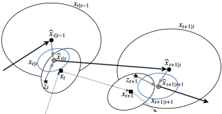
Figure 5. Pictorial representation of Kalman filtering.

6.3. Fusing partial observations of the state

In some problems, only a portion of the state can be measured directly. The observable portion of the state is specified formally using a full row-rank matrix $H_{t}$ called the observation matrix: if the state is x, what is observable is $H_{t}\textbf{\large{x}}$. For example, if the state vector has two components and only the first component is observable, $H_{t}$ can be $[\begin{smallmatrix}1&0\end{smallmatrix}]$. In general, the $H_{t}$ matrix can specify a linear relationship between the state and the observation, and it can be time-dependent. The imprecise measurement model introduced in Equation 36 becomes:

(37) $$\textbf{\large{z}}_{t}=H_{t}\textbf{\large{x}}_{t}+\textbf{\large{v}}_{t}$$

The hidden portion of the state can be specified using a matrix $C_{t}$, which is an orthogonal complement of $H_{t}$. For example, if $H_{t}=[\begin{smallmatrix}1&0\end{smallmatrix}]$, one choice for $C_{t}$ is $[\begin{smallmatrix}0&1\end{smallmatrix}]$.

Figure 4d shows the computation for this case. The fusion phase can be understood intuitively in terms of the following steps.

1. The observable part of the a priori estimate of the state $H_{t}\widehat{\textbf{\large{x}}}_{t|t-1}$ is fused with the measurement $\textbf{\large{z}}_{t}$, using the techniques developed in Sections 3-4. The quantity $\textbf{\large{z}}_{t}-H_{t}\widehat{\textbf{\large{x}}}_{t|t-1}$ is called the innovation. The result is the a posteriori estimate of the observable state $H_{t}\widehat{\textbf{\large{x}}}_{t|t}$.

2. The BLUE in Section 5 is used to obtain the a posteriori estimate of the hidden state $C_{t}\widehat{\textbf{\large{x}}}_{t|t}$ by adding to the a priori estimate of the hidden state $C_{t}\widehat{\textbf{\large{x}}}_{t|t-1}$ a value obtained from the product of the covariance between $H_{t}\textbf{\large{x}}_{t|t-1}$ and $C_{t}\textbf{\large{x}}_{t|t-1}$ and the difference between $H_{t}\widehat{\textbf{\large{x}}}_{t|t-1}$ and $H_{t}\widehat{\textbf{\large{x}}}_{t|t}$.

3. The a posteriori estimates of the observable and hidden portions of the state are composed to produce the a posteriori estimate of the entire state $\widehat{\textbf{\large{x}}}_{t|t}$.

The actual implementation produces the final result directly without going through these steps as shown in Figure 4d, but these incremental steps are useful for understanding how all this works, and they are implemented as follows.

1. The a priori estimate of the observable part of the state is $H_{t}\widehat{\textbf{\large{x}}}_{t|t-1}$ and the covariance is $H_{t}\Sigma_{t|t-1}H_{t}^{\rm T}$. The a posteriori estimate is obtained directly from Equation 31:

   $$H_{t}\widehat{\textbf{\large{x}}}_{t|t} =H_{t}\widehat{\textbf{\large{x}}}_{t|t-1}$$

   $$+H_{t}\Sigma_{t|t-1}H_{t}^{\rm T}(H_{t}\Sigma_{t|t-1}H_{t}^{\rm T}+R_{t})^{-1}(\textbf{\large{z}}_{t}-H_{t}\widehat{\textbf{\large{x}}}_{t|t-1})$$

   Let $K_{t}{=}\Sigma_{t|t-1}H_{t}^{\rm T}(H_{t}\Sigma_{t|t-1}H_{t}^{\rm T}+R_{t})^{-1}$. The a posteriori estimate of the observable state can be written in terms of $K_{t}$ as follows:

   (38) $$H_{t}\widehat{\textbf{\large{x}}}_{t|t} =H_{t}\widehat{\textbf{\large{x}}}_{t|t-1}+H_{t}K_{t}(\textbf{\large{z}}_{t}-H_{t}\widehat{\textbf{\large{x}}}_{t|t-1})$$

2. The a priori estimate of the hidden state is $C_{t}\widehat{\textbf{\large{x}}}_{t|t-1}$. The covariance between the hidden portion $C_{t}\textbf{\large{x}}_{t|t-1}$ and the observable portion $H_{t}\textbf{\large{x}}_{t|t-1}$ is $C_{t}\Sigma_{t|t-1}H_{t}^{\rm T}$. The difference between the a priori estimate and a posteriori estimate of $H_{t}\textbf{\large{x}}$ is $H_{t}K_{t}(\textbf{\large{z}}_{t}{-}H\widehat{\textbf{\large{x}}}_{t|t-1})$. Therefore the a posteriori estimate of the hidden portion of the state is obtained directly from Equation 33:

   $$C_{t}\widehat{\textbf{\large{x}}}_{t|t} =C_{t}\widehat{\textbf{\large{x}}}_{t|t-1}$$

   $$+(C_{t}\Sigma_{t|t-1}H_{t}^{\rm T})(H_{t}\Sigma_{t|t-1}H_{t}^{\rm T})^{-1}H_{t}K_{t}(\textbf{\large{z}}_{t}-H_{t}\widehat{\textbf{\large{x}}}_{t|t-1})$$

   (39) $$=C_{t}\widehat{\textbf{\large{x}}}_{t|t-1}+C_{t}K_{t}(\textbf{\large{z}}_{t}-H_{t}\widehat{\textbf{\large{x}}}_{t|t-1})$$

3. Putting the a posteriori estimates (38) and (39) together,

   $$\begin{pmatrix}H_{t}\\ C_{t}\end{pmatrix}\widehat{\textbf{\large{x}}}_{t|t} =\begin{pmatrix}H_{t}\\ C_{t}\end{pmatrix}\widehat{\textbf{\large{x}}}_{t|t-1}+\begin{pmatrix}H_{t}\\ C_{t}\end{pmatrix}K_{t}(\textbf{\large{z}}_{t}-H_{t}\widehat{\textbf{\large{x}}}_{t|t-1})$$

   Since $\begin{pmatrix}H_{t}\\ C_{t}\end{pmatrix}$ is invertible, it can be canceled from the left and right hand sides, giving the equation

   (40) $$\widehat{\textbf{\large{x}}}_{t|t} =\widehat{\textbf{\large{x}}}_{t|t-1}+K_{t}(\textbf{\large{z}}_{t}-H_{t}\widehat{\textbf{\large{x}}}_{t|t-1})$$

To compute $\Sigma_{t|t}$, Equation 40 can be rewritten as
$\widehat{\textbf{\large{x}}}_{t|t}=(I-K_{t}H_{t})\widehat{\textbf{\large{x}}}_{t|t-1}+K_{t}\textbf{\large{z}}_{t}$. Since $\textbf{\large{x}}_{t|t-1}$ and $\textbf{\large{z}}_{t}$ are uncorrelated, it follows from Lemma 2.2 that

$$\Sigma_{t|t}=(I-K_{t}H_{t})\Sigma_{t|t-1}(I-K_{t}H_{t})^{\rm T}+K_{t}R_{t}K_{t}^{\rm T}$$

Substituting the value of $K_{t}$ and simplifying, we get

(41) $$\Sigma_{t|t}=(I-K_{t}H_{t})\Sigma_{t|t-1}$$

Figure 4d puts all this together. In the literature, this dataflow is referred to as Kalman filtering. Unlike in Sections 3 and 4, the Kalman gain is not a dimensionless value here. If $H_{t}=I$, the computations in Figure 4d reduce to those of Figure 4c as expected.

Equation 40 shows that the a posteriori state estimate is a linear combination of the a priori state estimate ($\widehat{\textbf{\large{x}}}_{t|t-1}$) and the measurement ($\textbf{\large{z}}_{t}$). The optimality of this linear unbiased estimator is shown in the Appendix D. In Section 3.3, it was shown that incremental fusion of scalar estimates is optimal. The dataflow of Figures 4(c,d) computes the a posteriori state estimate at time $t$ by incrementally fusing measurements from the previous time steps, and this incremental fusion can be shown to be optimal using a similar argument.

6.4. Example: falling body

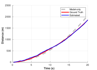
(a) Evolution of state: Distance

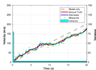
(b) Evolution of state: Velocity

Figure 6. Estimates of the object’s state over time.

To demonstrate the effectiveness of the Kalman filter, we consider an example in which an object falls from the origin at time $t{=}0$ with an initial speed of $0$ m/s and an expected constant acceleration of $9.8$ m/s² due to gravity. Note that acceleration in reality may not be constant due to factors such as wind, air friction, and so on.

The state vector of the object contains two components, one for the distance from the origin $s(t)$ and one for the velocity $v(t)$. We assume that only the velocity state can be measured at each time step. If time is discretized in steps of 0.25 seconds, the difference equation for the dynamics of the system is easily shown to be the following:

(42) $$\begin{pmatrix}v_{n}\\ s_{n}\end{pmatrix} =\begin{pmatrix}1&0\\ 0.25&1\end{pmatrix}\begin{pmatrix}v_{n-1}\\ s_{n-1}\end{pmatrix}+\begin{pmatrix}0&0.25\\ 0&0.5\times 0.25^{2}\end{pmatrix}\begin{pmatrix}0\\ 9.8\end{pmatrix}$$

where we assume $\begin{pmatrix}v_{0}\\ s_{0}\end{pmatrix}=\begin{pmatrix}0\\ 0\end{pmatrix}$ and $\Sigma_{0}={\begin{pmatrix}80&0\\ 0&10\end{pmatrix}}$.

The gray lines in Figure 6 show the evolution of velocity and distance with time according to this model. Because of uncertainty in modeling the system dynamics, the actual evolution of the velocity and position will be different in practice. The red lines in Figure 6 show one trajectory for this evolution, corresponding to a Gaussian noise term with covariance $\begin{pmatrix}2&2.5\\ 2.5&4\end{pmatrix}$ in Equation 34 (because this noise term is random, there are many trajectories for the evolution, and we are just showing one of them). The red lines correspond to “ground truth” in our example.

The green points in Figure 6b show the noisy measurements of velocity at different time steps, assuming the noise is modeled by a Gaussian with variance $8$. The blue lines show the a posteriori estimates of the velocity and position. It can be seen that the a posteriori estimates track the ground truth quite well even when the ideal system model (the gray lines) is inaccurate and the measurements are noisy. The cyan bars in the right figure show the variance of the velocity at different time steps. Although the initial variance is quite large, application of Kalman filtering is able to reduce it rapidly in few time steps.

6.5. Discussion

This section shows that Kalman filtering for state estimation in linear systems can be derived from two elementary ideas: optimal linear estimators for fusing uncorrelated estimates and best linear unbiased estimators for correlated variables. This is a different approach to the subject than the standard presentations in the literature. One standard approach is to use Bayesian inference. The other approach is to assume that the a posteriori state estimator is a linear combination of the form $A_{t}\widehat{\textbf{\large{x}}}_{t|t-1}{+}B_{t}\textbf{\large{z}}_{t}$, and then find the values of $A_{t}$ and $B_{t}$ that produce an unbiased estimator with minimum MSE. We believe that the advantage of the presentation given here is that it exposes the concepts and assumptions that underlie Kalman filtering.

Most presentations in the literature also begin by assuming that the noise terms $\textbf{\large{w}}_{t}$ in the state evolution equation and $\textbf{\large{v}}_{t}$ in the measurement are Gaussian. Some presentations (Babb, 2018; Faragher, 2012) use properties of Gaussians to derive the results in Sections 3 although as we have seen, these results do not depend on distributions being Gaussians. Gaussians however enter the picture in a deeper way if one considers nonlinear estimators. It can be shown that if the noise terms are not Gaussian, there may be nonlinear estimators whose MSE is lower than that of the linear estimator presented in Figure 4d. However if the noise is Gaussian, this linear estimator is as good as any unbiased nonlinear estimator (that is, the linear estimator is a minimum variance unbiased estimator (MVUE)). This result is proved using the Cramer-Rao lower bound (Rao, 1945).

7. Extension to nonlinear systems

The Extended Kalman Filter (EKF) and Unscented Kalman Filter (UKF) are heuristic approaches to using Kalman filtering for nonlinear systems. The state evolution and measurement equations for nonlinear systems with additive noise can be written as follows; in these equations, $f$ and $h$ are nonlinear functions.

(43) $$\textbf{\large{x}}_{t} =f(\textbf{\large{x}}_{t-1},\textbf{\large{u}}_{t})+\textbf{\large{w}}_{t}$$

(44) $$\textbf{\large{z}}_{t} =h(\textbf{\large{x}}_{t})+\textbf{\large{v}}_{t}$$

Intuitively, the EKF constructs linear approximations to the nonlinear functions $f$ and $h$ and applies the Kalman filter equations, while the UKF constructs approximations to probability distributions and propagates these through the nonlinear functions to construct approximations to the posterior distributions.

EKF

Examining Figure 4d, we see that the a priori state estimate in the predictor can be computed using the system model: $\widehat{\textbf{\large{x}}}_{t|t-1}=f(\widehat{\textbf{\large{x}}}_{t-1|t-1},\textbf{\large{u}}_{t})$. However, since the system dynamics and measurement equations are nonlinear, it is not clear how to compute the covariance matrices for the a priori estimate and the measurement. In the EKF, these matrices are computed by linearizing Equations 43 and 44 using the Taylor series expansions for the nonlinear functions $f$ and $h$. This requires computing the following Jacobians, which play the role of $F_{t}$ and $H_{t}$ in Figure 4d.

$$F_{t}=\frac{\partial f}{\partial\textbf{\large{x}}}\bigg{\rvert}_{\widehat{\textbf{\large{x}}}_{t-1|t-1},\textbf{\large{u}}_{t}}H_{t}=\frac{\partial h}{\partial\textbf{\large{x}}}\bigg{\rvert}_{\widehat{\textbf{\large{x}}}_{t|t-1}}$$

The EKF performs well in some applications such as navigation systems and GPS (Thrun et al., 2005).

UKF

When the system dynamics and observation models are highly nonlinear, the Unscented Kalman Filter (UKF) (Julier and Uhlmann, 2004) can be an improvement over the EKF. The UKF is based on the unscented transformation, which is a method for computing the statistics of a random variable x that undergoes a nonlinear transformation ($\textbf{\large{y}}=g(\textbf{\large{x}})$). The random variable x is sampled using a carefully chosen set of sigma points and these sample points are propagated through the nonlinear function $g$. The statistics of y are estimated using a weighted sample mean and covariance of the posterior sigma points. The UKF tends to be more robust and accurate than the EKF but has higher computation overhead due to the sampling process.

8. Conclusion

In this paper, we have shown that two concepts - optimal linear estimators for fusing uncorrelated estimates and best linear unbiased estimators for correlated variables - provide the underpinnings for Kalman filtering. By combining these ideas, standard results on Kalman filtering for linear systems can be derived in an intuitive and straightforward way that is simpler than other presentations of this material in the literature. This approach makes clear the assumptions that underlie the optimality results associated with Kalman filtering, and should make it easier to apply Kalman filtering to problems in computer systems.

Appendix A Basic probability theory and statistics terminology

Probability density function

For a continuous random variable $x$, a probability density function (pdf) is a function $p(x)$ whose value provides a relative likelihood that the value of the random variable will equal $x$. The integral of the pdf within a range of values is the probability that the random variable will take a value within that range.

If $g(x)$ is a function of $x$ with pdf $p(x)$, the expected value or expectation of $g(x)$ is $E[g(x)]$, defined as the following integral:

$$E[g(x)]=\int_{-\infty}^{\infty}g(x)p(x)dx$$

By definition, the mean $\mu_{x}$ of a random variable $x$ is $E[x]$. The variance of a random variable x measures the variability of the distribution. For the set of possible values of $x$, variance (denoted by $\sigma^{2}_{x}$) is defined by $\sigma^{2}_{x}=E[(x-\mu_{x})^{2}]$. The variance of a continuous random variable $x$ can be written as the following integral:

$$\sigma^{2}_{x}=\int_{-\infty}^{\infty}(x-\mu)^{2}p(x)dx$$

If $x$ is discrete and all outcomes are equally likely, then $\sigma^{2}_{x}=\frac{\Sigma(x_{i}-\mu_{x})^{2}}{n}$. The standard deviation $\sigma_{x}$ is the square root of the variance.

Covariance

The covariance of two random variables is a measure of their joint variability. The covariance between random variables $x_{1}:p_{1}{\sim}(\mu_{1},\sigma_{1}^{2})$ and $x_{2}:p_{2}{\sim}(\mu_{2},\sigma_{2}^{2})$ is the expectation $E[(x_{1}{-}\mu_{1}){*}(x_{2}{-}\mu_{2})]$. Two random variables are uncorrelated or not correlated if their covariance is zero. This is not the same concept as independence of random variables.

Two random variables are independent if knowing the value of one of the variables does not give us any information about the possible values of the other one. This is written formally as $p(x_{1}|x_{2})=p(x_{1})$; intuitively, knowing the value of $x_{2}$ does not change the probability that $p_{1}$ takes a particular value.

Independent random variables are uncorrelated but random variables can be uncorrelated even if they are not independent. It can be shown that if $x_{1}$ and $x_{2}$ are not correlated, $E[x_{1}|x_{2}]{=}E[x_{1}]$; intuitively, knowing the value of $x_{2}$ may change the probability that $x_{1}$ takes a particular value, but the mean of the resulting distribution remains the same as the mean of $x_{1}$. A special case of this that is easy to understand are examples in which knowing $x_{2}$ restricts the possible values of $x_{1}$ without changing the mean. Consider a random variable $u:U$ that is uniformly distributed over the unit circle, and consider random variables $x_{1}:[-1,1]$ and $x_{2}:[-1,1]$ that are the projections of $u$ on the $x$ and $y$ axes respectively. Given a value for $x_{2}$, there are only two possible values for $x_{1}$, so $x_{1}$ and $x_{2}$ are not independent. However, the mean of these values is 0, which is the mean of $x_{1}$, so $x_{1}$ and $x_{2}$ are not correlated.

Appendix B Matrix Derivatives

If $f({X})$ is a scalar function of a matrix ${X}$, the matrix derivative $\frac{\partial f({X})}{\partial{X}}$ is defined as the matrix

$\left(\begin{array}[]{ccc}\frac{\partial f({X})}{\partial X(1,1)}&...&\frac{\partial f({X})}{\partial X(1,n)}\\ ...&...&...\\ \frac{\partial f({X})}{\partial X(n,1)}&...&\frac{\partial f({X})}{\partial X(n,n)}\end{array}\right)$

Lemma B.1.

Let X be a $m\times n$ matrix, a be a $m\times 1$ vector, b be a $n\times 1$ vector.

(45) $$\frac{\partial\textbf{\large{a}}^{T}{X}\textbf{\large{b}}}{\partial{X}} =\textbf{\large{a}}\textbf{\large{b}}^{T}$$

(46) $$\frac{\partial(\textbf{\large{a}}^{T}{X}^{T}{X}\textbf{\large{b}})}{\partial{X}} ={X}(\textbf{\large{a}}\textbf{\large{b}}^{T}+\textbf{\large{b}}\textbf{\large{a}}^{T})$$

(47) $$\frac{\partial(trace(XBX^{T}))}{\partial X} =XB^{T}+XB$$

See Petersen and Pedersen for a proof (Petersen and Pedersen, 2012).

Appendix C Proof of Theorem 4.1

Theorem 4.1, which is reproduced below for convenience, can be proved using matrix derivatives.

Theorem 0.

Let pairwise uncorrelated estimates $\textbf{\large{x}}_{i}(1{\leq}i{\leq}n)$ drawn from distributions $p_{i}(x){=}(\boldsymbol{\mu}_{i},{\Sigma}_{i})$ be fused using the linear model $\textbf{\large{y}}_{A}(\textbf{\large{x}}_{1},..,\textbf{\large{x}}_{n})=\sum_{i=1}^{n}{A}_{i}\textbf{\large{x}}_{i}$, where $\sum_{i=1}^{n}{A}_{i}={I}$. The $MSE(\textbf{\large{y}}_{A})$ is minimized for

$${A}_{i} =(\smashoperator[r]{\sum_{{\rm j}=1}^{n}}{\Sigma}_{j}^{-1})^{-1}{\Sigma}_{i}^{-1}.$$

Proof.

To use the Lagrange multiplier approach, we can convert the constraint $\sum_{i=1}^{n}{A}_{i}={I}$ into a set of $m^{2}$ scalar equations (for example, the first equation would be $A_{1}(1,1)+A_{2}(1,1)+..+A_{n}(1,1)=1$), and then introduce $m^{2}$ Lagrange multipliers, which can denoted by $\lambda(1,1),...\lambda(m,m)$.

This obscures the matrix structure of the problem so it is better to implement this idea implicitly. Let ${\Lambda}$ be an $m{\times}m$ matrix in which each entry is one of the scalar Lagrange multipliers we would have introduced in the approach described above. Analogous to the inner product of vectors, we can define the inner product of two matrices as ${<}A,B{>}=trace(A^{\rm T}B)$ (it is easy to see that ${<}A,B{>}$ is $\sum_{i=1}^{m}\sum_{j=1}^{m}A(i,j)B(i,j)$). Using this notation, we can formulate the optimization problem using Lagrange multipliers as follows:

$$f({A}_{1},...,{A}_{n})=E\big{\{}\smashoperator[r]{\sum_{i=1}^{n}}(\textbf{\large{x}}_{i}-\boldsymbol{\mu}_{i})^{\rm T} {{A}_{i}}^{\rm T}{A}_{i}(\textbf{\large{x}}_{i}-\boldsymbol{\mu}_{i})\big{\}}$$

$$+\big{<}{\Lambda},\big{(}\smashoperator[r]{\sum_{i=1}^{n}}{A}_{i}-{I}\big{)}\big{>}$$

Taking the matrix derivative of $f$ with respect to each A_i and setting each derivative to zero to find the optimal values of $A_{i}$ gives us the equation $E\big{\{}2{A}_{i}(\textbf{\large{x}}_{i}-\boldsymbol{\mu}_{i})(\textbf{\large{x}}_{i}-\boldsymbol{\mu}_{i})^{\rm T}+{\Lambda}\big{\}}=0$.

This equation can be written as $2{A}_{i}{\Sigma}_{i}+{\Lambda}=0$, which implies

$${A}_{1}{\Sigma}_{1}={A}_{2}{\Sigma}_{2}=...={A}_{n}{\Sigma}_{n}=-\frac{{\Lambda}}{2}$$

Using the constraint that the sum of all A_i equals to the identity matrix ${I}$ gives us the desired expression for ${A}_{i}$:

$${A}_{i} =(\smashoperator[r]{\sum_{{\rm j}=1}^{n}}{\Sigma}_{j}^{-1})^{-1}{\Sigma}_{i}^{-1}$$

∎

Appendix D Proof of the Optimality of Equation 40

We show that ($\widehat{\textbf{\large{x}}}_{t|t}=\widehat{\textbf{\large{x}}}_{t|t-1}+K_{t}(\textbf{\large{z}}_{t}-H_{t}\widehat{\textbf{\large{x}}}_{t|t-1})$) (Equation 40) is an optimal unbiased linear estimator for fusing the a priori state estimate with the measurement at each step. The proof has two steps: we show that this estimator is unbiased, and then show it is optimal.

Unbiased condition:

We prove a more general result that characterizes unbiased linear estimators for this problem, assuming that the prediction stage (Figure 4(d)) is unchanged. The general form of the linear estimator for computing the a posteriori state estimate is

(48) $$\widehat{\textbf{\large{y}}}_{t|t}=A_{t}*\widehat{\textbf{\large{y}}}_{t|t-1}+B_{t}*\textbf{\large{z}}_{t}$$

It is unbiased if $E[\widehat{\textbf{\large{y}}}_{t|t}]{=}E[\textbf{\large{x}}_{t}]$, and we show that this is true if $A_{t}{=}{(}I{-}B_{t}{)}*H_{t}$.

The proof is by induction on $t$. By assumption, $E[\widehat{\textbf{\large{y}}}_{0|0}]=E[\textbf{\large{x}}_{0}]$. Assume inductively that $E[\widehat{\textbf{\large{y}}}_{t{-}1|t{-}1}]{=}E[\textbf{\large{x}}_{t{-}1}]$.

(a) We first prove that the predictor is unbiased.

$$\widehat{\textbf{\large{y}}}_{t|t{-}1} ={F}_{t}{*}\widehat{\textbf{\large{y}}}_{t{-}1|t{-}1}+{B}_{t}{*}\textbf{\large{u}}_{t}\text{\ \ (Predictor in Figure~{}\ref{fig:dynamics})}$$

$$E[\widehat{\textbf{\large{y}}}_{t|t-1}] ={F}_{t}*E[\widehat{\textbf{\large{y}}}_{t{-}1|t{-}1}]+{B}_{t}{*}\textbf{\large{u}}_{t}$$

$$={F}_{t}*E[\textbf{\large{x}}_{t-1}]+{B}_{t}{*}\textbf{\large{u}}_{t}\text{\ \ (By inductive assumption)}$$

$$=E[{F}_{t}*\textbf{\large{x}}_{t-1}+{B}_{t}{*}\textbf{\large{u}}_{t}]$$

$$=E[{F}_{t}*\textbf{\large{x}}_{t-1}+{B}_{t}{*}\textbf{\large{u}}_{t}+\textbf{\large{w}}_{t}]\ \ \text{($\textbf{\large{w}}_{t}$ is zero mean)}$$

$$=E[\textbf{\large{x}}_{t}]\text{\ \ (From state evolution equation~{}\ref{eqn:state_evolution})}$$

(b) We prove that the estimator in Equation 48 is unbiased if $A_{t}{=}{(}I{-}B_{t}{)}*H_{t}$.

$$E[\widehat{\textbf{\large{y}}}_{t|t}] =E[A_{t}*\widehat{\textbf{\large{y}}}_{t|t-1}+B_{t}*\textbf{\large{z}}_{t}]\ \ \text{(From Equation~{}\ref{eqn:kfGeneral})}$$

$$=A_{t}*E[\widehat{\textbf{\large{y}}}_{t|t-1}]+B_{t}*E[\textbf{\large{z}}_{t}]$$

$$=A_{t}*E[\textbf{\large{x}}_{t}]+B_{t}*E[H_{t}\textbf{\large{x}}_{t}+\textbf{\large{v}}_{t}]\ \ \text{(Equation~{}\ref{eqn:observation_eqn_H} for $\textbf{\large{z}}_{t}$)}$$

$$=A_{t}*E[\textbf{\large{x}}_{t}]+B_{t}*H_{t}*E[\textbf{\large{x}}_{t}]\ \ \text{(Because $\textbf{\large{v}}_{t}$ is zero mean)}$$

$$=(A_{t}+B_{t}*H_{t})*E[\textbf{\large{x}}_{t}]$$

The estimator is unbiased if $(A_{t}+B_{t}*H_{t})=I$, which is equivalent to requiring that $A_{t}=(I-B_{t}*H_{t})$. Therefore the general unbiased linear estimator is of the form

$$\widehat{\textbf{\large{y}}}_{t|t} =(I-B_{t}*H_{t})*\widehat{\textbf{\large{y}}}_{t|t-1}+B_{t}*\textbf{\large{z}}_{t}$$

(49) $$=\widehat{\textbf{\large{y}}}_{t|t-1}+B_{t}*(\textbf{\large{z}}_{t}-H_{t}*\widehat{\textbf{\large{y}}}_{t|t-1})$$

Since Equation 40 is of this form, it is an unbiased linear estimator.

Optimality:

We now show that using $B_{t}=K_{t}$ at each step is optimal, assuming that this is done at all time steps before $t$. Since $\textbf{\large{z}}_{t}$ and $\textbf{\large{y}}_{t|t-1}$ are uncorrelated, we can use Lemma 2.2 to compute the covariance matrix of $\widehat{\textbf{\large{y}}}_{t|t}$, denoted by $\Xi_{t|t}$. This gives $\Xi_{t|t}=(I-B_{t}H_{t})\Sigma_{t|t-1}(I-B_{t}H_{t})^{\rm T}+B_{t}R_{t}B_{t}^{\rm T}$. The $MSE$ is the trace of this matrix, and we need to find $B_{t}$ that minimizes this trace. Using matrix derivatives (Equation 47), we see that

$$\frac{\partial(trace(\Xi_{t|t}))}{\partial B_{t}}=-2(I-B_{t}H_{t})\Sigma_{t|t-1}H_{t}^{T}+2*B_{t}R_{t}$$

Setting this zero and solving for $B_{t}$ gives
$B_{t}=\Sigma_{t|t-1}H_{t}^{T}[H_{t}\Sigma_{t|t-1}H_{t}^{T}+R_{t}]^{-1}$. This is exactly $K_{t}$, proving that Equation 40 is an optimal unbiased linear estimator.

Comment:

This proof of optimality provides another way of deriving Equation 40. We believe the constructive approach described in Section 6 provides more insight into how and why Kalman filtering works. The ideas in that construction can be used to provide a different proof of optimality.