Using modular decomposition technique to solve the maximum clique problem

Abstract

In this article we use the modular decomposition technique for exact solving the weighted maximum clique problem. Our algorithm takes the modular decomposition tree from the paper of Tedder et. al. and finds solution recursively. Also, we propose algorithms to construct graphs with modules. We show some interesting results, comparing our solution with Ostergard’s algorithm on DIMACS benchmarks and on generated graphs

1 Introduction

Today graphs can be used in variety fields, such as biology, chemistrybib1 ; bib4 , data analysis, mathematics and others, as a structure of data. Due to enormous expand of information, the size of graphs for analysis is increasing, it can be hundred, thousand and even hundred of thousands vertices. Since the computational time of any algorithm on graphs depends on its size, it has become a great problem for community. There are many graph decomposition techniques to reduce a graph to its smaller fragments; one of them is modular decomposition. In this article we use the fastest algorithm for constructing modular decomposition proposed by Tedder et. albib2 . It creates a modular decomposition tree for any input graphs in linear time. Then we use this tree to solve the maximum clique problem on graphs from DIMACS benchmarks using Ostergard’sbib5 algorithm, and compare computational time with Ostergard’s algorithm without modular decomposition technique. Also, we construct some other types of graphs, such as co-graphs and graphs of mutual simplicity.

2 Modular decomposition algorithm

Module $M$ of graph $G(V,E)$ is a subset of vertices, where all of them have the same neighbors outside the set. For example, on the figure 1 vertices $a,b,c$ is a module, because each has one common neighbor vertex $d$. Also vertices $f$ and $e$ construct a module with common neighbors $d$ and $g$. As it seen from example, inside module vertices can be connected and/or disconnected. It results in three types of modules: parallel, series and prime. The first one describes module, where all of his vertices are disconnected, so it is basically an independent set. Whereas the second one is characterized by connected vertices. Finally, the third one relates to the set in which not all vertices are connected.
The modular decomposition technique suggest reducing module to one vertex with some changed quality, for example it can be weight, label or color depends on problem, and after finding all modules and reducing them, we get graph with less vertices.
So first, we take module $a,b,c$ and make one vertex $abc$ figure 2, than reduce module $e,f$ to vertex $ef$. As result the input graph has $4$ vertices figure 3.

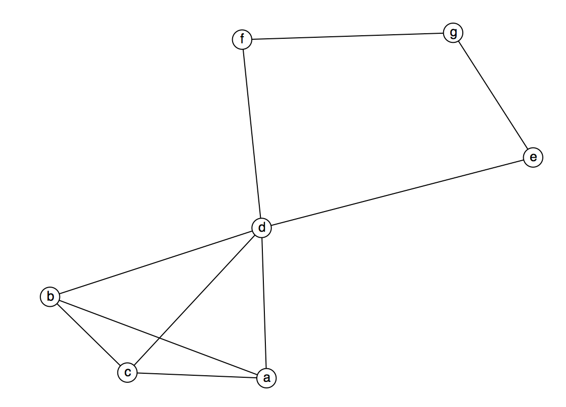
Figure 1: Example 1bib6

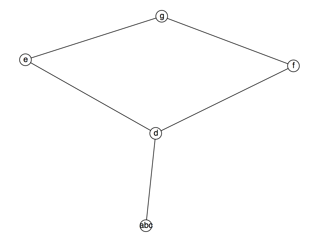
Figure 2: Step 1 of reducing graph sizebib6

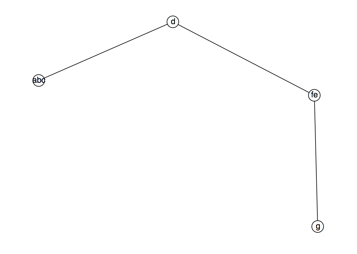
Figure 3: Step 2 of reducing graph sizebib6

Tedder et. al. proposed a linear algorithm for constructing modular decomposition tree in which the root represents input graph, its children represent strong modules (modules which do not overlap each other), after that each model decomposes to its strong module and so on, leaves of this tree are vertices of the input graph. An example of such tree shown on Diagram 1.

[.Prime [.Series [.a ] [.b ] [.c ]] [.d ] [.Parallel [.e ] [.f ]] [.g ]]

List of diagrams 1 Example of MD tree for graph from example 1

3 Maximum clique problem

Clique $C$ of a graph $G(V,C)$ is a subset of vertices which all of them are connected to each other.
Maximum clique (MC) is a clique which has a maximum size or weight, if there are weights to vertices.
MC problem is the NP-hard problem so why increasing the size of the input graph leads us to increasing computational time of any exact solver exponentially.

4 The maximum clique solver based on the modular decomposition tree

Our algorithm takes the modular decomposition tree as input data and recursively as depth-first search compute maximum clique on each level, as it solves all its children. See the pseudo code:

function $solve$($node$)

     if $node$ $is$ $leave$ then

         return $this$ $node$ $with$ $it^{\prime}s$ $weight$

     end if

     if $node$ $has$ $type$ $parallel$ then

         return $max(solve(children))$

     end if

     if $node$ $has$ $type$ $series$ then

         return $sum(solve(children))$

     end if

     if $node$ $has$ $type$ $prime$ then

         $subgraph=create-subgraph(children)$

         return $Ostergard(subgraph)$

     end if

end function

There are tree types of nodes: parallel, series and prime. When it finds node with the parallel type, it returns max of solution for its children, because they are not connected and cannot become a clique. When it finds nodes with the series type, it returns sum of children, as they are all connected. If the node $i$ type is prime algorithm constructs a new graph, which has $n_{i}$ vertices ($n_{i}$ - the number of modules for node $i$), connects them as in input graph and gives them weights as results of calculation of MC problem and then solve it using some general algorithm for weighted maximum clique problem. In our case we use Ostergard’s algorithm, because it easily implements in our algorithm, due to input data.
Our approach was to create such algorithm and compare it with some known solver, like Ostergard. In this article we show results against Ostergard, because it was used inside suggested approach.
Let’s consider the graph in figure 1 and its modular decomposition tree from diagram 1. Our algorithm goes to leaf $a$ and rerurns $1$, because there is no weight to vertices, also from leafs $b$ and $c$ it returns $1$, then the algorithm goes to the node with the type series and returns $3$ as sum of $1$, $1$, $1$. At leaf $d$ and $g$ it returns $1$. At the parallel node it returns also $1$, because node $e$ and node $f$ have the same weight, if they have different weight, it will return maximum. After that at the node with type prime it constructs graph with $4$ vertices with weight $3$, $1$, $1$ and $1$ and the structure as at the figure 3, use solver and gets a solution maximum clique $a,b,c,d$ with weight is equal $4$.

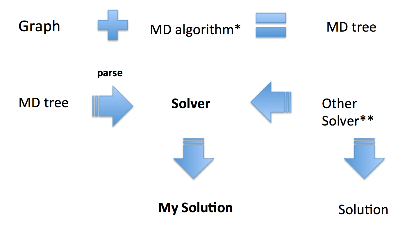
Figure 4: Structure of algorithm
*Marc Tedder. Derek Corneil. Michel Habib. and Christophe Paul ”Simpler Linear-Time Modular Decomposition via Recursive Factorizing Permutations”
** Patric R. J. Ostergard

5 Results on DIMACS benchmarks

After using the algorithm of Tedder et al on DIMACS benchmarks, it was found that only few of graphs has modules, so we compare results only with them. See table 1.

Size	My algorithm (s)	MD (s)	My + MD (s)	Ostergard (s)
c-fat200-1	0.000118	0.068662612	0.068780612	0.001059
c-fat200-2	0	0.104443933	0.104443933	0.001371
c-fat200-5	0	0.226667621	0.226667621	2.61894
c-fat500-1	0.015956	0.147924545	0.163880545	0.002184
c-fat500-10	0.006224	0.680824483	0.687048483	0.011369
c-fat500-2	0.011647	0.216331646	0.227978646	0.003734
c-fat500-5	0.009128	0.324011131	0.333139131	0.006868

Table 1: Results on DIMACS benchmarks

As can be seen from the result table our algorithm is faster only on $c-fat200-5$, and after analysis of MD tree of this graphs, we found, that for this particular graph MD tree contains only parallel and series types of nodes. So we thought that we can create such structures to test on them.

6 Algorithms for generation graphs with modules

In this article there are two proposed algorithms to generate graphs, which in their MD tree contains only parallel and series types of nodes. It helps us to find a solution on each node easily.

6.1 Graphs of mutual simplicity

Graph of mutual simplicity generate as follows, we connect two vertices $i$ and $j$ only if their greatest common divisor equals to $1$, for example see 5.

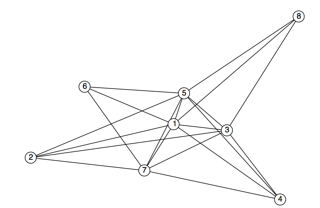
Figure 5: Graph of mutual simplicity with 8 nodes

For this graph you can see MD tree on Diagram 2.

[.Series [.7 ] [.1 ] [.Parallel [.6 ] [.Series [.3 ] [.Parallel [.8 ] [.4 ] [.Series [.2 ] [.5 ] ] ] ] ] ]

List of diagrams 2 MD tree for graph of mutual simplicity with 8 vertices

6.2 Co-Graphs

In this case we try to build MD tree by recursively partition giving nodes to modules and randomly assign its type as parallel or series. The algorithm works as follows:

function $partition$($n$)

     $parts=[]$

     while $n>0$ do

         $p=randind(1,n)$

         $parts.append(p)$

         $n=n-p$

     end while

     return $parts$

end function

function $CreateCoGraph$($n$)

     if $n>1$ then

         $parts=reverse(partition(n))$

         if $randint(0,1)==0$ then

              $graph$

              for $partinparts$ do

                  $subgraph=createCo-Graphs(part)$

                  $graph.add(subgraph)$

              end for

         else

              $graph$

              for $partinparts$ do

                  $subgraph=createCo-Graphs(part)$

                  $graph.add(subgraph)$

              end for

              $connect$ $all$ $subgraph$

         end if

         return $graph$

     end if

end function

7 Results on generated graphs

7.1 Graphs of mutual simplicity

Size	My algorithm(s)	MD(s)	My+MD(s)	Ostergard(s)
100	0	0.06906381	0.06906	0.001743
150	0	0.160086907	0.16009	0.004758
200	0	0.311571475	0.31157	0.006921
1000	0.00015	0.830395642	0.83055	300.001
1050	0.000132	2.77094437	2.77108	0.709009
1100	0.000149	2.962479483	2.96263	300
1150	0.00014	1.005088013	1.00523	300
1200	0.000178	1.102902136	1.10308	300
1250	0.000163	3.624508829	3.62467	300
1300	0.000237	6.191885617	6.19212	300
1350	0.000169	3.158776487	3.15895	300
1400	0.000192	0.448514811	0.44871	300
1450	0.000263	5.838179619	5.83844	300
1500	0.000273	8.211194675	8.21147	300
1550	0.000358	1.049262402	1.04962	300
1600	0.000262	1.861131225	1.86139	300
1650	0.000268	2.108732494	2.10900	300
1700	0.000283	13.137433843	13.13772	300
1750	0.000284	6.082156016	6.08244	300
1800	0.000295	2.649852882	2.65015	300
1850	0.00024	1.641608819	1.64185	300
1900	0.000331	22.834692949	22.83502	300
1950	0.000284	15.864648365	15.86493	300
2050	0.000315	19.971808447	19.97212	300
2100	0.000323	6.728151243	6.72847	300
2200	0.000331	3.152012792	3.15234	300
2250	0.000347	3.20890262	3.20925	300
2300	0.000519	26.991591521	26.99211	300
2350	0.000395	26.367774638	26.36817	300
2400	0.000368	17.514787453	17.51516	300
2450	0.00046	41.651295783	41.65176	300

Table 2: Results on graphs mutual simplicity

7.2 Co-Graphs

Size	My algorithm(s)	MD(s)	My+MD(s)	Ostergard(s)
500	107 vertices 0.000119	0.599508522	0.599627522	107 vertices 5.19397
550	219 vertices 0.000128	1.126792247	1.126920247	219 vertices 0.420204
600	206 vertices 0.000123	1.613567235	1.613690235	206 vertices 0.385463
650	143 vertices 0.000124	1.079984486	1.080108486	37 vertices 300
700	197 vertices 0.000151	1.49792208	1.49807308	197 vertices 0.10201
750	279 vertices 0.000184	2.111751452	2.111935452	279 vertices 0.096327
800	92 vertices 0.00017	0.592107428	0.592277428	37 vertices 300
850	155 vertices 0.000172	1.634152987	1.634324987	29 vertices 300
900	134 vertices 0.00016	1.25222059	1.25238059	36 vertices 300
1000	241 vertices 0.00018	3.105684402	3.105864402	241 vertices 4.2414
1050	338 vertices 0.000162	4.151108273	4.151270273	116 vertices 300
1100	329 vertices 0.000182	4.811745176	4.811927176	329 vertices 19.4748
1150	408 vertices 0.000139	5.756633889	5.756772889	408 vertices 0.302615
1200	362 vertices 0.000165	5.614880477	5.615045477	362 vertices 2.85711
1250	151 vertices 0.000193	2.125359674	2.125552674	54 vertices 300
1300	292 vertices 0.00019	5.384282824	5.384472824	292 vertices 12.8855
1350	178 vertices 0.000214	2.035435868	2.035649868	63 vertices 300
1400	216 vertices 0.000186	2.634297357	2.634483357	32 vertices 300
1450	279 vertices 0.00026	5.657872455	5.658132455	35 vertices 300
1500	377 vertices 0.000217	9.239033114	9.239250114	377 vertices 13.7176
1550	238 vertices 0.000268	6.540190934	6.540458934	238 vertices 19.8803
1600	409 vertices 0.000262	10.753900639	10.75416264	409 vertices 48.6752
1650	278 vertices 0.00028	10.456971305	10.45725131	41 vertices 300
1700	229 vertices 0.000327	10.474212124	10.47453912	30 vertices 300
1800	543 vertices 0.000345	21.152246751	21.15259175	47 vertices 300
1850	494 vertices 0.000296	18.978203233	18.97849923	43 vertices 300
1900	263 vertices 0.000303	5.338127994	5.338430994	103 vertices 300
1950	355 vertices 0.000308	17.914419038	17.91472704	44 vertices 300

Table 3: Results on Co-Graphs

8 Conclusion

As can be seen from the result our algorithm works faster on graphs without prime nodes in the MD tree. It happens due to necessity to construct a subgraph and call different solver for it to calculate the maximum clique at this step. Also you can notice that the construct of MD tree takes the significant amount of calculation time, though algorithm is linear.

Funding

This article is partially supportеd by LATNA laboratory, National Research University Higher School of Economics.

References

- (1) Gagneur, J., Krause, R., Bouwmeester,T. & Casari, G. Modular decompositionof protein-protein interaction networks.Genome Biol 5, R57 (2004)
- (2) Habib M., Paul C., A survey on algorithmic aspects of modular decomposition, Computer Science Review, 4: 41–59 (2010)
- (3) Kuhl F. S., Crippen G. M., Friesen, D. K., A combinatorial algorithm for calculating ligand binding, Journal of Computational Chemistry,5 (1): 24-–34 (1983)
- (4) Patric R.J.Östergård, A fast algorithm for the maximum clique problem, Discrete Applied Mathematics, Volume 120, Issues 1–-3, Pages 197–207(2002)
- (5) Rhodes Nicholas, Willett Peter, Calvet Alain, Dunbar James B., Humblet Christine, CLIP: similarity searching of 3D databases using clique detection, Journal of Chemical Information and Computer Sciences, 43 (2): 443–-448 (2003)
- (6) Tedder M., Corneil D. , Habib M., Paul C. ,Simpler linear-time modular decomposition via recursive factorizing permutations, 35th International Colloquium on Automata, Languages and Programming, ICALP2008, Part 1, LNCS, vol. 5125, Springer, 634–64 (2008)