language=bash,basicstyle=,breaklines=true,identifierstyle=,stringstyle=,commentstyle=,showstringspaces=false,emph=[1]$,emphstyle=[1], emph=[2]cd, git, clone, checkout, pull, fetch, commit, rebase, emphstyle=[2],

Creation and analysis of biochemical constraint-based models: the COBRA Toolbox v3.0

11th March 2024

Laurent Heirendt¹ & Sylvain Arreckx¹, Thomas Pfau², Sebastián N. Mendoza^3,18, Anne Richelle⁴, Almut Heinken¹, Hulda S. Haraldsdóttir¹, Jacek Wachowiak¹, Sarah M. Keating⁵, Vanja Vlasov¹, Stefania Magnusdóttir¹, Chiam Yu Ng⁶, German Preciat¹, Alise Žagare¹, Siu H.J. Chan⁶, Maike K. Aurich¹, Catherine M. Clancy¹, Jennifer Modamio¹, John T. Sauls⁷, Alberto Noronha¹, Aarash Bordbar⁸, Benjamin Cousins⁹, Diana C. El Assal¹, Luis V. Valcarcel¹⁰, Iñigo Apaolaza¹⁰, Susan Ghaderi¹, Masoud Ahookhosh¹, Marouen Ben Guebila¹, Andrejs Kostromins¹¹, Nicolas Sompairac²², Hoai M. Le¹, Ding Ma¹², Yuekai Sun¹², Lin Wang⁶, James T. Yurkovich¹³, Miguel A.P. Oliveira¹, Phan T. Vuong¹, Lemmer P. El Assal¹, Inna Kuperstein²², Andrei Zinovyev²², H. Scott Hinton¹⁴, William A. Bryant¹⁵, Francisco J. Aragón Artacho¹⁶, Francisco J. Planes¹⁰, Egils Stalidzans¹¹, Alejandro Maass^3,18, Santosh Vempala⁹, Michael Hucka¹⁷, Michael A. Saunders¹², Costas D. Maranas⁶, Nathan E. Lewis^4,19, Thomas Sauter², Bernhard Ø. Palsson^13,21, Ines Thiele¹, Ronan M.T. Fleming¹

This protocol is an update to Nature Protocols 2(3), 727–738, March (2007); doi:10.1038/nprot.2007.99; published online 29 March 2007 and Nature Protocols 6 (9), 1290-1307 (2011); doi:10.1038/protex.2011.234; published online 11 May 2011.

Abstract

COnstraint-Based Reconstruction and Analysis (COBRA) provides a molecular mechanistic framework for integrative analysis of experimental data and quantitative prediction of physicochemically and biochemically feasible phenotypic states. The COBRA Toolbox is a comprehensive software suite of interoperable COBRA methods. It has found widespread applications in biology, biomedicine, and biotechnology because its functions can be flexibly combined to implement tailored COBRA protocols for any biochemical network. Version 3.0 includes new methods for quality controlled reconstruction, modelling, topological analysis, strain and experimental design, network visualisation as well as network integration of chemoinformatic, metabolomic, transcriptomic, proteomic, and thermochemical data. New multi-lingual code integration also enables an expansion in COBRA application scope via high-precision, high-performance, and nonlinear numerical optimisation solvers for multi-scale, multi-cellular and reaction kinetic modelling, respectively. This protocol can be adapted for the generation and analysis of a constraint-based model in a wide variety of molecular systems biology scenarios. This protocol is an update to the COBRA Toolbox 1.0 and 2.0. The COBRA Toolbox 3.0 provides an unparalleled depth of constraint-based reconstruction and analysis methods.

Metabolic models, metabolic reconstruction, metabolic engineering, gap filling, strain engineering, omics, data integration, metabolomics, transcriptomics, constraint-based modelling, computational biology, bioinformatics, biochemistry, human metabolism, and microbiome analysis.

¹Luxembourg Centre for Systems Biomedicine, University of Luxembourg, 6 avenue du Swing, Belvaux, L-4367, Luxembourg.

²Life Sciences Research Unit, University of Luxembourg, 6 avenue du Swing, Belvaux, L-4367, Luxembourg.

³Center for Genome Regulation (Fondap 15090007), University of Chile, Blanco Encalada 2085, Santiago, Chile.

⁴Department of Pediatrics, University of California, San Diego, School of Medicine, La Jolla, CA 92093, USA.

⁵European Molecular Biology Laboratory, European Bioinformatics Institute (EMBL-EBI), Hinxton, Cambridge, CB10 1SD, United Kingdom.

⁶Department of Chemical Engineering, The Pennsylvania State University, University, University Park, PA 16802, USA.

⁷Department of Physics, University of California, San Diego, 9500 Gilman Dr., La Jolla, CA 92093, USA; Bioinformatics and Systems Biology Program, University of California, San Diego, La Jolla, CA, USA.

⁸Sinopia Biosciences, San Diego, CA, USA.

⁹School of Computer Science, Algorithms and Randomness Center, Georgia Institute of Technology, Atlanta, GA, USA.

¹⁰Biomedical Engineering and Sciences Department, TECNUN, University of Navarra, Paseo de Manuel Lardizabal, 13, 20018, San Sebastian, Spain.

¹¹Institute of Microbiology and Biotechnology, University of Latvia, Jelgavas iela 1, Riga LV-1004, Latvia.

¹²Department of Management Science and Engineering, Stanford University, Stanford CA 94305-4026, USA.

¹³Bioengineering Department, University of California, San Diego, La Jolla, CA, USA.

¹⁴Utah State University Research Foundation, 1695 North Research Park Way, North Logan, Utah 84341, USA.

¹⁵Centre for Integrative Systems Biology and Bioinformatics, Department of Life Sciences, Imperial College London, London, United Kingdom.

¹⁶Department of Mathematics, University of Alicante, Spain.

¹⁷California Institute of Technology, Computing and Mathematical Sciences, MC 305-16, 1200 E. California Blvd., Pasadena, CA 91125, USA.

¹⁸Mathomics, Center for Mathematical Modeling, University of Chile, Beauchef 851, 7th Floor, Santiago, Chile.

¹⁹Novo Nordisk Foundation Center for Biosustainability at the University of California, San Diego, La Jolla, CA 92093, United States.

²⁰Latvian Biomedical Research and Study Centre, Ratsupites iela 1, Riga, LV1067, Latvia.

²¹Novo Nordisk Foundation Center for Biosustainability, Technical University of Denmark, Kemitorvet, Building 220, 2800 Kgs. Lyngby, Denmark.

²²Institut Curie, PSL Research University, Mines Paris Tech, Inserm, U900, F-75005, Paris, France.

Correspondence should be addressed to Ronan M.T. Fleming (ronan.mt.fleming@gmail.com).

INTRODUCTION

Development of the protocol

In the past two decades, significant developments in molecular biology have led to a deluge of data on the molecular composition of organisms and their environment. Quantitative molecular measurements at genome scale are now routine and include genomic, metabolomic, transcriptomic, and proteomic data. This wealth of data has stimulated the development of a wide variety of algorithms and software for data preprocessing and analysis. Preprocessing converts the measured variables into estimates of the quantity of each molecular species present in a sample. Analysis takes this quantification of molecular species to derive new biological knowledge. Despite many advances and novel discoveries, it remains a major challenge for the biology community to be able to derive insight from experiments in a way that leads to a deeper understanding of a biological system.

Analysis techniques may be split into those that do and those that do not incorporate prior information on a system in question. All else being equal, an integrative analysis technique that incorporates prior information from complementary experiments will typically outperform a technique that does not, because corroboration with data from complementary experimental platforms can be used to increase the confidence that an observation is real. Fundamentally, integrative analysis is successful because it is an expression of a Bayesian statistical approach whereby prior information from complementary experiments represents the knowledge about a system before a new experiment. Thus, integrative analysis is an inference procedure to update the knowledge about the system in light of new data from an additional experiment.

Integrative analysis can be either mechanistic or non-mechanistic. Mechanistic techniques rely on using molecular mechanistic models to represent prior information on the biochemical networks underlying the data being analysed. Non-mechanistic integrative analysis is often used to study ’omics’ data and is essential when nothing is known about the underlying molecular mechanisms. However, often a subset of the underlying molecular mechanisms is known. Thus, a significant limitation of non-mechanistic integrative analysis is that it ignores the decades of prior information from molecular mechanistic experimental studies in biochemistry, molecular biology, etc. As such, non-mechanistic integrative analysis omits valuable prior information from its biochemical network context and from the general physicochemical principles that any biochemical network must obey.

A genome-scale metabolic reconstruction (see Figure 1) is a structured knowledge-base that abstracts pertinent information on the biochemical transformations taking place within a chosen biochemical system, e.g., the human gut microbiome[1]. Constraint-based reconstruction and analysis (COBRA[2]) is a mechanistic integrative analysis framework that is applicable to any biochemical system with prior mechanistic information, including where mechanistic information is incomplete. The overall approach is to mechanistically represent the relationship between genotype and phenotype by mathematically and computationally modelling the constraints that are imposed on the phenotype of a biochemical system by physicochemical laws, genetics, and the environment[3]. Emerging from multiple origins and catalysed by many original contributions from a variety of fields, there now exists a wide variety of novel methodological developments that can be organised and categorised within the COBRA framework.

Early in the development of the COBRA framework, the need for ease of reproducibility and demand for reuse of COBRA methods were recognised. This necessity led to the COBRA Toolbox version 1.0[4], an open source software package running in the MATLAB environment, which facilitated quantitative prediction of metabolic phenotypes using a selection of the COBRA methods available at the time. With the expansion of the COBRA community and the growing phylogeny of COBRA methods, the need was recognised for the amalgamation and transparent dissemination of COBRA methods. This demand led to the COBRA Toolbox version 2.0[5], with an enhanced range of methods to simulate, analyse, and predict a variety of phenotypes using genome-scale metabolic reconstructions. Since then, the increasing functional scope and size of biochemical network reconstructions, as well as the increasing breadth of physicochemical and biological constraints that are represented within constraint-based models, naturally result in the development of a broad arbour of new COBRA methods[6].

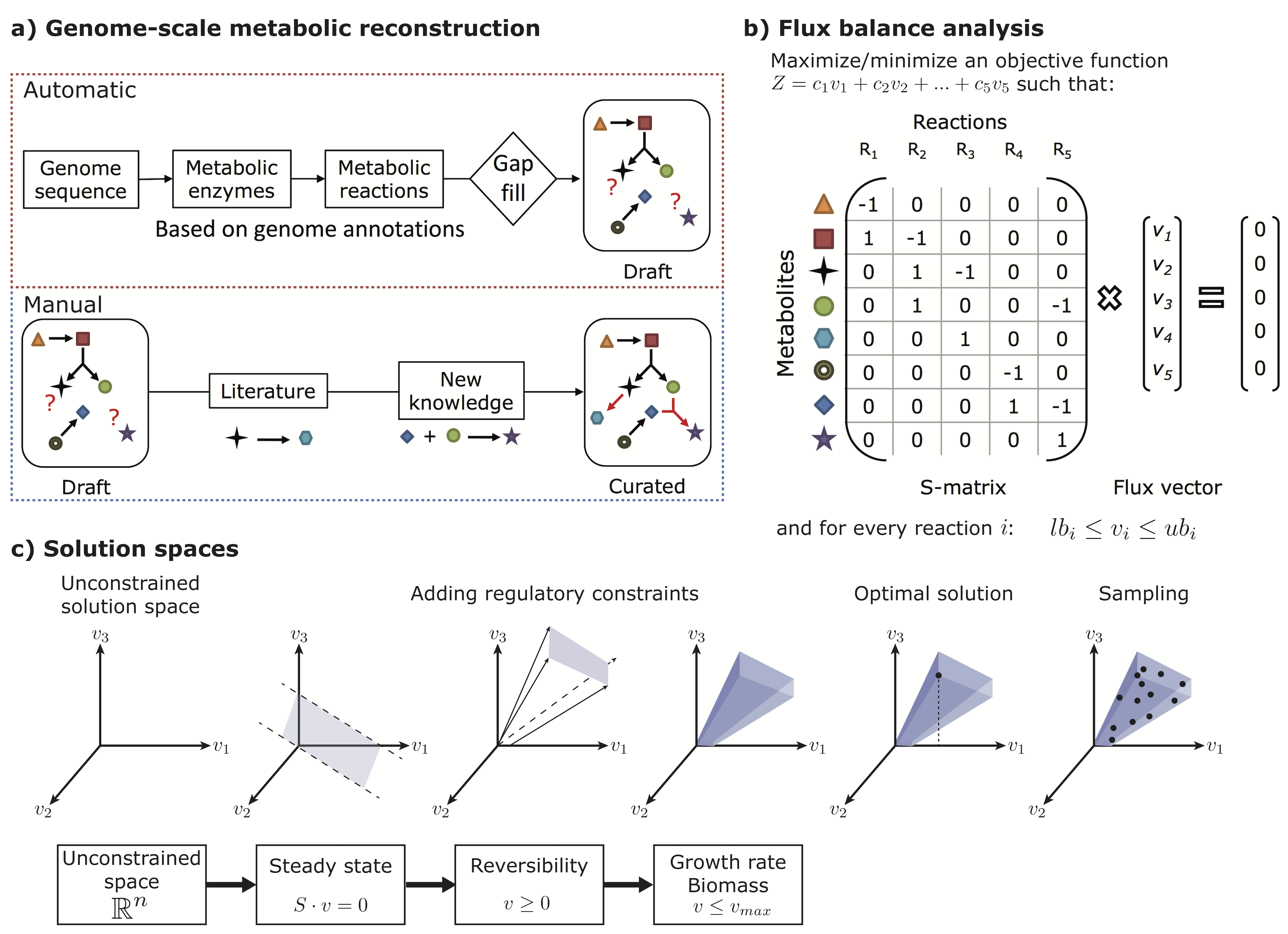
Figure 1: Illustration of genome-scale metabolic reconstruction and flux balance analysis. a. Genome-scale metabolic reconstructions are built in two steps. First, several platforms exist for the generation of a gap-filled draft metabolic reconstruction based on genome annotations. Second, the draft reconstructions need to be refined based on known experimental and biochemical data from literature[42]. Novel experiments can be performed on the organism and the reconstruction refined accordingly. b. In flux balance analysis (FBA), the metabolic reconstruction containing $n$ reactions and $m$ metabolites is converted to a stoichiometric matrix $S$. FBA solves an optimisation problem where an objective function $Z$ is maximised or minimised. $Z$ is formed by multiplying every reaction flux $v_{i}$ with a predetermined constant, $c_{i}$, and adding the resulting values. FBA solves a steady state, $Sv=0$. Every reaction $i$ is bound by two values, an upper bound ($ub_{i}$) and lower bound ($lb_{i}$). c. The solution space is defined by the mass balanced constraints imposed for the upper and lower bounds of each reaction in the metabolic reconstruction. Optimisation for a biological objective function (e.g. biomass production, ATP consumption, heme production, etc.) identifies an optimal flux within the solution space, whereas uniform sampling provides an unbiased characterisation by sampling candidate fluxes distributed in the solution space.

The present protocol is an update to the COBRA Toolbox 1.0[4] and 2.0[5] illustrating the main novel developments within version 3.0 of the COBRA Toolbox (see Table 1), especially the expansion of functionality to cover new modelling methods. In particular, this protocol includes the input and output of new standards for sharing reconstructions and models, an extended suite of supported general purpose optimisation solvers, new optimisation solvers developed especially for constraint-based modelling problems, enhanced functionality in the areas of computational efficiency and high precision computing, numerical characterisation of reconstructions, conversion of reconstructions into various forms of constraint-based models, comprehensive support for flux balance analysis and its variants, integration with omics data, uniform sampling of high dimensional models, atomic resolution of metabolic reconstructions, estimation and application of thermodynamic constraints, visualisation of metabolic networks, and genome-scale kinetic modelling.

With an increasing number of contributions from developers around the world, the code base is evolving at a fast pace. The COBRA Toolbox has evolved from monolingual MATLAB software to a multilingual software suite via integration with C, FORTRAN, Julia, Perl and Python code, as well as pre-compiled binaries, for specific purposes. For example, the integration with quadruple precision numerical optimisation solvers, implemented in FORTRAN, for robust and efficient modelling of multi-scale biochemical networks, such as those obtained with integration[7] of metabolic[8] and macromolecular synthesis[9] reconstructions, which represent a new peak in terms of biochemical comprehensiveness and predictive capacity[10]. These developments warranted an industrial approach to software development of the COBRA Toolbox. Therefore, we implemented a continuous integration approach with the aim of guaranteeing a consistent, stable, and high-quality software solution for a broad user community. All documentation and code is released as part of the openCOBRA project (https://github.com/opencobra/cobratoolbox). Where reading the extensive documentation associated with the COBRA Toolbox does not suffice, we describe the procedure for effectively engaging with the community via a dedicated online forum (https://groups.google.com/forum/#!forum/cobra-toolbox). Taken together, the COBRA Toolbox 3.0 provides an unparalleled depth of interoperable COBRA methods and a proof-of-concept that knowledge integration and collaboration by large numbers of scientists can lead to cooperative advances impossible to achieve by a single scientist or research group alone[11].

Applications of COBRA methods

Constraint-based modelling of biochemical networks is broadly applicable to a range of biological, biomedical, and biotechnological research questions[12] . Fundamentally, this broad applicability arises from the common phylogenetic tree, shared by all living organisms, that manifests in a set of shared mathematical properties that are common to biochemical networks in normal, diseased, wild-type, or mutant biochemical networks. Therefore, a COBRA method developed primarily for use in one scenario can usually be quickly adapted for use in a variety of related scenarios. Often, this adaptation retains the mathematical properties of the optimisation problem underlying the original constraint-based modelling method. By adapting the input data and interpreting the output results in a different way, the same method can be used to address a different research question.

Biotechnological applications of constraint-based modelling include the development of sustainable approaches for chemical[13] and biopharmaceutical production[14, 15]. Among these applications is the computational design of new microbial strains for production of bioenergy feedstocks from non-food plants, such as microbes capable of deconstructing biomass into their sugar subunits and synthesising biofuels, either from cellulosic biomass or through direct photosynthetic capture of carbon dioxide.

	Narrative	Novelty in the COBRA Toolbox 3.0 compared to 2.0
B	Initialise and verify the installation	Software dependency audit, e.g., solvers, binaries, git.
R	Input and output of reconstructions and models	Support for latest standards, e.g., SBML flux balance constraints[70].
R	Reconstruction: rBioNet	New software for quality controlled reconstruction[59].
R	Reconstruction: create a functional generic subnetwork	New methods for selecting different types of subnetworks.
R	Reconstruction exploration	New methods, e.g., find adjacent reactions.
R	Reconstruction refinement	Maintenance of internal model consistency, e.g., upon subnetwork generation[33].
R	Numerical reconstruction properties	Flag a reconstruction requiring a multi-scale solver[65].
R	Convert a reconstruction into a flux balance analysis model	Identification of a maximal flux and stoichiometrically consistent subset[73].
I	Atomically resolve a metabolic reconstruction	New algorithms and methods for working with molecular structures, atom mapping, identification of conserved moieties[112, 124].
I	Integration of metabolomic data	New methods for analysis of metabolomic data in a network context[71, 145].
I	Integration of transcriptomic and proteomic data	New algorithms for generation of context-specific models[91].
A	Flux balance analysis and its variants	New flux balance methods, multi-scale model rescaling and multi-scale solvers, additional solver interfaces, thermodynamically feasible methods [53, 133, 142, 129, 143, 7].
A	Variation on reaction rate bounds in flux balance analysis	Increased computational efficiency.
A	Parsimonious flux balance analysis	New method for parsimonious flux balance analysis[144].
A	Sparse flux balance analysis	New method for sparse flux balance analysis.
A	Gap filling	Increased computational efficiency[45].
A	Adding biological constraints to a flux balance model	New methods for coupling reaction rates[1, 146].
A	Testing biochemical fidelity	Human metabolic function test suite[21].
A	Testing basic properties of a metabolic model (sanity checks)	New methods to minimise occurrence of modelling artefacts[77].
A	Minimal spanning pathway vectors	New method for determining minimal spanning pathway vectors[102].
A	Elementary modes and pathway vectors	Extended functionality by integration with CellNetAnalyzer[66].
A	Minimal cut sets	Extended functionality by integration with CellNetAnalyzer[147, 148], and new algorithms for genetic MCSs [68].
A	Flux variability analysis	Increased computational efficiency[103].
A	Uniform sampling of steady-state fluxes	New algorithm, guaranteed convergence to uniform distribution[104].
A	Thermodynamically constrain reaction directionality	New algorithms and methods for estimation of thermochemical parameter estimation in multi-compartmental, genome-scale metabolic models [128, 127].
A	Variational kinetic modelling	New algorithms and methods for genome-scale kinetic modelling[72, 136, 135, 137].
D	Metabolic engineering and strain design	New methods, e.g., OptForce, interpretation of new strain designs. New modelling language interface to GAMS[149].
V	Human metabolic network visualisation: ReconMap	New method for genome-scale metabolic network visualisation[61, 62, 150].
V	Variable scope visualisation with automatic layout generation	New method for automatic visualisation of network parts[141].
	Contributing to the COBRA Toolbox with MATLAB.devTools	New software application enabling contributions by those unfamiliar with version control software.
	Engaging with the COBRA Toolbox Forum	More than 800 posted questions with supportive replies connecting problems and solutions.

Table 1: Each method available in the COBRA Toolbox 3.0 is made accessible with a narrative tutorial that illustrates how the corresponding function(s) are combined to implement each COBRA method in the respective src directories (https://github.com/opencobra/cobratoolbox/tree/master/src): analysis (A), reconstruction (R), design (D), visualisation (V), dataIntegration (I), and base (B).

Another prominent biotechnological application is the analysis of interactions between organisms that form biological communities and their surrounding environments, with a view toward utilisation of such communities for bioremediation[16] or nutritional support of non-food plants for bioenergy feedstocks. Biomedical applications of constraint-based modelling include the prediction of the phenotypic consequences of single nucleotide polymorphisms[17], drug targets[18], enzyme deficiencies [19, 20, 21, 22], as well as side and off-target effects of drugs[23, 24, 25]. COBRA has also been applied to generate and analyse normal and diseased models of human metabolism[26, 21, 27, 28, 29], including organ-specific models[30, 31, 32], multi-organ-models[33, 34], and personalised models[35, 36, 37]. Constraint-based modelling has also been applied to understanding of the biochemical pathways that interlink diet, gut microbial composition, and human health[38, 39, 40, 41, 1].

Today, genome-scale metabolic reconstructions can be automatically created using many different platforms (see the Key features and comparisons section). Automatic reconstruction tools have considerably sped up the reconstruction process, which was previously very time-consuming[42]. Various algorithms exist that facilitate gap filling of metabolic networks, e.g., SMILEY[43], GapFind[44], fastGapFill[45], SONEC[46], and EnsemblFBA[47]. Each algorithm applies a different approach and thus the gap filling solutions proposed by different algorithms may differ. However, several issues still need to be manually resolved in automatically generated and gap-filled reconstructions, e.g., ensuring stoichiometric consistency[48], thermodynamically constraining reaction directionality[49], refining gene-protein-reaction associations, and confirming experimentally determined biochemical functions of the reconstructed organism[42].

Key features and comparisons

Name	Implementation	Interface	Development	Dist.	OS
The COBRA Toolbox	MATLAB (etc)	Script/Narrative	open source⋆	git	all
RAVEN[151]	MATLAB	Script	open source⋆	git	all
CellNetAnalyzer[66]	MATLAB (etc)	Script/GUI	closed source⋆	zip	all
FBA-SimVis[152]	Java + MATLAB	GUI	closed source†	zip	Windows
OptFlux[153]	Java	Script	open source⋆	svn	all
COBRA.jl[53]	Julia	Script/Narrative	open source⋆	git	all
Sybil[64]	R package	Script	open source⋆	zip	all
COBRApy[51]	Python packages	Script/Narrative	open source⋆	git	all
CBMPy[63]	Python packages	Script	open source⋆	zip	all
Scrumpy[154]	Python packages	Script	open source⋆	tar	all
SurreyFBA[58]	C++	Script/GUI	open source⋆	zip	all
FASIMU[155]	C	Script	open source†	zip	Linux
FAME[156]	Web-based	GUI	open source†	zip	all
PathwayTools[54]	Web-based	GUI/Script	closed source⋆	N/A	all
KBase[52]	Web-based	Script/Narrative	open source⋆	git	all

Table 2: A selection of actively developed software applications with constraint-based modelling capabilities. GUI, graphical user interface. The COBRA Toolbox: https://opencobra.github.io/cobratoolbox, RAVEN: https://github.com/SysBioChalmers/RAVEN, CellNetAnalyzer: https://www2.mpi-magdeburg.mpg.de/projects/cna/cna.html, FBA-SimVis: https://immersive-analytics.infotech.monash.edu/fbasimvis, OptFlux: http://www.optflux.org, COBRA.jl: https://opencobra.github.io/COBRA.jl, Sybil: https://rdrr.io/cran/sybil, COBRApy: http://opencobra.github.io/cobrapy, CBMPy: http://cbmpy.sourceforge.net, SurreyFBA: http://sysbio.sbs.surrey.ac.uk/sfba, FASIMU: http://www.bioinformatics.org/fasimu, FAME: http://f-a-m-e.org, Pathway Tools: http://bioinformatics.ai.sri.com/ptools, KBase: https://kbase.us. The symbol ^† in the development column refers to an inactive project and the ^⋆ to an active project. The label ’all’ in the OS column means that the applications is compatible with Windows, Linux and macOS operating systems.

Besides the COBRA Toolbox, constraint-based reconstruction and analysis can be carried out with a variety of software tools. In 2012, Lakshmanan et al.[50] made a comprehensive, comparative evaluation of the usability, functionality, graphical representation and inter-operability of the tools available for flux balance analysis. Each of these evaluation criteria is still valid when comparing the current version of the COBRA Toolbox with other software with constraint-based modelling capabilities. The rapid development of novel constraint-based modelling algorithms requires continuity of software development. Short term investment in new COBRA modelling software applications has led to a plethora of COBRA modelling applications[50]. Each usually provides some unique capability initially, but many have become antiquated due to lack of maintenance, failure to upgrade, or failure to support new standards in model exchange formats (http://sbml.org/Documents/Specifications). Therefore, we also restrict our comparison to software in active development (see Table 2).

Each software tool for constraint-based modelling has varying degrees of dependency on other software. Web-based applications exist for the implementation of a limited number of standard constraint-based modelling methods. Their only local dependency is on a web browser. The COBRA Toolbox depends on MATLAB (Mathworks Inc.), a commercially distributed, general-purpose computational tool. MATLAB is a multi-paradigm programming language and numerical computing environment that allows matrix manipulations, plotting of functions and data, implementation of algorithms, creation of user interfaces, and interfacing with programs written in other languages, including C, C++, C#, Java, Fortran, and Python. All software tools for constraint-based modelling also depend on at least one numerical optimisation solver. The most robust and efficient numerical optimisation solvers for standard problems are distributed commercially, but often with free licences available for academic use, e.g., Gurobi Optimizer (http://www.gurobi.com). Stand-alone constraint-based modelling software tools also exist and their dependency on a numerical optimisation solver is typically satisfied by GLPK (https://gnu.org/software/glpk), an open-source linear optimisation solver.

It is sometimes perceived that there is a commercial advantage to depending only on open-source software. However, there are also commercial costs associated with dependency on open-source software. That is, in the form of increased computation times as well as increased time required to install, maintain and upgrade open-source software dependencies. This is an important consideration for any research group whose primary focus is on biological, biomedical, or biotechnological applications, rather than on software development. The COBRA Toolbox 3.0 strikes a balance by depending on closed-source, general purpose, commercial computational tools, yet all COBRA code is distributed and developed in an open-source environment (https://github.com/opencobra/cobratoolbox).

The availability of comprehensive documentation is an important feature in the usability of any modelling software. Therefore, a dedicated effort has been made to ensure that all functions in the COBRA Toolbox 3.0 are comprehensively and consistently documented. Moreover, we also provide a new suite of more than 35 tutorials (https://opencobra.github.io/cobratoolbox/latest/tutorials) to enable beginners, as well as intermediate and advanced users to practise a wide variety of COBRA methods. Each tutorial is presented in a variety of formats, including as a MATLAB live script, which is an interactive document, or narrative, (https://mathworks.com/help/matlab/matlab_prog/what-is-a-live-script.html) that combines MATLAB code with embedded output, formatted text, equations, and images in a single environment viewable with the MATLAB Live Editor (version R2016a or later). MATLAB live scripts are similar in functionality to Mathematica Notebooks (Wolfram Inc.) and Jupyter Notebooks (https://jupyter.org). The latter support interactive data science and scientific computing for more than 40 programming languages. To date, only the COBRA Toolbox 3.0, COBRApy[51], KBase[52], and COBRA.jl[53] offer access to constraint-based modelling algorithms via narratives.

KBase is a collaborative, open environment for systems biology of plants, microbes and their communities[52]. It also has a suite of analysis tools and data that support the reconstruction, prediction, and design of metabolic models in microbes and plants. These tools are tailored toward the optimisation of microbial biofuel production, the identification of minimal media conditions under which that fuel is generated, and predict soil amendments that improve the productivity of plant bioenergy feedstocks. In our view, KBase is currently the tool of choice for the automatic generation of draft microbial metabolic networks, which can then be imported into the COBRA Toolbox for further semi-automated refinement, which has recently successfully been completed for a suite of gut microbial organisms[1]. However, KBase[52] currently offers a modest depth of constraint-based modelling algorithms.

MetaFlux[54] is a web-based tool for the generation of network reconstructions directly from pathway and genome databases, proposing network refinements to generate functional flux balance models from reconstructions, predict steady-state reaction rates with flux balance analysis and interpret predictions in a graphical network visualisation. MetaFlux is tightly integrated within the PathwayTools[55] environment, which provides a broad selection of genome, metabolic and regulatory informatics tools. As such, PathwayTools provides breadth in bioinformatics and computational biology, while the COBRA Toolbox 3.0 provides depth in constraint-based modelling, without providing, for example, any genome informatics tools. Although an expert can locally install a PathwayTools environment, the functionality is closed source and only accessible via an application programming interface. This approach does not permit the level of repurposing possible with open-source software. As recognised in the computational biology community [56], open-source development and distribution is scientifically important for tractable reproducibility of results as well as reuse and repurposing of code [57].

Lakshmanan et al.[50] consider the availability of a graphical user interface to be an important feature in the usability of modelling software. For example, SurreyFBA[58] provides a command line tool and graphical user interface for constraint-based modelling of genome-scale metabolic reaction networks. The time lag between the development of a new modelling method and its availability via a graphical user interface necessarily means that graphically driven COBRA tools permit a limited depth of novel constraint-based modelling methods. While MATLAB provides a generic graphical user interface, the COBRA Toolbox is controlled either by scripts or narratives, rather than graphically. Exceptions include the input of manually-curated data during network reconstruction[59], the assimilation of genome-scale metabolic reconstructions[60], and the visualisation of simulation results in biochemical network maps[61] via specialised network visualisation software[62].

Due to the relative simplicity of the MATLAB programming language, new COBRA Toolbox users, including those without software development experience, can rapidly become familiar with the basics of constraint-based modelling. This initial learning effort is worth it for the flexibility it opens up, especially considering the broad array of constraint-based modelling methods now available within the COBRA Toolbox 3.0. Although it should be technically possible to generate a computational specification of the point-and-click analysis steps that are required to generate results using a graphical user interface, to our knowledge, none of the graphically-driven modelling tools in Table 2 offers this facility. Such a specification would be required for another scientist to reproduce the same results using the same tool. This weakness limits the ability to reproduce analytical results, as verbal specification is not sufficient for reproducibility[57].

Each language-specific COBRA implementation has its benefits and drawbacks, which are mainly associated with the programming language itself. PySCeS-CBM[63] and COBRApy[51] both provide support for a set of COBRA methods implemented in the Python programming language. Python is a multi-paradigm, interpreted programming language for general-purpose programming. It has a broad development community and a wide range of open-source libraries, especially in bioinformatics. As such, it is well suited for the amalgamation and management of heterogeneous experimental data. At present, the COBRA software tools in Python provide access to standard COBRA methods. In COBRApy[51], this functionality can be extended by using Python to invoke MATLAB and use the COBRA Toolbox. Achieving such interoperability between COBRA software implemented in different programming languages and developed together by a united open source community is the primary objective of the openCOBRA project (https://opencobra.github.io).

Sybil[64] is an open-source, object-oriented software library that implements a limited set of standard constraint-based modelling algorithms in the programming language R, which is a free, platform independent environment for statistical computing and graphics. Sybil is available for download from the comprehensive R archive network (CRAN), but does not follow an open-source development model. The COBRA Toolbox is primarily implemented in MATLAB, a proprietary, multi-paradigm, programming language which is interpreted for execution rather than compiled prior to execution. As such, MATLAB code typically runs slower than compiled code, but the main advantage is the ability to rapidly and flexibly implement sophisticated numerical computations by leveraging the extensive libraries for general-purpose numerical computing, supplied commercially within MATLAB (Mathworks Inc.), and distributed freely by the community (https://mathworks.com/matlabcentral).

For the application of computationally-demanding constraint-based modelling methods to high-dimensional or high-precision constraint-based models, the COBRA Toolbox 3.0 comes with an array of integrated, pre-compiled extensions and interfaces that employ complementary programming languages and tools. These include a quadruple precision Fortran 77 optimisation solver implementation for constraint-based modelling of multi-scale biochemical networks[65], and a high-level, high-performance, open-source implementation of flux balance analysis in Julia [53]. The latter is tailored to solve multiple flux balance analyses on a subset or all the reactions of large- and huge-scale networks, on any number of threads or nodes. To enumerate elementary modes or minimal cut-sets, we provide an interface to CellNetAnalyzer[66, 67] (https://www2.mpi-magdeburg.mpg.de/projects/cna/cna.html), which excels at computationally-demanding, enumerative, discrete geometry calculations of relevance to biochemical networks. In addition, we included an updated implementation of the genetic minimal cut-sets approach [68], which extends the concept of minimal cut-sets to gene knockout interventions.

In summary, the COBRA Toolbox 3.0 provides an unparalleled depth of constraint-based reconstruction and analysis methods, has a highly active and supportive open-source development community, is accompanied by extensive documentation and narrative tutorials, it leverages the most comprehensive library for numerical computing, and it is distributed with extensive interoperability with a range of complementary programming languages that exploit their particular strengths to realise specialised constraint-based modelling methods. A list of the main COBRA methods now available in the COBRA Toolbox is given in Table 1. Moreover, all of this functionality is provided within one accessible software environment.

Experimental Design

The COBRA Toolbox 3.0 is designed for flexible adaptation into customised pipelines for constraint-based reconstruction and analysis in a wide range of biological, biochemical, or biotechnological scenarios, from single organisms to communities of organisms. To become proficient in adapting the COBRA Toolbox to generate a protocol specific to one’s situation, it is wise to first familiarise oneself with the principles of constraint-based modelling. This can best be achieved by studying the educational material already available. The textbook Systems Biology: Constraint-based Reconstruction and Analysis[2] is an ideal place to start. It is accompanied by a set of lecture videos that accompany each chapter http://systemsbiology.ucsd.edu/Publications/Books/SB1-2LectureSlides. The textbook Optimization Methods in Metabolic Networks[69] provides the fundamentals of mathematical optimisation and its application in the context of metabolic network analysis. A study of this educational material will accelerate one’s ability to utilise any software application dedicated to COBRA.

Once one is cognisant of the conceptual basis of COBRA, one can then proceed with this protocol, which summarises a subset of the key methods that are available within the COBRA Toolbox. To adapt this protocol to one’s situation, users can combine the COBRA methods implemented within the COBRA Toolbox in numerous ways. The adaption of this protocol to one’s situation may require the development of new customised MATLAB scripts that combine existing methods in a new way. Due to the aforementioned benefits of narratives, the first choice should be to implement these customised scripts in the form of MATLAB live scripts. To get started, the existing tutorial narratives, described in Table 1, can be repurposed as templates for new analysis pipelines. Narrative figures and tables can then be used within the main text of scientific articles and converted into supplementary material to enable full reproducibility of computational results. The narratives specific to individual scientific articles can also be shared with peers within https://github.com/opencobra/cobratoolbox/tree/master/papers. New tutorials can be shared with the COBRA community by contributing to the future development of the COBRA Toolbox (cf. the Software architecture section). Depending on one’s level of experience, or the novelty of an analysis, the adaptation of this protocol to a particular situation may require the adaption of existing COBRA methods, or development of new COBRA methods, or both.

Field name	Size	Data Type	Field description
.b	$m\times 1$	double	The coefficients of the constraints of the metabolites ($Sv=b$).
ense	$m\times 1$	char	The sense of the constraints represented by $b$, each row is either 'E' (equality), 'L' (less than) or 'G' (greater than).
tCharges	$m\times 1$	numeric	The charge of the respective metabolite ( if unknown).
tFormulas	$m\times 1$	cell of char	Elemental formula for each metabolite.
tInChIString	$m\times 1$	cell of char	Formula for each metabolite in the InCHI strings format.
tNames	$m\times 1$	cell of char	Full name of each corresponding metabolite.
ts	$m\times 1$	cell of char	Identifiers of the metabolites.
tSmiles	$m\times 1$	cell of char	Formula for each metabolite in SMILES Format.
.c	$n\times 1$	double	The objective coefficient of the reactions.
Rules	$n\times 1$	cell of char	A string representation of the GPR rules defined in a readable format.
	$n\times 1$	double	Lower bounds for fluxes through the reactions.
nConfidenceScores	$n\times 1$	numeric	Confidence scores for reaction presence (0-5, with 5 being the highest confidence).
nECNumbers	$n\times 1$	cell of char	E.C. number for each reaction.
nNames	$n\times 1$	cell of char	Full name of each corresponding reaction.
nNotes	$n\times 1$	cell of char	Description of each corresponding reaction.
nReferences	$n\times 1$	cell of char	Description of references for each corresponding reaction.
ns	$n\times 1$	cell	Identifiers of the reactions.
bSystems	$n\times 1$	cell of cell of char	subSystem assignments for each reaction.
	$n\times 1$	double	Upper bounds for fluxes through the reactions.
.S	$m\times n$	numeric	The stoichiometric matrix containing the model structure (for large models a sparse format is suggested).
neNames	$g\times 1$	cell of char	Full name of each corresponding gene.
nes	$g\times 1$	cell of char	Identifiers of the genes in the model.
oteinNames	$g\times 1$	cell of char	Full name for each protein.
oteins	$g\times 1$	cell of char	Proteins associated with each gene (one protein per gene).
nGeneMat	$n\times g$	numeric or logical	Matrix with rows corresponding to reactions and columns corresponding to genes.
mpNames	$c\times 1$	cell of char	Descriptions of the Compartments (pNames(m) is associated with ps(m)).
mps	$c\times 1$	cell of char	Symbols for compartments.
enseStr	$1\times 3$	char	The objective sense: either 'max' (maximisation) or 'min' (minimisation).

Table 3: A description of the main fields of a standard model structure.

Software architecture of the COBRA Toolbox 3.0

The source code of the COBRA Toolbox (https://github.com/opencobra/cobratoolbox/tree/master/src) is divided into several top-level folders, which either mimic the main classes of COBRA methods (reconstruction, dataIntegration, analysis, visualisation, design) or contain the basic functions (base) available for use within many COBRA methods. For example, the input or output of reconstructions and models in various formats as well as all the interfaces to optimisation solvers is contained within the base folder. The reconstruction folder contains all of the methods associated with the reconstruction and refinement of a biochemical network to match experimental data, as well as the conversion of a reconstruction into various forms of constraint-based models (see Table 3 for a description of the main fields of a COBRA model). The dataIntegration folder contains the methods for integration of metabolomic, transcriptomic, proteomic, and thermodynamic data with a reconstruction or model. The analysis folder contains all of the methods for interrogation of the properties of a reconstruction or model, and combinations thereof, as well as the prediction of biochemical network states using constraint-based models. The visualisation folder contains all of the methods for the visualisation of predictions within a biochemical network context, using various biochemical cartography tools that interoperate with the COBRA Toolbox. The design folder contains new strain design methods and a new modelling language interface to GAMS.

Open-source software development with the COBRA Toolbox

Understanding how the COBRA Toolbox is developed is most important for developers, so beginners may skip this section at first. The COBRA Toolbox is version controlled using Git (https://git-scm.com), a free and open-source distributed, version control system, which tracks changes in computer files and is used for coordinating work on those files by multiple people. The continuous integration environment facilitates contributions from the fork of COBRA developers to a development branch, whilst ensuring that robust, high-quality, well-tested code is released to end users on the master branch. To lower the technological barrier to the use of the aforementioned software development tools, we have developed MATLAB.devTools (https://github.com/opencobra/MATLAB.devTools), a new user-friendly software extension that enables submission of new COBRA software and tutorials. A server-side, semi-automated continuous integration environment ensures that the code in each new submission is first verified automatically, via a comprehensive test suite that detects bugs and integration errors, and second, is reviewed manually by at least one domain expert, before integration with the development branch. Thirdly, each new contribution to the development branch is evaluated in practice by active COBRA researchers, before it becomes part of the master branch.

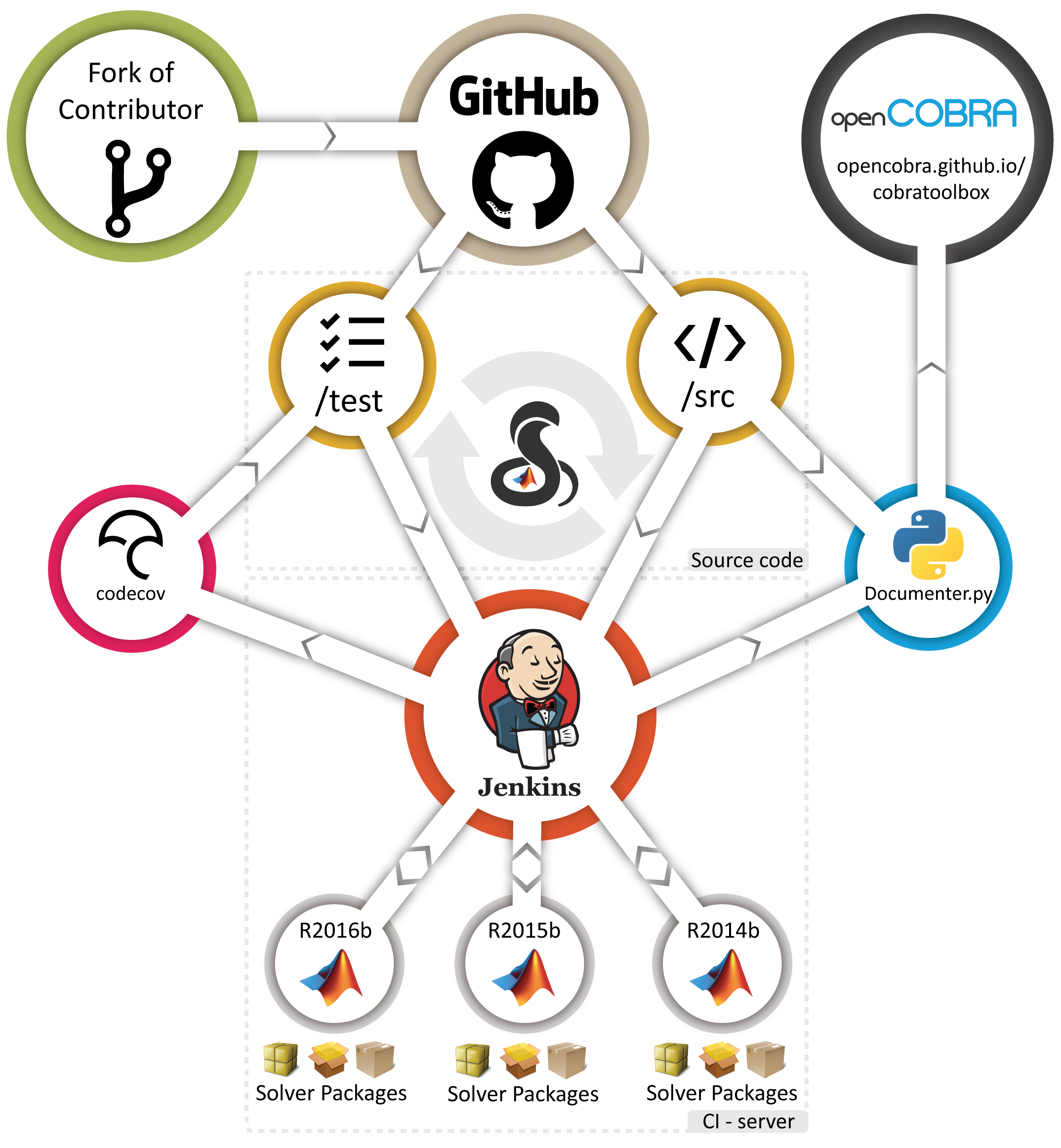
Figure 2: Continuous integration is performed on a dedicated server running Jenkins (https://jenkins.io). The main code is located in the src folder and tests functions in the test folder. A test not only runs a function (first degree testing), but tests the output of that function (second degree testing). The continuous integration setup relies on end-of-year releases of MATLAB only. Soon after the latest stable version of MATLAB is released, full support will be provided for the COBRA Toolbox. After a successful run of tests on the three latest end-of-year releases of MATLAB using various solver packages, the documentation based on the headers of the functions (docstrings) is extracted, generated, and automatically deployed. Immediate feedback through code coverage reports (%****␣intro.tex␣Line␣650␣****https://codecov.io/gh/opencobra/cobratoolbox) and build statuses are reported on GitHub. With this setup, the impact of local changes in the code base is promptly revealed.

Until recently, the code quality checks of the COBRA Toolbox have been primarily static: the code has been reviewed by experienced users and developers while occasional code inspections led to discoveries of bugs. The continuous integration setup defined in Figure 2 aims at dynamic testing with automated builds, code evaluation, and documentation deployment. Often, a function runs properly independently and yields the desired output(s), but when called within a different part of the code, logical errors are thrown. The unique advantage of continuous integration is that logical errors are mostly avoided.

Besides automatic testing, manual usability testing is performed regularly by users and is key to provide a tested and usable code base to the end user. These users provide feedback on the usability of the code base, as well as the documentation, and report eventual issues online (https://github.com/opencobra/cobratoolbox/issues). The documentation is automatically deployed to https://opencobra.github.io/cobratoolbox based on function headers. Moreover, each of the narrative tutorials is presented in a format suitable for web browsers (https://opencobra.github.io/cobratoolbox/latest/tutorials).

Controls

COBRA is part of an iterative systems biology cycle[2]. As such, it can be used as a framework for integrative analysis of experimental data in the context of prior information on the biochemical network underlying one or many complementary experimental datasets. Moreover, it can be used to predict the outcome of new experiments, or it can be used in both of these scenarios at once. Assuming all of the computational steps are errorless, the appropriate control for any prediction derived from a computational model is the comparison with independent experimental data, that is, experimental data that was not used for the model-generated predictions. It is also important to introduce quality controls to check that the computational steps are free from certain errors that may arise during adaptation of existing COBRA protocols or development of new ones.

There are various strategies for the implementation of computational quality controls. Within the COBRA Toolbox 3.0, significant effort has been devoted to automatically test the functionality of existing COBRA methods. We have also embedded a large number of sanity checks, which evaluate whether the input data could possibly be appropriate for use with a function. These sanity checks have been accumulated over more than a decade of continuous development of the COBRA Toolbox. Their objective is to rule out certain known classes of obviously false predictions that might result from an inappropriate use of a COBRA method, but they do not (and are not intended) to catch every such error, as it is impossible to imagine all of the eventual erroneous inputs that may be presented to a COBRA Toolbox function. It is advisable to add own narratives with additional sanity checks, which will depend heavily on the modelling scenario.

Required expertise

Most of this protocol can be implemented by anyone with a basic familiarity with the principles of constraint-based modelling. Some methods are only for advanced users. If one is a beginner with respect to MATLAB, Supplementary Manual 1 provides pointers to get started. MATLAB is a relatively simple programming language to learn, but it is also a powerful language for an expert due to the large number of software libraries for numerical and symbolic computing that it provides access to. Certain specialised methods within this protocol, such as thermodynamically constraining reaction directionality, depend on the installation of other programming languages and software, which may be too challenging for a beginner with a non-standard operating system.

If the documentation and tutorials provided within the COBRA Toolbox are not sufficient, then Steps Engaging with the COBRA Toolbox forum  TIMING $1-10^{2}$ s and Engaging with the COBRA Toolbox forum  TIMING $1-10^{2}$ s guide the user toward sources of COBRA community support. The computational demands associated with the implementation of this protocol for one’s reconstruction or model of choice is dependent on the size of the network concerned. For a genome-scale model of metabolism, usually a desktop computer is sufficient. However, for certain models, such as a community of genome-scale metabolic models, a multi-scale model of metabolism and macromolecular synthesis, or a multi-tissue model, more powerful processing and extensive memory capacity is required, ranging from a workstation to a dedicated computational cluster. Embarrassingly parallel, high-performance computing is feasible for most model analysis methods implemented in the COBRA Toolbox, which will run in isolation with invocation from a distributed computing engine. It is currently an ongoing topic of research, beyond the scope of this protocol, to fully exploit high-performance computing environments with software developed within the wider openCOBRA environment, though some examples[53] are already available for interested researchers to consult.

Limitations

A protocol for the generation of a high-quality, genome-scale reconstruction, using various software applications, including the COBRA Toolbox, has previously been disseminated[42]; therefore, this protocol focuses more on modelling than reconstruction. The COBRA Toolbox is not meant to be a general-purpose computational biology tool as it is focussed on constraint-based reconstruction and analysis. For example, although various forms of generic data analysis methods are available within MATLAB, the input data for integration with reconstructions and models within the COBRA Toolbox is envisaged to have already been preprocessed by other tools. Within its scope, the COBRA Toolbox aims for complete coverage of COBRA methods. The first comprehensive overview of the COBRA methods available for microbial metabolic networks[6] requires an update to encompass many additional methods that have been reported to date, in addition to the COBRA methods targeted toward other biochemical networks. The COBRA Toolbox 3.0 provides the most extensive coverage of published COBRA methods. However, there are certainly some methods that have yet to be incorporated directly as MATLAB implementations, or indirectly via a MATLAB interface to a software dependency. Although in principle any COBRA method could be implemented entirely within MATLAB, it may be more efficient to leverage the core strength of another programming language that could provide intermediate results that can be incorporated into the COBRA Toolbox via various forms of MATLAB interfaces. Such a setup would enable one to overcome any current limitation in coverage of existing methods.

Overview

This protocol consists of a set of methods that are introduced in sequence but can be combined in a multitude of ways. The overall purpose is to enable the user to generate a biologically relevant, high-quality model that enables novel predictions and hypotheses generation. Therefore, we implement and enforce standards in reconstruction and simulation that have been developed by the COBRA community over the past two decades. All explanations of a method are also accompanied by explicit computational commands.

First, we explain how to initialise and verify the installation of the COBRA Toolbox in MATLAB (Mathworks, Inc.). The main options to import and explore the content of a biochemical network reconstruction are introduced. For completeness, a brief summary of methods for manual and algorithmic reconstruction refinement are provided, with reference to the established reconstruction protocol [42]. We also explain how to characterise the numerical properties of a reconstruction, especially with respect to detection of a reconstruction requiring a multi-scale numerical optimisation solver. We explain how to semi-automatically convert a reconstruction into a constraint-based model suitable for flux balance analysis. This is followed by an extensive explanation of how to carry out flux balance analysis and its variants. The procedure to fill gaps in a reconstruction, due to missing reactions, is also explained.

We provide an overview of the main methods to integrate metabolomic, transcriptomic, proteomic, and thermochemical data to generate context-specific, constraint-based models. Various methods are explained for the addition of biological constraints to a constraint-based model. We then explain how to test the chemical and biochemical fidelity of the model. Now that a high-quality model is generated, we explain how to interrogate the discrete geometry of its stoichiometric subspaces, how to efficiently measure the variability associated with the prediction of steady state reaction rate using flux variability analysis, and how to uniformly sample steady-state fluxes. We introduce various approaches for prospective uses of a constraint-based model, such as strain and experimental design.

We explain how to atomically resolve a metabolic reconstruction by connecting it with molecular species structures and how to use cheminformatic algorithms for atom mapping and identification of conserved moieties. Using molecular structures for each metabolite, and established thermochemical data, we estimate the transformed Gibbs energy of each subcellular compartment specific reaction in a model of human metabolism in order to thermodynamically constrain reaction directionality and constrain the set of feasible kinetic parameters. Sampled kinetic parameters are then used for variational kinetic modelling, in an illustration of the utility of recently published algorithms for genome-scale kinetic modelling. We also explain how to visualise predicted phenotypic states using a recently developed approach for metabolic network visualisation. We conclude with an explanation of how to engage with the community of COBRA developers, as well as contribute code to the COBRA Toolbox with MATLAB.devTools, a newly developed piece of software for community contribution of COBRA methods to the COBRA Toolbox.

MATERIALS

Equipment

Required hardware

• A computer with any 64-bit Intel or AMD processor and at least 8 GB of RAM. ! CAUTION

  Depending on the size of the reconstruction or model, more processing power and more memory may be needed, especially if it is also desired to store the results of analysis procedures within the MATLAB workspace.

• A hard drive with free storage of at least 10 GB.

• ! CAUTION A working and stable internet connection is required during installation and while contributing to the COBRA Toolbox.

Required software

• A Linux, macOS or Windows operating system that is MATLAB qualified (https://mathworks.com/support/sysreq.html).

• MATLAB (MathWorks Inc. - https://mathworks.com/products/matlab.html), version R2014b or above is required. Version R2016a or above is required for running MATLAB live scripts (tutorials .mlx files). Note that the tutorials can be run on R2014b using the provided .m files. ! CAUTION No support is provided for versions older than R2014b. MATLAB is released on a twice-yearly schedule. After the latest release (version b), it may be a couple of months before certain methods with dependencies on other software become compatible. For example, the latest releases of MATLAB may not be compatible with the existing solver interfaces, necessitating an update of the MATLAB interface provided by the solver developers, or an update of the COBRA Toolbox, or both.

• The COBRA Toolbox (https://github.com/opencobra/cobratoolbox) version 3.0 or above.

• A working bash terminal (or shell) with UNIX tools. curl version 7.0 or above must be installed to ensure connectivity between the COBRA Toolbox and the remote Github server. The version control software git 1.8 or above is required to be installed and accessible through system commands. ! CAUTION On Windows, the shell integration included with git Bash (https://git-for-windows.github.io) utilities must be installed. On macOS, a working installation of Xcode (https://developer.apple.com/xcode) version 8.0 or above and command line tools is mandatory.

Optional software

The following third-party software and MATLAB toolboxes are only required for one or more optional steps of the procedure.

• Reading and writing models in SBML (Systems Biology Markup Language) format requires the MATLAB interface from the libSBML application programming interface, version 5.15.0 or above. The COBRA Toolbox 3.0 supports the latest SBML Level 3 Flux Balance Constraints Version 2 package (http://sbml.org/Documents/Specifications/SBML_Level_3/Packages/fbc). The COBRA Toolbox developers work closely with the SBML Team to ensure that the COBRA Toolbox supports the latest standards, and moreover that standard development is also focused on meeting the evolving requirements of the constraint-based modelling community. ! CAUTION After the latest release of MATLAB, there may be a short time lag before input and output become fully compatible. For example, the input and output of .xml files in the SBML standard formats relies on platform dependent binaries that we maintain (https://github.com/opencobra/COBRA.binary) for each major platform, but the responsibility for maintenance of the source code [70] lies with the SBML team (http://sbml.org), who have a specific forum for raising interoperability issues (https://groups.google.com/forum/#!forum/sbml-interoperability).

• The MATLAB Image Processing Toolbox, the Parallel Computing Toolbox, the Statistics and Machine Learning Toolbox, and the Optimization Toolbox and Bioinformatics Toolbox (https://mathworks.com/products) must be licensed and installed to ensure certain model analysis functionality, such as topology based algorithms, flux variability analysis, or sampling algorithms.

• The Chemaxon Calculator Plugins (https://chemaxon.com/products/calculator-plugins - ChemAxon Ltd), version 16.9.5.0 or above, is a suite offering a range of cheminformatics tools. Standardizer is ChemAxon’s solution to transform chemical structures into customised, canonical representations to achieve best reliability with chemical databases. A licence is freely available for academics.

• Java (https://java.com/en/download/help/download_options.xml), version 8 or above, is a programming language which enables platform independent applications.

• Python (https://python.org/downloads), version 2.7, is a high-level programming language for general-purpose programming and is required to run NumPy or generate the documentation locally (relevant when contributing).

• NumPy (https://scipy.org/install.html), version 1.11.1 or above, is the fundamental package for scientific computing with Python.

• OpenBabel (https://openbabel.org), version 2.3 or above, is a chemical toolbox designed to speak the many languages of chemical data.

• Reaction Decoder Tool (RDT - https://github.com/asad/ReactionDecoder/releases), version 1.5.0 or above, is a Java-based, open-source atom mapping software tool.

Solvers

Table 4 provides an overview of supported optimisation solvers. For optimal performance, we recommend to install an industrial-strength numerical optimisation solver. At least one linear programming (LP) solver is required for basic constraint-based modelling methods. By default, the COBRA Toolbox installs the free LP and MILP solver GLPK (https://gnu.org/software/glpk) as well as DQQ, MINOS, PDCO, and QPNG. On Windows, the OPTI solver suite (https://inverseproblem.co.nz/OPTI) must be installed separately in order to use the OPTI interface. ! CAUTION Depending on the type of optimisation problem underlying a COBRA method, an additional numerical optimisation solver may be required.

	Name	Version	Interface	LP	MILP	QP	MIQP	NLP
Active Support	DQQ	-	dqqMinos	$\star$
	GLPK	2.7+	glpk	$\star$	$\star$
	GUROBI	7.0+	gurobi	$\star$	$\star$	$\star$	$\star$
	ILOG CPLEX	12.7.1+	ibm_cplex	$\star$	$\star$	$\star$
	MATLAB	R2014b+	matlab	$\star$				$\star$
	MINOS	-	quadMinos	$\star$				$\star$
	MOSEK	8.0+	mosek	$\star$	$\star$	$\star$
	PDCO	-	pdco	$\star$		$\star$		$\star$
	Tomlab CPLEX	8.0+	cplex_direct	$\star$	$\star$	$\star$	$\star$
			tomlab_cplex	$\star$	$\star$	$\star$	$\star$
Passive	OPTI	2.27+	opti	$\star$	$\star$	$\star$	$\star$	$\star$
	QPNG	-	qpng			$\star$
	Tomlab SNOPT	8.0+	tomlab_snopt					$\star$
Legacy	GUROBI	7.0+	gurobi_mex	$\star$	$\star$	$\star$	$\star$
	LINDO	2.0+	lindo_old	$\star$
			lindo_legacy	$\star$
	MATLAB	R2014b+	lp_solve	$\star$

Table 4: An overview of the types of optimisation problems solved by each optimisation solver. The interface to certain standard optimisation solvers is actively supported, whereas the interface to other non-standard solvers requires testing by the end user to ensure compatibility, while a legacy solver interface might require refinement before it becomes compatible with newer solver or MATLAB releases.

Application specific software

Certain solvers have additional software requirements, and some binaries provided in the COBRA.binary (https://github.com/opencobra/COBRA.binary) repository might not be compatible with your system.

• The dqqMinos and Minos solvers may only be used on Unix. The C-shell csh (http://bxr.su/NetBSD/bin/csh) is required.

• The GNU C-compiler gcc 7.0 or above (https://gcc.gnu.org). The library of the gcc compiler is required for generating new binaries of fastFVA with a different version of the CPLEX solver than officially supplied. The GNU Fortran compiler gfortran 4.1 or above (https://gcc.gnu.org/fortran). The library of the gfortran compiler is required for running dqqMinos.

Contributing software

• MATLAB.devTools (https://github.com/opencobra/MATLAB.devTools) is highly recommended for contributing code to the COBRA Toolbox in a user-friendly and convenient way, even for those without basic knowledge of git.

Equipment setup

Required software

Here we describe specific installation instructions for software described in previous sections.

• ! CAUTION Make sure that the operating system is compatible with the MATLAB version by checking the requirements on https://mathworks.com/support/sysreq/previous_releases.html. Follow the upgrade and installation procedures on the supplier’s website or ask your system administrator for help if required.

• Install MATLAB and its licence by following the official installation instructions (https://mathworks.com/help/install/ug/install-mathworks-software.html) or ask your system administrator.

• Install the COBRA Toolbox by following the procedures given on https://github.com/opencobra/cobratoolbox. ! CAUTION Make sure that all system requirements outlined under https://opencobra.github.io/cobratoolbox/docs/requirements.html are met. If an installation of the COBRA Toolbox is already present, there is no need to re-clone the full repository. Instead, you can update the repository from MATLAB or from the terminal.

  1. Update from within MATLAB by running:

     ⬇

     updateCobraToolbox

  2. Update from the terminal (or shell) by running from within the cobratoolbox directory

     ⬇

     d cobratoolbox # change to the cobratoolbox directory

     $ git checkout master # switch to the master branch

     $ git pull origin master # retrieve changes

  CRITICAL STEP

  The official repository must be cloned as explained in the installation instructions in Steps Contributing to the COBRA Toolbox with MATLAB.devTools   TIMING $1-30$ s-7. The COBRA Toolbox can only be updated if no changes have been made locally in the cloned repository. Steps Contributing to the COBRA Toolbox with MATLAB.devTools   TIMING $1-30$ s-7 provide explanations on how to contribute.

  In case the update of the COBRA Toolbox fails or cannot be completed, clone the repository again.

• On Linux and macOS, a bash terminal with git and curl is readily available. Supplementary Manual 2 provides a brief guide to the basics of using a terminal. ! CAUTION On Windows, the command line tools such as git or curl will be be installed together with git Bash. Make sure that you select <Use git Bash and optional Unix tools from the Windows Command prompt during the installation process> of git Bash. After installing git Bash, restart MATLAB. On macOS, install the Xcode command line tools by following the instructions on https://railsapps.github.io/xcode-command-line-tools.html.

Optional software

Some software is only required for one or more optional steps of the procedure.

• The libSBML package, version 5.15.0 or above is already packaged with the COBRA Toolbox via the COBRA.binary submodule for all common operating systems. Alternatively, binaries can be downloaded separately and installed by following the procedure on http://sbml.org/Software/libSBML.

• The individual MATLAB toolboxes can be installed during the MATLAB installation process. If MATLAB is already installed, the toolboxes can be managed using the built-in MATLAB add-on manager as described on https://mathworks.com/help/matlab/matlab_env/manage-your-add-ons.html.

• The Chemaxon Calculator Plugins, version 16.9.5.0 or above can be installed by following the installation procedures outlined in the user guide on https://chemaxon.com/products/calculator-plugins.

• Install Java, version 8 or above, by following the procedures given on https://java.com/en/download/help/index_installing.xml.

• Python, version 2.7 is already installed on Linux and macOS. On Windows, follow the instructions on https://wiki.python.org/moin/BeginnersGuide/Download.

• NumPy may be installed by following the procedures on https://docs.scipy.org/doc/numpy-1.10.1/user/install.html.

• OpenBabel, version 2.3 or above, may be installed by following the installation instructions on http://openbabel.org/wiki/Category:Installation.

• Latest version of the Reaction Decoder Tool (RDT) can be installed by following the procedures on https://github.com/asad/ReactionDecoder#installation.

Most steps of the solver installation require superuser or administrator rights (
o) and eventually setting environment variables. Detailed instructions and links to the official installation guidelines for installing Gurobi, Mosek, Tomlab and IBM Cplex can be found on https://opencobra.github.io/cobratoolbox/docs/solvers.html. ! CAUTION Make sure that environment variables are properly set in order for the solvers to be properly recognised by the COBRA Toolbox.

Application specific software

• On Linux or macOS, the C-shell csh can be installed by following the instructions on https://en.wikibooks.org/wiki/C_Shell_Scripting/Setup.

• The gcc and gfortran compilers can be installed by following the links given on https://opencobra.github.io/cobratoolbox/docs/compilers.html.

Contributing software

• The MATLAB.devTools can be installed by following the instructions given on https://github.com/opencobra/MATLAB.devTools#installation. Alternatively, if the COBRA Toolbox is already installed, then the MATLAB.devTools can be installed directly from within MATLAB by typing:

  ⬇

  installDevTools()

PROCEDURE

Initialisation of the COBRA Toolbox   TIMING $5-30$ s

1$\leavevmode\nobreak\ |$  At the start of each MATLAB session, the COBRA Toolbox must be initialised. The initialisation can be done either manually (option A) or automatically (option B).

1. Automatically initialising the COBRA Toolbox

   For a regular user who primarily uses the official openCOBRA repository, automatic initialisation of the COBRA Toolbox is recommended.

   1. Edit the MATLAB startup.m file and add a line with
      tCobraToolbox so that the COBRA Toolbox is initialised each time that MATLAB is started.

      ⬇

      edit startup.m

1. Manually initialising the COBRA Toolbox

   It is highly recommended to manually initialise when contributing (see Steps Contributing to the COBRA Toolbox with MATLAB.devTools   TIMING $1-30$ s-7), especially when the official version and a clone of the fork are present locally.

   1. Navigate to the directory where you installed the COBRA Toolbox and initialise by running:

      ⬇

      initCobraToolbox;

CRITICAL STEP During initialisation, a check for software dependencies is made and reported to the command window. It is not necessary that all possible dependencies are satisfied before beginning to use the toolbox, e.g., satisfaction of a dependency on a multi-scale linear optimisation solver is not necessary for modelling with a mono-scale metabolic model. However, other software dependencies are essential to be satisfied, e.g., dependency on a linear optimisation solver must be satisfied for any method that uses flux balance analysis.  ? TROUBLESHOOTING

2$\leavevmode\nobreak\ |$  At initialisation, one from a set of available optimisation solvers will be selected as the default solver. If Gurobi is installed, it is used as the default solver for LP, QP, and MILP problems. Otherwise, the GLPK solver is selected for LP and MILP problems. It is important to check if the solvers installed are satisfactory. A table stating the solver compatibility and availability is printed to the user during initialisation. Check the currently selected solvers with

⬇

changeCobraSolver;

CRITICAL STEP A dependency on at least one linear optimisation solver must be satisfied for flux balance analysis.

Verify and test the COBRA Toolbox   TIMING $\sim 10^{3}$ s

3$\leavevmode\nobreak\ |$   Optionally test the functionality of the COBRA Toolbox locally, especially if one encounters an error running a function. The test suite runs tailored tests that verify the output and proper execution of core functions on the locally configured system. The full test suite can be invoked by typing:

⬇

testAll

? TROUBLESHOOTING

Importing a reconstruction or a model   TIMING $10-10^{2}$ s

4$\leavevmode\nobreak\ |$   The COBRA Toolbox offers support for several commonly used model data formats, including models in Systems Biology Markup Language (SBML), Excel Sheets (.xls) and different Simpheny(c) formats. The COBRA Toolbox fully supports the standard format documented in the SBML Level 3 Version 1 with the Flux Balance Constraints (fbc) package version 2 specifications (www.sbml.org/specifications/sbml-level-3/version-1/fbc/sbml-fbc-version-2-release-1.pdf). In order to load a model with a
eName into the MATLAB workspace as a COBRAv3 model structure, run:

⬇

model = readCbModel(fileName);

When
ename is left blank, a file selection dialogue window is opened. If no file extension is provided, the code will automatically determine the appropriate format from the given filename. The
dCbModel function also supports reading normal MATLAB files for convenience, and checks whether those files contain valid COBRA models. Legacy model structures saved in a .mat file are loaded and converted. The fields are also checked for consistency with the current definitions.

CRITICAL STEP It is advisable that
dCbModel() is used to load new models. This is also valid for models provided in
t files, as
dCbModel checks the model for consistency with the COBRA Toolbox 3.0 field definitions and automatically performs necessary conversions for models with legacy field definitions or field names. In order to develop future-proof code, it is good practice to use
dCbModel() instead of the built-in function
d.

? TROUBLESHOOTING

Old MATLAB models saved as
t files sometimes contain deprecated fields or fields which have invalid values. Some of these instances are checked and corrected during
dCbModel but there might be instances, where
dCbModel fails. If this happens, it is advisable, to
d the mat file, run the
ifyModel function on the loaded model, and manually adjust all indicated inconsistent fields. After this procedure, we suggest to
e the model again and use
dCbModel to load the model.

If an SBML file produces an error during IO, please check that the file is valid SBML using the SBMLValidator (http://sbml.org/Facilities/Validator).

ANTICIPATED RESULTS

After reading a model, a new MATLAB struct should be present in the MATLAB workspace. This struct should contain at least the following fields:
lb, ub, c, osense, b, csense, rxns, mets, genes and
es. Additional fields from Table 3 can also be present, if the source file contains the corresponding information.

Exporting a reconstruction or a model   TIMING $10-10^{2}$ s

5$\leavevmode\nobreak\ |$  The COBRA Toolbox offers a set of different output methods. The most commonly used formats are SBML .xml and MATLAB .mat files. SBML is the preferred output format, as it can be read by most applications in the field of computational systems biology. However, some information cannot be encoded in standard SBML, so a .mat file might contain information not present in the corresponding SBML output. In order to output a COBRA model structure in either format, use:

⬇

writeCbModel(model, fileName);

The extension of the
eName provided is used to identify the type of output requested. The model will consequently be converted and saved in the respective format. When exporting a reconstruction or model, it is necessary that model adheres to the
el structure in Table 3, and that fields contain valid data. For example, all cells of the the
Names field should only contain data of type
r and not data of type
ble.

? TROUBLESHOOTING

If
teCbModel throws an error, please check the model using the
ifyModel, and make sure, that all fields adhere to the field specifications detailed above.

ANTICIPATED RESULTS

After writing a file with the specified format containing the model information, the file is present either in the indicated folder or the current directory.

Use of rBioNet to add reactions to a reconstruction  TIMING $1-10^{3}$ s

6$\leavevmode\nobreak\ |$  We highly recommend using rBioNet[59] (a graphical user interface-based reconstruction tool) for the addition or removal of reactions and of gene-reaction associations.

CRITICAL STEP If you do not have existing rBioNet metabolite, reaction, and compartment databases, the first step is to create these files. Please refer to the rBioNet tutorial provided in the COBRA Toolbox for instructions on how to add new metabolites and reactions to an rBioNet database. Make sure that all the relevant metabolites and reactions that you wish to add to your reconstruction are present in your rBioNet databases.

There are two options for using rBioNet functionality to add reactions to a reconstruction:

1. Adding reactions from an rBioNet database to a reconstruction using the rBioNet graphical user interface.

   1. Verify your rBioNet settings

      First, make sure the paths to your rBioNet reaction, metabolite, and compartment databases are set correctly

      ⬇

      rBioNetSettings;

   2. Load the .mat files that hold your reaction, metabolite, and compartment databases.

   3. To add reactions from an rBioNet database to a reconstruction, invoke the rBioNet graphical user interface with:

      ⬇

      ReconstructionTool;

      Select File > Open Model Creator.

   4. Load your reconstruction by selecting File > Open Model > Complete Reconstruction.

   5. Add reactions from the rBioNet database by selecting ’Add Reaction’ and selecting a reaction. Repeat for all reactions that should be added to the reconstruction.

   6. Save your updated reconstruction by selecting File > Save > As Reconstruction Model. As rBioNet was created using the old COBRA model structure, use the following command to convert your model to the new model structure:

      ⬇

      model = convertOldStyleModel(model);

2. Adding reactions from the rBioNet database without using the rBioNet interface.

   If you wish to add the reactions only to the rBioNet database, hence benefiting from the included quality control and assurance measures, but then afterwards use the COBRA Toolbox commands to add reactions to the reconstruction, use the following commands.

   1. Load (or create) a list of reaction abbreviations
      ctionList to be added from the rBioNet reaction database:

      ⬇

      load('Reactions.mat');

   2. Load the rBioNet reaction database
      'rxnDB':

      ⬇

      load('rxnDB.mat');

   3. Then, add new reactions:

      ⬇

      for i = 1:length(ReactionList)

      model = addReaction(model, ReactionList{i}, 'reactionFormula', rxnDB(find(ismember(rxn(:, 1), ReactionList{i})), 3));

      end

A stoichiometric representation of a reconstructed biochemical network is contained within the
el.S matrix. This is a stoichiometric matrix with
m rows and
n columns. The entry
el.S(i,j) corresponds to the stoichiometric coefficient of the $i^{th}$ molecular species in the $j^{th}$ reaction. The coefficient is negative when the molecular species is consumed in the reaction and positive if it is produced in the reaction. If
el.S(i,j) == 0, then the molecular species does not participate in the reaction.In order to manipulate an existing reconstruction in the COBRA Toolbox, one can use rBioNet, use a spreadsheet, or generate scripts with reconstruction functions. Each approach has its advantages and disadvantages. When adding a new reaction or gene-protein-reaction association rBioNet ensures that reconstruction standards are satisfied, but it may make the changes less tractable when many reactions are added. A spreadsheet-based approach is tractable, but only allows for the addition, and not the removal, of reactions. In contrast, using reconstruction functions provides an exact specification for all of the refinements made to a reconstruction. One can also combine these approaches by first formulating the reactions and gene-protein-reaction associations with rBioNet and then adding sets of reactions using reconstruction functions.

Use of a spreadsheet to add reactions to a reconstruction  TIMING $1-10^{3}$ s

7$\leavevmode\nobreak\ |$  Load reactions from a spreadsheet with a pre-specified format[21] into a new model structure
elNewR:

⬇

modelNewR = xls2model('NewReactions.xlsx');

8$\leavevmode\nobreak\ |$  Merge the existing reconstruction
el with the new model structure
elNewR to obtain a reconstruction with expanded content
elNew:

⬇

modelNew = mergeTwoModels(model, modelNewR, 1);

Use of scripts with reconstruction functions  TIMING $1-10^{2}$ s

9$\leavevmode\nobreak\ |$   In order to ensure traceability of all manipulations to a reconstruction, generate, execute and save a script that calls reconstruction functions rather than using the command line. The function
Reaction can be used to add a reaction to a reconstruction:

⬇

model = addReaction(model, 'GAPDH', 'metaboliteList', {'g3p[c]', 'nad[c]', 'pi[c]', '13bpg[c]', 'nadh[c]', 'h[c]'}, 'stoichCoeffList', [-1; -1; -2; 1; 1; 1]);

The use of
aboliteList provides a cell array of compartment specific molecular species abbreviations, while
ichCoeffList is used to provide a numeric array of stoichiometric coefficients. If particular metabolites do not exist in
el.mets, then this function will add them to the list of metabolites. In the function
Reaction(), duplicate reactions are recognized even when the order of metabolites or the abbreviation of the reaction are different. Certain types of reactions, such as exchange, sink, and demand reactions[71], may also be added by using the functions
ExchangeRxn,
SinkReactions, or
DemandReaction, respectively.

After adding one or multiple reactions to a reconstruction, it is important to verify that these reactions can carry flux; that is, that they are functionally connected to the remainder of the network.

10$\leavevmode\nobreak\ |$  Check whether the added reaction(s) can carry flux. For each newly added reaction
Rxn change it to be the objective function using:

⬇

model = changeObjective(model, 'NewRxn');

then maximise
'max' and minimise
'min' the flux through this reaction.

⬇

FBA = optimizeCbModel(model, 'max');

>> FBA = optimizeCbModel(model, 'min');

If the reaction should have a negative flux value (e.g., a reversible metabolic reaction or an uptake exchange reaction), then the minimisation should result in a negative objective value
.f < 0. If both maximisation and minimisation return an optimal flux value of zero (i.e.,
.f == 0), then this newly added reaction cannot carry a non-zero flux value under the given simulation condition and the cause for this must be identified.

If the reaction(s) can carry non-zero fluxes, please repeat Steps Identify flux inconsistent reactions  TIMING $1-10^{3}$ s and Qualitative chemical and biochemical fidelity testing  TIMING $10^{2}-10^{3}$ s to ensure stoichiometric consistency, as well as the chemical and biochemical fidelity.

11$\leavevmode\nobreak\ |$  Remove reactions. In order to remove reactions from a reconstruction, use:

⬇

modelOut = removeRxns(model, rxnRemoveList);

12$\leavevmode\nobreak\ |$  Remove metabolites. In order to remove metabolites only, run:

⬇

model = removeMetabolites(model, metaboliteList, removeRxnFlag);

Note that the removal of one or more metabolites makes sense only if they do not appear in any reactions or if one wishes to remove all reactions associated with one or more metabolites.

13$\leavevmode\nobreak\ |$   Remove trivial stoichiometry. If metabolites with zero rows, or reactions with zero columns are present in a stoichiometric matrix, they can be removed with:

⬇

modelOut = removeTrivialStoichiometry(model);

After removing one or more reactions (or metabolites) from the reconstruction, please repeat Steps Use of scripts with reconstruction functions  TIMING $1-10^{2}$ s to Use of scripts with reconstruction functions  TIMING $1-10^{2}$ s in order to check that these modifications did not alter existing metabolic functions of the reconstruction-derived models.

Check the scaling of a reconstruction   TIMING $1-10^{2}$ s

14$\leavevmode\nobreak\ |$  Most optimisation solvers are designed to work with data (e.g., stoichiometric coefficients, bounds, and objective coefficients in linear optimisation problems) that is well scaled. Standard solvers are based on 16-digit double-precision floating-point arithmetics, so the input data should not require a solution with more than 8 significant digits in order to ensure that solutions are accurate to the remaining 8 digits of precision. Such a solution approach is sufficient for most metabolic models, except, for instance, if micro and macronutrients are simultaneously being considered. Multi-scale models of metabolism and macromolecular synthesis require higher precision solvers, but they only need to be used when necessary, so it is useful to check the scaling of a new reconstruction or model.

The scaling of a stoichiometric matrix can be checked with:

⬇

[precisionEstimate, solverRecommendation, scalingProperties] = checkScaling(model);

Select a double- or quad-precision optimisation solver  TIMING $1-5$ s

15$\leavevmode\nobreak\ |$   The COBRA Toolbox is integrated with a wide variety of different optimisation solvers (cf. Table  4). Quad MINOS[65] is a quadruple-precision version of the general-purpose, industrial-strength linear and nonlinear optimisation solver MINOS. This solver operates with 34 digits of precision, and was developed with multi-scale constraint-based modelling problems in mind. Higher precision solvers are more precise but less computationally efficient than standard solvers. They must be used when necessary, i.e., with multi-scale reconstructions and models. To solve multi-scale linear optimisation problems, the COBRA Toolbox offers a Double-Quad-Quad MINOS method (DQQ) that combines the use of Double and Quad solvers in order to improve efficiency while maintaining high accuracy in the solution. One can set the optimisation solver used by the COBRA Toolbox as
verStatus = changeCobraSolver(solverName,
verType) where
verName specifies the solver to be used, while
verType specifies the type of problems to solve with the solver specified by
verName (
'LP' for linear optimisation problem,
'MILP' for mixed integer linear problems,
'QP' for quadratic problems ,
'MIQP' for mixed integer quadratic problems,
'NLP' for non-linear problems, or
'ALL' to change the solver for all the previously mentioned problem types. Depending on the
cisionEstimate, there are two options: choose a double precision solver (option A) or a quad precision solver (option B).

1. The
   verRecommendation is
   ble

   1. The recommendation shows that a double precision solver is probably sufficient. For example, the Gurobi solver can be set to solve linear programming problems with:

      ⬇

      solverStatus = changeCobraSolver('gurobi', 'LP');

      A positive
      verStatus also indicates that the COBRA Toolbox will use Gurobi as the default linear optimisation solver.

1. The
   verRecommendation is
   d

   1. The recommendation shows that a higher precision solver is required. For example, the quad-precision optimisation solver
      Minos may be selected for solving linear optimisation problems with:

      ⬇

      solverStatus = changeCobraSolver('dqqMinos', 'LP');

CRITICAL STEP A dependency on at least one linear optimisation solver must be satisfied for flux balance analysis. If any numerical issues arise while using a double precision solver, then a higher precision solver should be tested. For instance, a double precision solver may incorrectly report that an ill-scaled optimisation problem is infeasible although it actually might be feasible for a higher precision solver. The
ckScaling function may be used on all operating systems, but the
Minos or
dMinos interfaces are only available on UNIX operating systems.  ? TROUBLESHOOTING

Identify stoichiometrically consistent and inconsistent reactions  TIMING $1-10^{5}s$

16$\leavevmode\nobreak\ |$  All biochemical reactions conserve mass; therefore, it is essential that each biochemical reaction in a model does actually conserve mass. Reactions that do not conserve mass[72] are, however, often added to a reconstruction in order to represent the flow of mass into and out of a system, e.g., during flux balance analysis. Every reaction that does not conserve mass, but is added to a model in order to represent the exchange of mass across the boundary of a biochemical system, is henceforth referred to as an external reaction, e.g., $D\rightleftharpoons\emptyset$, where $\emptyset$ represents null. Every reaction that is supposed to conserve mass is referred to as an internal reaction. Besides exchange reactions, a reconstruction may contain mass imbalanced internal reactions due to incorrect or incompletely specified stoichiometry. This situation results in one or more sets of stoichiometrically inconsistent reactions[73]. For instance, the reactions $A+B\rightleftharpoons C$ and $C\rightleftharpoons A$ are stoichiometrically inconsistent because it is impossible to assign a positive molecular mass to all species whilst ensuring that each reaction conserves mass. By combining flux through both of the former reactions in the forward direction, the net effect is $B\rightarrow\emptyset$, that is, inadvertent exchange of $B$ across the boundary of the model.

In order to distinguish between the reactions in a model that are stoichiometrically consistent and stoichiometrically inconsistent, there are three options:

1. Use stoichiometric matrix or reaction names

   1. A heuristic approach to pinpoint external reactions is to identify reactions with only one stoichiometric coefficient, or reactions with the
      el.rxns abbreviation prefixes , and
      k_, for exchange, demand and sink reactions, respectively:

      ⬇

      model = findSExRxnInd(model);

      In the result,
      el.SIntRxnBool gives a boolean vector of reactions that are heuristically thought to be internal.  ? TROUBLESHOOTING

1. Use the
   ckMassChargeBalance function

   1. When
      el.metFormulas is populated with the chemical formulae of molecular species, it is possible to check which reactions are elementally imbalanced with:

      ⬇

      [massImbalance] = checkMassChargeBalance(model);

      The output
      sImbalance is a $n\times t$ matrix with a non-zero entry for any elemental imbalance in a reaction. The other outputs from this function can also be used to analyse imbalanced reactions to suggest modifications to the stoichiometric specification that can resolve the imbalance. A resolution of mass imbalance should ensure that the reaction stoichiometry is consistent with the known biochemical mechanism of the reaction.  ? TROUBLESHOOTING

2. Use the
   dStoichConsistentSubset function

   1. Given stoichiometry alone, a non-convex optimisation problem can be used to approximately identify the largest set of reactions in a reconstruction that are stoichiometrically consistent.

      ⬇

      ~, SConsistentRxnBool, ~, SInConsistentRxnBool, ~, unknownSConsistencyRxnBool, model] = findStoichConsistentSubset(model, massBalanceCheck);

      When checking for stoichiometric inconsistency, external reactions identified via Option B can be used to warm start the algorithm for Option C if
      sBalanceCheck == 1. The non-zero entries of
      nownSConsistencyRxnBool and
      nownSConsistencyMetBool denote reactions and uniquely involved molecular species where consistency could not be established.

CRITICAL STEP Any supposedly internal reaction that is actually stoichiometrically inconsistent with the remainder of a reconstruction should be omitted from a model that is intended to be subjected to flux balance analysis, otherwise erroneous predictions may result due to inadvertent violation of the steady-state mass conservation constraint.  ? TROUBLESHOOTING

Identify stoichiometrically consistent and inconsistent molecular species  TIMING $1-10^{3}\leavevmode\nobreak\$s

17$\leavevmode\nobreak\ |$  The molecular species that only participate in reactions that are stoichiometrically inconsistent can be identified using:

⬇

SConsistentMetBool, ~, SInConsistentMetBool, ~, unknownSConsistencyMetBool, ~, model] = findStoichConsistentSubset(model, massBalanceCheck);

Set simulation constraints  TIMING $1-10^{3}$ s

18$\leavevmode\nobreak\ |$   In order to set the constraints on a model:

⬇

model = changeRxnBounds(model, rxnNameList, value, boundType);

The list of reactions for which the bounds should be changed is given by
NameList, while the vector
ue contains the new boundary reaction rate values. This type of bound can be set to a lower (
'l') or upper bound (
'u'). Alternatively, both bounds can be changed simultaneously (
'b').

CRITICAL STEP The more biochemically realistic the applied constraints are with respect to a particular context, the more likely network states that are specific to that context are to be predicted, as opposed to those predicted from a generic model. All else being equal, a model derived from a comprehensive yet generic reconstruction will be less constrained than a model derived from a less comprehensive yet generic reconstruction. That is, in general, the more comprehensive a reconstruction is, the greater attention must be paid to setting simulation constraints.

Identify molecular species that leak, or siphon, across the boundary of the model  TIMING $1-10^{3}$ s

19$\leavevmode\nobreak\ |$   Identification of internal and external reactions using
dSExRxnInd in Step A is the fastest option, but may not always be accurate. It is therefore wise to check whether there exist molecular species that can be produced from nothing (leak) or consumed givin nothing (siphon) in a reconstruction, with all external reactions blocked. If
elBoundsFlag == 1, then the leak testing uses the model bounds on internal reactions, and if
elBoundsFlag == 0, then all internal reactions are assumed reversible.

⬇

modelBoundsFlag = 1;

>> [leakMetBool, leakRxnBool, siphonMetBool, siphonRxnBool] = findMassLeaksAndSiphons(model, model.SIntMetBool, model.SIntRxnBool, modelBoundsFlag);

CRITICAL STEP Non-zero entries in
kMetBool, or
honMetBool, indicate that the corresponding molecular species can be produced from nothing, or consumed giving nothing, and may invalidate any flux balance analysis prediction.

Identify flux inconsistent reactions  TIMING $1-10^{3}$ s

20$\leavevmode\nobreak\ |$   In flux balance analysis, the objective is to predict reaction fluxes subject to a steady state assumption on internal molecular species and a mass balance assumption for molecular species exchanged across the boundary of the model. It is therefore useful to know, before making any flux balance analysis prediction, which reactions do not admit a non-zero steady state flux, i.e., the reactions that are flux inconsistent, also known as blocked reactions. In order to identify these reactions that do not admit a non-zero flux, use:

⬇

fluxConsistentMetBool, fluxConsistentRxnBool, fluxInConsistentMetBool, fluxInConsistentRxnBool] = findFluxConsistentSubset(model);

Flux balance analysis  TIMING $1-10^{2}$ s

21$\leavevmode\nobreak\ |$   In standard notation, flux balance analysis[74] is the linear optimisation problem

$$\begin{array}[]{ll}\underset{v\in\mathbb{R}^{n}}{\textrm{max}}&\rho(v)\coloneqq c^{T}v\\ \text{s.t.}&Sv=0,\\ &l\leq v\leq u,\end{array}$$ (1)

where $c\in\mathbb{R}^{n}$ is a parameter vector that linearly combines one or more reaction fluxes to form the objective function, denoted $\rho(v)$. In the COBRA Toolbox,
el.c contains the objective coefficients. $S\in\mathbb{R}^{m\times n}$ is the stoichiometric matrix stored in
el.S, and the lower and upper bounds on reaction rates, $l,u\in\mathbb{R}^{n}$ are stored in
el.lb and
el.ub, respectively. The equality constraint represents a steady state constraint (production = consumption) on internal metabolites and a mass balance constraint on external metabolites (production + input = consumption + output). The solution to Problem (1) can be obtained using a variety of linear programming (LP) solvers that have been interfaced with the COBRA Toolbox. Table 4 gives the various options. A typical application of flux balance analysis is to predict an optimal steady-state flux vector that optimises a microbial biomass production rate[75], subject to literature derived bounds on certain reaction rates. Deciphering the most appropriate objective function for a particular context is an important open research question. The objective function in Problem (1) can be modified by changing
el.c directly, or using the convenient function:

⬇

model = changeObjective(model, rxnNameList, objectiveCoeff);

A cell array
NameList and numeric array
ectiveCoeff are used to give the reaction abbreviation and corresponding linear objective coefficient for one or more reactions to be optimised. By default,
ectiveCoeff(p) > 0 and
ectiveCoeff(q) < 0 correspond to maximisation and minimisation of the $p^{th}$ and $q^{th}$ reaction abbreviation in
NameList .

22$\leavevmode\nobreak\ |$   Flux balance analysis, and many of its variants, can be computed using the versatile function
imizeCbModel. That is, the default method implemented by
imizeCbModel is flux balance analysis, as defined in Problem (1), but depending on the optional arguments provided to
imizeCbModel, many methods that are variations on flux balance analysis are also implemented and accessible with slight changes to the input arguments.

1. Computing a flux balance analysis solution

   1. A solution to the flux balance analysis Problem (1) can be computed using:

      ⬇

      FBAsolution = optimizeCbModel(model);

      CRITICAL STEP Assuming the constraints are feasible, the optimal objective value
      solution.f is unique; however, the optimal flux vector
      solution.v is most likely not unique. It is unwise to base any biological interpretation on a single optimal flux vector if it is one of many alternative optima, because the optimal vector returned can vary depending on the solver chosen to solve the problem. Therefore, when a flux vector is interpreted, it should be a unique solution to some optimisation problem.

1. Computing the unique flux balance analysis solution

   1. In order to predict a unique optimal flux vector, it is necessary to regularise the objective by subtracting a strictly concave function from it. That is $\rho(v)=c^{T}v-\theta(v),$ where $\theta(v)$ is a strictly convex function. This can be achieved with:

      ⬇

      osenseStr = 'max';

      >> minNorm = 1e-6;

      >> solution = optimizeCbModel(model, osenseStr, minNorm);

      Assuming the constraints are feasible, the optimal objective value
      ution.f and the optimal flux vector
      ution.v are unique. Setting
      Norm to $10^{-6}$ is equivalent to maximising the function $\rho(v)\coloneqq c^{T}v-\frac{\sigma}{2}v^{T}v$ with $\sigma=10^{-6}$ and $\theta(v)=\frac{\sigma}{2}v^{T}v$ is a regularisation function. With high-dimensional models, it is wise to ensure that the optimal value of the regularisation function is smaller than the optimal value of the original linear objective in Problem (1), that is $\rho(v^{\star})\gg\theta(v^{\star})$. A pragmatic approach is to select
      Norm = 1e-6;, then reduce it if necessary.

The solution structure
solution from
imizeCbModel always has the same form, even if the meaning of the fields changes depending on the optional input arguments to the function. The field
at contains a standardised solver status. If
solution.stat == 1, then an optimal solution has been found and will be returned. The field
.v is a flux vector such that the optimal value of the objective function is attained,
.y yields the vector of dual variables for the equality constraints, and
.w contains the vector of optimal dual variables for the inequality constraints. The field
at is translated from the solver specific status
igStat. The latter is idiosyncratic to each numerical optimisation solver, and this is translated to the standardised solver status in order to enable other functions within the COBRA Toolbox to operate in a manner invariant with respect to the underlying solver, to the maximum extent possible. If
solution.stat == 2, then the lower and upper bounds are insufficient to limit the value of the objective function and the problem is unbounded, so no optimal solution is returned. If
solution.stat == 0, then the constraints in Problem (1) do not admit any feasible steady state flux vector and therefore no optimal solution exists. If
solution.stat == -1, then no solution is reported, due to a time limit or numerical issues.  ? TROUBLESHOOTING

Relaxed flux balance analysis  TIMING $1-10^{3}$ s

23$\leavevmode\nobreak\ |$   Every solution to Problem (1) must satisfy $Sv=0$ and $l\leq v\leq u$, independent of any objective chosen to optimise over the set of constraints. It may occur that these constraints are not all simultaneously feasible, i.e., the system of inequalities is infeasible. This situation might be caused by an incorrectly specified reaction bound. In order to resolve the infeasibility, one can use relaxed flux balance analysis, which is an optimisation problem that minimises the number of bounds to relax in order to render a flux balance analysis problem feasible. The optimisation problem is

$$\begin{array}[]{ll}\min\limits_{v,p,q}&\alpha\|p\|_{0}+\alpha\|q\|_{0}\\ \text{s.t.}&Sv=0\\ &l-p\leq v\leq u+q\\ &p,q\geq 0,\end{array}$$ (2)

where $p,q\in\mathbb{R}^{n}$ denote the relaxations on the lower and upper bounds of the reaction rates vector $v$, and where $r\in\mathbb{R}^{m}$ denotes the relaxations of the mass balance constraint. A non-negative vector parameter $\alpha\in\mathbb{R}_{+}^{n}$ may be used to prioritise relaxation of bounds on some reactions rather than others, e.g., relaxation of bounds on exchange reactions rather than internal reactions. The optimal choice of parameters depends heavily on the biochemical context. A relaxation of the minimum number of constraints is desirable because, ideally, one should be able to justify the relaxation of each bound with reference to the literature. The scale of this task is proportional to the number of bounds proposed to be relaxed, motivating the sparse optimisation problem to minimise the number of relaxed bounds. Relaxed flux balance analysis can be implemented with:

⬇

solution = relaxFBA(model, relaxOption);

The structure
axOption can be used to prioritise the relaxation of one type of bound over another. For example, in order to disallow relaxation of bounds on all internal reactions, set the field
ternalRelax to
0 and to allow the relaxation of bounds on all exchange reactions set the field
changeRelax to
2. If there are certain reaction bounds that should not be relaxed, then this can be specified using the boolean vector field
cludedReactions. The first application of
axFBA to a model may predict bounds to relax that are not supported by literature or other experimental evidence. In this case the field
cludedReactions can be used to disallow the relaxation of bounds on certain reactions.

Sparse flux balance analysis  TIMING $1-10^{3}$ s

24$\leavevmode\nobreak\ |$   The prediction of the minimal number of active reactions required to carry out a particular set of biochemical transformations[76], consistent with an optimal objective derived from flux balance analysis, is based on a cardinality minimisation problem termed sparse flux balance analysis

$$\begin{array}[]{ll}\min\limits_{v}&\|v\|_{0}\\ \text{s.t.}&Sv=b\\ &l\leq v\leq u\\ &c^{T}v=\rho^{\star},\end{array}$$ (3)

where the last constraint is optional and represents the requirement to satisfy an optimal objective value $\rho^{\star}$ derived from any solution to Problem (1). The optimal flux vector can be considered as a steady-state biochemical pathway with minimal support, subject to the bounds on reaction rates and satisfaction of the optimal objective of Problem (1). There are many possible applications of such an approach; here, we consider one example.

Sparse flux balance analysis is used to find the smallest active stoichiometrically balanced cycle that can produce ATP at a maximal rate using the ATP synthase reaction (https://vmh.uni.lu/#reaction/ATPS4m). We use the
on3Dmodel.mat[77](naming subject to change), which does not have such a cycle active due to bound constraints, but does contain such an active cycle with all internal reactions set to be irreversible. First the model is loaded, then the internal reactions are identified and blocked and finally the objective is set to maximise the ATP synthase reaction rate. Thereafter, the sparse flux balance analysis solution is computed.

⬇

model = readCbModel('Recon3Dmodel.mat');

>> model = findSExRxnInd(model);

>> modelClosed = model;

>> modelClosed.lb(model.SIntRxnBool) = 0;

>> modelClosed.ub(model.SIntRxnBool) = 0;

>> modelClosed_ATPS4mi = changeObjective(modelClosed, 'ATPS4mi', 1);

>> osenseStr = 'max';

>> minNorm = 'zero';

>> sparseFBAsolution = optimizeCbModel(modelClosed_ATPS4mi, osenseStr, minNorm);

Identify dead-end metabolites and blocked reactions  TIMING $\sim$$10^{2}$ s

25$\leavevmode\nobreak\ |$   Manually curated as well as automatically created genome-scale metabolic reconstructions contain dead-end metabolites, which can either only be produced or only be consumed in the metabolic network (including transport to/from the system boundary). Given a
el, the function
ectDeadEnds identifies all dead-end metabolites in a model:

⬇

deadEndMetabolites = detectDeadEnds(model);

26$\leavevmode\nobreak\ |$  The
dEndMetabolites may be split into
nstreamGaps and
tGaps. Metabolites that cannot be produced or consumed by any of the reactions in the network are referred to as
tGaps.

⬇

[deadEndMetabolites, rootGaps, downstreamGaps] = gapFind(model, 'true');

Dead-end metabolites listed in
dEndMetabolites are metabolites that are both produced and consumed based on network topology alone but are still dead-end metabolites because there are not any two reactions that can actively produce and consume the metabolite in any steady state.

27$\leavevmode\nobreak\ |$   Both the root and the downstream metabolites are part of reactions that cannot carry any flux (i.e., blocked reactions) given the network topology subject to the current bounds on reaction rates. In order to identify blocked reactions, use:

⬇

blockedReactions = findBlockedReaction(model);

Gap fill a metabolic network  TIMING $10^{2}-10^{5}$ s

28$\leavevmode\nobreak\ |$  Dead-end metabolites show that there are missing reactions in the network that must enable their consumption/production. Thus, they define the boundaries of network gaps that must be filled with one or more reactions to complete our representation of the full metabolic network. These gaps are due to incompleteness of our current knowledge, even in well-studied model organisms[78]. This is partially due to orphan enzymes, whose biochemical functions have been described but no corresponding gene sequences have yet been found in any organism[79]. Such biochemical functions cannot be added to reconstructions by automatic (sequence-based) inference, but must be added manually or by some non-sequence related computational approach. Moreover, gene annotations have been experimentally validated in only a limited number of organisms, which may lead to annotation errors when annotations are propagated across a large number of genes using sequence based methods only[80]. Genome-scale metabolic reconstructions can assist in identifying missing knowledge by detecting and filling network gaps, as has been demonstrated for various organisms, including E. coli[43, 81], Chlamydomonas reinhardtii[82], and Homo sapiens[83, 84].

The COBRA Toolbox facilitates the identification and filling of gaps using
Find[44] and
tGapFill[45].
tGapFill uses a reference database (U, e.g. KEGG REACTION) and a transport and exchange reaction database X that consists of transport and exchange reactions for each metabolite in both the reference database and the reconstruction. Reactions and pathways are proposed for addition to the metabolic reconstruction during gap filling from the combined UX database.
tGapFill works for both compartmentalised and decompartmentalised reconstructions. It relies on fastcc.m, which was developed within
tCORE in order to approximate the most compact (i.e., least) number of reactions to be added to fill the highest possible number of gaps.

Prioritise reaction types in the reference database to use for filling gaps using a
ghts parameter structure. The parameters
ghts.MetabolicRxns,
ghts.ExchangeRxns, and
ghts.TransportRxns allow different priorities to be set for internal metabolic reactions, exchange reactions, and transport reactions, respectively. Transport reactions include intracellular and extracellular transport reactions. The lower the weight for a reaction type, the higher is its priority. Generally, a metabolic reaction should be prioritised in a solution over transport and exchange reactions, with for example:

⬇

weights.MetabolicRxns = 0.1;

>> weights.ExchangeRxns = 0.5;

>> weights.TransportRxns = 10;

29$\leavevmode\nobreak\ |$   Use the function
pareFastGapFill to prepare a gap filling problem. A reconstruction is given as a
el structure along with the optional inputs: list of compartments (
tCompartments), a parameter
ilon that is needed for the fastCORE algorithm, the
eName for the universal database (e.g., KEGG; default:
'reaction.lst'),
tionaryFile, which lists the universal database IDs and their counterpart in the reconstruction as defined in
el.mets (default:
'KEGG_dictionary.xls'), and
ckList, which permits the exclusion of certain reactions from the universal database (default: no blacklist).

⬇

[consistModel, consistMatricesSUX, blockedRxns] = ...

prepareFastGapFill(model, listCompartments, epsilon, fileName, dictionaryFile, blackList);

The first output variable is
sistModel, which contains a flux consistent subnetwork of the input model.

sistMatricesSUX represents the flux consistent SUX matrix, which contains the flux consistent S matrix (model), the universal database placed in all cellular compartments along with transport reactions for each metabolite from cytosol to compartment and exchange reactions for all extracellular metabolites. Finally,
ckedRxns lists again the blocked reactions in the input model.

30$\leavevmode\nobreak\ |$   The main aim of the
tGapFill function is to find a compact set of reactions from the UX matrix to be added to the input model to close the gaps in the model. Gap filling may be carried out using one of two options, depending on the amount of metadata required to aid the interpretation of proposed reactions to be added to the model to fill gaps. The two options are:

1. Without returning additional metadata

   1. In order to fill gaps without returning additional metadata, run:

      ⬇

      epsilon = 1e-4;

      >> addedRxns = fastGapFill(consistMatricesSUX, epsilon, weights);

      The parameter
      ilon defines the minimum non-zero flux requested in a blocked reaction when filling gaps. In a multi-scale model, the value of epsilon may need to be decreased, when using a quadruple precision solver (see Step Select a double- or quad-precision optimisation solver  TIMING $1-5$ s). The output
      edRxns contains the reactions from the UX matrix added to fill the gap(s).

1. With returning additional metadata

   1. In order to return additional metadata for assistance with the manual evaluation of proposed reactions, use:

      ⬇

      addedRxnsExtended = postProcessGapFillSolutions(addedRxns, model, blockedRxns);

      The output structure
      edRxnsExtended contains the information present in
      edRxns as well as the statistics and whether desired pathways contain the flux vectors.

The main result is a list of candidate reactions to be added to the metabolic reconstructions. These reactions need to be evaluated for their biological and physiological plausibility in the organism, or cell-type, under consideration.

CRITICAL STEP Algorithmic approaches help to identify new candidate reactions, but these candidates must be manually curated before being added to a reconstruction. This step is critical for obtaining a high-quality metabolic reconstruction. Adding the least number of reactions to fill gaps may not be the most appropriate assumption from a biological viewpoint. Consequently, the reactions proposed to be added to reconstruction require further manual assessment. Proposed gap filling solutions must be rejected if they are biologically incorrect.

The mapping between the metabolite abbreviations in the universal database (e.g., KEGG) and the reconstruction metabolite abbreviations in
el.mets, will ultimately limit how many blocked reactions might be resolved with
tGapFill. The larger the number of metabolites that map between these different namespaces, the larger the pool of metabolic reactions from the universal database that can be proposed to fill gaps. The mapping between the reconstruction and universal metabolite database can be customised using the
tionaryFile, which lists the universal database identifiers and their counterparts in the reconstruction.

Extracellular metabolomic data  TIMING $10^{3}-10^{5}$ s

31$\leavevmode\nobreak\ |$  Metabolomics is an indispensable analytical method in many biological disciplines including microbiology, plant sciences, biotechnology, and biomedicine. In particular, extracellular metabolomic data are often generated from cell lines in order to characterise and phenotype them under different experimental conditions (e.g., drug treatment or hypoxia). However, the analysis and interpretation of metabolomic data is still in its infancy, limiting the interpretation to potential metabolic pathways rather than providing a comprehensive understanding of the underlying mechanistic basis of the observed data.

MetaboTools is a COBRA Toolbox extension[71], that integrates semi-quantitative and quantitative extracellular metabolomic data with metabolic models. The resulting models allow for the interpretation and generation of experimentally testable mechanistic hypotheses. With MetaboTools, extracellular metabolomic data are integrated with a COBRA model structure, e.g., the generic human metabolic model[77], in a way that ensures the integration of a maximal number of measured metabolites, while adding a minimal number of additional uptake and secretion metabolites such that the specified constraints on the metabolic network can be sustained.

It is assumed that the extracellular metabolomic experiments are carried out with a defined fresh medium and that the corresponding model can only take up the components of the medium (plus dissolved gases). To apply constraints that are representative of the chemical composition of the fresh medium used in an experiment, use the
MediumConstraints function:

⬇

modelMedium = setMediumConstraints(starting_model, set_inf, current_inf, medium_composition, met_Conc_mM, cellConc, t, cellWeight, mediumCompounds, mediumCompounds_lb);

The
rting_model is the model before addition of fresh medium constraints. The
rent_inf input argument allows one to specify a value for the large magnitude finite number that is currently used to represent an effectively infinite reaction rate bound, then harmonise them to a new value specified by
_inf. When no information on the bounds of a reaction is known, the ideal way to set reaction bounds is
el.lb(j) = -inf; and
el.ub(j) = inf;. However, depending on the optimisation solver, an infinite lower or upper bound may or may not be accepted. Therefore, when no information on the bounds of a reaction are known, except perhaps the directionality of the reaction, then the upper or lower bound may be a large magnitude finite number, e.g.,
el.ub(j) = 1000;.

The fresh medium composition must be specified with a vector of exchange reaction abbreviations for metabolites in the cell medium
ium_composition and the corresponding millimolar concentration of each medium component
_Conc_mM. The density of the culture (
lConc, cells per mL), the time between the beginning and the end of the experiment (
t, hours), and the measured cellular dry weight (
lWeight, gDW) must also be specified. Basic medium components (
iumCompound), such as protons, water and bicarbonate, and the corresponding lower bounds on exchange reactions (
iumCompounds_lb), must also be specified. Even though they are present, they are not usually listed in the specification of a commercially defined medium, but they are needed for cells and the generic human metabolic model in order to support the synthesis of biomass. The
elMedium is a new model with external reaction bounds set according to the defined fresh medium.

32$\leavevmode\nobreak\ |$  Next, prepare the quantitative exometabolomic data using the
pIntegrationQuant function:

⬇

prepIntegrationQuant(modelMedium, metData, exchanges, sampleNames, test_max, test_min, outputPath);

The fluxes for each metabolite are given as uptake (negative) and secretion (positive) flux values in a metabolomic data matrix
Data, in which each column represents a sample in
pleNames and each row in
hanges represents an exchanged metabolite. The units used for fluxes must be consistent within a model. For the input model in
elMedium, the
pIntegrationQuant function tests whether the qualitative uptake (
t_max, e.g., +/-500) and secretion (
t_min, e.g., $10^{-5}$) of the metabolites is possible for each sample defined in the metabolomic data matrix
Data. If a metabolite cannot be secreted or taken up, it will be removed from the data matrix for that particular sample. Possible reasons for this could be missing production or degradation pathways, or blocked reactions. For each sample, the uptake and secretion profile compatible with the input model in
elMedium is saved to the location specified in
putPath using the unique sample name.

33$\leavevmode\nobreak\ |$  The model constrained by the defined fresh medium composition
elMedium and the output of the
pIntegrationQuant function can now be used to generate a set of functional, contextualised, condition-specific models using:

⬇

[ResultsAllCellLines, OverViewResults] = setQuantConstraints(modelMedium, samples, tol, minGrowth, obj, no_secretion, no_uptake, {}, {}, 0, outputPath);

A subset of samples can be specified with
ples. All fluxes smaller than will be treated as zero. A lower bound (
Growth, e.g., 0.008 per hour) on a specified objective function, e.g.,
= biomass_reaction2; needs to be defined, along with metabolites that should not be secreted, e.g.,
secretion = 'EX_o2[e]', or taken up (
uptake = 'EX_o2s'). The function returns a
ultsAllCellLines structure containing the context-specific models as well as an overview of model statistics in
rViewResults. For each sample, a condition-specific model is created, in which the constraints have been set in accordance with the medium specification and the measured extracellular metabolomic data. This set of condition-specific models can then be phenotypically analysed using the various additional functions present in the COBRA Toolbox as detailed in the MetaboTools protocol[71].

Intracellular metabolomic data  TIMING $10^{2}-10^{4}$ s

Figure 3: Conceptual overview of the main steps involved in the unsteady-state flux balance analysis (uFBA) method.

34$\leavevmode\nobreak\ |$  COBRA methods have also been developed for integration with intracellular metabolomic measurements[85, 86, 87], further improving the ability of the COBRA Toolbox to be used for the integration and interpretation of metabolomic data. In particular, unsteady-state flux balance analysis (uFBA[87]) enables the integration of absolutely quantified time-course metabolomic data into a metabolic model, generating constraints on intracellular fluxes even when intracellular metabolite levels are not at steady-state. The main steps in the
A method are illustrated in Figure 4.

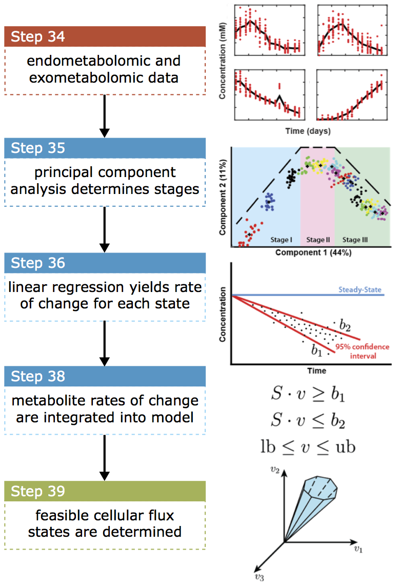
Figure 4: Conceptual overview of the main steps involved in the unsteady-state flux balance analysis (uFBA[87]) method.

The first step is to experimentally quantify the absolute concentrations of a set of extracellular and intracellular metabolites at regular time intervals[87].

35$\leavevmode\nobreak\ |$  Plot the time-course metabolomic data. If the data is non-linear, use principal component analysis to define a sequence of temporal stages during which the time-course metabolomic data can be considered piecewise linear.

36$\leavevmode\nobreak\ |$  Use linear regression to estimate the rate of change of concentration with respect to time for each measured metabolite and for each temporal stage.

37$\leavevmode\nobreak\ |$  Load a standard COBRA
el structure containing the fields
.S,
.b, , ,
ts, and
ns.

38$\leavevmode\nobreak\ |$   Integrate the rate of change in concentration for each measured metabolite with a COBRA model with:

⬇

uFBAoutput = buildUFBAmodel(model, uFBAvariables);

The
Avariables structure must contain the following fields:
tNames is a list of measured metabolites,
angeSlopes provides the rate of change of concentration with respect to time for each measured metabolite,
angeIntervals yields the difference between the mean rate of change of concentration with respect to time and the lower bound of 95% percent confidence interval. The list
oreSlopes contains metabolites whose measurements should be ignored due to insignificant rate of change.

The output is a
Aoutput structure that contains the following fields:
del, a COBRA model structure with constraints on the rate of change of metabolite concentrations,
tsToUse with a list of metabolites with metabolomic data integrated into the model, and
laxedNodes with a list of metabolites that deviate from steady-state along with the direction (i.e., accumulation or depletion) and magnitude (i.e., reaction bound) of deviation. The uFBA algorithm automatically determines sink or demand reactions needed to return a model with at least one feasible flux balance solution, by automatically reconciling potentially incomplete or inaccurate metabolomic data with the model structure. The added sink or demand reactions allow the corresponding metabolites, defined by
laxedNodes, to deviate from a steady state to ensure model feasibility. The default approach is to minimise the number of metabolites that deviate from steady state.

The
ldUFBAmodel function integrates quantitative time course metabolomic data with a model by setting rates of change with respect to time for a set of measured intracellular and extracellular metabolites. A set of sink reactions, demand reactions, or both, may have been added to certain nodes in the network to ensure that the model admits at least one feasible mass balanced flux.

39$\leavevmode\nobreak\ |$   The obtained model can then be minimized using
imizeCbModel:

⬇

model_ufba = optimizeCbModel(uFBAoutput.model);

Integration of transcriptomic and proteomic data  TIMING $10^{2}-10^{4}$ s

40$\leavevmode\nobreak\ |$  Given a generic reconstruction of a biochemical network for a particular organism, some reactions may only be active in a specific tissue, cell-type, or under specific environmental conditions. It is necessary to extract a context-specific model from a generic model in order to create a model that is representative of the part of the biochemical network that is active within a particular context. Each context-specific model is therefore a subset of a generic model. A variety of experimental data can be used to determine the set of reactions that must be part of a context-specific model, including transcriptomic, proteomic, and metabolomic data, as well as complementary experimental data from the literature.

Several model extraction methods have been developed, with different underlying assumptions, and each has been the subject of multiple comparative evaluations[88, 89, 90]. The selection of a model extraction method and its parametrisation, as well as the methods chosen to preprocess and integrate the aforementioned omics data, significantly influences the size, functionality, and accuracy of the resulting context-specific model. Currently, there is insufficient evidence to assert that one model extraction method universally gives the most physiologically accurate models. Therefore, a pragmatic approach is to test the biochemical fidelity of context-specific models generated using a variety of model extraction methods.

The COBRA Toolbox offers six different model extraction methods, accessible via a common interface:

⬇

tissueModel = createTissueSpecificModel(model, options);

The different methods and associated parameters are selected via the
ions structure. The
lver field indicates which method shall be used. The other fields of the
ions structure vary depending on the method and often depend on bioinformatic preprocessing of input omics data. There are additional optional parameters for all algorithms, with the default being the values indicated in the respective papers. Please refer to the original papers reporting each algorithm for details on the requirements for preprocessing of input data. Each of the six different model extraction methods can be invoked using:

1. The TCORE[91] algorithm

   1. One set of core reactions that is guaranteed to be active in the extracted model is identified by TCORE. Then, the algorithm finds the minimum number of reactions possible to support the core;
      re field provides the core reactions which have to be able to carry flux in the resulting model.

2. The ME[92] algorithm

   1. With this algorithm, the usage of low-expression reactions is minimised while keeping the objective (e.g., biomass) above a certain value;
      pressionRxns field provides the reaction expression, with $-1$ for unknown reactions or reactions not linked to genes;
      reshold field sets the threshold above which a reaction is assumed to be active.

3. The T[93] algorithm

   1. T finds the optimal trade-off between including high-expression reactions and removing low-expression reactions;
      pressionRxns field is defined as above;
      reshold_lb field is the threshold below which reactions are assumed to be inactive;
      reshold_ub field is the threshold above which reactions are assumed to be active.

4. The T[94] algorithm

   1. The optimal trade-off between including and removing reactions based on their given weights is determined by this algorithm; ights field provides the weights $w$ for each reaction in the objective of T ($max(\sum_{i\in R}w_{i}y_{i}+\sum_{j\in M}x_{j})$ ). Commonly a high expression leads to higher positive values and low or no detection leads to negative values.

5. The [95] algorithm

   1. defines high-confidence reactions to ensure activity in the extracted model. Medium confidence reactions are only kept when a certain parsimony trade-off is met.
      dium_set field provides the set of reactions that have a medium incidence, while
      gh_set field provides the set of reactions that have to be in the final model. Any reaction not in the medium or high set is assumed to be inactive and preferably not present in the final model.

6. The DRE[96] algorithm

   1. A set of core reactions is first found and all other reactions are then pruned based on their expression, connectivity to core, and confidence score. Reactions that are not necessary to support the core or defined functionalities are thus removed. Core reactions are removed if they are supported by a certain number of zero-expression reactions.
      nfidenceScores field provides reliability for each reaction, generally based on literature, while
      iquityScore field provides the ubiquity score of each reaction in multiple replicates, i.e., the number of times the reaction was detected as active in experimental data under the investigated condition.

CRITICAL STEP When integrating omics data, parameter selection is critical, especially the threshold for binary classification, e.g., the threshold for genes into active or inactive sets. Algorithmic performance often strongly depends on parameter choices and on the choice of data preprocessing method[89]. However,
ateTissueSpecificModel does not offer data preprocessing tools, because the selection of the discretisation method and parameters depend on the origin of the data. However, the COBRA Toolbox offers functionality to map preprocessed expression data to reactions via the function

ExpressionToReactions(model, expression).

Adding biological constraints to a flux balance model   TIMING $\sim 10^{2}$ s

41$\leavevmode\nobreak\ |$  A cell-type or organ-specific model can be converted into a condition-specific model, based on the imposition of experimentally derived constraints. There are several types of constraints that can be imposed on a metabolic network, such as biomass maintenance requirements, environmental constraints, or maximal enzyme activities. In general, biomass constraints[75] are added as part of a biomass reaction. In some instances, however, a cell-type (e.g., neuron) does not divide, but is only required to turn over its biomass components. Turnover rates are commonly expressed as half-lives and represent the time required for half of the biomass precursor to be replaced[97]. A model can be constrained with inequality constraints so as to require a minimal rate of turnover for a metabolite. If that metabolite possesses only one degradation pathway, then it is sufficient to adjust the bounds on a reaction in that pathway. However, if there are multiple possible degradation pathways, then it is necessary to impose a lower bound on the total rates of a set of irreversible degradation reactions, one for each possible degradation pathway of the metabolite in question.

The implementation of such a constraint is illustrated in the following example. In the brain, phosphatidylcholine (PC) can be degraded by three different metabolic pathways[98]:

• Phospholipase D acts on the choline/phosphate bond of PC to form choline and phosphatidic acid (PCHOLP_hs, https://vmh.uni.lu/#reaction/PCHOLP_hs).

• Phospholipase A2 acts on the bond between the fatty acid and the hydroxyl group of PC to form a fatty acid (e.g., arachidonic acid or docosahexaenoic acid) and lysophosphatidylcholine (PLA2_2, https://vmh.uni.lu/#reaction/PLA2_2).

• Ceramide and PC can also be converted to sphingomyelin by sphingomyelin synthetase (SMS, https://vmh.uni.lu/#reaction/SMS).

Load a COBRA model and define the set of reactions that will represent degradation of the metabolite in question:

⬇

multipleRxnList = {'PCHOLP_hs', 'PLA2_2', 'SMS'};

CRITICAL STEP Correctly converting the literature data into bound constraints with the same units used for the model fluxes may be a challenge. Indeed, the curation of biochemical literature to abstract the information required to quantitatively bound turnover rates can take between 4-8 weeks, when the target is to retrieve the biomass composition and the turnover rates of each of the different biomass precursors. Once all the constraints are available, imposing the corresponding reaction bounds takes less than 5 minutes.

42$\leavevmode\nobreak\ |$  Verify that all the reactions are irreversible (the lower and upper bounds should be greater or equal to 0).

⬇

rxnInd = findRxnIDs(model, multipleRxnList);

>> model.lb(rxnInd);

>> model.ub(rxnInd);

43$\leavevmode\nobreak\ |$  Generate and add the constraint:

⬇

c = [1, 1, 1];

>> d = 2.674;

>> ineqSense = 'G';

>> modelConstrained = constrainRxnListAboveBound(model, multipleRxnList, c, d, ineqSense);

where
c is a vector forming the inequality constraint $c^{T}v\geq d$, and
d is a scalar.
qSense encodes the sense of these inequality (
'L' for a lower inequality, or
'G' for an upper inequality). In this example, all entries of $c$ are positive as we seek for the sum of the rates of the three reactions (irreversible in the forward direction) to be greater than $d$. This extra constraint is encoded in the
el.C field.

44$\leavevmode\nobreak\ |$  Check that the constraints are correctly added to the model:

⬇

[nMet, nRxn] = size(modelConstrained.S);

45$\leavevmode\nobreak\ |$  Solve the FBA problem with the extra constraint $c^{T}v\geq d$:

⬇

solution = optimizeCbModel(modelConstrained, 'max', 1e-6);

46$\leavevmode\nobreak\ |$   Check the values of the added fluxes. The sum of fluxes should be greater than or equal to the value of $d$:

⬇

solution.v(rxnInd);

>> sum(c*FBAsolution.v(rxnInd));

Qualitative chemical and biochemical fidelity testing  TIMING $10^{2}-10^{3}$ s

47$\leavevmode\nobreak\ |$   Once a context-specific model is generated, it is highly advisable to frequently compare preliminary model predictions with published experimental data[42]. Such predictions must be compared directly with an unbiased selection of appropriate independent biological literature in order to identify possible sources of misconception or computational misspecification. It is challenging to compare genome-scale predictions with experimental data that may only be available for a subset of a biochemical network. In this context, it is important to first turn to literature relevant to the aspect of the biological network being represented by a model and then check if the literature result is correctly predicted by the model. Inevitably, this is an iterative approach with multiple rounds of iterative refinement of the reconstruction and the model derived from it, before finalising a model version and comparison of final predictions with independent experimental data.

A draft model should be subjected to a range of quantitative and qualitative chemical and biochemical fidelity tests. As described in Step Identify stoichiometrically consistent and inconsistent reactions  TIMING $1-10^{5}s$, chemical fidelity testing includes testing for stoichiometric consistency. This should not be necessary if one starts with a stoichiometrically consistent generic model and extracts a context-specific model from it. However, it is possible that misspecified reactions might have been inadvertently added during refinement of a reconstruction, therefore retest for stoichiometric consistency. Beyond chemical fidelity, it is advised to test again for biochemical fidelity. Such tests are very specific to the particular biological domain that is being modelled. Here we focus on human metabolism and use
elClosed, the
on3Dmodel[77] with all external reactions closed, from Steps Flux balance analysis  TIMING $1-10^{2}$ s-Flux balance analysis  TIMING $1-10^{2}$ s.

It is important to encode and conduct qualitative fidelity tests for anticipated true negatives. The following test is for the production of ATP from water alone in a closed model:

⬇

modelClosedATP = changeObjective(modelClosed, 'DM_atp[c]');

>> modelClosedATP = changeRxnBounds(modelClosedATP, 'DM[atp_c]', 0, 'l');

>> modelClosedATP = changeRxnBounds(modelClosedATP, 'EX_h2o[e]', -1, 'l');

>> FBAsol = optimizeCbModel(modelClosedATP);

If
sol.stat == 0, then the model is incapable of producing ATP from water, as expected. If
sol.stat == 1, then the supposedly closed model can produce ATP from water. This indicates that there are stoichiometrically inconsistent reactions in the network, which need to be identified. See Step Identify stoichiometrically consistent and inconsistent reactions  TIMING $1-10^{5}s$ for instructions how to approach this analysis.

48$\leavevmode\nobreak\ |$  It is also important to encode and conduct qualitative fidelity tests for anticipated true positives. The following metabolic function test is for the production of mitochondrial succinate from 4-Aminobutanoate in a model that is closed to exchange of mass across the boundary of the system, except for the metabolites
'gly[c]', 'co2[c]', and
'nh4[c]'.

⬇

modelClosed = addSinkReactions(modelClosed, {'gly[c]', 'co2[c]', 'nh4[c]'}, ...

[-100, -1; 0.1, 100; 0.1, 100]);

>> modelClosed = changeObjective(modelClosed, 'sink_nh4[c]');

>> sol = optimizeCbModel(modelClosed, 'max', 'zero');

If
sol.stat == 1, then it is feasible for the model to produce mitochondrial succinate from 4-Aminobutanoate. If
sol.stat == 0, then this metabolic function is infeasible. This is not anticipated and indicates that further gap filling is required (see Steps Gap fill a metabolic network  TIMING $10^{2}-10^{5}$ s-Gap fill a metabolic network  TIMING $10^{2}-10^{5}$ s).

Quantitative biochemical fidelity testing  TIMING $10^{2}-10^{3}$ s

49$\leavevmode\nobreak\ |$  It is important to check if a model can reproduce or closely approximate known quantitative features of the biochemical network being represented. Here we illustrate how to predict the ATP yield from different carbon sources under aerobic or anaerobic conditions for Recon3D[77]. These are compared with the values for the corresponding ATP yields obtained from the biochemical literature. This approach can be adapted for condition- and cell-type specific models derived from Recon3D in order to test whether these models are still able to produce physiologically relevant ATP yields. Add and define the ATP hydrolysis reaction
atp[c] to be the objective reaction in the model with:

⬇

modelClosed = addReaction(modelClosed, ...

'DM_atp[c]', 'h2o[c] + atp[c] -> adp[c] + h[c] + pi[c]');

>> modelClosed = changeObjective(modelClosed, 'DM_atp[c]');

50$\leavevmode\nobreak\ |$  Allow the model to uptake oxygen and water, then provide 1 mol/gdw/hr of a carbon source, e.g., glucose (VMH ID:
_D[e]):

⬇

modelClosed.lb(find(ismember(modelClosed.rxns, 'EX_o2[e]'))) = -1000;

>> modelClosed.lb(find(ismember(modelClosed.rxns, 'EX_h2o[e]'))) = -1000;

>> modelClosed.ub(find(ismember(modelClosed.rxns, 'EX_h2o[e]'))) = 1000;

>> modelClosed.ub(find(ismember(modelClosed.rxns, 'EX_co2[e]'))) = 1000;

>> modelClosed.lb(find(ismember(modelClosed.rxns, 'EX_glc_D[e]'))) = -1;

>> modelClosed.ub(find(ismember(modelClosed.rxns, 'EX_glc_D[e]'))) = -1;

51$\leavevmode\nobreak\ |$  Compute a flux balance analysis solution with maximum flux through the
atp[c] reaction:

⬇

FBAsolution = optimizeCbModel(modelClosed, 'max', 'zero');

MinSpan Pathways: a sparse basis of the nullspace of a stoichiometric matrix  TIMING $10^{2}-10^{4}$ s

52$\leavevmode\nobreak\ |$  COBRA models are often mathematically deconstructed into feasible steady state flux vectors in biochemical networks that can be biologically conceptualized as pathways. Much development and analysis has been done for such pathway vectors in terms of elementary flux modes[99], extreme pathways[100], and elementary flux vectors[101]. As the number of elementary or extreme vectors scales exponentially with the size of a typical metabolic network, increasingly efficient algorithms become essential for enumerating elementary or extreme vectors at genome-scale. An alternate approach[102] is to approximately compute a set of $n-\textrm{rank}(S)$ sparse linearly independent flux vectors that together form a basis of the right nullspace of a stoichiometric matrix and also satisfy specified constraints on reaction directionality. This approach requires the solution of a greedy sequence of mixed-integer linear optimisation problems, each of which computes a sparse flux mode that is linearly independent from the rest of the vectors within a nullspace basis. The end result is a sparse set of linearly independent flux modes denoted MinSpan pathways.

Given a model with a stoichiometric matrix, reaction bounds and reaction identifiers, the MinSpan algorithm may be invoked with:

⬇

Z = detMinSpan(model, params);

The
ams structure provides the user ability to change key parameters. Among others, the main parameters include the amount of time
meLimit for each iterative solve in seconds and the number of threads for the MILP solver to use. The output $Z\in\mathbb{R}^{n\times(n-\textrm{rank}(S))}$ is a sparse set of $n-\textrm{rank}(S)$ linearly independent flux modes, each corresponding to a MinSpan pathway.

Low dimensional flux variability analysis  TIMING $1-10^{3}$ s

53$\leavevmode\nobreak\ |$  Flux balance analysis does not, in general, return a unique optimal flux vector. That is, Problem  (1) returns an optimal flux vector, $v^{\star}\in\mathbb{R}^{n}$ with one flux value for each reaction, but typically an infinite set of steady state flux vectors exist that can satisfy the same requirement for an optimal objective, $c^{T}v^{\star}=c^{T}v$, as well as the other equalities and inequalities in Problem (1). Flux variability analysis is a widely used method for evaluating the minimum and maximum range of each reaction flux that can still satisfy the aforementioned constraints using two optimisation problems for each reaction of interest

$$\begin{array}[]{ll}\underset{v}{\textrm{max}\backslash\textrm{min}}&v_{j}\\ \text{s.t.}&Sv=0,\\ &l\leq v\leq u,\\ &c^{T}v=c^{T}v^{\star}.\end{array}$$ (4)

Just as there are many possible variations on flux balance analysis, there are many possible variations on flux variability analysis. The COBRA Toolbox offers a straightforward interface to implement standard flux variability analysis and a wide variety of options to implement variations on flux balance analysis.

1. Standard flux variability analysis

   1. The following command can be invoked to compute standard flux variability analysis:

      ⬇

      [minFlux, maxFlux] = fluxVariability(model);

      The result is a pair of $n$ dimensional column vectors,
      Flux and
      Flux, with the minimum and maximum flux values satisfying Problem (4).

1. Advanced flux variability analysis

   1. The full spectrum of flux variability analysis options can be accessed using the command:

      ⬇

      [minFlux, maxFlux, Vmin, Vmax] = fluxVariability(model, optPercentage, osenseStr, rxnNameList, verbFlag, allowLoops, method);

The
Percentage parameter allows one to choose whether to consider solutions that give at least a certain percentage of the optimal solution. For instance
Percentage = 0 would just find the flux range of each reaction, without of any requirement to satisfy any optimality with respect to flux balance analysis. Setting the parameters
nseStr = 'min' or
nseStr = 'max' determines whether the flux balance analysis problem is first solved as a minimisation or maximisation. The
NameList accepts a cell array list of reactions to selectively perform flux variability upon. This is useful for high dimensional models, for which the computation of a flux variability for all reactions is more time consuming. The additional $n\times k$ output matrices
n and
x return the flux vector for each of the $k\leq n$ fluxes selected for flux variability. The
bFlag input determines how much output shall be printed. The parameter
owLoops == 0 invokes a mixed integer linear programming implementation of thermodynamically constrained flux variability analysis for each minimisation or maximisation of a reaction rate. The
hod input argument determines whether the output flux vectors also minimise the
orm,
orm or
orm while maximising or minimising the flux through one reaction.

The default result is a pair of maximum and minimum flux values for every reaction. Optional parameters may be set. For instance, parameters can be set to control which subset of $k\leq n$ reactions of interest that shall be be obtained, or to determine the characteristics of each of the $2\times k$ flux vectors.

High dimensional flux variability analysis  TIMING $1-10^{5}$ s

54$\leavevmode\nobreak\ |$   Besides flux balance analysis, flux variability analysis is the most widely used constraint-based modelling method for high-dimensional models. However, its use in this setting requires a more sophisticated computational approach, with a multi-core processor[103], or computational cluster[53], and a commercial-grade linear optimisation solver. In this setting, advanced users have two options:

1. Use
   tFVA with MATLAB

   1. Solve the $2\times k$ linear optimisation problems using multiple threads running on parallel processors with
      tFVA, which depends on the CPLEX solver (IBM Inc.), using the command :

      ⬇

      [minFlux, maxFlux, optsol] = fastFVA(model, optPercentage, osenseStr);

      The output argument
      sol returns the optimal solution of the initial FBA.

2. Use distributedFBA.jl with Julia

   1. An alternative is to solve the $2\times k$ linear optimisation problems using multiple threads running on parallel processors or a cluster using distributedFBA.jl, an openCOBRA extension that permits the solution of flux balance analysis, a distributed set of flux balance problems, or a flux variability analysis using a common of solver (GLPK, CPLEX, Clp, Gurobi, Mosek). Assuming that distributedFBA.jl has been correctly installed and configured, the commands to go back and forth between a model or results in MATLAB and the computations in Julia are:

      ⬇

      save('high_dimensional_model.mat', unimodel);

      ⬇

      # -- switch to Julia --

      julia> model = loadModel("high_dimensional_model.mat");

      julia> workersPool, nWorkers = createPool(128);

      julia> minFlux, maxFlux, optSol, fbaSol, fvamin, fvamax = distributedFBA(model, solver, nWorkers=nWorkers, optPercentage=optPercentage, preFBA=true);

      julia> saveDistributedFBA("high_dimensional_FVA_results.mat");

      # -- switch to MATLAB --

      ⬇

      load('high_dimensional_FVA_results.mat');

      Here,
      rkers = 128 will distribute the flux variability analysis problem amongst 128 Julia processes on one or more computing nodes in a computational cluster.

Uniform sampling of steady-state fluxes   TIMING $1-10^{3}$ s

55$\leavevmode\nobreak\ |$  An unbiased characterisation of the set of flux vectors consistent with steady state, mass balance, and reaction bound constraints can be obtained by uniformly sampling the feasible set
$\Omega\coloneqq\left\{v\mid Sv=0;\leavevmode\nobreak\ l\leq v\leq u\right\}$. The feasible set for sampling should be defined based on biochemically justifiable constraints. These are the same conditions that apply when formulating the flux balance analysis Problem (1), except that there is no need to formulate a linear objective. To ensure the sample is statistically representative of the entire feasible set, a sufficiently large number of flux vectors and the flux vectors must be collected randomly within the feasible set. Recently, we distributed new software to uniformly sample feasible sets of steady state fluxes[104] based on a coordinate hit-and-run with rounding (CHRR) algorithm[105, 106] that is guaranteed to return a statistically uniform distribution when appropriately utilised. The CHRR sampling algorithm is therefore used by default. Figure 5 illustrates the basics of this algorithm.

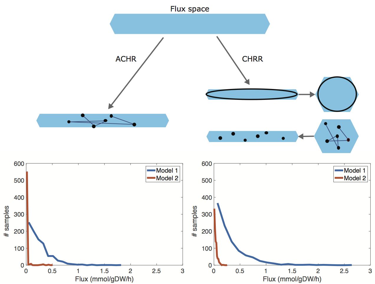
Figure 5: Solution spaces from steady state fluxes are anisotropic, that is, long in some directions and short in others. This impedes the ability of any sampling algorithm taking a random direction to evenly explore the full feasible set (artificial centering hit-and-run (ACHR) algorithm). The CHRR (coordinate hit-and-run with rounding) algorithm first rounds the solution space based on the maximum volume ellipsoid. Then, the rounded solution space is uniformly sampled using a provably efficient coordinate hit-and-run random walk. Finally, the samples are projected back onto the anisotropic feasible set. This leads to a more distributed uniform sampling, so that the converged sampling distributions for the selected reactions become smoother. As an example, for both sampling distributions, the parameters were defined as: $nSkip=8\times(dim(fluxSpace))^{2}$, $nSamples=1000$.

Sampling of a model is invoked either by using the default setting or by tailoring the parameters with more arguments to the interface. A pragmatic approach is to first try Option (A) with the default parameters, then check the quality of the marginal flux distribution for a subset of reactions (see Figure 5). Especially for higher dimensional models, it may be necessary to tune the parameters with Option (B).

1. Sampling of a mono-scale model with $\lesssim\leavevmode\nobreak\$2000 variables

   1. A Model that contains less than 2000 variables can usually be sampled using the default settings:

      ⬇

      [modelSampling, samples] = sampleCbModel(model);

      The
      ples output is an $n\times p$ matrix of sampled flux vectors, where $p$ is the number of samples. In order to accelerate any future rounds of sampling, use the
      elSampling output. This is a model storing extra variables acquired from preprocessing the model for sampling (see Figure 5).

2. Sampling of a model with $\lesssim\leavevmode\nobreak\$10000 variables

   1. Larger Models containing less than 10000 variables may be sampled by tuning the optional input parameters:

      ⬇

      [modelSampling, samples] = sampleCbModel(model, sampleFile, samplerName, options, ...

      modelSampling);

      The variable
      pleFile contains the name of a .mat file used to save the sample vectors to disk. A string passed to
      plerName can be used to sample with non-default solvers. The
      ions structure contains fields that control the sampling density (
      kip) and the number of samples (
      amples). The total number of
      ples returned is $p=nSkip\;\times\;nSamples$. The output
      elSampling may be used in subsequent rounds of sampling. Although rounding large models is computationally demanding, the results can be reused when sampling the same model more than once. The CHRR algorithm provably converges to a uniform stationary sampling distribution if enough samples are obtained and has been tested with mono-scale metabolic models with up to $10000$ reactions. The default parameters are set using heuristic rules to estimate a sufficiently large number of samples, which balances this requirement against the desire to complete the sampling procedure in a practically useful period of time.  ? TROUBLESHOOTING

Identify all genetic manipulations leading to targeted overproductions   TIMING $10-10^{5}\leavevmode\nobreak\$s

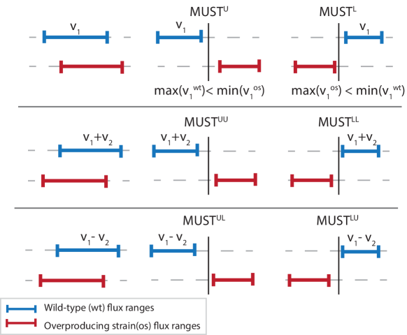
Figure 6: In the OptForce procedure, the MUST sets are determined by contrasting the flux ranges obtained using flux variability analysis (FVA) of a wild-type (blue bars) and an overproducing strain (red bars). The first order MUST sets (top panel) are denoted MUST${}^{\textrm{L}}$ and MUST${}^{\textrm{U}}$. For instance, a reaction belongs to the MUST${}^{\textrm{U}}$ set if the upper bound of the flux range in the wild-type is less than the lower bound of the flux range of the overproducing strain. The center and bottom panels show all possible second order MUST sets.

56$\leavevmode\nobreak\ |$   A variety of strain design algorithms[69] are implemented within the COBRA Toolbox, including OptKnock[107], OptGene[108], Genetic Design Local Search (GDLS[109]), and OptForce[110]. While OptKnock, OptGene, and GDLS could identify gene deletion strategies, the OptForce method can identify not only gene deletion but also up- and down-regulation strategies. As the OptForce method is new to this version of the COBRA Toolbox, we provide an illustrative example of strain design using this method.

Consider the problem of finding a set of interventions of size
K such that when these interventions are applied to a wild-type strain, the mutant created will produce a particular target of interest at a higher yield than the wild-type strain. The interventions could be knock-outs (zero out the flux for a particular reaction), up-regulations (increase the flux for a particular reaction), or down-regulations (decrease the flux for a particular reaction). As an example, we will use the OptForce method to identify all genetic manipulations leading to the overproduction of succinate in E. coli[110]. The OptForce method consists of the following set of steps: define the constraints for both wild-type and mutant strains, perform flux variability analyses for both wild-type and mutant strains, find the sets of reactions that must alter their flux in order to achieve the desired phenotype in the mutant strain, and, finally, find the interventions needed to ensure an increased production of the target of interest (Steps 6-6).

First, select a commercial-grade solver and select the local directory to save the generated results with:

⬇

changeCobraSolver('gurobi', 'ALL');

57$\leavevmode\nobreak\ |$  Load an illustrative model that comprises only $90$ reactions, describing the central metabolism in E. coli[111].

⬇

readCbModel('AntCore.mat');

58$\leavevmode\nobreak\ |$  Set the objective function to maximise the biomass reaction (). Change the lower bounds such that E. coli model will be able to consume glucose, oxygen, sulfate, ammonium, citrate, and glycerol.

⬇

model = changeObjective(model, 'R75', 1);

>> for rxn = {'EX_gluc', 'EX_o2', 'EX_so4', 'EX_nh3', 'EX_cit', 'EX_glyc'}

model = changeRxnBounds(model, rxn, -100, 'l');

end

59$\leavevmode\nobreak\ |$  Define the constraints for both wild-type and mutant strains:

⬇

constrWT = struct('rxnList', {{'R75'}}, 'rxnValues', 14, 'rxnBoundType', 'b');

>> constrMT = struct('rxnList', {{'R75', 'EX_suc'}}, 'rxnValues', [0, 155.55], ...

'rxnBoundType', 'bb');

CRITICAL STEP In this example, we provide the constraints for both wild-type and mutant strains, but in a typical scenario the definition of differential constraints on wild-type and mutant strains requires additional research. This step could take a few days or weeks, depending on the information available for the species of interest. Flux bounds (i.e., uptake rate and minimum biomass yield target) are required inputs. New experiments might be required to be performed in addition to the literature curation task in order to obtain such data. Assumptions may also be made when describing the phenotypes of both strains, which will reduce the dependency on literature curation. It is important that the two strains are sufficiently different in order to be able to anticipate differences in reaction ranges.

60$\leavevmode\nobreak\ |$  Performing flux variability analysis for both wild-type and mutant strains with:

⬇

[minFluxesW, maxFluxesW, minFluxesM, maxFluxesM] = FVAoptForce(model, constrWT, constrMT);

>> disp([minFluxesW, maxFluxesW, minFluxesM, maxFluxesM]);

61$\leavevmode\nobreak\ |$  The MUST sets are the sets of reactions that must increase or decrease their flux in order to achieve the desired phenotype in the mutant strain. As shown in Figure 6, the first order MUST sets are
tU and
tL while second order MUST sets are denoted as
tUU,
tLL, and
tUL. After parameters and constraints are defined, the functions
dMustL and
dMustU are run to determine the
tU and
tL sets, respectively. Define an ID of the run with:

⬇

runID = 'TestoptForceM';

Each time the MUST sets are determined, folders are generated to read inputs and store outputs, i.e., reports. These folders are located in the directory defined by the uniquely defined
ID.

62$\leavevmode\nobreak\ |$  In order to find the first order MUST sets, constraints should be defined:

⬇

constrOpt = struct('rxnList', {{'EX_gluc', 'R75', 'EX_suc'}}, 'values', [-100; 0; 155.5]);

63$\leavevmode\nobreak\ |$  The first order MUST set
tL is determined by running:

⬇

[mustLSet, pos_mustL] = findMustL(model, minFluxesW, maxFluxesW, ...

'constrOpt', constrOpt, 'runID', runID);

If
ID is set to
'TestoptForceL', a folder TestoptForceL is created, in which two additional folders InputsMustL and OutputsMustL are created. The InputsMustL folder contains all the inputs required to run the function
dMustL, while the OutputsMustL folder contains the
tL set found and a report that summarises all the inputs and outputs. In order to maintain a chronological order of computational experiments, the report is timestamped.

64$\leavevmode\nobreak\ |$  Display the reactions that belong to the
tL set using:

⬇

disp(mustLSet)

65$\leavevmode\nobreak\ |$  The first order MUST set
tU is determined by running:

⬇

[mustUSet, pos_mustU] = findMustU(model, minFluxesW, maxFluxesW, ...

'constrOpt', constrOpt, 'runID', runID);

The results are stored and available in a format analogous to the
tL set. The reactions that belong to the
tU may be displayed in the same way as
tL.

66$\leavevmode\nobreak\ |$  Define the reactions that will be excluded from the analysis. The reactions found in the previous step as well as exchange reactions shall be included.

⬇

constrOpt = struct('rxnList', {{'EX_gluc', 'R75', 'EX_suc'}}, 'values', [-100, 0, 155.5]');

>> exchangeRxns = model.rxns(cellfun(@isempty, strfind(model.rxns, 'EX_')) == 0);

>> excludedRxns = unique([mustUSet; mustLSet; exchangeRxns]);

67$\leavevmode\nobreak\ |$  The second order MUST set
tUU can be determined by running:

⬇

[mustUU, pos_mustUU, mustUU_linear, pos_mustUU_linear] = findMustUU(model, minFluxesW, ...

maxFluxesW, 'constrOpt', constrOpt, ...

'excludedRxns', excludedRxns,'runID', runID);

The results are stored and available in a format analogous to the
tL set. The reactions of the
tUU can be displayed using the
p function.

68$\leavevmode\nobreak\ |$  Repeat the above steps to determine the second order MUST sets
tLL and
tUL by using the functions
dMustLL and
dMustUL respectively. The results are stored and available in a format analogous to the
tL set. In the present example,
tLL and
tUL are empty sets. ? TROUBLESHOOTING

69$\leavevmode\nobreak\ |$  In order to find the interventions needed to ensure an increased production of the target of interest, define the
tU set as the union of the reactions that must be up-regulated in the first and second order MUST sets. Similarly,
tL may be defined.

⬇

mustU = unique(union(mustUSet, mustUU));

>> mustL = unique(union(mustLSet, mustLL));

70$\leavevmode\nobreak\ |$  Define the number of interventions
k allowed, the maximum number of sets to find
ts, the reaction producing the metabolite of interest
getRxn (in this case, succinate), and the constraints on the mutant strain
strOpt.

⬇

k = 1; nSets = 1; targetRxn = 'EX_suc';

>> constrOpt = struct('rxnList', {{'EX_gluc','R75'}}, 'values', [-100, 0]);

71$\leavevmode\nobreak\ |$  Run the OptForce algorithm and display the reactions identified by
Force with:

⬇

[optForceSets, posoptForceSets, typeRegoptForceSets, flux_optForceSets] = optForce(model, targetRxn, mustU, mustL, minFluxesW, maxFluxesW, minFluxesM, maxFluxesM, 'k', k, 'nSets', nSets, 'constrOpt', constrOpt, 'runID', runID);

>> disp(optForceSets)

72$\leavevmode\nobreak\ |$  In order to find non-intuitive solutions, increase the number of interventions
k and exclude the
t reaction from up-regulations. Increase
ts to find the $20$ best sets. Change the
ID to save this second result in a separate folder from the previous result, then run
Force again as in Step 6.

⬇

k = 2; nSets = 20; runID = 'TestoptForceM2';

>> excludedRxns = struct('rxnList', {{'SUCt'}}, 'typeReg','U');

73$\leavevmode\nobreak\ |$  The reactions determined by
Force can be displayed using
p(optForceSets). The complete set of predicted interventions can be found in the folders created inside the
ID folder in which inputs and outputs of
Force and associated
dMust* functions are stored. The input folders InputsFindMust* contain .mat files for running the functions to solve each one of the bilevel optimisation problems. The output folders OutputsFindMust* contain results of the algorithms (saved as .xls and .txt files) as well as a report (a .txt file) that summarises the outcome of the steps performed during the execution of each function. The
Force algorithm will find sets of reactions that should increase the production of a specified target. The first sets found should be the best ones because the production rate will be the highest. The last ones will be the worst, as the production rate is the lowest. ! CAUTION Be aware that some sets may not guarantee a minimum production rate for a target, so check the minimum production rate, e.g., using the function
toptForceSol.

Atomically resolve a metabolic reconstruction  TIMING $10-10^{5}$ s

74$\leavevmode\nobreak\ |$  In most genome-scale metabolic models, it is not explicit that the stoichiometric matrix represents a network of biochemical reactions. It is implicit that each row of the stoichiometric matrix corresponds to some molecular species, but when computing properties of the model, the atomic structure of each molecular species is not represented. It is also implicit that each column of the stoichiometric matrix corresponds to some biochemical reaction. However, when computing properties of the model, the mechanisms of the underlying biochemical reaction, in terms of the structures of the metabolites and the atomically resolved chemical transformations that take place, are not represented. Recent developments in genome-scale metabolic modelling have generated genome-scale metabolic reconstructions where the molecular structures are specified[112] and the reaction mechanisms are represented by atom mappings between substrate and product atoms[113, 77].

An atom mapping is a one-to-one association between a substrate atom and a product atom. An instance of a chemical reaction may be represented by a set of atom mappings, with one atom mapping between each substrate and product atom. A single chemical reaction can admit multiple chemically equivalent atom mappings when chemically equivalent atoms are present in a substrate, a product, or both. Therefore, each chemical reaction may be represented by one set, or multiple chemically equivalent sets, of atom mappings. Together, a set of atom mappings for a chemical reaction specify key aspects of the reaction mechanism, e.g., chemical bond change, breakage, and formation. The Virtual Metabolic Human database (VMH, http://vmh.life) provides metabolites chemical structures and atom mapped reactions for $9,610$ reactions in Recon3D[77] and $4,831$ metabolites from Recon3D[77] and the human gut microbiota[1]. Metabolite structures are provided in canonically ordered MOL and SMILES formats. Atom mapping data are provided in both RXN and SMILES formats. This explicit representation of metabolite and reaction structure offers the possibility of a broader range of biological, biomedical and biotechnological applications than with stoichiometry alone.

In order to obtain chemical structures for each metabolite, there are three main ways:

1. Use chemoinformatics software tools

   1. Suitable cheminformatics software tools[112] may be used to automatically obtain metabolite identifiers in metabolic network reconstructions and download the corresponding structure from a database.

2. Manually interrogate metabolic databases

   1. Databases such as VMH (http://vmh.life), PubChem[114], KEGG[115], ChEBI[116], LMSD[117], BioPath database[118], ChemSpider database[119], HMDB[120], etc provide chemical structures for metabolites in a network.

3. Manually draw structures of metabolites

   1. Based on chemical knowledge, one could manually draw structures of metabolites using tools such as ChemDraw (PerkinElmer, https://perkinelmer.com/ChemDraw).

75$\leavevmode\nobreak\ |$  In order to obtain an atom mapping for a metabolic reaction, the reaction stoichiometry and the chemical structures of the corresponding metabolites must be available. To obtain atom mappings, there are three main options:

1. Use software tools for prediction of atom mappings

   1. A comparative study has been performed using Recon3D as a test case[113]. Due to its accuracy and availability, Reaction Decoder Tool (RDT[122]) is considered being the most suitable algorithm to atom map the reactions from a genome-scale metabolic network. Nevertheless, note that the Canonical Labelling for Clique Approximation (CLCA[123]) algorithm can map reactions with explicit hydrogen atoms for fully protonated reactions, while RDT can only atom map reactions with implicit hydrogen atoms.

2. Manually interrogate metabolic databases

   1. Databases such as BioPath[118] and KEGG RPAIR[121] disseminate manually curated atom mappings. VMH (http://vmh.life) also contains manually curated atom mappings for a subset of human metabolic reactions.

3. Manually draw atom mappings

   1. Based on chemical knowledge, one could draw atom mappings using tools such as ChemDraw (PerkinElmer, https://perkinelmer.com/ChemDraw).

76$\leavevmode\nobreak\ |$   Given a
el structure and the directory containing the chemical structure files (
FileDir) in MDL MOL file format, RDT can be invoked to atom map a metabolic model using:

⬇

balancedRxns = obtainAtomMappingsRDT(model, molFileDir, outputDir, ...

maxTime, standardiseRxn);

This function computes atom mapping data for the balanced and unbalanced reactions in the metabolic network and saves it in the
putDir directory. The optional
Time parameter sets a runtime limit for atom mapping of a reaction. If
ndardiseRxn == 1, then atom mappings are also canonicalised, which is necessary in order to obtain a consistent interoperable set of atom mappings for certain applications, e.g., computation of conserved moieties in Step Atomically resolve a metabolic reconstruction  TIMING $10-10^{5}$ s. The output
ancedRxns contains the balanced atom mapped metabolic reactions. ? TROUBLESHOOTING

77$\leavevmode\nobreak\ |$   With a set of canonicalised atom mappings for a metabolic network, the set of linearly independent conserved moieties for a metabolic network can be identified[124]. Each of these conserved moieties corresponds to a molecular substructure (set of atoms in a subset of a molecule) whose structure remains invariant despite all the chemical transformations in a given network. A conserved moiety is a group of atoms that follow identical paths through metabolites in a metabolic network. Similarly to a vector in the (right) nullspace of a stoichiometric matrix that corresponds to a pathway (see Step MinSpan Pathways: a sparse basis of the nullspace of a stoichiometric matrix  TIMING $10^{2}-10^{4}$ s), a conserved moiety corresponds to a vector in the left nullspace of a stoichiometric matrix. Metabolic networks are hypergraphs[125], while most moiety subnetwork are graphs. Therefore conserved moieties have both biochemical and mathematical significance and once computed, can be used for a wide variety of applications. Given a metabolic network of exclusively mass balanced reactions, one can identify conserved moieties by a graph theory analysis of its atom transition network[124].

First compute an atom transition network for a metabolic network using:

⬇

ATN = buildAtomTransitionNetwork(model, rxnfileDir);

where
fileDir is a directory containing only atom mapped files from balanced reactions, which can be obtained as explained in Step Atomically resolve a metabolic reconstruction  TIMING $10-10^{5}$ s. The output is a structure with several fields:
.A is a $p\times q$ sparse incidence matrix for the atom transition network, where $p$ is the number of atoms and $q$ is the number of atom transitions,
ts is a $p\times 1$ cell array of metabolite identifiers to link each atoms to its corresponding metabolites,
ns is a $q\times 1$ cell array of reaction identifiers to link atom transitions to their corresponding reactions, and
ements is a $p\times 1$ cell array of element symbols for atoms in
.A.

CRITICAL STEP All the RXN files needed to compute the atom transition network must be in a canonical format. This can be achieved by setting
ndardiseRxn = 1.

78$\leavevmode\nobreak\ |$  In order to identify the conserved moieties in the metabolic network, invoke:

⬇

[L, M, moietyFormulas] = identifyConservedMoieties(model, ATN);

where
L represents the conserved moieties in the metabolic network. That is,
L is an $m\times r$ matrix of $r$ moiety vectors in the left null space of the stoichiometric matrix,
M is the $u\times v$ incidence matrix of the moiety supergraph in which each connected component is a moiety graph, and
etyFormulas is an $m\times r$ cell array with chemical formulas of the computed moieties.

Thermodynamically constrain a metabolic model  TIMING $1-10^{3}$ s

79$\leavevmode\nobreak\ |$  In flux balance analysis of genome-scale stoichiometric models of metabolism, the principal constraints are uptake or secretion rates, the steady state mass conservation assumption, and reaction directionality. The COBRA Toolbox extension vonBertalanffy[126] is a set of methods for integration of thermochemical data with constraint-based models[49, 127, 128] as well as application of thermodynamic laws to increase the physicochemical fidelity of constraint-based modelling predictions[129]. A full exposition of the method to thermodynamically constrain a genome-scale metabolic model is beyond the scope of this protocol. Therefore, only several key steps are highlighted.

Given a set of experimentally derived
ining_data on standard transformed Gibbs energies of formation, a state-of-the art quantitative estimation of standard Gibbs energy of formation for metabolites with similar chemical substructures can be obtained using an implementation of the component contribution method[128]. We assume that the input
el has been anatomically resolved as described in Steps Atomically resolve a metabolic reconstruction  TIMING $10-10^{5}$ s-Atomically resolve a metabolic reconstruction  TIMING $10-10^{5}$ s. Access to a compendium of stoichiometrically consistent metabolite structures[112, 124] is a prerequisite. The component contribution method is then invoked as follows:

⬇

model = componentContribution(model, training_data);

The
el.DfG0 field gives the estimated standard Gibbs energy of formation for each metabolite in the model with
el.DfG0_Uncertainty field expressing the uncertainty in these estimates, which is smaller for metabolites structurally related to metabolites in the training set. All thermodynamic estimates are given in units of kJ/mol.

80$\leavevmode\nobreak\ |$  The standard Gibbs energy of formation for each metabolite must be transformed according to the environment of each compartment of the model[127], i.e., the temperature, pH, ionic strength and electrical potential specific to each compartment. Then the thermodynamic properties of reactions are estimated, given
el.concMin and
el.concMax where one can supply lower and upper bounds on compartment-specific metabolite concentrations (mol/L), which may be achieved with:

⬇

model = setupThermoModel(model, confidenceLevel);

In the output, field
Gt0 of
el gives the estimated standard transformed Gibbs energy of formation for each metabolite and
Gt0 gives the estimated standard transformed Gibbs energy for each reaction. Subject to a
fidenceLevel specified as an input, the upper and lower bounds on standard transformed Gibbs energy for each reaction are provided in
GtMin and
GtMax respectively.

CRITICAL STEP In a multi-compartmental model, this step must be done for an entire network at once in order to ensure that thermodynamic potential differences, arising from differences in the environment between compartments, are properly taken into account. See[127] for a theoretical justification for this assertion.

81$\leavevmode\nobreak\ |$  Reaction directionality may be quantitatively assigned based on the aforementioned thermodynamic estimates with:

⬇

[modelThermo, directions]= thermoConstrainFluxBounds(model, confidenceLevel, DrGt0_Uncertainty_Cutoff);

If
el.DrGtMax(j) < 0, then the $j^{th}$ reaction is assigned to be forward, and if
el.DrGtMin(j) > 0 then the $j^{th}$ reaction is assigned to be reverse, unless the uncertainty in estimation of standard transformed reaction Gibbs energy exceeds a specified cutoff (
t0_Uncertainty_Cutoff). In this case, the qualitatively assigned reaction directionality, specified together by
el.lb(j) and
el.ub(j), takes precedence. The
ections output provides a set of boolean vector fields that can be used to analyse the effect of qualitatively versus quantitatively assigning reaction directionality using thermochemical parameters.

82$\leavevmode\nobreak\ |$  Thermodynamically constrained flux balance analysis may then be invoked by disallowing flux around stoichiometrically balanced cycles, also known as loops, using the
owLoops parameter to
imizeCbModel with:

⬇

allowLoops = 0;

>> solution = optimizeCbModel(model, [], [], allowLoops);

The
ution structure is the same as for flux balance analysis (see Problem (1)), except that this
ution satisfies additional constraints that ensure the predicted steady state flux vector is thermodynamically feasible[130]. The solution satisfies energy conservation and the second law of thermodynamics[131].

Convert a flux balance model into a kinetic model   TIMING $1-10^{3}$ s

83$\leavevmode\nobreak\ |$  In order to analyse biochemical networks at genome scale, systems biologists often use a linear optimisation technique called flux balance analysis (FBA). Linear approximation to known nonlinear biochemical reaction network function is sufficient to get biologically meaningful predictions in some situations. However, there are many biochemical processes where a linear approximation is insufficient, which motivates the quest for developing variational kinetic modelling[132, 133, 134]. Certain conditions are required to be met in order to generate a kinetic model that is internally consistent. First we describe those conditions, then we demonstrate how to ensure that they are met. Consider a biochemical network with $m$ molecular species and $n$ reversible reactions. We define forward and reverse stoichiometric matrices, $F,R\in\mathbb{\mathbb{Z}}_{+}^{m\times n}$, respectively, where $F_{ij}$ denotes the stoichiometry of the $i^{th}$ molecular species in the $j^{th}$ forward reaction and $R_{ij}$ denotes the stoichiometry of the $i^{th}$ molecular species in the $j^{th}$ reverse reaction. We assume that the network of reactions is stoichiometrically consistent[73], that is, there exists at least one positive vector $l\in\mathbb{R}_{++}^{m}$ satisfying $(R-F)^{T}l=0$. Equivalently, we require that every reaction conserves mass. The matrix $N:=R-F$ represents net reaction stoichiometry and may be viewed as the incidence matrix of a directed hypergraph[125]. We assume that there are less molecular species than there are net reactions, that is $m<n$. We assume the cardinality of each row of $F$ and $R$ is at least one, and the cardinality of each column of $R-F$ is at least two. The matrices $F$ and $R$ are sparse and the particular sparsity pattern depends on the particular biochemical network being modelled. Moreover, we assume that $\text{rank}([F,R])=m$, which is a requirement for kinetic consistency[48].

Compute a non-equilibrium kinetic steady state   TIMING $1-10^{3}$ s

84$\leavevmode\nobreak\ |$  Let $c\in\mathbb{R}_{++}^{m}$ denote a variable vector of molecular species concentrations. Assuming constant nonnegative elementary kinetic parameters $k_{f},k_{r}\in\mathbb{R}_{+}^{n}$, we assume elementary reaction kinetics for forward and reverse elementary reaction rates as $s(k_{f},c):=\exp(\ln(k_{f})+F^{T}\ln(c))$ and $r(k_{r},c):=\exp(\ln(k_{r})+R^{T}\ln(c))$, respectively, where $\exp(\cdot)$ and $\ln(\cdot)$ denote the respective component-wise functions[135, 48]. Then, the deterministic dynamical equation for time evolution of molecular species concentration is given by

$$\frac{dc}{dt} \equiv N(s(k_{f},c)-r(k_{r},c))$$

$$= N\left(\exp(\ln(k_{f})+F^{T}\ln(c)\right)-\exp\left(\ln(k_{r})+R^{T}\ln(c))\right)=:-f(c).$$

A vector $c^{*}$ is a steady state if and only if it satisfies $f(c^{*})=0,$ leading to the nonlinear system

$$f(x)=0.$$

There are many algorithms that can handle this nonlinear system by minimising a nonlinear least-squares problem; however, particular features of this mapping, such as sparsity of stoichiometric matrices $F$ and $R$ and non-unique local zeros of mapping $f$, motivates the quest for developing several algorithms for efficient dealing with this nonlinear system. A particular class of such mappings, called duplomonotone mapping, was studied for biochemical networks[136] and three derivative-free algorithms for finding zeros of strongly duplomonotone mappings were introduced. Further, it is shown that the function $\|f\left(x\right)\|^{2}$ can be rewritten as a difference of two convex functions that is suitable to be minimised with DC programming methods[135]. Therefore, a DC algorithm and its acceleration with adding a line search technique were proposed for finding a stationary point of $\|f\left(x\right)\|^{2}$. Since the mapping $f$ has locally non-unique solutions, it does not satisfy classical assumptions (e.g., nonsingularity of the Jacobian) for convergence theory. As a result, it was proved that the mapping satisfies the so-called Hölder metric subregularity assumption[137] and an adaptive Levenberg-Marquardt method was proposed to find a solution of this nonlinear system if the starting point is close enough to a solution. In order to guarantee the convergence of the Levenberg-Marquardt method with arbitrary starting point, it is combined with globalisation techniques such as line search or trust-region, which leads to computationally efficient algorithms.

Compute a non-equilibirum kinetic steady state by running the function
imizeVKmodels. The mandatory inputs for computing steady states are a model
odel containing $F$ and $R$, the name of a solver to solve the nonlinear system, an initial point
x0, and parameters for the considered solvers. For example, for specifying a solver, we write
ver = 'LMTR';. Optional parameters for the selected algorithm may be given to
imizeVKmodels by the
ams struct as follows

⬇

params.MaxNumIter = 1000; params.adaptive = 1; params.kin = kin;

Otherwise, the selected algorithm will be run with the default parameters assigned for each algorithm. Running the function
imizeVKmodels is done by typing

⬇

output = optimizeVKmodels(vKModel, solver, x0, params);

The
put struct contains information related to the execution of the solver.

Compute a moiety conserved non-equilibrium kinetic steady state   TIMING $1-10^{3}$ s

85$\leavevmode\nobreak\ |$  Let us note that a vector $c^{*}$ is a steady state of the biochemical system if and only if

$$s(k_{f},c^{*})-r(k_{r},c^{*})\in\mathcal{N}(N),$$

where $\mathcal{N}(N)$ denotes the null space of $N$. Therefore, the set of steady states $\Omega=\left\{c\in\mathbb{R}_{++}^{m}|\,f(c)=0\right\}$ is unchanged if the matrix $N$ is replaced by a matrix $\bar{N}$ with the same kernel. Suppose that $\bar{N}\in\mathbb{Z}^{r\times n}$ is the submatrix of $N$ whose rows are linearly independent; then $\mathrm{rank}\left(\bar{N}\right)=\mathrm{rank}(N)\eqqcolon r.$ If one replaces $N$ by $\bar{N}$ and transforms (Compute a non-equilibrium kinetic steady state   TIMING $1-10^{3}$ s) to logarithmic scale, and by letting $x\coloneqq\ln(c)\in\mathbb{R}^{m}$, $k\coloneqq[\ln(k_{f})^{T},\,\ln(k_{r})^{T}]^{T}\in\mathbb{R}^{2n}$, then the right-hand side of (Compute a non-equilibrium kinetic steady state   TIMING $1-10^{3}$ s) is equal to the function

$$\bar{f}(x):=\left[\bar{N},-\bar{N}\right]\exp\left(k+[F,\,R]^{T}x\right),$$ (6)

where $\left[\,\cdot\thinspace,\cdot\,\right]$ stands for the horizontal concatenation operator. Let $L\in\mathbb{R}^{m-r,m}$ denote a basis for the left nullspace of $N$, which implies $LN=0$. We have $\mathrm{rank}(L)=m-r$. We say that the system satisfies moiety conservation if for any initial concentration $c_{0}\in\mathbb{R}_{++}^{m}$,

$$L\,c=L\,\mathrm{exp}(x)=l_{0},$$

where $l_{0}\in\mathbb{R}_{++}^{m}.$ It is possible to compute $L$ such that each corresponds to a structurally identifiable conserved moiety in a biochemical network[124]. The problem of finding the moiety conserved steady state of a biochemical reaction network is equivalent to solving the nonlinear system of equations

$$h(x):=\left(\begin{array}[]{c}\bar{f}(x)\\ L\,\mbox{exp}(x)-l_{0}\end{array}\right)=0.$$ (7)

Among algorithms mentioned in the previous section, the local and global Levenberg-Marquardt methods[137] are designed to compute either a solution of the nonlinear system (7) or a stationary point of the merit function $\frac{1}{2}\|h\left(x\right)\|^{2}$. The computation of a moiety conserved non-equilibrium kinetic steady state is made by running the
imizeVKmodels function in the same way as in previous section. A model
odel containing $F$ and $R$, $L$ and $l_{0}$ is then passed to
imizeVKmodels together with the name of one of the Levenberg-Marquardt solvers.

Human metabolic network visualisation with ReconMap  TIMING $1-10^{2}$ s

86$\leavevmode\nobreak\ |$  The visualisation of biochemical pathways is an important tool for biologically interpreting predictions generated by constraint-based models. It can be an invaluable aid for developing an understanding of the biological meaning implied by a prediction. Biochemical network maps permit the visual integration of model predictions with the underlying biochemical context. Patterns that are very difficult to appreciate in a vector can often be much better appreciated by studying a generic map contextualised with model predictions. Genome-scale biochemical network visualisation is particularly demanding. No currently available software satisfies all of the requirements that might be desired for visualisation of predictions from genome-scale models. Automatic layout of genome-scale biochemical networks is insufficiently developed to generate an aesthetically pleasing map, yet manual layout of such maps is very labour intensive and there is no global reference coordinate system for such maps, so each human might layout a global map differently. Software applications for graph visualisation are often not suited to displaying metabolic hypergraphs[138]. Client-server software models have to trade off between highly interactive display of subsystem maps[139] and less interactive display of genome-scale maps[62]. An additional challenge with genome-scale models is that there is too much detail to visually appreciate if an entire genome-scale map is visualised at once, necessitating the application of techniques to dimensionally reduce the presentation, e.g., semantic zooming[140]. With these caveats in mind, we present a method for genome-scale visualisation of human metabolic network predictions using ReconMap 2.01[61], a manual layout of the reactions in the human metabolic reconstruction Recon 2.04[21], visualised with the Molecular Interaction NEtwoRk visualisation (MINERVA[62]), a stand-alone web service built on the Google Maps (Google Inc.) application programming interface, that enables low latency web display and navigation of genome-scale molecular interaction networks.

Visualisation of context-specific predictions in ReconMap via a web browser depends on access to a server running MINERVA, which requests user credentials for remote access. Public access to this server is provided free of charge. To request user credentials, navigate with a web browser to http://vmh.life/#reconmap, select ADMIN (bottom left), and click on Request an account to send an email to the MINERVA team and subsequently receive your user credentials.

87$\leavevmode\nobreak\ |$  In order to prepare for remote access from within MATLAB, load the details of the MINERVA instance on the remote server, which are provided within the COBRA Toolbox during installation, then add your user credentials to it:

⬇

load('minerva.mat');

>> minerva.login = 'username';

>> minerva.password = 'password'; minerva.map = 'ReconMap-2.01';

88$\leavevmode\nobreak\ |$  Load a human metabolic model into MATLAB with:

⬇

model = readCbModel('Recon2.v04.mat');

89$\leavevmode\nobreak\ |$  Change the objective function to maximise ATP production through complex V (ATP synthase,
'ATPS4m') in the electron transport chain with:

⬇

modelATP = changeObjective(model, 'ATPS4m');

90$\leavevmode\nobreak\ |$  Although the optimal objective value of the flux balance analysis Problem (1) is unique, the optimal flux vector itself is most likely not. When visualising a flux vector, it is important that a unique solution to some optimisation problem is displayed. For example, we can predict a unique network flux by regularising the flux balance analysis Problem (1) by redefining $\rho(v)\coloneqq c^{T}v-\frac{\sigma}{2}v^{T}v$ and $\sigma=10^{-6}$ (see Step Flux balance analysis  TIMING $1-10^{2}$ s). In order to obtain a unique optimal flux vector, run:

⬇

solution = optimizeCbModel(modelATP, 'max', 1e-6);

91$\leavevmode\nobreak\ |$   Build the context-specific overlay of a flux vector on ReconMap by instructing the COBRA Toolbox to communicate with the remote MINERVA server using:

⬇

identifier = 'your_overlay_title';

>> response = buildFluxDistLayout(minerva, model, solution, identifier);

The only new input variable is the text string in the
ntifier that enables you to name each overlay according to a unique title. The
ponse status will be set to $1$ if the overlay was successfully received by the MINERVA server. ? TROUBLESHOOTING

92$\leavevmode\nobreak\ |$  Visualise context-specific ReconMaps using a web browser. Navigate to http://vmh.life/#reconmap, login with your credentials above then select ’OVERLAYS’ and the list of USER-PROVIDED OVERLAYS appears. In order to see the map from Step Human metabolic network visualisation with ReconMap  TIMING $1-10^{2}$ s, check the box adjacent to the unique text string provided by
ntifier.

93$\leavevmode\nobreak\ |$  In order to export context-specific ReconMaps as publishable graphics, two options are possible: portable document format (.pdf) or portable network format (.png). The former is useful for external editing whereas the latter essentially produces a snapshot of the visual part of the map.

1. PDF export

   1. Zoom out until the entire map is visible. Right click on the map –> Export as image –> PDF. A file named model.pdf will be downloaded to the default directory of the browser. This PDF is a scalable network graphic, so optionally one can use a PDF editor to zoom in or crop the PDF as desired.

2. PNG export

   1. Navigate and zoom until the desired region of the map is visible. Right click on the map –> Export as image –> PNG and a file named model.png will be downloaded to the default directory of the browser.

Variable scope visualisation of a network with Paint4Net  TIMING $1-10^{3}$ s

94$\leavevmode\nobreak\ |$  During model validation or optimisation, visualisation of a small-scale fragment of the network area of interest is often sufficient and is especially convenient during network reconstruction when a manual layout may not yet be available. Automatic generation of a hypergraph layout for a chosen subset of network can be achieved with the COBRA Toolbox extension Paint4Net[141]. A subset of a network may be visualised, and the directionality and the fluxes for selected reactions may be shown. Details on each reaction (ID, name and synonyms, and formula) and metabolite (ID, name and synonyms, and charged formula) pop-up when a cursor is placed over the corresponding item.

First compute a flux vector, e.g., with flux balance analysis, using:

⬇

FBAsolution = optimizeCbModel(model);

95$\leavevmode\nobreak\ |$  Visualise a selected network fragment around a list of reactions in a
el, contextualised using a flux vector
x, by running:

⬇

flux = FBAsolution.v;

>> involvedMets = draw_by_rxn(model, rxns, drawMap, direction, initialMet, excludeMets, flux);

The
s input provides a selection of reactions of interest. The remaining inputs are optional and control the appearance of the automatic layout. For example,
ludeMets provides a list of metabolites that may be excluded from the network visualisation, e.g., cofactors such as NAD and NADP.

96$\leavevmode\nobreak\ |$  In order to visualise a model fragment with a specified
ius around a specified metabolite of interest, such as
'etoh[c]', run:

⬇

metAbbr = {'etoh[c]'};

>> [involvedRxns, involvedMets] = draw_by_met(model, metAbbr, 'true', 1, 'struc', {''}, flux);

Contributing to the COBRA Toolbox with MATLAB.devTools   TIMING $1-30$ s

97$\leavevmode\nobreak\ |$   A comprehensive code base such as the COBRA Toolbox evolves constantly. The open-source community is very active, and collaborators submit their contributions frequently. The more a new feature or bug fix is interlinked with existing functions, the higher the risk of a new addition breaking instantly code that is heavily used on a daily basis. In order to decrease this risk, a continuous integration setup interlinked with the version control system git has been set up. A git-tracked repository is essentially a folder with code or other documents of which all incremental changes are tracked by date and user.

Any incremental changes to the code are called commits. The main advantage of git over other version control systems is the availability of branches. In simple terms, a branch contains a sequence of incremental changes to the code. A branch is also commonly referred to as a feature. Consequently, a contribution generally consists of several commits on a branch.

Contributing to the COBRA Toolbox is straightforward. As a contributor to the COBRA Toolbox is likely more familiar with MATLAB than with the internal mechanics of git, the MATLAB.devTools (https://github.com/opencobra/MATLAB.devTools) have been developed specifically to contribute to a git-tracked repository located on the Github server. In Figure 7, an overview of the two online repositories as well as their local copies is given.

There are two ways of using the COBRA Toolbox, which depends on the type of user.

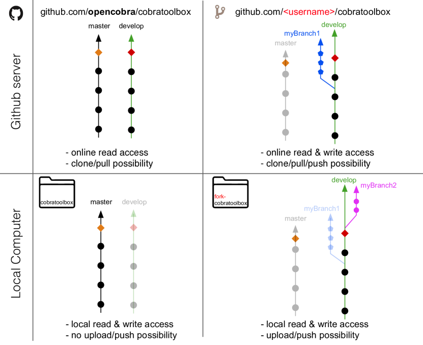
Figure 7: The openCOBRA repository and the fork of a contributor located on the Github server can be cloned to the local computer as cobratoolbox and fork-cobratoolbox folders, respectively. Each repository might contain different branches, but each repository contains the master and develop branches. Note that contributors only have read on the openCOBRA repository. The stable branch is the master branch (black branch), while the development of code is made on the develop branch (green branch). The master branch shall be checked out when using the cobratoolbox repository, whereas contributors shall create new branches originating from the develop branch (local fork-cobratoolbox directory and online <username>/cobratoolbox repository). In the present example, myBranch1 (blue branch) has already been pushed to the forked repository on the Github server, while myBranch2 (pink branch) is only present locally. The branch myBranch1 may be merged into the develop branch of the openCOBRA repository through opening a pull request. In order to submit the contributions (commits) on myBranch2, the contributor must first push the commits to the forked repository (https://github.com/<username>/cobratoolbox) before opening a pull request. Any commit made on the develop branch (red square) will be merged to the master branch if the develop branch is stable overall (orange square).

1. A user of the COBRA Toolbox

   1. The openCOBRA repository (https://github.com/opencobra/cobratoolbox) is a public repository that is read-only. Once the openCOBRA repository has been installed (as explained in Steps Initialisation of the COBRA Toolbox   TIMING $5-30$ s-Verify and test the COBRA Toolbox   TIMING $\sim 10^{3}$ s) in the folder cobratoolbox, all branches (including master and develop) are available locally. In the local folder cobratoolbox, the user has read and write access, but cannot push eventual changes back to the openCOBRA repository. It is the default and stable master branch only that should be used. The local copy located in the cobratoolbox directory can be updated (both branches).

2. A contributor or a developer of the COBRA Toolbox

   1. In order to make changes to the openCOBRA repository, or, in other words,
      tribute, you must obtain your own personal copy first. You must register on the Github website (https://github.com) in order to obtain a username. First, click on the button FORK at the top right corner of the official openCOBRA repository website (https://github.com/opencobra/cobratoolbox) in order to create a personal copy (or fork) with write and read access of the openCOBRA repository. This copy is accessible under https://github.com/<username>/cobratoolbox. These branches can be accessed by following the procedure [2] (see Step 7).

After initialisation of the MATLAB.devTools, the user and developer may have two folders: a cobratoolbox folder with the stable master branch checked out, and a fork-cobratoolbox folder with the develop branch checked out. Detailed instructions for troubleshooting and/or contributing to the COBRA Toolbox using the terminal (or shell) are provided in Supplementary Manual 3.

After the official openCOBRA version of the COBRA Toolbox has been installed, it is possible to install the MATLAB.devTools from within MATLAB:

⬇

installDevTools

With this command, the directory MATLAB.devTools is created next to the cobratoolbox installation directory. The MATLAB.devTools can also be installed from the terminal (or shell):

⬇

it clone git@github.com:opencobra/MATLAB.devTools

CRITICAL STEP A working internet connection is required and git and curl must be installed. Installation instructions are provided on the main repository page of the MATLAB.devTools. A valid passphrase-less SSH key must be set in the Github account settings in order to contribute without entering a password while securely communicating with the Github server.  ? TROUBLESHOOTING

98$\leavevmode\nobreak\ |$  The MATLAB.devTools are configured on the fly or whenever the configuration details are not present. The first time a user runs
tribute, the personal repository (fork) is downloaded (cloned) into a new folder named fork-cobratoolbox at the location specified by the user. In this local folder, both master and develop branches exist, but it is the develop branch that is automatically selected (checked out). Any new contributions are derived from the develop branch.

Initialising a contribution using the MATLAB.devTools is straightforward. In MATLAB, type:

⬇

contribute % then select procedure [1]

If the MATLAB.devTools are already configured, procedure $[1]$ updates the fork (if necessary) and initialises a new branch with a name requested during the process. Once the contribution is initialised, files can be added, modified or deleted in the folder fork-cobratoolbox. A contribution is successfully initialised when the user is presented with a brief summary of configuration details. Instructions on how to proceed are also provided.

CRITICAL STEP The location of the fork must be specified as the root directory. There will be a warning issued if the path already contains another git-tracked repository. ? TROUBLESHOOTING

99$\leavevmode\nobreak\ |$  An existing contribution can be continued after a while. This step is particularly important in order to retrieve all changes that have been made to the openCOBRA repository in the meantime.

⬇

contribute % then select procedure [2]

Procedure [2] pulls all changes from the openCOBRA repository, and rebases the existing contribution. In other words, existing commits are shifted forward and placed after all commits made on the develop branch of the openCOBRA repository.

CRITICAL STEP Before attempting to continue working on an existing feature, make sure that you published your commits as explained in Step 7. ? TROUBLESHOOTING

100$\leavevmode\nobreak\ |$  Publishing a contribution means uploading the incremental code changes to the fork. The changes are available in public, but not yet available in the openCOBRA repository. A contribution may only be accepted in the official repository once a pull request has been submitted. It is not necessary to open a pull request if you want to simply upload your contribution to your fork.

⬇

contribute % then select procedure [3]

When running procedure $[3]$, you have two options:

1. Simple contribution without opening a pull request

   1. All changes to the code are individually listed and the user is asked explicitly which changes shall be added to the commit. Once all changes have been added, a commit message must be entered. Upon confirmation, the changes are pushed to the online fork automatically.

2. Publishing and opening a pull request

   1. The procedure for submitting a pull request is the same as Option (A) with the difference that when selecting to open a pull request, a link is provided that leads to a pre-configured website according to the contributing guidelines. The pull request is then one click away.

CRITICAL STEP After following procedures $[1]$ and $[2]$, all changes should be published using procedure $[3]$ before stopping to work on that contribution. When following procedure $[3]$, the incremental changes are uploaded to the remote server. It is advised to publish often, and make small incremental changes to the code. There is no need for opening a pull request immediately (Option A) if there are more changes to be made. A pull request may be opened at any time, even manually and directly from the Github website. ? TROUBLESHOOTING

101$\leavevmode\nobreak\ |$  If a contribution has been merged into the develop branch of the openCOBRA repository (accepted pull request), the contribution (feature or branch) can be safely deleted both locally and remotely on the fork by running
tribute and selecting procedure $[4]$.

Note that deleting a contribution deletes all the changes that have been made on that feature (branch). It is not possible to selectively delete a commit using the MATLAB.devTools. Instead, create a new branch by following procedure $[1]$ (see Step 7), and follow the instructions to cherry-pick in the Supplementary Manual 3.

CRITICAL STEP Make sure that your changes are either merged or saved locally if you need them. Once procedure [4] is concluded, all changes on the deleted branch are removed, both locally and remotely. No commits can be recovered. ? TROUBLESHOOTING

102$\leavevmode\nobreak\ |$   It is sometimes useful to simply update the fork without starting a new contribution. The local fork can be updated using procedure [5] of the
tribute menu.

⬇

contribute % then select procedure [5]

CRITICAL STEP Before updating your fork, make sure that no changes are present in the local directory fork-cobratoolbox. You can do so by typing:

⬇

checkStatus

If there are changes listed, publish them by selecting procedure $[3]$ of the
tribute menu as explained in Step 7.  ? TROUBLESHOOTING

Engaging with the COBRA Toolbox forum  TIMING $1-10^{2}$ s

103$\leavevmode\nobreak\ |$   The Frequently Asked Questions (FAQ) section of the documentation (https://opencobra.github.io/cobratoolbox/docs/FAQ.html) is a good starting point to find answers to questions or issues one may face.

The public forum associated with the COBRA Toolbox, available at https://groups.google.com/forum/#!forum/cobra-toolbox, is a great way to search for solutions to previously recognised problems that are similar to problems novel to the user. This is especially so with respect to recent installation and configuration issues that have arisen due to asynchronous development of the many software packages integrated with the COBRA Toolbox.

104$\leavevmode\nobreak\ |$  Suggest new solutions to problems

1. Post your question to the online COBRA Toolbox forum

   Questions posted in the forum are welcome provided that some simple guidelines are followed:

   1. Before a question can be posted, an application for membership at https://groups.google.com/forum/#!forum/cobra-toolbox is required to eliminate spam.

   2. Make the question as detailed as possible to increase the probability of a rapid and helpful reply.

   3. Append your message with the result of running
      erateSystemConfigReport so that repository maintainers are aware of the system configuration. That is often the first question that comes to mind when considering to respond.

2. Reply to a question online COBRA Toolbox forum

   1. Community contributions are welcomed to help users overcome any issues they face and are noticed by existing COBRA community members.

Generally, responses to questions can be expected within 1-2 days of posting, provided that posting guidelines are followed.

 ? TROUBLESHOOTING

Step	Problem	Possible reason	Solution
Initialisation of the COBRA Toolbox   TIMING $5-30$ s$\leavevmode\nobreak\ |$	The tCobraToolbox function displays warnings or error messages.	Incompatible third-party software or improperly configured system.	First, read the output of the initialisation script in the command window. Any warning or error messages, though often brief, may point toward the source of the problem during initialisation if read literally. Second, verify that all software versions are supported and have been correctly installed, as described in the MATERIALS section. Third, ensure that you are using the latest version of the COBRA Toolbox, cf. Steps Contributing to the COBRA Toolbox with MATLAB.devTools   TIMING $1-30$ s-7. Fourth, verify and test the COBRA Toolbox, as described in Step Verify and test the COBRA Toolbox   TIMING $\sim 10^{3}$ s. Finally, if nothing else works, consult the COBRA Toolbox forum, as described in Steps Engaging with the COBRA Toolbox forum  TIMING $1-10^{2}$ s- Engaging with the COBRA Toolbox forum  TIMING $1-10^{2}$ s.
Verify and test the COBRA Toolbox   TIMING $\sim 10^{3}$ s$\leavevmode\nobreak\ |$	Some tests are listed as failed when running tAll.	Some third party dependencies are not properly installed or the system is improperly configured.	Verify that all required software has been correctly installed as described in the MATERIALS section. The specific test can then be run individually to determine the exact cause of the error. If the error can be fixed, try to use the MATLAB.devTools and contribute a fix. Further details on how to approach submitting a contribution are given in Steps Contributing to the COBRA Toolbox with MATLAB.devTools   TIMING $1-30$ s-7. If the error cannot be determined, reach out to the community as explained in Steps Engaging with the COBRA Toolbox forum  TIMING $1-10^{2}$ s- Engaging with the COBRA Toolbox forum  TIMING $1-10^{2}$ s.
Importing a reconstruction or a model   TIMING $10-10^{2}$ s$\leavevmode\nobreak\ |$	The dCbModelfunction fails to import a model.	The input file is not correctly formatted or the SBML file format is not supported.	Specifications for Excel sheets accepted by the COBRA Toolbox can be found on Github (opencobra.github.io/cobratoolbox/docs/COBRAModelFields.html). Files with legacy SBML formats can be imported, but some information from the SBML file might be lost. In addition to constraint-based information encoded by fields of the fbc package, the COBRA-style annotations introduced in the COBRA Toolbox 2.0[5] are supported for backward compatibility. Some information is still stored in this type of annotations. The data specified with the latest version of the fbc package is used in preference to other fields, e.g., legacy COBRA-style notes which may contain similar data.
Exporting a reconstruction or a model   TIMING $10-10^{2}$ s$\leavevmode\nobreak\ |$	The teCbModel function fails to export a model.	Some of the required fields of the el structure are missing or the model contains invalid data.	Before a reconstruction or model is exported, a summary of invalid data in the model can be obtained by running ifyModel(model). A list of required fields for the el structure is presented in Table 3.
Select a double- or quad-precision optimisation solver  TIMING $1-5$ s$\leavevmode\nobreak\ |$	The Minos or dMinos interfaces are not working as intended.	The binaries might not be compatible with your operating system.	Make sure that all relevant system requirements described in the MATERIALS section are satisfied. If you are still unable to use the respective interfaces, reach out to the community as explained in Steps Engaging with the COBRA Toolbox forum  TIMING $1-10^{2}$ s- Engaging with the COBRA Toolbox forum  TIMING $1-10^{2}$ s.
Identify stoichiometrically consistent and inconsistent reactions  TIMING $1-10^{5}s$$\leavevmode\nobreak\ |$   A)	The dSExRxnInd function fails to identify some exchange, demand and sink reactions.	Some exchange, demand and sink reactions do not start with any of anticipated prefixes.	Try an alternative approach.
Identify stoichiometrically consistent and inconsistent reactions  TIMING $1-10^{5}s$$\leavevmode\nobreak\ |$   B)	The function ckMassChargeBalance returns wrong results.	Some formulae are missing or a formula is incorrectly specified, leading to one or more reactions to be incorrectly identified as being elementally balanced.	Try an alternative approach.
Identify stoichiometrically consistent and inconsistent reactions  TIMING $1-10^{5}s$$\leavevmode\nobreak\ |$   C)	Erroneous predictions.	Inadvertent violation of the steady-state mass conservation constraint.	Manually inspect the reaction formulae for each reaction to identify any obviously mass imbalanced reactions, omit them from the reconstruction and run dStoichConsistentSubset again.
Flux balance analysis  TIMING $1-10^{2}$ s$\leavevmode\nobreak\ |$	The solution status given by solution.stat is $-1$.	A too short runtime limit has been set or numerical issues happened during the optimisation procedure.	Check the value of solution.origStat and compare it with the documentation provided by the solver in use for further information. If one is solving with a double precision solver a model that could be multi-scale but is not yet recognised as such, then solution.stat == -1 can be symptomatic of this situation. In that case, refer to Steps Check the scaling of a reconstruction   TIMING $1-10^{2}$ s-Select a double- or quad-precision optimisation solver  TIMING $1-5$ s to learn how to numerically characterise a reconstruction model.
Uniform sampling of steady-state fluxes   TIMING $1-10^{3}$ s$\leavevmode\nobreak\ |$	The sampling distribution is not uniform (revealed by a non-uniform marginal flux distribution).	The sampling parameters ions.nSkip and ions.nSamples are set too low.	Increase the values of the ions.nSkip and ions.nSamples parameters until smooth and unimodal marginal flux distributions are obtained.
6$\leavevmode\nobreak\ |$	No reaction is found in the MUST sets.	The wild-type or mutant strain may not be enough constrained.	A solution is to add more constraints to the strains until differences in the reaction ranges are shown. If no differences are found, another algorithm might be better suited. If there is an error when running the dMust* functions, a possible reason is that the inputs are not well defined or a solver may not be set. Verify the inputs, use ngeCobraSolver to change to a commercial-grade optimisation solver (see Table 4 for a list of supported solvers).
Atomically resolve a metabolic reconstruction  TIMING $10-10^{5}$ s$\leavevmode\nobreak\ |$	Some reactions could not be mapped.	Too short runtime limit or a reaction that the algorithm could not atom map.	Increase the runtime limit of the algorithm.
Human metabolic network visualisation with ReconMap  TIMING $1-10^{2}$ s$\leavevmode\nobreak\ |$	The remote MINERVA server refuses to build a new overlay.	The text string in the ntifier input variable is not uniquely defined in your account.	Change the ntifier text string of your overlay.
7$\leavevmode\nobreak\ |$	An error occurs when run running tribute claiming that the fork cannot be reached or that the local fork cannot be found.	The local forked folder cannot be found, has been moved, or the remote fork cannot be reached.	It may occur that the configuration of the MATLAB.devTools is faulty or has been mistyped. In that case, try to reset the configuration by typing: ⬇ resetDevTools
Contributing to the COBRA Toolbox with MATLAB.devTools   TIMING $1-30$ s$\leavevmode\nobreak\ |$	An error might be thrown claiming mission denied.	The SSH key of the computer is not configured properly.	The installation of the MATLAB.devTools is dependent on a correctly configured Github account. The SSH key of the computer must be set in the Github account settings or otherwise errors will be thrown. If the git clone command works, the SSH key is properly set. In that case, delete the SSH key locally (generally located in the folder .ssh in the home directory) and remotely on Github, and generate a new SSH key.
7$\leavevmode\nobreak\ |$	Procedure $[1]$ when running tribute might not be successful.	The local fork-cobratoolbox folder is too old or has not been updated for a while.	In that case and if no local changes are present, backup and remove the local fork-cobratoolbox folder and run the tribute command again. Alternatively, try to delete the forked repository online and re-fork the openCOBRA repository. When one is sure that everything is fine, the backup can be safely deleted, but it is wise to store it for some time, in case later one realises that some updates to code have gone missing.
7$\leavevmode\nobreak\ |$	Procedure $[1]$ when running tribute might not be successful.	There are changes in the local fork-cobratoolbox folder.	Contribute the changes manually as described in the Supplementary Manual 3.
7$\leavevmode\nobreak\ |$	Procedure $[1]$ when running tribute might not be successful.	The forked repository cannot be reached online or the SSH key is not configured properly.	Set the SSH key in your Github account and make sure that the forked repository can be reached. This can easily be checked by re-cloning the MATLAB.devTools in the terminal as explained in Step Contributing to the COBRA Toolbox with MATLAB.devTools   TIMING $1-30$ s and by browsing to the forked repository online.
7$\leavevmode\nobreak\ |$	Procedure $[2]$ when running tribute might fail.	Your contribution has been deleted online, or is no longer available locally.	When the rebase process fails, the user is asked to reset the contribution, which will reset the contribution to the online version of the branch in the fork. In general, when the rebase fails there have been changes made on the openCOBRA repository that are in conflict with the local changes. You can check the status of the local repository by typing: ⬇ checkStatus If there are conflicts that you do not know how to resolve, check the official repository or ping the developers in https://groups.google.com/forum/#!forum/cobra-toolbox as explained in Steps Engaging with the COBRA Toolbox forum  TIMING $1-10^{2}$ s- Engaging with the COBRA Toolbox forum  TIMING $1-10^{2}$ s. If you already have published changes, try to submit a pull request as explained in Step 7 for developers to understand the situation. Alternatively, you can try to resolve the conflicts manually. More information on how to solve conflicts is given as Supplementary Manual 3.
7$\leavevmode\nobreak\ |$	Procedure $[3]$ when running tribute might not be successful.	The forked repository cannot be reached online or if the SSH key is not configured properly.	Check to set the SSH key in your Github account and make sure that the forked repository can be reached.
7$\leavevmode\nobreak\ |$	When opening a pull request, Github cannot automatically merge.	There have been changes made on the openCOBRA repository and on your local fork.	Submit however the pull request; another developer will help you rebase your contribution manually.
7$\leavevmode\nobreak\ |$	Procedure $[4]$ when running tribute might not be successful.	Your local changes are not yet published (committed).	Follow procedure $[3]$ of the tribute menu in order to publish your changes first as explained in Step 7.
7$\leavevmode\nobreak\ |$	Procedure $[5]$ when running tribute might not be successful.	There are some local changes that have not yet been published (committed).	Backup eventual modifications, remove the fork-cobratoolbox folder, and run the tribute command again.
7$\leavevmode\nobreak\ |$	Procedure $[5]$ when running tribute might not be successful.	Too many changes have been made in the openCOBRA repository.	Backup your modified files to a separate location, and reset your branch manually by typing in the terminal (be careful - this will delete all your changes locally, but not remotely): ⬇ it reset --hard origin/<yourBranch> Then, copy your file back into the fork-cobratoolbox folder and tribute normally.

  TIMING

Steps Initialisation of the COBRA Toolbox   TIMING $5-30$ s-Initialisation of the COBRA Toolbox   TIMING $5-30$ s, Initialisation of the COBRA Toolbox   TIMING $5-30$ s: $5-30$ s

Step Verify and test the COBRA Toolbox   TIMING $\sim 10^{3}$ s, Verify and test the COBRA Toolbox   TIMING $\sim 10^{3}$ s: $\sim 10^{3}$ s

Step Importing a reconstruction or a model   TIMING $10-10^{2}$ s, Importing a reconstruction or a model   TIMING $10-10^{2}$ s: $10-10^{2}$ s

Step Exporting a reconstruction or a model   TIMING $10-10^{2}$ s, Exporting a reconstruction or a model   TIMING $10-10^{2}$ s: $10-10^{2}$ s

Step Use of rBioNet to add reactions to a reconstruction  TIMING $1-10^{3}$ s, Use of rBioNet to add reactions to a reconstruction  TIMING $1-10^{3}$ s: $1-10^{3}$ s

Steps Use of a spreadsheet to add reactions to a reconstruction  TIMING $1-10^{3}$ s-Use of a spreadsheet to add reactions to a reconstruction  TIMING $1-10^{3}$ s, Use of a spreadsheet to add reactions to a reconstruction  TIMING $1-10^{3}$ s: $1-10^{3}$s

Steps Use of scripts with reconstruction functions  TIMING $1-10^{2}$ s-Use of scripts with reconstruction functions  TIMING $1-10^{2}$ s, Use of scripts with reconstruction functions  TIMING $1-10^{2}$ s: $1-10^{2}$s

Step Check the scaling of a reconstruction   TIMING $1-10^{2}$ s, Check the scaling of a reconstruction   TIMING $1-10^{2}$ s: $1-10^{2}$ s

Step Select a double- or quad-precision optimisation solver  TIMING $1-5$ s, Select a double- or quad-precision optimisation solver  TIMING $1-5$ s: $1-5$ s

Step Identify stoichiometrically consistent and inconsistent reactions  TIMING $1-10^{5}s$, Identify stoichiometrically consistent and inconsistent reactions  TIMING $1-10^{5}s$: $1-10^{5}$ s

Step Identify stoichiometrically consistent and inconsistent molecular species  TIMING $1-10^{3}\leavevmode\nobreak\$s, Identify stoichiometrically consistent and inconsistent molecular species  TIMING $1-10^{3}\leavevmode\nobreak\$s: $1-10^{3}$ s

Step Set simulation constraints  TIMING $1-10^{3}$ s, Set simulation constraints  TIMING $1-10^{3}$ s: $1-10^{3}$ s

Step Identify molecular species that leak, or siphon, across the boundary of the model  TIMING $1-10^{3}$ s, Identify molecular species that leak, or siphon, across the boundary of the model  TIMING $1-10^{3}$ s: $1-10^{3}$ s

Step Identify flux inconsistent reactions  TIMING $1-10^{3}$ s, Identify flux inconsistent reactions  TIMING $1-10^{3}$ s: $1-10^{3}$ s

Steps Flux balance analysis  TIMING $1-10^{2}$ s-Flux balance analysis  TIMING $1-10^{2}$ s, Flux balance analysis  TIMING $1-10^{2}$ s: $1-10^{2}$ s

Step Relaxed flux balance analysis  TIMING $1-10^{3}$ s, Relaxed flux balance analysis  TIMING $1-10^{3}$ s: $1-10^{3}$ s

Step Sparse flux balance analysis  TIMING $1-10^{3}$ s, Sparse flux balance analysis  TIMING $1-10^{3}$ s: $1-10^{3}$ s

Steps Identify dead-end metabolites and blocked reactions  TIMING $\sim$$10^{2}$ s-Identify dead-end metabolites and blocked reactions  TIMING $\sim$$10^{2}$ s, Identify dead-end metabolites and blocked reactions  TIMING $\sim$$10^{2}$ s: $\sim$$10^{2}$ s

Steps Gap fill a metabolic network  TIMING $10^{2}-10^{5}$ s-Gap fill a metabolic network  TIMING $10^{2}-10^{5}$ s, Gap fill a metabolic network  TIMING $10^{2}-10^{5}$ s: $10^{2}-10^{5}$ s

Steps Extracellular metabolomic data  TIMING $10^{3}-10^{5}$ s-Extracellular metabolomic data  TIMING $10^{3}-10^{5}$ s, Extracellular metabolomic data  TIMING $10^{3}-10^{5}$ s: $10^{3}-10^{5}$ s

Steps 3-4, Conceptual overview of the main steps involved in the unsteady-state flux balance analysis (uFBA) method. : $10^{2}-10^{4}$ s

Step Integration of transcriptomic and proteomic data  TIMING $10^{2}-10^{4}$ s, Integration of transcriptomic and proteomic data  TIMING $10^{2}-10^{4}$ s: $10^{2}-10^{4}$ s

Steps Adding biological constraints to a flux balance model   TIMING $\sim 10^{2}$ s-Adding biological constraints to a flux balance model   TIMING $\sim 10^{2}$ s, Adding biological constraints to a flux balance model   TIMING $\sim 10^{2}$ s: $\sim 10^{2}$ s

Steps Qualitative chemical and biochemical fidelity testing  TIMING $10^{2}-10^{3}$ s-Qualitative chemical and biochemical fidelity testing  TIMING $10^{2}-10^{3}$ s, Qualitative chemical and biochemical fidelity testing  TIMING $10^{2}-10^{3}$ s: $10^{2}-10^{3}$ s

Steps Quantitative biochemical fidelity testing  TIMING $10^{2}-10^{3}$ s-Quantitative biochemical fidelity testing  TIMING $10^{2}-10^{3}$ s, Quantitative biochemical fidelity testing  TIMING $10^{2}-10^{3}$ s: $10^{2}-10^{3}$ s

Step MinSpan Pathways: a sparse basis of the nullspace of a stoichiometric matrix  TIMING $10^{2}-10^{4}$ s, MinSpan Pathways: a sparse basis of the nullspace of a stoichiometric matrix  TIMING $10^{2}-10^{4}$ s: $10^{2}-10^{4}$ s

Step Low dimensional flux variability analysis  TIMING $1-10^{3}$ s, Low dimensional flux variability analysis  TIMING $1-10^{3}$ s: $1-10^{3}$ s

Step High dimensional flux variability analysis  TIMING $1-10^{5}$ s, High dimensional flux variability analysis  TIMING $1-10^{5}$ s: $1-10^{5}$ s

Step Uniform sampling of steady-state fluxes   TIMING $1-10^{3}$ s, Uniform sampling of steady-state fluxes   TIMING $1-10^{3}$ s: $1-10^{3}$ s

Steps 6-6, In the OptForce procedure, the MUST sets are determined by contrasting the flux ranges obtained using flux variability analysis (FVA) of a wild-type (blue bars) and an overproducing strain (red bars). The first order MUST sets (top panel) are denoted MUST${}^{\textrm{L}}$ and MUST${}^{\textrm{U}}$. For instance, a reaction belongs to the MUST${}^{\textrm{U}}$ set if the upper bound of the flux range in the wild-type is less than the lower bound of the flux range of the overproducing strain. The center and bottom panels show all possible second order MUST sets.: $10-10^{5}$ s

Steps Atomically resolve a metabolic reconstruction  TIMING $10-10^{5}$ s-Atomically resolve a metabolic reconstruction  TIMING $10-10^{5}$ s, Atomically resolve a metabolic reconstruction  TIMING $10-10^{5}$ s: $10-10^{5}$ s

Steps Thermodynamically constrain a metabolic model  TIMING $1-10^{3}$ s-Thermodynamically constrain a metabolic model  TIMING $1-10^{3}$ s, Thermodynamically constrain a metabolic model  TIMING $1-10^{3}$ s: $1-10^{3}$ s

Step Convert a flux balance model into a kinetic model   TIMING $1-10^{3}$ s, Convert a flux balance model into a kinetic model   TIMING $1-10^{3}$ s: $1-10^{3}$ s

Step Compute a non-equilibrium kinetic steady state   TIMING $1-10^{3}$ s, Compute a non-equilibrium kinetic steady state   TIMING $1-10^{3}$ s: $1-10^{3}$ s

Step Compute a moiety conserved non-equilibrium kinetic steady state   TIMING $1-10^{3}$ s, Compute a moiety conserved non-equilibrium kinetic steady state   TIMING $1-10^{3}$ s: $1-10^{3}$ s

Steps Human metabolic network visualisation with ReconMap  TIMING $1-10^{2}$ s-Human metabolic network visualisation with ReconMap  TIMING $1-10^{2}$ s, Human metabolic network visualisation with ReconMap  TIMING $1-10^{2}$ s: $1-10^{2}$ s

Steps Variable scope visualisation of a network with Paint4Net  TIMING $1-10^{3}$ s-Variable scope visualisation of a network with Paint4Net  TIMING $1-10^{3}$ s, Variable scope visualisation of a network with Paint4Net  TIMING $1-10^{3}$ s: $1-10^{3}$ s

Steps Contributing to the COBRA Toolbox with MATLAB.devTools   TIMING $1-30$ s-7, Contributing to the COBRA Toolbox with MATLAB.devTools   TIMING $1-30$ s: $1-30$ s

ANTICIPATED RESULTS

Initialisation of the COBRA Toolbox   TIMING $5-30$ s

Initialisation of the COBRA Toolbox   TIMING $5-30$ s$\leavevmode\nobreak\ |$  The initialisation step automatically checks the configuration of all of the required and some of the optional software dependencies. During initialisation, all git submodules are updated. The solver paths are set when available and compatible. A system-dependent table with the solver status is returned, together with solver suggestions as shown in Figure 8. The user is also presented with options to update the COBRA Toolbox.

Figure 8: Output of initialisation of the COBRA Toolbox with
tCobraToolbox.

Initialisation of the COBRA Toolbox   TIMING $5-30$ s$\leavevmode\nobreak\ |$  A list of solvers assigned to solve each class of optimisation solvers is returned:

⬇

ined solvers are:

CBT_LP_SOLVER: gurobi

CBT_MILP_SOLVER: gurobi

CBT_QP_SOLVER: qpng

CBT_MIQP_SOLVER: gurobi

CBT_NLP_SOLVER: matlab

Verify and test the COBRA Toolbox   TIMING $\sim 10^{3}$ s$\leavevmode\nobreak\ |$  The test suite starts by initialising the COBRA Toolbox and thereafter, all of the tests are run. At the end of the test run, a comprehensive summary table is presented in which the respective tests and their test outcome is shown. On a fully configured system that is compatible with the most recent version of the COBRA Toolbox, all tests should pass. It may not be necessary to have a fully configured system to use one’s particular subset of methods.

Importing a reconstruction or a model   TIMING $10-10^{2}$ s

Importing a reconstruction or a model   TIMING $10-10^{2}$ s$\leavevmode\nobreak\ |$   The reconstruction or model is loaded into the MATLAB workspace within a structure named
el, irrespective of whether the
eName specified a reconstruction or model. The model structure should contain all of the information in different fields. Table 3 provides an overview of the individual model fields and their content. Very large SBML models may take some time to load.

Exporting a reconstruction or a model   TIMING $10-10^{2}$ s$\leavevmode\nobreak\ |$   An exported file containing the information from the model in the location and format specified by the
eName.

Check the scaling of a reconstruction   TIMING $1-10^{2}$ s

Check the scaling of a reconstruction   TIMING $1-10^{2}$ s$\leavevmode\nobreak\ |$   The
ckScaling function returns a
cisionEstimate string that is either
'double' or
'quad'. The scaling estimate is based on the order of magnitude of the ratio of the maximum and minimum row and column scaling coefficients, which are determined such that the scaled stoichiometric matrix has entries close to unity. In addition, a summary of scaling properties included in
lingProperties may be returned.

Select a double- or quad-precision optimisation solver  TIMING $1-5$ s

Select a double- or quad-precision optimisation solver  TIMING $1-5$ s$\leavevmode\nobreak\ |$   If the selected solver is installed,
verStatus == 1 will be returned, the solver interface to MATLAB is configured correctly, and the solver is compatible with the system environment. If the
Minos solver has been selected and
verStatus == 1, then LP problem solutions are computed somewhat slower than with a double precision solver, but with the advantage that solutions are computed with a feasibility and optimality tolerance of $10^{-15}$, which becomes an advantage for a multi-scale model, where the typical tolerance of $10^{-6}$ for a double precision solver may be insufficient.

Identify stoichiometrically consistent and inconsistent molecular species  TIMING $1-10^{3}\leavevmode\nobreak\$s

Identify stoichiometrically consistent and inconsistent molecular species  TIMING $1-10^{3}\leavevmode\nobreak\$s$\leavevmode\nobreak\ |$   Any molecular species corresponding to a non-zero entry within
nsistentMetBool is always involved in mass imbalanced reactions indicating that the stoichiometry is misspecified. Double check the chemical formulae involved in the corresponding reactions to ensure that, e.g., the stoichiometry for protons, cofactors, etc., leads to balanced reactions.

Identify flux inconsistent reactions  TIMING $1-10^{3}$ s$\leavevmode\nobreak\ |$  Any non-zero entry in
xInConsistentRxnBool indicates a flux inconsistent reaction, i.e., a reaction that does not admit a non-zero flux. Blocked reactions can be resolved by manual reconstruction[42], algorithmic reconstruction[45], or a combination of both.

Sparse flux balance analysis  TIMING $1-10^{3}$ s

Sparse flux balance analysis  TIMING $1-10^{3}$ s$\leavevmode\nobreak\ |$   There should be no such cycle in a network with bounds that are sufficiently constrained. Figure  9 illustrates the cycle obtained from Recon3D with all internal reaction bounds set to zero.

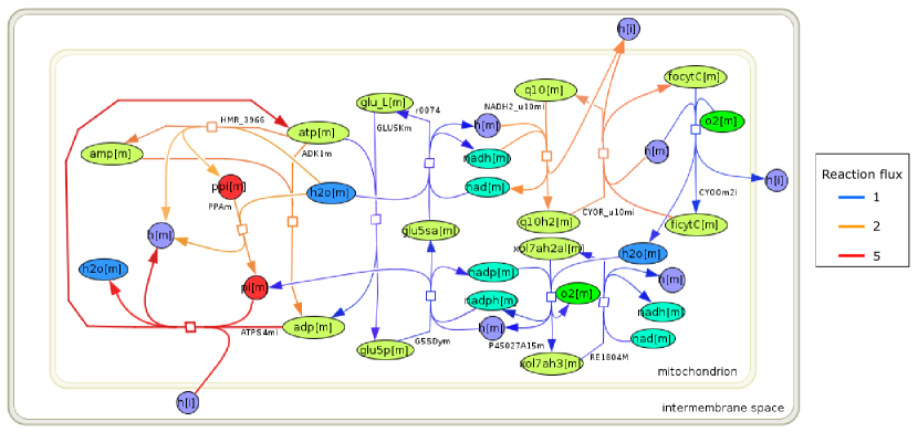
Figure 9: An energy generating stoichiometrically balanced cycle. The smallest stoichiometrically balanced cycle that produces ATP at a maximal rate using the ATP synthase reaction, in Recon3D, with all internal reactions. All metabolite and reaction abbreviations are primary keys in the Virtual Metabolic Human database (https://vmh.uni.lu): reaction abbreviation, reaction name: ADK1m, adenylate kinase, mitochondrial; G5SDym, glutamate-5-semialdehyde dehydrogenase, mitochondrial; GLU5Km, glutamate 5-kinase, mitochondrial; P45027A15m, 5-beta-cytochrome P450, family 27, subfamily A, polypeptide 1; PPAm, inorganic diphosphatase; r0074, L-glutamate 5-semialdehyde:NAD+ oxidoreductase; HMR_3966, nucleoside-triphosphate giphosphatase; ATPS4mi, ATP synthase (four protons for one ATP); CYOR_u10mi, ubiquinol-6 cytochrome c reductase, Complex III; NADH2_u10mi, NADH dehydrogenase, mitochondrial; CYOOm2i, cytochrome c oxidase, mitochondrial complex IV.

Integration of transcriptomic and proteomic data  TIMING $10^{2}-10^{4}$ s

Integration of transcriptomic and proteomic data  TIMING $10^{2}-10^{4}$ s$\leavevmode\nobreak\ |$  
ateTissueSpecificModel returns a COBRA model which is constrained with the context of the data provided to it. Usually, this means enrichment of reactions with high expression and omission of reactions with low expression profiles. Each method returns a flux consistent model, hence it is likely that certain reactions, without experimental evidence, are added to the context-specific model in order to enable non-zero net flux through reactions for which supporting experimental evidence for activity exists.

Quantitative biochemical fidelity testing  TIMING $10^{2}-10^{3}$ s

Quantitative biochemical fidelity testing  TIMING $10^{2}-10^{3}$ s$\leavevmode\nobreak\ |$   For the
on3Dmodel, the anticipated yield is $32$ ATP per unit of glucose, which compares favourably to the ATP yield of $31$ ATP obtained from the biochemical literature.

Uniform sampling of steady-state fluxes   TIMING $1-10^{3}$ s

Uniform sampling of steady-state fluxes   TIMING $1-10^{3}$ s$\leavevmode\nobreak\ |$   The marginal flux distributions for each reaction should be smooth and uni-modal for any biochemical network with feasible set $\Omega\coloneqq\left\{v\mid Sv=0;\leavevmode\nobreak\ l\leq v\leq u\right\}$.

In the OptForce procedure, the MUST sets are determined by contrasting the flux ranges obtained using flux variability analysis (FVA) of a wild-type (blue bars) and an overproducing strain (red bars). The first order MUST sets (top panel) are denoted MUST${}^{\textrm{L}}$ and MUST${}^{\textrm{U}}$. For instance, a reaction belongs to the MUST${}^{\textrm{U}}$ set if the upper bound of the flux range in the wild-type is less than the lower bound of the flux range of the overproducing strain. The center and bottom panels show all possible second order MUST sets.

6$\leavevmode\nobreak\ |$   The identified reaction is
t, i.e., a transporter for succinate (an intuitive solution). However, changing the parameters will enable
Force to find non-intuitive solutions.

In the OptForce procedure, the MUST sets are determined by contrasting the flux ranges obtained using flux variability analysis (FVA) of a wild-type (blue bars) and an overproducing strain (red bars). The first order MUST sets (top panel) are denoted MUST${}^{\textrm{L}}$ and MUST${}^{\textrm{U}}$. For instance, a reaction belongs to the MUST${}^{\textrm{U}}$ set if the upper bound of the flux range in the wild-type is less than the lower bound of the flux range of the overproducing strain. The center and bottom panels show all possible second order MUST sets.

6$\leavevmode\nobreak\ |$   Figure 10 illustrates the interventions predicted by the OptForce method for succinate overproduction in the AntCore E. coli model under aerobic conditions.

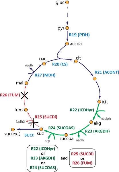
Figure 10: The interventions predicted by the OptForce method for succinate overproduction in E. coli (AntCore model) under aerobic conditions. Reactions that need to be up-regulated (green arrows and labels) and knocked out (red arrows and labels) are shown in this simplified metabolic map. The strategies include up-regulation of reactions generating succinate such as isocitrate dehydrogenase (R2), $\alpha$-ketoglutarate dehydrogenase or succinyl-CoA synthetase, along with knockout of reactions draining succinate such as succinate dehydrogenase or fumarate hydratase. Note that each of these reactions may associate with one or more genes in E. coli.

Thermodynamically constrain a metabolic model  TIMING $1-10^{3}$ s

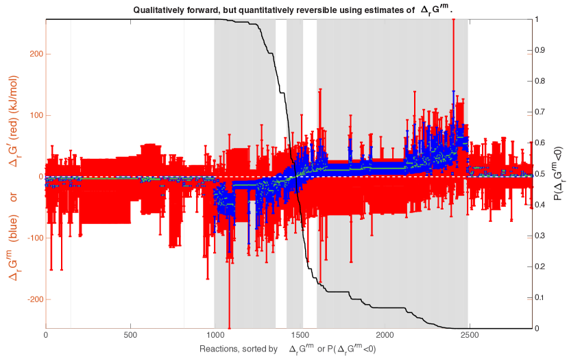
Figure 11: Qualitatively forward, quantitatively reverse reactions in a multi-compartmental, genome-scale model. In Recon3D, the transformed reaction Gibbs energy could be estimated for $7,215$ reactions. Of these reactions, $2,868$ reactions were qualitatively assigned to be forward in the reconstruction, but were quantitatively assigned to be reversible using subcellular compartment specific thermodynamic parameters, the component contribution method, and broad bounds on metabolite concentrations ($10^{-5}-0.02$ mol/L), except for certain cofactors. The geometric mean (green) and feasible range (between maximum and minimum) of estimated millimolar standard transformed reaction Gibbs energy ($\Delta_{r}G^{\prime m}$, blue) and transformed reaction Gibbs energy ($\Delta_{r}G^{\prime}$, red) are illustrated. The relative uncertainty in metabolite concentrations versus uncertainty in thermochemical estimates is reflected by the relative breadth of the red and blue bars for each reaction, respectively. The reactions are rank ordered by the cumulative probability that millimolar standard transformed reaction Gibbs energy is less than zero, $P(\Delta_{r}G^{\prime m}<0)$, (black descending line from left to right). This assumes that all metabolites are at a millimolar concentration ($1mM$) and a Gaussian error is assumed in component contribution estimates. In this ordering, forward transport reactions have $P(\Delta_{r}G^{\prime m}<0)=1$ (far left) and reverse transport reactions have $P(\Delta_{r}G^{\prime m}<0)=0$ (far right). In between, from left to right are biochemical reactions with decreasing cumulative probability of being forward in direction, subject to the stated assumptions. Alternative rankings are possible. The key point is to observe that the COBRA Toolbox is primed for quantitative integration of metabolomic data as the uncertainty in transformed reaction Gibbs energy associated with thermochemical estimates using the component contribution method is now significantly lower than the uncertainty associated with the assumption of broad concentration range.

Thermodynamically constrain a metabolic model  TIMING $1-10^{3}$ s$\leavevmode\nobreak\ |$   Thermodynamically constrained flux predictions can differ markedly from those obtained with flux balance analysis. An open challenge is acquisition of sufficient thermochemical training data as well as sufficient quantitative metabolomic data, such that estimates of transformed reaction Gibbs energies can be made with sufficiently low uncertainty to constrain reaction directionality with high confidence. The degree of confidence typically differs markedly between reactions. Therefore, a pragmatic approach to rank order reaction directionality assignments by the probability that the thermodynamically assigned reaction directionality is forward, reversible or reverse (see Figure 11 for an application to Recon3D).

Human metabolic network visualisation with ReconMap  TIMING $1-10^{2}$ s

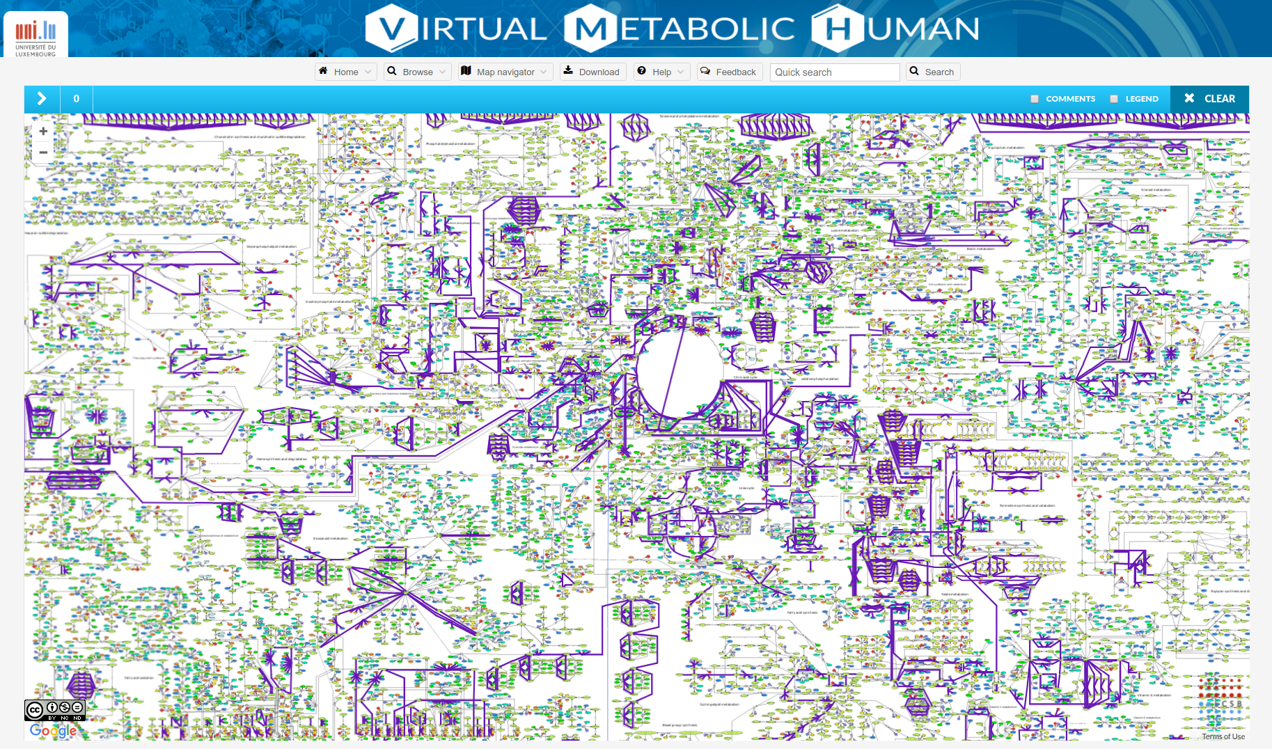
Figure 12: Overlay of the flux vector for maximum ATP synthase flux, using flux balance analysis with regularisation of the flux vector. Active fluxes are highlighted (purple).

Human metabolic network visualisation with ReconMap  TIMING $1-10^{2}$ s$\leavevmode\nobreak\ |$   Figure 12 illustrates the overlay of an optimal regularised flux balance analysis solution overlain within ReconMap within a web browser window.

Variable scope visualisation of a network with Paint4Net  TIMING $1-10^{3}$ s

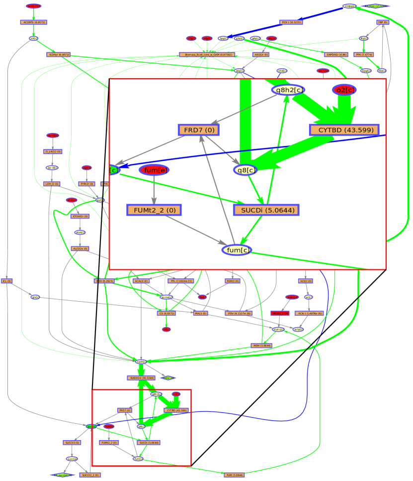
Figure 13: Selective scope visualisation of the E. coli core model model by Paint4Net. Rectangles represent reactions with rates of fluxes in brackets; the red rectangles represent reactions with only one metabolite; ellipses represent metabolites; the red ellipses represent dead end metabolites; grey edges represent zero-rate fluxes; green edges represent positive-rate (forward) fluxes; and blue edges represent negative-rate (backward) fluxes. Network visualisation also enables zoom to specific regions.

Variable scope visualisation of a network with Paint4Net  TIMING $1-10^{3}$ s$\leavevmode\nobreak\ |$   Figure 13 illustrates a fragment of a Paint4Net visualisation contextualised using a flux vector to control the thickness and colour of edges representing reactions. In the visualisation, one can discover the isolated parts of network without any flux, as well as cycles running without any substrate.

ACKNOWLEDGEMENTS

The Reproducible Research Results (R3) team, in particular Christophe Trefois and Yohan Jarosz, of the Luxembourg Centre for Systems Biomedicine, is acknowledged for their help in setting up the virtual machine and the Jenkins server. This study was funded by the National Centre of Excellence in Research (NCER) on Parkinson’s disease, the U.S. Department of Energy, Offices of Advanced Scientific Computing Research and the Biological and Environmental Research as part of the Scientific Discovery Through Advanced Computing program, grant no. DE-SC0010429. This project has also received funding from the European Union’s HORIZON 2020 research and innovation programme under grant agreement No 668738, the Fonds National de la Recherche grant O16/11402054, and the Luxembourg National Research Fund (FNR) ATTRACT program (FNR/A12/01) and OPEN (FNR/O16/11402054) grants. Nathan E. Lewis has been supported by NIGMS (R35 GM119850) and the Novo Nordisk Foundation (NNF10CC1016517). Anne Richelle has been supported by the Lilly Innovation Fellows Award. Francisco Planes has been supported by the Minister of Economy and Competitiveness of Spain (BIO2016-77998-R) and ELKARTEK Programme of the Basque Government (KK-2016/00026). Iõigo Apaolaza has been supported by the Basque Government predoctoral grant (PRE_2016_2_0044). Bernhard Ø. Palsson has been supported by the Novo Nordisk Foundation through the Center for Biosustainability at the Technical University of Denmark (NNF10CC1016517).

These authors contributed equally to this work: Laurent Heirendt & Sylvain Arreckx

AUTHOR CONTRIBUTIONS

Author	Contributions
Sylvain Arreckx	Continuous integration, code review, opencobra.github.io/cobratoolbox, Jenkins, Documenter.py, changeCobraSolver, pull request support, tutorials, tests, coordination, manuscript, initCobraToolbox.
Laurent Heirendt	Continuous integration, code review, fastFVA (new version, test & integration), MATLAB.devTools, opencobra.github.io, tutorials, tests, pull request support, coordination, manuscript, initCobraToolbox, forum support.
Thomas Pfau	IO and transcriptomic integration, tutorials, tutorial reviews, IO and transcriptomic integration sections of manuscript, forum support, pull request support, code review.
Sebastián N. Mendoza	Development and update of strain design algorithms, GAMS and MATLAB integration, tutorials.
Anne Richelle	Transcriptomic data integration methods, tutorials, transcriptomic integration section of manuscript, RuMBA, pFBA, metabolic tasks, tutorial review.
Almut Heinken	Multispecies modelling code contribution, tutorial review, testing.
Hulda S. Haraldsdóttir	Thermodynamics, conserved moiety and sampling methods.
Jacek Wachowiak	Documentation.
Sarah M. Keating	SBML input-output support.
Vanja Vlasov	Tutorials.
Stefania Magnusdóttir	Multispecies modelling, tutorial review, testing.
Chiam Yu Ng	Strain design code review, tutorial review, manuscript (OptForce/biotech introduction).
German Preciat	Tutorials and chemoinformatics for metabolite structures and atom mapping data.
Alise Žagare	Metabolic cartography.
Siu H.J. Chan	Solution navigation, multispecies modelling code, tutorial review.
Maike K. Aurich	Metabolomic data integration.
Catherine M. Clancy	Tutorials, testing.
Jennifer Modamio	Metabolic cartography and human metabolic network visualisation tutorials.
John T. Sauls	modelBorgifier code and tutorial.
Alberto Noronha	Virtual metabolic human interoperability.
Aarash Bordbar	MinSpan method and tutorial, supervision on uFBA method and tutorial.
Benjamin Cousins	CHRR uniform sampling.
Diana C. El Assal	Tutorials.
Luis V. Valcarcel	Tutorials and genetic MCSs implementation.
Iñigo Apaolaza	Tutorials and genetic MCSs implementation.
Susan Ghaderi	Interoperability with CellNetAnalyzer.
Masoud Ahookhosh	Adaptive Levenberg-Marquardt solver.
Marouen Ben Guebila	Tutorial reviews.
Andrejs Kostromins	Paint4Net code and tutorial.
Nicolas Sompairac	Development of metabolomic cartography tool and tutorial.
Hoai M. Le	Cardinality optimisation solver.
Ding Ma	Quad precision solvers.
Yuekai Sun	Multiscale flux balance analysis reformulation.
Lin Wang	Strain design code review, tutorial review, manuscript (OptForce).
James T. Yurkovich	uFBA method and tutorial.
Miguel A.P. Oliveira	Tutorial.
Phan T. Vuong	Adaptive Levenberg-Marquardt solvers, boosted difference of convex optimisation solver.
Lemmer P. El Assal	Chemoinformatic data integration, documentation.
Inna Kuperstein	Development of metabolomic cartography tool and tutorial.
Andrei Zinovyev	Development of metabolomic cartography tool and tutorial.
H. Scott Hinton	Tutorials.
William A. Bryant	Code refinement.
Francisco J. Aragón Artacho	Duplomonotone equation solver, boosted difference of convex optimisation solver, adaptive Levenberg-Marquardt solvers.
Francisco J. Planes	Academic Supervision, tutorials and genetic MCSs implementation.
Egils Stalidzans	Academic supervision, Paint4Net, tutorial.
Alejandro Maass	Academic supervision.
Santosh Vempala	Academic supervision, CHRR uniform sampling algorithm.
Michael Hucka	Academic supervision, SBML input-output support.
Michael A. Saunders	Academic supervision, quad precision solvers, nullspace computation, convex optimisation.
Costas D. Maranas	Academic supervision, strain design algorithms.
Nathan E. Lewis	Academic supervision and coding, transcriptomic data integration. RuMBA, pFBA, metabolic tasks, tutorial review.
Thomas Sauter	Academic supervision, FASTCORE algorithm.
Bernhard Ø. Palsson	Academic supervision, openCOBRA stewardship.
Ines Thiele	Academic supervision, tutorials, code contribution, manuscript.
Ronan M.T. Fleming	Conceptualisation, lead developer, academic supervision, software architecture, code review, sparse optimisation, nullspace computation, thermodynamics, variational kinetics, fastGapFill, sampling, conserved moieties, network visualisation, forum support, tutorials, manuscript.

COMPETING FINANCIAL INTERESTS

The authors declare that they have no competing financial interests.

Supplementary information

Supplementary Manual 1 - MATLAB basics

Brief tutorial and guidelines on how to use the MATLAB software.

Supplementary Manual 2 - Shell or Terminal basics

Brief tutorial and guidelines on how to use the Terminal or shell.

Supplementary Manual 3 - Contributing to the COBRA Toolbox using git

Guidelines on how to use git and contribute to the COBRA Toolbox.

Supplementary Manual 1 - MATLAB basics

The following introductory material and online tutorials available at https://mathworks.com/help/matlab/getting-started-with-matlab.html are recommended to learn some of the most useful features of MATLAB. In order to execute MATLAB in a Unix environment, at the prompt, type

⬇

atlab

and return. Alternatively, double-click on the MATLAB icon in your installation folder or the desktop (or dock). In MATLAB, each function has the following general form

⬇

[output1, ~, output3] = functionName(input1, input2)

where
ut1 and
ut2 denote mandatory inputs supplied to a function named
ctionName. The tilde character
~ denotes a placeholder for an output that is not stored in the workspace. The significant inequality sign
>> denotes the MATLAB command line; anything directly following
>> and before a semicolon is meant to be either entered on the MATLAB command line or included in a script that implements a sequence of functions in an analysis pipeline. Such a script may be standard .m file, but preferably a MATLAB live script https://mathworks.com/help/matlab/matlab_prog/what-is-a-live-script.html, which is an interactive document that combines MATLAB code with embedded output, formatted text, equations, and images in a single environment. In this manuscript, all MATLAB code and commands are typed in
ospaced characters. The COBRA Toolbox, as well as MATLAB, are documented extensively. For instance, more information on
mandName can be retrieved by typing:

⬇

help commandName

Basic Commands

Load a file filename.mat:

⬇

load(filename.mat)

Save the workspace in filename (as .mat file):

⬇

save filename

Save only the variable in filename (as .mat file):

⬇

save filename variable

Clear workspace:

⬇

clear

Delete only one variable:

⬇

clear variable

Call .m file which contains a MATLAB script:

⬇

scriptname

Matrix-related commands

Create matrix
X with 3 columns and 2 rows. The elements of this matrix are denoted
,j), where
i are the rows and
j are the columns:

⬇

X = [1 1 1; 1 1 1]

Create vector with words
me1, names2) as entry:

⬇

names = {'name1' 'name2'}

Calculate the rank of matrix
X:

⬇

rank(X)

Calculate the null space of matrix
X:

⬇

null(X)

Calculate the singular value decomposition of matrix
X where
U contains the left singular vectors,
S contains singular values, and
V contains the right singular vectors:

⬇

[U, S, V] = svd(X)

Basic Graphic commands

Open a graphic window:

⬇

figure

Plot vector
x versus
y (type
p plot to get more option information):

⬇

plot(x, y)

Create histograms of matrix
X (optional:
t(X, bins) where bins is a number of how many points are averaged (default )):

⬇

hist(X)

Label the x-axes of the plot with name:

⬇

xlabel('name')

Label the y-axes of the plot with name:

⬇

ylabel('name')

Add title name on plot:

⬇

title('name')

Plot multiple graphs in one figure:

⬇

hold on

Disable multiple graphs:

⬇

hold off

Supplementary Manual 2 - Shell or Terminal basics

The shell command-line, sometimes referred to as the terminal, is a tool into which you can type text commands to perform specific tasks—in contrast to a graphical user interface. You can navigate between folders, act on files inside those folders, or perform other actions. The symbol
$ denotes the shell command line.

In order to list files inside the active directory, use the
s command. Directories can be changed using the
d command. You can navigate to either full or relative paths. For example, the following command navigates to a relative path—one above the current directory:

⬇

d ..

If you want to navigate to a directory myDirectory inside of the current directory, type:

⬇

d myDirectory

You can always use the
wd command to retrieve the current absolute path. In order to create a new directory, use the
kdir folderName command. You can remove any directory with the
m -rf folderName command. Use the
m command to delete a file called fileName:

⬇

m fileName

Supplementary Manual 3 - Contributing to the COBRA Toolbox using git

CRITICAL STEP This supplementary information is tailored to users who feel comfortable using the terminal (or shell). It is recommended for other users to use the MATLAB.devTools described in Steps Contributing to the COBRA Toolbox with MATLAB.devTools   TIMING $1-30$ s-7. A Github account is required and git must be installed. You also must already have forked the opencobra/cobratoolbox repository by clicking on the fork button on the main opencobra/cobratoolbox repository page.

The repository of the COBRA Toolbox is version controlled with the open-source standard git on the public code development site https://github.com. Any incremental change to the code is wrapped in a commit, tagged with a specific tag (called SHA1), a commit message, and author information, such as the email address and the user name. Contributions to the COBRA Toolbox are consequently commits that are made on branches.

The development scheme adopted in the repository of the COBRA Toolbox has 2 branches: a master and a develop branch. The stable branch is the master branch, while it is the develop branch that includes all new features and to which new contributions are merged. Contributions are submitted for review and testing through pull requests, the git standard. The develop branch is regularly merged into the master branch once testing is concluded. The development scheme has been adopted for obvious reasons: the COBRA Toolbox is heavily used on a daily basis, while the development community is active. The key advantage of this setup is that developers can work on the next stable release, while users can enjoy a stable version. Developers and users are consequently working on the same code base without interfering. Understanding the concept of branches is key to submitting hassle-free pull requests and starting to contribute using git.

! CAUTION The following commands should only be run from the terminal (or the shell). An SSH key must be set in your Github account settings.

In order to get started, clone the forked repository:

⬇

it clone git@github.com:<username>/cobratoolbox.git fork-cobratoolbox

This will create a folder called fork-cobratoolbox. Make sure to replace <username> with your Github username. Any of the following commands are meant to be run from within the folder of the fork called fork-cobratoolbox.

⬇

d fork-cobratoolbox

In order to complete the cloned repository with external code, it is recommended to clone all submodules:

⬇

it submodule update --init

Note that your fork is a copy of the opencobra/cobratoolbox repository and is not automatically updated. As such, you have to configure the address of the opencobra/cobratoolbox repository:

⬇

it remote add upstream git@github.com:opencobra/cobratoolbox.git

Now, there are two addresses (also called remotes) configured: origin and upstream. You can verify this by typing:

⬇

it remote -v

In order to update your fork, run the following commands:

⬇

it fetch upstream

First, update the master branch:

⬇

it checkout master # checkout the <master> branch locally

$ git merge upstream/master # merge the changes from the upstream repository

$ git push origin master # push the changes to the <master> branch of the fork

Then, update the develop branch

⬇

it checkout develop # checkout the <develop> branch

$ git merge upstream/develop # merge the changes from the upstream repository

$ git push origin develop # push the changes to the <develop> branch of the fork

? TROUBLESHOOTING Should the step fail to checkout the develop branch, you should create the develop branch first based on the develop branch of the upstream repository:

⬇

it checkout -b develop upstream/develop

Create a contribution and submit a pull request

Now, as the fork is up-to-date with the upstream repository, start a new contribution. A new contribution must be made on a new branch, that originates from the develop branch. Create the new branch:

⬇

it checkout -b <myBranch> develop

Now, you can make changes in the folder fork-cobratoolbox. Once you are done making changes, you can contribute the files. An important command that lists all changes is to retrieve the repository status:

⬇

it status

A list is displayed with new, modified, and deleted files. You can add the changes (even deletions) by adding the file:

⬇

it add <fileName>.<fileExtension>

CRITICAL STEP Contrary to what is sometimes provided as a shortcut, it is not advised to add all files all at once using as this command will add all files, even hidden files and binaries.

⬇

it add . # bad practice

Then, commit the changes by setting a commit message <yourMessage>:

⬇

it commit -m "<myMessage>"

Finally, push your commit to Github:

⬇

it push origin <myBranch>

You should then see your commit online, and if ready, you can open a pull request. You can select your branch in the dropdown menu and list all commits by clicking on COMMITS.

Continue working on your branch after a while (rebase)

If there have been major changes or if you want to continue working on a branch after a while, it is recommended to do a rebase. In simple terms, rebasing your branch shifts your commits to the top of the branch and includes all changes from the upstream repository. Before doing so, make sure that you do not have any uncommitted or local changes (git status).

⬇

it checkout develop

$ git fetch upstream

$ git merge upstream/develop

$ git submodule update

$ git checkout <myBranch>

$ git rebase develop

If you do not have any conflicts, you should see messages showing that your changes have been applied.

If however there are conflicts, it is advised to use a merge tool such as kdiff3. In order to install a merge tool or abort the rebase process, type:

⬇

it rebase --abort

In order to have the changes on <myBranch> reflected in the online repository, push the changes with force. Pushing with force is required as the history of the branch has been rewritten during rebase.

⬇

it push <myBranch> --force

Selectively use a commit on your branch (cherry-pick)

Imagine having two branches called <myBranch-1> and <myBranch-2>. On branch <myBranch-1> is a commit with a SHA1 that you need on <myBranch-2>. You can cherry-pick the commit from <myBranch-1> to <myBranch-2> by typing:

⬇

it checkout myBranch-2

$ git cherry-pick SHA1

If there are no conflicts, the displayed message should contain the commit message and author information. In order to have the commit listed online, conclude the cherry-pick by pushing the commit to the remote repository:

⬇

it push myBranch-2

Displaying the history of a file

Sometimes, the history of a file is not correctly displayed online. You can however display the history by typing:

⬇

it log --follow --pretty=short <fileName>.<fileExtension>

You can exit the screen by typing the letter q.

When the MATLAB.devTools are installed, you can also display the history of a file from within MATLAB:

⬇

history('fileName.fileExtension')

References

- [1] Magnúsdóttir, S., Heinken, A., Kutt, L., Ravcheev, D. A., Bauer, E., et al. Generation of genome-scale metabolic reconstructions for 773 members of the human gut microbiota. Nat Biotech 35(1), 81–89, January (2017).
- [2] Palsson, B. Ø. Systems Biology: Constraint-based Reconstruction and Analysis. Cambridge University Press, Cambridge, England, , January (2015).
- [3] O’Brien, E. J., Monk, J. M., and Palsson, B. O. Using Genome-scale Models to Predict Biological Capabilities. Cell 161(5), 971–987, May (2015).
- [4] Becker, S. A., Feist, A. M., Mo, M. L., Hannum, G., Palsson, B. Ø., et al. Quantitative prediction of cellular metabolism with constraint-based models: the COBRA Toolbox. Nat. Protocols 2(3), 727–738, March (2007).
- [5] Schellenberger, J., Que, R., Fleming, R. M. T., Thiele, I., Orth, J. D., et al. Quantitative prediction of cellular metabolism with constraint-based models: the COBRA Toolbox v2.0. Nat. Protocols 6(9), 1290–1307, September (2011).
- [6] Lewis, N. E., Nagarajan, H., and Palsson, B. O. Constraining the metabolic genotype–phenotype relationship using a phylogeny of in silico methods. Nature Reviews Microbiology 10(4), 291–305, February (2012).
- [7] Thiele, I., Fleming, R. M. T., Que, R., Bordbar, A., Diep, D., et al. Multiscale Modeling of Metabolism and Macromolecular Synthesis in E. coli and Its Application to the Evolution of Codon Usage. PLoS ONE 7(9), e45635, September (2012).
- [8] Feist, A. M., Henry, C. S., Reed, J. L., Krummenacker, M., Joyce, A. R., et al. A genome-scale metabolic reconstruction for Escherichia coli K-12 MG1655 that accounts for 1260 ORFs and thermodynamic information. Molecular Systems Biology 3, 121 (2007).
- [9] Thiele, I., Jamshidi, N., Fleming, R. M. T., and Palsson, B. Ø. Genome-scale reconstruction of Escherichia coli’s transcriptional and translational machinery: a knowledge base, its mathematical formulation, and its functional characterization. PLoS Computational Biology 5(3), e1000312 (2009).
- [10] Yang, L., Tan, J., O’Brien, E. J., Monk, J. M., Kim, D., et al. Systems biology definition of the core proteome of metabolism and expression is consistent with high-throughput data. Proceedings of the National Academy of Sciences 112(34), 10810–10815, August (2015).
- [11] Kitano, H., Ghosh, S., and Matsuoka, Y. Social engineering for virtual ’big science’ in systems biology. Nat Chem Biol 7(6), 323–326, June (2011).
- [12] Bordbar, A., Monk, J. M., King, Z. A., and Palsson, B. O. Constraint-based models predict metabolic and associated cellular functions. Nat Rev Genet 15(2), 107–120, February (2014).
- [13] Maia, P., Rocha, M., and Rocha, I. In Silico Constraint-Based Strain Optimization Methods: the Quest for Optimal Cell Factories. Microbiol. Mol. Biol. Rev. 80(1), 45–67, March (2016).
- [14] Hefzi, H., Ang, K. S., Hanscho, M., Bordbar, A., Ruckerbauer, D., et al. A Consensus Genome-scale Reconstruction of Chinese Hamster Ovary Cell Metabolism. cels 3(5), 434–443.e8, November (2016).
- [15] Yusufi, F. N. K., Lakshmanan, M., Ho, Y. S., Loo, B. L. W., Ariyaratne, P., et al. Mammalian Systems Biotechnology Reveals Global Cellular Adaptations in a Recombinant CHO Cell Line. cels 4(5), 530–542.e6, May (2017).
- [16] Zhuang, K., Izallalen, M., Mouser, P., Richter, H., Risso, C., et al. Genome-scale dynamic modeling of the competition between Rhodoferax and Geobacter in anoxic subsurface environments. ISME J 5(2), 305–316, February (2011).
- [17] Jamshidi, N. and Palsson, B. Ø. Systems biology of SNPs. Molecular Systems Biology 2(1), 38, January (2006).
- [18] Yizhak, K., Gabay, O., Cohen, H., and Ruppin, E. Model-based identification of drug targets that revert disrupted metabolism and its application to ageing. Nat Commun 4, 2632 (2013).
- [19] Shlomi, T., Cabili, M. N., and Ruppin, E. Predicting metabolic biomarkers of human inborn errors of metabolism. Molecular Systems Biology 5(1), 263, January (2009).
- [20] Sahoo, S., Franzson, L., Jonsson, J. J., and Thiele, I. A compendium of inborn errors of metabolism mapped onto the human metabolic network. Molecular BioSystems 8(10), 2545, October (2012).
- [21] Thiele, I., Swainston, N., Fleming, R. M. T., Hoppe, A., Sahoo, S., et al. A community-driven global reconstruction of human metabolism. Nat Biotech 31(5), 419–425, May (2013).
- [22] Pagliarini, R. and di Bernardo, D. A Genome-Scale Modeling Approach to Study Inborn Errors of Liver Metabolism: Toward an In Silico Patient. Journal of Computational Biology 20(5), 383–397, March (2013).
- [23] Shaked, I., Oberhardt, M. A., Atias, N., Sharan, R., and Ruppin, E. Metabolic Network Prediction of Drug Side Effects. cels 2(3), 209–213, March (2016).
- [24] Chang, R. L., Xie, L., Xie, L., Bourne, P. E., and Palsson, B. Ø. Drug Off-Target Effects Predicted Using Structural Analysis in the Context of a Metabolic Network Model. PLOS Computational Biology 6(9), e1000938, September (2010).
- [25] Kell, D. B. Systems biology, metabolic modelling and metabolomics in drug discovery and development. Drug Discovery Today 11(23), 1085–1092, December (2006).
- [26] Duarte, N. C., Becker, S. A., Jamshidi, N., Thiele, I., Mo, M. L., et al. Global reconstruction of the human metabolic network based on genomic and bibliomic data. Proceedings of the National Academy of Sciences of the United States of America 104(6), 1777–82 (2007).
- [27] Swainston, N., Smallbone, K., Hefzi, H., Dobson, P. D., Brewer, J., et al. Recon 2.2: from reconstruction to model of human metabolism. Metabolomics 12(7), 109, July (2016).
- [28] Pornputtapong, N., Nookaew, I., and Nielsen, J. Human metabolic atlas: an online resource for human metabolism. Database (Oxford) 2015, January (2015).
- [29] Zielinski, D. C., Jamshidi, N., Corbett, A. J., Bordbar, A., Thomas, A., et al. Systems biology analysis of drivers underlying hallmarks of cancer cell metabolism. Scientific Reports 7, srep41241, January (2017).
- [30] Mardinoglu, A., Agren, R., Kampf, C., Asplund, A., Uhlen, M., et al. Genome-scale metabolic modelling of hepatocytes reveals serine deficiency in patients with non-alcoholic fatty liver disease. Nature Communications 5, January (2014).
- [31] Karlstädt, A., Fliegner, D., Kararigas, G., Ruderisch, H. S., Regitz-Zagrosek, V., et al. CardioNet: A human metabolic network suited for the study of cardiomyocyte metabolism. BMC Systems Biology 6, 114 (2012).
- [32] Gille, C., Bölling, C., Hoppe, A., Bulik, S., Hoffmann, S., et al. HepatoNet1: a comprehensive metabolic reconstruction of the human hepatocyte for the analysis of liver physiology. Molecular Systems Biology 6, 411, September (2010).
- [33] Conde, M., Rosario, P. d., Sauter, T., and Pfau, T. Constraint Based Modeling Going Multicellular. Front. Mol. Biosci. 3 (2016).
- [34] Bordbar, A., Feist, A. M., Usaite-Black, R., Woodcock, J., Palsson, B. O., et al. A multi-tissue type genome-scale metabolic network for analysis of whole-body systems physiology. BMC Systems Biology 5, 180 (2011).
- [35] Yizhak, K., Gaude, E., Dévédec, S. L., Waldman, Y. Y., Stein, G. Y., et al. Phenotype-based cell-specific metabolic modeling reveals metabolic liabilities of cancer. eLife Sciences 3, e03641, November (2014).
- [36] Mardinoglu, A., Agren, R., Kampf, C., Asplund, A., Nookaew, I., et al. Integration of clinical data with a genome-scale metabolic model of the human adipocyte. Molecular Systems Biology 9(1), 649, January (2013).
- [37] Bordbar, A., McCloskey, D., Zielinski, D. C., Sonnenschein, N., Jamshidi, N., et al. Personalized Whole-Cell Kinetic Models of Metabolism for Discovery in Genomics and Pharmacodynamics. cels 1(4), 283–292, October (2015).
- [38] Shoaie, S., Ghaffari, P., Kovatcheva-Datchary, P., Mardinoglu, A., Sen, P., et al. Quantifying Diet-Induced Metabolic Changes of the Human Gut Microbiome. Cell Metabolism 22(2), 320–331, August (2015).
- [39] Nogiec, C. D. and Kasif, S. To Supplement or Not to Supplement: A Metabolic Network Framework for Human Nutritional Supplements. PLOS ONE 8(8), e68751, August (2013).
- [40] Heinken, A., Sahoo, S., Fleming, R. M. T., and Thiele, I. Systems-level characterization of a host-microbe metabolic symbiosis in the mammalian gut. Gut Microbes 4(1), 28–40, February (2013).
- [41] Heinken, A., Khan, M. T., Paglia, G., Rodionov, D. A., Harmsen, H. J. M., et al. Functional metabolic map of Faecalibacterium prausnitzii, a beneficial human gut microbe. J. Bacteriol. 196(18), 3289–3302, September (2014).
- [42] Thiele, I. and Palsson, B. Ø. A protocol for generating a high-quality genome-scale metabolic reconstruction. Nat. Protocols 5(1), 93–121, January (2010).
- [43] Reed, J. L., Patel, T. R., Chen, K. H., Joyce, A. R., Applebee, M. K., et al. Systems approach to refining genome annotation. Proc. Natl. Acad. Sci. U.S.A. 103(46), 17480–17484, November (2006).
- [44] Satish Kumar, V., Dasika, M. S., and Maranas, C. D. Optimization based automated curation of metabolic reconstructions. BMC Bioinformatics 8, 212, June (2007).
- [45] Thiele, I., Vlassis, N., and Fleming, R. M. T. fastGapFill: efficient gap filling in metabolic networks. Bioinformatics 30(17), 2529–2531, September (2014).
- [46] Biggs, M. B. and Papin, J. A. Metabolic network-guided binning of metagenomic sequence fragments. Bioinformatics 32(6), 867–874, March (2016).
- [47] Biggs, M. B. and Papin, J. A. Managing uncertainty in metabolic network structure and improving predictions using EnsembleFBA. PLoS Comput. Biol. 13(3), e1005413, March (2017).
- [48] Fleming, R. M. T., Vlassis, N., Thiele, I., and Saunders, M. A. Conditions for duality between fluxes and concentrations in biochemical networks. Journal of Theoretical Biology 409, 1–10, November (2016).
- [49] Fleming, R. M. T., Thiele, I., and Nasheuer, H. P. Quantitative assignment of reaction directionality in constraint-based models of metabolism: Application to Escherichia coli. Biophysical Chemistry 145(2–3), 47–56, December (2009).
- [50] Lakshmanan, M., Koh, G., Chung, B. K. S., and Lee, D.-Y. Software applications for flux balance analysis. Brief. Bioinformatics 15(1), 108–122, January (2014).
- [51] Ebrahim, A., Lerman, J. A., Palsson, B. O., and Hyduke, D. R. COBRApy: COnstraints-Based Reconstruction and Analysis for Python. BMC Systems Biology 7, 74 (2013).
- [52] Arkin, A. P., Stevens, R. L., Cottingham, R. W., Maslov, S., Henry, C. S., et al. The DOE Systems Biology Knowledgebase (KBase). Technical report, bioRxiv, (2016).
- [53] Heirendt, L., Thiele, I., and Fleming, R. M. T. DistributedFBA.jl: high-level, high-performance flux balance analysis in Julia. Bioinformatics 33(9), 1421–1423, May (2017).
- [54] Latendresse, M., Krummenacker, M., Trupp, M., and Karp, P. D. Construction and completion of flux balance models from pathway databases. Bioinformatics 28(3), 388–396, February (2012).
- [55] Karp, P. D., Latendresse, M., Paley, S. M., Krummenacker, M., Ong, Q. D., et al. Pathway Tools version 19.0 update: software for pathway/genome informatics and systems biology. Brief Bioinform 17(5), 877–890, September (2016).
- [56] Sandve, G. K., Nekrutenko, A., Taylor, J., and Hovig, E. Ten Simple Rules for Reproducible Computational Research. PLOS Computational Biology 9(10), e1003285, October (2013).
- [57] Ince, D. C., Hatton, L., and Graham-Cumming, J. The case for open computer programs. Nature 482(7386), 485–488, February (2012).
- [58] Gevorgyan, A., Bushell, M. E., Avignone-Rossa, C., and Kierzek, A. M. SurreyFBA: a command line tool and graphics user interface for constraint-based modeling of genome-scale metabolic reaction networks. Bioinformatics 27(3), 433–434, February (2011).
- [59] Thorleifsson, S. G. and Thiele, I. rBioNet: A COBRA toolbox extension for reconstructing high-quality biochemical networks. Bioinformatics 27(14), 2009–10 (2011).
- [60] Sauls, J. T. and Buescher, J. M. Assimilating genome-scale metabolic reconstructions with modelBorgifier. Bioinformatics (Oxford, England) 30(7), 1036–1038 (2014).
- [61] Noronha, A., Daníelsdóttir, A. D., Gawron, P., Jóhannsson, F., Jónsdóttir, S., et al. ReconMap: an interactive visualization of human metabolism. Bioinformatics 33(4), 605–607, February (2017).
- [62] Gawron, P., Ostaszewski, M., Satagopam, V., Gebel, S., Mazein, A., et al. MINERVA—a platform for visualization and curation of molecular interaction networks. npj Systems Biology and Applications 2, 16020, September (2016).
- [63] Olivier, B. G., Rohwer, J. M., and Hofmeyr, J.-H. S. Modelling cellular systems with PySCeS. Bioinformatics 21(4), 560–561, February (2005).
- [64] Gelius-Dietrich, G., Desouki, A. A., Fritzemeier, C. J., and Lercher, M. J. sybil – Efficient constraint-based modelling in R. BMC Systems Biology 7, 125 (2013).
- [65] Ma, D., Yang, L., Fleming, R. M. T., Thiele, I., Palsson, B. O., et al. Reliable and efficient solution of genome-scale models of Metabolism and macromolecular Expression. Scientific Reports 7, srep40863, January (2017).
- [66] Klamt, S., Saez-Rodriguez, J., and Gilles, E. D. Structural and functional analysis of cellular networks with CellNetAnalyzer. BMC Systems Biology 1, 2 (2007).
- [67] Klamt, S. and von Kamp, A. An application programming interface for CellNetAnalyzer. Biosystems 105(2), 162–168, August (2011).
- [68] Apaolaza, I., San José-Eneriz, E., Tobalina, L., Miranda, E., Garate, L., et al. An in-silico approach to predict and exploit synthetic lethality in cancer metabolism. Nature Communications 8(1), December (2017).
- [69] Maranas, C. D. and Zomorrodi, A. R. Optimization Methods in Metabolic Networks. Wiley, New York, (2016).
- [70] Bornstein, B. J., Keating, S. M., Jouraku, A., and Hucka, M. LibSBML: an API Library for SBML. Bioinformatics 24(6), 880–881, March (2008).
- [71] Aurich, M. K., Fleming, R. M. T., and Thiele, I. MetaboTools: A Comprehensive Toolbox for Analysis of Genome-Scale Metabolic Models. Front. Physiol. 7 (2016).
- [72] Fleming, R. and Thiele, I. Mass conserved elementary kinetics is sufficient for the existence of a non-equilibrium steady state concentration. Journal of Theoretical Biology 314, 173–181, December (2012).
- [73] Gevorgyan, A., Poolman, M. G., and Fell, D. a. Detection of stoichiometric inconsistencies in biomolecular models. Bioinformatics 24(19), 2245–51 (2008).
- [74] Orth, J. D., Thiele, I., and Palsson, B. Ø. What is flux balance analysis? Nat Biotech 28(3), 245–248, March (2010).
- [75] Feist, A. M. and Palsson, B. O. The biomass objective function. Current Opinion in Microbiology 13(3), 344–349, June (2010).
- [76] Meléndez-Hevia, E. and Isidoro, A. The game of the pentose phosphate cycle. Journal of Theoretical Biology 117(2), 251–263 (1985).
- [77] Brunk, E., Sahoo, S., Zielinski, D. C., Altunkaya, A., Aurich, M., et al. Recon 3D: A resource enabling a three-dimensional view of gene variation in human metabolism. (in press) 1 (2017).
- [78] Orth, J. D. and Palsson, B. Ø. Systematizing the generation of missing metabolic knowledge. Biotechnol. Bioeng. 107(3), 403–412, October (2010).
- [79] Yamada, T., Waller, A. S., Raes, J., Zelezniak, A., Perchat, N., et al. Prediction and identification of sequences coding for orphan enzymes using genomic and metagenomic neighbours. Mol. Syst. Biol. 8, 581, May (2012).
- [80] Liberal, R. and Pinney, J. W. Simple topological properties predict functional misannotations in a metabolic network. Bioinformatics 29(13), i154–161, July (2013).
- [81] Orth, J. D. and Palsson, B. Gap-filling analysis of the iJO1366 Escherichia coli metabolic network reconstruction for discovery of metabolic functions. BMC Systems Biology 6, 30, May (2012).
- [82] Chang, R. L., Ghamsari, L., Manichaikul, A., Hom, E. F. Y., Balaji, S., et al. Metabolic network reconstruction of Chlamydomonas offers insight into light-driven algal metabolism. Mol Syst Biol 7, 518, August (2011).
- [83] Rolfsson, O., Palsson, B. Ø., and Thiele, I. The human metabolic reconstruction Recon 1 directs hypotheses of novel human metabolic functions. BMC Systems Biology 5, 155, October (2011).
- [84] Rolfsson, Ó., Paglia, G., Magnusdóttir, M., Palsson, B. Ø., and Thiele, I. Inferring the metabolism of human orphan metabolites from their metabolic network context affirms human gluconokinase activity. Biochem. J. 449(2), 427–435, January (2013).
- [85] Willemsen, A. M., Hendrickx, D. M., Hoefsloot, H. C. J., Hendriks, M. M. W. B., Wahl, S. A., et al. MetDFBA: incorporating time-resolved metabolomics measurements into dynamic flux balance analysis. Mol. BioSyst. 11(1), 137–145, December (2014).
- [86] Kleessen, S., Irgang, S., Klie, S., Giavalisco, P., and Nikoloski, Z. Integration of transcriptomics and metabolomics data specifies the metabolic response of Chlamydomonas to rapamycin treatment. Plant J 81(5), 822–835, March (2015).
- [87] Bordbar, A., Yurkovich, J. T., Paglia, G., Rolfsson, O., Sigurjónsson, Ó. E., et al. Elucidating dynamic metabolic physiology through network integration of quantitative time-course metabolomics. Scientific Reports 7, srep46249, April (2017).
- [88] Blazier, A. S. and Papin, J. A. Integration of expression data in genome-scale metabolic network reconstructions. Front Physiol 3, August (2012).
- [89] Opdam, S., Richelle, A., Kellman, B., Li, S., Zielinski, D. C., et al. A systematic evaluation of methods for tailoring genome-scale metabolic models. Cell Systems 4(3), 318–329.e6, March (2017).
- [90] Estévez, S. R. and Nikoloski, Z. Generalized framework for context-specific metabolic model extraction methods. Frontiers in Plant Science 5 (2014).
- [91] Vlassis, N., Pacheco, M. P., and Sauter, T. Fast reconstruction of compact context-specific metabolic network models. PLoS Comput Biol 10(1), e1003424, January (2014).
- [92] Becker, S. A. and Palsson, B. O. Context-Specific Metabolic Networks Are Consistent with Experiments. PLOS Computational Biology 4(5), e1000082, May (2008).
- [93] Zur, H., Ruppin, E., and Shlomi, T. iMAT: an integrative metabolic analysis tool. Bioinformatics 26(24), 3140–3142, December (2010).
- [94] Agren, R., Bordel, S., Mardinoglu, A., Pornputtapong, N., Nookaew, I., et al. Reconstruction of Genome-Scale Active Metabolic Networks for 69 Human Cell Types and 16 Cancer Types Using INIT. PLOS Computational Biology 8(5), e1002518, May (2012).
- [95] Jerby, L., Shlomi, T., and Ruppin, E. Computational reconstruction of tissue-specific metabolic models: application to human liver metabolism. Molecular Systems Biology 6(1), January (2010).
- [96] Wang, Y., Eddy, J. A., and Price, N. D. Reconstruction of genome-scale metabolic models for 126 human tissues using mCADRE. BMC Systems Biology 6(1), 153, December (2012).
- [97] Kuhar, M. J. On the Use of Protein Turnover and Half-Lives. Neuropsychopharmacology 34(5), 1172–1173, October (2008).
- [98] Lajtha, A. and Sylvester, V. Handbook of Neurochemistry and Molecular Neurobiology. Springer, (2008).
- [99] Schuster, S. and Hilgetag, C. On elementary flux modes in biochemical reaction systems at steady state. Journal of Biological Systems 02(02), 165–182, June (1994).
- [100] Schilling, C. H., Letscher, D., and Palsson, B. Ø. Theory for the systemic definition of metabolic pathways and their use in interpreting metabolic function from a pathway-oriented perspective. Journal of Theoretical Biology 203(3), 229–48 (2000).
- [101] Klamt, S., Regensburger, G., Gerstl, M. P., Jungreuthmayer, C., Schuster, S., et al. From elementary flux modes to elementary flux vectors: Metabolic pathway analysis with arbitrary linear flux constraints. PLOS Computational Biology 13(4), e1005409, April (2017).
- [102] Bordbar, A., Nagarajan, H., Lewis, N. E., Latif, H., Ebrahim, A., et al. Minimal metabolic pathway structure is consistent with associated biomolecular interactions. Molecular Systems Biology 10(7), 737, July (2014).
- [103] Gudmundsson, S. and Thiele, I. Computationally efficient flux variability analysis. BMC Bioinformatics 11(1), 489, September (2010).
- [104] Haraldsdóttir, H. S., Cousins, B., Thiele, I., Fleming, R. M. T., and Vempala, S. CHRR: coordinate hit-and-run with rounding for uniform sampling of constraint-based models. Bioinformatics 33(11), 1741–1743, June (2017).
- [105] Cousins, B. and Vempala, S. Bypassing KLS: Gaussian Cooling and an O*(n^3) Volume Algorithm. 00000 arXiv: 1409.6011, September (2014).
- [106] Cousins, B. and Vempala, S. A practical volume algorithm. Math. Prog. Comp. 8(133), 1–28, October (2015).
- [107] Burgard, A. P., Pharkya, P., and Maranas, C. D. Optknock: a bilevel programming framework for identifying gene knockout strategies for microbial strain optimization. Biotechnology and Bioengineering 84(6), 647–57 (2003).
- [108] Patil, K. R., Rocha, I., Förster, J., and Nielsen, J. Evolutionary programming as a platform for in silico metabolic engineering. BMC Bioinformatics 6, 308, December (2005).
- [109] Lun, D. S., Rockwell, G., Guido, N. J., Baym, M., Kelner, J. A., et al. Large-scale identification of genetic design strategies using local search. Molecular Systems Biology 5(1), 296, January (2009).
- [110] Ranganathan, S., Suthers, P. F., and Maranas, C. D. OptForce: An Optimization Procedure for Identifying All Genetic Manipulations Leading to Targeted Overproductions. PLOS Computational Biology 6(4), e1000744, April (2010).
- [111] Antoniewicz, M. R., Kraynie, D. F., Laffend, L. A., González-Lergier, J., Kelleher, J. K., et al. Metabolic flux analysis in a nonstationary system: Fed-batch fermentation of a high yielding strain of E. coli producing 1,3-propanediol. Metabolic Engineering 9(3), 277–292, May (2007).
- [112] Haraldsdóttir, H. S., Thiele, I., and Fleming, R. M. Comparative evaluation of open source software for mapping between metabolite identifiers in metabolic network reconstructions: application to Recon 2. Journal of Cheminformatics 6(1), 2, January (2014).
- [113] Preciat Gonzalez, G. A., El Assal, L. R. P., Noronha, A., Thiele, I., Haraldsdóttir, H. S., et al. Comparative evaluation of atom mapping algorithms for balanced metabolic reactions: application to Recon 3{D}. Journal of Cheminformatics 9, 39 (2017).
- [114] Kim, S., Thiessen, P. A., Bolton, E. E., Chen, J., Fu, G., et al. PubChem Substance and Compound databases. Nucleic Acids Res. 44(D1), D1202–1213, January (2016).
- [115] Kanehisa, M. and Goto, S. KEGG: kyoto encyclopedia of genes and genomes. Nucleic acids research 28(1), 27–30, January (2000).
- [116] Hastings, J., Matos, P. d., Dekker, A., Ennis, M., Harsha, B., et al. The ChEBI reference database and ontology for biologically relevant chemistry: enhancements for 2013. Nucl. Acids Res. 41(D1), D456–D463, January (2013).
- [117] Sud, M., Fahy, E., Cotter, D., Brown, A., Dennis, E. A., et al. LMSD: LIPID MAPS structure database. Nucleic acids research 35(Database issue), D527–32, January (2007).
- [118] Forster, M., Pick, A., Raitner, M., Schreiber, F., and Brandenburg, F. J. The system architecture of the BioPath system. In Silico Biol. (Gedrukt) 2(3), 415–426 (2002).
- [119] Williams, A. J., Tkachenko, V., Golotvin, S., Kidd, R., and McCann, G. ChemSpider - building a foundation for the semantic web by hosting a crowd sourced databasing platform for chemistry. J Cheminform 2(Suppl 1), O16, May (2010).
- [120] Wishart, D. S., Tzur, D., Knox, C., Eisner, R., Guo, A. C., et al. HMDB: the Human Metabolome Database. Nucl. Acids Res. 35(suppl 1), D521–D526, January (2007).
- [121] Shimizu, Y., Hattori, M., Goto, S., and Kanehisa, M. Generalized reaction patterns for prediction of unknown enzymatic reactions. Genome Inform 20, 149–158 (2008).
- [122] Rahman, S. A., Torrance, G., Baldacci, L., Cuesta, S. M., Fenninger, F., et al. Reaction Decoder Tool (RDT): extracting features from chemical reactions. Bioinformatics 32(13), 2065–2066, July (2016).
- [123] Kumar, A. and Maranas, C. D. CLCA: Maximum Common Molecular Substructure Queries within the MetRxn Database. J. Chem. Inf. Model. 54(12), 3417–3438, December (2014).
- [124] Haraldsdóttir, H. S. and Fleming, R. M. T. Identification of Conserved Moieties in Metabolic Networks by Graph Theoretical Analysis of Atom Transition Networks. PLOS Computational Biology 12(11), e1004999, November (2016).
- [125] Klamt, S., Haus, U.-U., and Theis, F. Hypergraphs and Cellular Networks. PLoS Comput Biol 5(5), May (2009).
- [126] Fleming, R. M. T. and Thiele, I. von Bertalanffy 1.0: a COBRA toolbox extension to thermodynamically constrain metabolic models. Bioinformatics 27(1), 142–3 (2011).
- [127] Haraldsdóttir, H. S., Thiele, I., and Fleming, R. M. T. Quantitative assignment of reaction directionality in a multicompartmental human metabolic reconstruction. Biophysical Journal 102, 1703–1711 (2012).
- [128] Noor, E., Haraldsdóttir, H. S., Milo, R., and Fleming, R. M. T. Consistent Estimation of Gibbs Energy Using Component Contributions. PLoS Comput Biol 9(7), e1003098, July (2013).
- [129] Fleming, R. M. T., Maes, C. M., Saunders, M. A., Ye, Y., and Palsson, B. Ø. A variational principle for computing nonequilibrium fluxes and potentials in genome-scale biochemical networks. Journal of Theoretical Biology 292, 71–77, January (2012).
- [130] Beard, D. A., Liang, S.-D., and Qian, H. Energy balance for analysis of complex metabolic networks. Biophysical Journal 83(1), 79–86 (2002).
- [131] Qian, H. and Beard, D. A. Thermodynamics of stoichiometric biochemical networks in living systems far from equilibrium. Biophysical chemistry 114(2-3), 213–20 (2005).
- [132] Fleming, R. M. T., Thiele, I., Provan, G., and Nasheuer, H. P. Integrated stoichiometric, thermodynamic and kinetic modelling of steady state metabolism. Journal of Theoretical Biology 264(3), 683–92 (2010).
- [133] Schellenberger, J., Lewis, N. E., and Palsson, B. Ø. Elimination of Thermodynamically Infeasible Loops in Steady-State Metabolic Models. Biophysical Journal 100(3), 544–553, February (2011).
- [134] Soh, K. C. and Hatzimanikatis, V. Network thermodynamics in the post-genomic era. Current opinion in microbiology 13(3), 350–7 (2010).
- [135] Artacho, F. J. A., Fleming, R. M. T., and Vuong, P. T. Accelerating the DC algorithm for smooth functions. arXiv: 1507.07375, July (2015).
- [136] Artacho, F. J. A. and Fleming, R. M. T. Globally convergent algorithms for finding zeros of duplomonotone mappings. Optim Lett 9(569), 1–16, September (2014).
- [137] Ahookhosh, M., Aragón, F. J., Fleming, R. M. T., and Vuong, P. T. Local convergence of Levenberg-Marquardt methods under Hölder metric subregularity. arXiv: 1703.07461, March (2017).
- [138] Shannon, P., Markiel, A., Ozier, O., Baliga, N. S., Wang, J. T., et al. Cytoscape: a software environment for integrated models of biomolecular interaction networks. Genome Res. 13(11), 2498–2504, November (2003).
- [139] King, Z. A., Dräger, A., Ebrahim, A., Sonnenschein, N., Lewis, N. E., et al. Escher: A Web Application for Building, Sharing, and Embedding Data-Rich Visualizations of Biological Pathways. PLOS Computational Biology 11(8), e1004321, August (2015).
- [140] Kuperstein, I., Cohen, D. P., Pook, S., Viara, E., Calzone, L., et al. NaviCell: a web-based environment for navigation, curation and maintenance of large molecular interaction maps. BMC Systems Biology 7, 100 (2013).
- [141] Kostromins, A. and Stalidzans, E. Paint4net: COBRA Toolbox extension for visualization of stoichiometric models of metabolism. Biosystems 109(2), 233–239, August (2012).
- [142] Guebila, M. B. and Thiele, I. Model-based dietary optimization for late-stage, levodopa-treated, Parkinson’s disease patients. npj Systems Biology and Applications 2, 16013, June (2016).
- [143] Sun, Y., Fleming, R. M., Thiele, I., and Saunders, M. A. Robust flux balance analysis of multiscale biochemical reaction networks. BMC Bioinformatics 14, 240 (2013).
- [144] Lewis, N. E., Hixson, K. K., Conrad, T. M., Lerman, J. A., Charusanti, P., et al. Omic data from evolved E. coli are consistent with computed optimal growth from genome-scale models. Mol. Syst. Biol. 6, 390, July (2010).
- [145] Aurich, M. K., Paglia, G., Rolfsson, Ó., Hrafnsdóttir, S., Magnúsdóttir, M., et al. Prediction of intracellular metabolic states from extracellular metabolomic data. Metabolomics 11(3), 603–619, August (2014).
- [146] Thiele, I., Fleming, R. M. T., Bordbar, A., Schellenberger, J., and Palsson, B. Ø. Functional Characterization of Alternate Optimal Solutions of Escherichia coli’s Transcriptional and Translational Machinery. Biophysical Journal 98(10), 2072–2081, May (2010).
- [147] Ballerstein, K., Kamp, A. v., Klamt, S., and Haus, U.-U. Minimal cut sets in a metabolic network are elementary modes in a dual network. Bioinformatics 28(3), 381–387, February (2012).
- [148] von Kamp, A. and Klamt, S. Enumeration of smallest intervention strategies in genome-scale metabolic networks. PLoS Comput Biol 10(1), e1003378, January (2014).
- [149] Chowdhury, A., Zomorrodi, A. R., and Maranas, C. D. Bilevel optimization techniques in computational strain design. Computers & Chemical Engineering 72, 363–372, January (2015).
- [150] Fujita, K. A., Ostaszewski, M., Matsuoka, Y., Ghosh, S., Glaab, E., et al. Integrating Pathways of Parkinson’s Disease in a Molecular Interaction Map. Mol Neurobiol 49(1), 88–102, February (2014).
- [151] Agren, R., Liu, L., Shoaie, S., Vongsangnak, W., Nookaew, I., et al. The RAVEN Toolbox and Its Use for Generating a Genome-scale Metabolic Model for Penicillium chrysogenum. PLOS Computational Biology 9(3), e1002980, March (2013).
- [152] Grafahrend-Belau, E., Klukas, C., Junker, B. H., and Schreiber, F. FBA-SimVis: interactive visualization of constraint-based metabolic models. Bioinformatics 25(20), 2755–2757, October (2009).
- [153] Rocha, I., Maia, P., Evangelista, P., Vilaça, P., Soares, S., et al. OptFlux: an open-source software platform for in silico metabolic engineering. BMC Systems Biology 4, 45 (2010).
- [154] Poolman, M. G. ScrumPy: metabolic modelling with Python. IEE Proceedings - Systems Biology 153(5), 375–378, September (2006).
- [155] Hoppe, A., Hoffmann, S., Gerasch, A., Gille, C., and Holzhütter, H.-G. FASIMU: flexible software for flux-balance computation series in large metabolic networks. BMC Bioinformatics 12, 28 (2011).
- [156] Boele, J., Olivier, B. G., and Teusink, B. FAME, the Flux Analysis and Modeling Environment. BMC Systems Biology 6, 8 (2012).