Porcellio scaber algorithm (PSA) for solving constrained optimization problems

Abstract

In this paper, we extend a bio-inspired algorithm called the porcellio scaber algorithm (PSA) to solve constrained optimization problems, including a constrained mixed discrete-continuous nonlinear optimization problem. Our extensive experiment results based on benchmark optimization problems show that the PSA has a better performance than many existing methods or algorithms. The results indicate that the PSA is a promising algorithm for constrained optimization.

1 Introduction

Modern optimization algorithms may be roughly classified into deterministic optimization algorithms and stochastic ones. The former is theoretically sound for well-posed problems but not efficient for complicated problems. For example, when it comes to nonconvex or large-scale optimization problems, deterministic algorithms may not be a good tool to obtain a globally optimal solution within a reasonable time due to the high complexity of the problem. Meanwhile, while stochastic ones may not have a strong theoretical basis, they are efficient in engineering applications and have become popular in recent years due to their capability of efficiently solving complex optimization problems, including NP-hard problems such as the travelling salesman problem. Bio-inspired algorithms take an important role in stochastic algorithms for optimization. These algorithms are designed based on the observations of animal behaviors. For example, one of the well known bio-inspired algorithm called particle swarm optimization initially proposed by Kennedy and Eberhart 1 is inspired by the social foraging behavior of some animals such as the flocking behavior of birds.

There are some widely used benchmark problems in the field of stochastic optimization. The pressure vessel design optimization problem is an important benchmark problem in structural engineering optimization 2 . The problem is a constrained mixed discrete-continuous nonlinear optimization problem. In recent years, many bio-inspired algorithms have been proposed to solve the problem aipso ; csaam ; doose ; eoclb . The widely used benchmark problems also include a nonlinear optimization problem proposed by Himmelblau anlp .

Recently, a novel bio-inspired algorithm called the porcellio scaber algorithm (PSA) has been proposed by Zhang and Li PSA , which is inspired by two behaviors of porcellio scaber. In this paper, we extend the result in PSA to solve constrained optimization problems. As the original algorithm proposed in PSA deals with the case without constraints, we provide some improvements for the original PSA so as to make it capable of solving constrained optimization problems. Then, we compare the corresponding experiment results with reported ones for the aforementioned benchmark problems as case studies. Our extensive experiment results show that the PSA has much better performance in solving optimization problems than many existing algorithms. Before ending this introductory section, the main contributions of this paper are listed as follows:

• We extend the PSA to solve constrained optimization problems, including the constrained mixed discrete-continuous nonlinear optimization problem.

• We show that the PSA is better than many other existing algorithms in solving constrained optimization problems by extensive numerical experiments.

Algorithm 1 Original PSA

  Cost function $f(\mathbf{x})$,  $\mathbf{x}=[x_{1},x_{2},\cdots,x_{d}]^{\text{T}}$

  Generate initial position of porcellio scaber $\mathbf{x}^{0}_{i}\leavevmode\nobreak\ (i=1,2,\cdots,N)$

  Environment condition $E_{\mathbf{x}}$ at position $\mathbf{x}$ is determined by $f(\mathbf{x})$

  Set weighted parameter $\lambda$ for decision based on aggregation and the propensity to explore novel environments

  Initialize $f_{*}$ to an extremely large value

  Initialize each element of vector $\mathbf{x}_{*}\in\mathbb{R}^{d}$ to an arbitrary value

  while $k<MaxStep$ do

     Get the position with the best environment condition, i.e., $\mathbf{x}_{b}=\text{arg}\min_{\mathbf{x}^{k}_{j}}\{f(\mathbf{x}^{k}_{j})\}$ at the current time among the group of porcellio scaber

     if $\min_{\mathbf{x}^{k}_{j}}\{f(\mathbf{x}^{k}_{j})\}<f_{*}$ then

        $\mathbf{x}_{*}=\mathbf{x}_{b}$

        $f_{*}=\min_{\mathbf{x}^{k}_{j}}\{f(\mathbf{x}^{k}_{j})\}$

     end if

     Randomly chose a direction $\tau=[\tau_{1},\tau_{2},\cdots,\tau_{d}]^{\text{T}}$ to detect

     Detect the best environment condition $\min\{E_{\mathbf{x}}\}$ and worst environment condition $\max\{E_{\mathbf{x}}\}$ at position $\mathbf{x}^{k}_{i}+\tau$ for $i=1:N$ all $N$ porcellio scaber

     for $i=1:N$ all $N$ porcellio scaber do

        Determine the difference with respect to the position to aggregate i.e., $\mathbf{x}^{k}_{i}-\text{arg}\min_{\mathbf{x}^{k}_{j}}\{f(\mathbf{x}^{k}_{j})\})$

        Determine where to explore, i.e., $p\tau$

        Move to a new position according to (2)

     end for

  end while

  Output $\mathbf{x}_{*}$ and the corresponding function value $f_{*}$

  Visualization

2 Problem Formulation

The constrained optimization problem (COP) considered in this paper is presented as follows:

$$\text{minimize}\leavevmode\nobreak\ \check{f}(\mathbf{x}),$$ (1)

$$\text{subject to}\leavevmode\nobreak\ g_{j}(\mathbf{x}) \leq 0,$$

$$l_{i}\leq x_{i} \leq u_{i},$$

with $i=1,2,\cdots,d$ and $j=1,2,\cdots,m$, where $\mathbf{x}=[x_{1},x_{2},\cdots,x_{d}]^{\text{T}}$ is a $d$-dimension decision vector; $l_{i}$ and $u_{i}$ are the corresponding lower bound and upper bound of the $i$th decision variable; $\check{f}(\mathbf{x}):\mathbb{R}^{d}\rightarrow\mathbb{R}$ is the cost function to be minimized. For the case that the problem is convex, there are many standard algorithms to solve the problem. However, for the case that the problem is not convex, the problem is difficult to solve.

3 Algorithm Design

In this section, we modify the original PSA PSA and provide an improved PSA for solving COPs.

3.1 Original PSA

For the sake of understanding, the original PSA is given in algorithm 1 PSA , which aims at solving unconstrained optimization problems of the following form:

$$\text{minimize}\leavevmode\nobreak\ {f}(\mathbf{x}),$$

where $\mathbf{x}$ is the decision vector and $f$ is the cost function to be minimized. The main formula of the original PSA is given as follows PSA :

$${\mathbf{x}^{k+1}_{i}=\mathbf{x}^{k}_{i}-(1-\lambda)(\mathbf{x}^{k}_{i}-\text{arg}\min_{\mathbf{x}^{k}_{j}}\{f(\mathbf{x}^{k}_{j})\})+\lambda p\tau},$$ (2)

where $\lambda\in(0,1)$, $\tau$ is a vector with each element being a random number, and $p$ is defined as follows:

$$p=\frac{f(\mathbf{x}^{k}_{i}+\tau)-\min\{f(\mathbf{x}^{k}_{i}+\tau)\}}{\max\{f(\mathbf{x}^{k}_{i}+\tau)\}-\min\{f(\mathbf{x}^{k}_{i}+\tau)\}}.$$

Evidently, the original PSA does not take constraints into consideration. Thus, it cannot be directly used to solve COPs.

3.2 Inequality constraint conversion

In this subsection, we provide some improvements for the original PSA and make it capable of solving COPs. As the original PSA focuses on solving unconstrained problem, we first incorporate the inequality constraints $g_{j}(\mathbf{x})\leq 0$ ($j=1,2,\cdots,m$) into the cost function. To this end, the penalty method is used, and a new cost function is obtained as follows:

$$\check{f}(\mathbf{x}) =f(\mathbf{x})+\gamma\sum_{i=1}^{m}g^{2}_{i}(\mathbf{x})h(g_{i}(\mathbf{x})),$$ (3)

where $h(g_{i}(\mathbf{x}))$ is defined as

$$h(g_{i}(\mathbf{x}))=\begin{cases}1,\leavevmode\nobreak\ \text{if}\leavevmode\nobreak\ g_{i}(\mathbf{x})>0,\\ 0,\leavevmode\nobreak\ \text{if}\leavevmode\nobreak\ g_{i}(\mathbf{x})\leq 0,\end{cases}$$

and $\gamma\gg 1$ is the penalty parameter. By using a large enough value of $\gamma$ (e.g., $10^{12}$), unless all the inequality constraints $g_{i}(\mathbf{x})\leq 0$ ($i=1,2,\cdots,m$) are satisfied, the term $\gamma\sum_{i=1}^{N}g^{2}_{i}(\mathbf{x})h(g_{i}(\mathbf{x}))$ takes a dominant role in the cost function. On the other hand, when all the inequality constraints $g_{i}(\mathbf{x})\leq 0$ ($i=1,2,\cdots,m$) are satisfied, $h(g_{i}(\mathbf{x}))=0$, $\forall i$, and thus $\check{f}(\mathbf{x})=f(\mathbf{x})$.

3.3 Addressing simple bounds

In terms of the simple bounds $l_{j}\leq x_{j}\leq u_{j}$ with $j=1,2,\cdots,d$, they are handled via two methods. Firstly, to satisfy the simple bounds, the initial position of each porcellio scaber is set via the following formula:

$${x}^{0}_{i,j}=l_{j}+(u_{j}-l_{j})\times rand(0,1)$$ (4)

where ${x}^{0}_{i,j}$ denotes the initial value of the $j$th variable of the position vector of the $i$th (with $i=1,2,\cdots,N$) porcellio scaber; ${rand}(0,1)$ denotes a random number in the region $(0,1)$, which can be realized by using the ${rand}$ function in Matlab. The formula (4) guarantees that the initial positions of all the porcellio scaber satisfy the the simple bounds $l_{j}\leq x_{j}\leq u_{j}$ with $j=1,2,\cdots,d$.

Secondly, if the positions of all the porcellio scaber are updated according to (2) by replacing $f(\mathbf{x})$ with $\check{f}(\mathbf{x})$ defined in (3) for the constrained optimization problem (1), then the updated values of the position vector $\mathbf{x}^{k}_{i}$ may violate the simple bound constraints. To handle this issue, based on (2), a modified evolution rule is proposed as follows:

$${\mathbf{x}^{k+1}_{i}=P_{\Omega}(\mathbf{x}^{k}_{i}-(1-\lambda)(\mathbf{x}^{k}_{i}-\text{arg}\min_{\mathbf{x}^{k}_{j}}\{\check{f}(\mathbf{x}^{k}_{j})\})-\lambda p\tau}),$$ (5)

where $\lambda\in(0,1)$, $\tau$ is a vector with each element being a random number, and

$$p=\frac{\check{f}(\mathbf{x}^{k}_{i}+\tau)-\min\{\check{f}(\mathbf{x}^{k}_{i}+\tau)\}}{\max\{\check{f}(\mathbf{x}^{k}_{i}+\tau)\}-\min\{\check{f}(\mathbf{x}^{k}_{i}+\tau)\}}.$$

Besides, $P_{\Omega}$ is a projection function and make the updated position satisfy the simple bound constraints, where $\Omega=\{\mathbf{x}\in\mathbb{R}^{d}|l_{i}\leq x_{i}\leq u_{i},i=1,2\cdots,d\}$. The mathematical definition of $P_{\Omega}(\mathbf{x})$ is $P_{\Omega}(\mathbf{x})=\text{arg}\leavevmode\nobreak\ \min_{\mathbf{y}\in\Omega}\|\mathbf{y}-\mathbf{x}\|_{2}$ with $\|\cdot\|_{2}$ denoting the Euclidean norm. The algorithm for the evaluation of $P_{\Omega}(\mathbf{x})$ is given in Algorithm 2.

Algorithm 2 Algorithm for the evaluation of $P_{\Omega}(\mathbf{x})$ with $\mathbf{x}=[x_{1},x_{2},\cdots,x_{d}]^{\text{T}}$

  for $i=1:d$ do

     if $x_{1}<l_{i}$ then

        $x_{i}=l_{i}$

     end if

     if $x_{i}>u_{i}$ then

        $x_{i}=u_{i}$

     end if

  end for

  return  $\mathbf{y}=[x_{1},x_{2},\cdots,x_{d}]^{\text{T}}$

Algorithm 3 PSA for COPs

  Cost function $\check{f}(\mathbf{x})$ as defined in (3),  $\mathbf{x}=[x_{1},x_{2},\cdots,x_{d}]^{\text{T}}$

  Generate initial position of porcellio scaber $\mathbf{x}^{0}_{i}\leavevmode\nobreak\ (i=1,2,\cdots,N)$ according to (4)

  Environment condition $E_{\mathbf{x}}$ at position $\mathbf{x}$ is determined by $\check{f}(\mathbf{x})$

  Set weighted parameter $\lambda$ for decision based on aggregation and the propensity to explore novel environments

  Set penalty parameter $\gamma$ in $\check{f}(\mathbf{x})$ to a large enough value

  Initialize $f_{*}$ to an extremely large value

  Initialize each element of vector $\mathbf{x}_{*}\in\mathbb{R}^{d}$ to an arbitrary value

  while $k<MaxStep$ do

     Get the position with the best environment condition, i.e., $\mathbf{x}_{b}=\text{arg}\min_{\mathbf{x}^{k}_{j}}\{f(\mathbf{x}^{k}_{j})\}$ at the current time among the group of porcellio scaber

     if $\min_{\mathbf{x}^{k}_{j}}\{f(\mathbf{x}^{k}_{j})\}<f_{*}$ then

        $\mathbf{x}_{*}=\mathbf{x}_{b}$

        $f_{*}=\min_{\mathbf{x}^{k}_{j}}\{f(\mathbf{x}^{k}_{j})\}$

     end if

     Randomly chose a direction $\tau=[\tau_{1},\tau_{2},\cdots,\tau_{d}]^{\text{T}}$ to detect

     Detect the best environment condition $\min\{E_{\mathbf{x}}\}$ and worst environment condition $\max\{E_{\mathbf{x}}\}$ at position $\mathbf{x}^{k}_{i}+\tau$ for $i=1:N$ all $N$ porcellio scaber

     for $i=1:N$ all $N$ porcellio scaber do

        Determine the difference with respect to the position to aggregate i.e., $\mathbf{x}^{k}_{i}-\text{arg}\min_{\mathbf{x}^{k}_{j}}\{f(\mathbf{x}^{k}_{j})\})$

        Determine where to explore, i.e., $p\tau$

        Move to a new position according to (5) where $P_{\Omega}(\mathbf{x})$ is evaluated via Algorithm 2

     end for

  end while

  Output $\mathbf{x}_{*}$ and the corresponding function value $f_{*}$

  Visualization

3.4 PSA for COPs

Based on the above modifications, the resultant PSA for solving COPs is given in Algorithm 3. In the following section, we will use some benchmark problems to test the performance of the PSA in solving COPs.

4 Case Studies

In this section, we present experiment results regarding using the PSA for solving COPs.

4.1 Case I: Pressure vessel problem

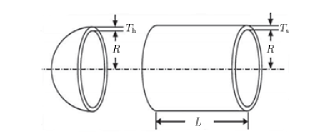
Figure 1: A diagram showing the design parameters of a pressure vessel fastf .

Algorithm 4 Algorithm for $P_{\Omega}(\mathbf{x}=[x_{1},x_{2},x_{3},x_{4}]^{\text{T}})$ in the pressure vessel problem

  $y_{1}=round(x_{1}/0.0625)\times 0.0625$

  if $y_{1}<0.0625$ then

     $y_{1}=0.0625$

  end if

  if $y_{1}>99\times 0.0625$ then

     $y_{1}=99\times 0.0625$

  end if

  $y_{2}=round(x_{2}/0.0625)\times 0.0625$

  if $y_{2}<0.0625$ then

     $y_{2}=0.0625$

  end if

  if $y_{2}>99\times 0.0625$ then

     $y_{2}=99\times 0.0625$

  end if

  if $x_{3}<10$ then

     $y_{3}=10$

  end if

  if $x_{3}>200$ then

     $y_{3}=200$

  end if

  if $x_{4}<10$ then

     $y_{4}=10$

  end if

  if $x_{4}>200$ then

     $y_{4}=200$

  end if

  return  $\mathbf{y}=[y_{1},y_{2},y_{3},y_{4}]^{\text{T}}$

Table 1: Comparisons of best results for the pressure vessel problem

	$x_{1}$	$x_{2}$	$x_{3}$	$x_{4}$	$g_{1}(\mathbf{x})$	$g_{2}(\mathbf{x})$	$g_{3}(\mathbf{x})$	$g_{4}(\mathbf{x})$	$f(\mathbf{x})$
csaam	0.8125	0.4375	42.0984	176.6366	8.00e-11${\dagger}$	-0.0359	-2.724e-4	-63.3634	6059.7143
fastf	0.7782	0.3846	40.3196	200.000	-3.172e-5	4.8984e-5${\dagger}$	1.3312${\dagger}$	-40	5885.33
aipso	0.8125	0.4375	42.0984	176.6366	8.00e-11${\dagger}$	-0.0359	-2.724e-4	-63.3634	6059.7143
anmha	1.125	0.625	58.2789	43.7549	-0.0002	-0.06902	-3.71629	-196.245	7198.433
niadp	1.125	0.625	48.97	106.72	-0.1799	-0.1578	97.760	-132.28	7980.894
gafnm	1.125	0.625	58.1978	44.2930	-0.00178	-0.06979	-974.3	-195.707	7207.494
uoasa	0.8125	0.4375	40.3239	200.0000	-0.034324	-0.05285	-27.10585	-40.0000	6288.7445
genas	0.9375	0.5000	48.3290	112.6790	-0.0048	-0.0389	-3652.877	-127.3210	6410.3811
aalmb	1.125	0.625	58.291	43.690	0.000016	-0.0689	-21.2201	-196.3100	7198.0428
asbsm	0.8125	0.4375	41.9768	182.2845	-0.0023	-0.0370	-22888.07	-57.7155	6171.000
gofsd	1.000	0.625	51.000	91.000	-0.0157	-0.1385	-3233.916	-149	7079.037
hagaw	0.8125	0.4375	42.0870	176.7791	-2.210e-4	-0.03599	-3.51084	-63.2208	6061.1229
agafn	1	0.625	51.2519	90.9913	-1.011	-0.136	-18759.75	-149.009	7172.300
aiaco	0.8125	0.4375	42.0984	176.6378	-8.8000e-7	-0.0359	-3.5586	-63.3622	6059.7258
PSA	0.8125	0.4375	42.0952	176.8095	-6.2625e-5	-0.0359	-738.7348	-63.1905	6063.2118

• ${\dagger}$ means that the corresponding constraint is violated.

In this subsection, the pressure vessel problem is considered. The pressure vessel problem is to find a set of four design parameters, which are demonstrated in Fig. 1, to minimize the total cost of a pressure vessel considering the cost of material, forming and welding 1 . The four design parameters are the inner radius $R$, and the length $L$ of the cylindrical section, the thickness $T_{\text{h}}$ of the head, the thickness $T_{\text{s}}$ of the body. Note that, $T_{\text{s}}$ and $T_{\text{h}}$ are integer multiples of 0.0625 in., and R and $L$ are continuous variables.

Let $\mathbf{x}=[x_{1},x_{2},x_{3},x_{4}]^{\text{T}}=[T_{\text{s}},T_{\text{h}},R,L]^{\text{T}}$. The pressure vessel problem can be formulated as follows fastf :

$$\text{minimize}\leavevmode\nobreak\ f(\mathbf{x}) =0.6224x_{1}x_{3}x_{4}+1.7781x_{2}x^{2}_{3}$$

$$\leavevmode\nobreak\ \leavevmode\nobreak\ +3.1661x^{2}_{1}x_{4}+19.84x^{2}_{1}x_{3},$$

$$\text{subject to}\leavevmode\nobreak\ g_{1}(\mathbf{x}) =-x_{1}+0.0193x_{3}\leq 0,$$

$$g_{2}(\mathbf{x}) =-x_{2}+0.00954x_{3}\leq 0,$$

$$g_{3}(\mathbf{x}) =-\pi x^{2}_{3}x_{4}-\frac{4}{3}\pi x^{3}_{3}+1296000\leq 0,$$

$$g_{4}(\mathbf{x}) =x_{4}-240\leq 0,$$

$$x_{1} \in\{1,2,3,\cdots,99\}\times 0.0625,$$

$$x_{2} \in\{1,2,3,\cdots,99\}\times 0.0625,$$

$$x_{3} \in[10,200],$$

$$x_{4} \in[10,200].$$

Evidently, this problem has a nonlinear cost function, three linear and one nonlinear inequality constraints. Besides, there are two discrete and two continuous design variables. Thus, the problem is relatively complicated. As this problem is a mixed discrete-continuous optimization, the projection function $P_{\Omega}(\mathbf{x})$ is slightly modified and presented in Algorithm 4. Besides, the initialization of the initial positions of porcellio scaber is modified as follows:

$${x}^{0}_{i,1} =0.0625+{floor}((99-1)\times{rand})\times 0.0625,$$

$${x}^{0}_{i,2} =0.0625+{floor}((99-1)\times{rand})\times 0.0625,$$

$${x}^{0}_{i,3} =10+{floor}(200-10)\times{rand},$$

$${x}^{0}_{i,4} =10+{floor}(200-10)\times{rand},$$

where ${x}^{0}_{i,j}$ denotes the $j$th variable of the position vector of the $i$th porcellio scaber; ${floor}(y)=\text{arg}\text{min}_{x\in\{0,1,2,\cdots\}}\{x+1>y\}$, i.e., the ${floor}$ function obtains the integer part of a real number; ${rand}$ denotes a random number in the region $(0,1)$. The functions ${floor}$ and ${rand}$ are available at Matlab.

The best result we obtained using the PSA in 1000 instances of executions and those by using various existing algorithms or methods for solving this problem are listed in Table 1. Note that, in the experiments, 40 porcellio scaber are used, the parameter $\lambda$ is set to 0.6, and the $MaxStep$ is set to 100000 with $\tau$ being a zero-mean random number with the standard deviation being 0.1. As seen from Table 1, the best result obtained by using the PSA is better than most of the existing results. Besides, the difference between the best function value among all the ones in the table and the best function value obtained via using the PSA is quite small.

Table 2: Comparisons of best results for Himmelblau’s nonlinear optimization problem

	$x_{1}$	$x_{2}$	$x_{3}$	$x_{4}$	$x_{5}$	$g_{1}(\mathbf{x})$	$g_{2}(\mathbf{x})$	$g_{3}(\mathbf{x})$	$f(\mathbf{x})$
couc	78.0	33.0	27.07997	45.0	44.9692	92.0000	100.4048	20.0000	-31025.5602
covga	78.00	33.00	29.995	45.00	36.776	90.7147	98.8405	19.9999${\dagger}$	-30665.6088
gaaed	81.4900	34.0900	31.2400	42.2000	34.3700	90.5225	99.3188	20.0604	-30183.576
anlp	78.6200	33.4400	31.0700	44.1800	35.2200	90.5208	98.8929	20.1316	-30373.949
mveob	78.00	33.00	29.995256	45.00	36.775813	92	98.8405	20	-30665.54
PSA	79.9377	33.8881	28.5029	41.3052	41.7704	91.6157	100.4943	20.0055	-30667.8113

• ${\dagger}$ means that the corresponding constraint is violated.

4.2 Case II: Himmelblau’s nonlinear optimization problem

In this subsection, we consider a nonlinear optimization problem proposed by Himmelblau anlp . This problem is also one of the well known benchmark problems for bio-inspired algorithms. The problem is formally described as follows anlp :

$$\text{minimize}\leavevmode\nobreak\ f(\mathbf{x})= 5.3578547x^{2}_{3}+0.8356891x_{1}x_{5}$$

$$+37.29329x_{1}-40792.141,$$

$$\text{subject to}\leavevmode\nobreak\ g_{1}(\mathbf{x})= 85.334407+0.0056858x_{2}x_{5}$$

$$+0.00026x_{1}x_{4}-0.0022053x_{3}x_{5},$$

$$g_{2}(\mathbf{x})= 80.51249+0.0071317x_{2}x_{5}$$

$$+0.0029955x_{1}x_{2}+0.0021813x^{2}_{3},$$

$$g_{3}(\mathbf{x})= 9.300961+0.0047026x_{3}x_{5}$$

$$+0.0012547x_{1}x_{3}+0.0019085x_{3}x_{4},$$

$$0\leq g_{1}(\mathbf{x})\leq 92,$$

$$90\leq g_{2}(\mathbf{x})\leq 110,$$

$$20\leq g_{3}(\mathbf{x})\leq 25,$$

$$78\leq x_{1}\leq 102,$$

$$33\leq x_{2}\leq 45,$$

$$27\leq x_{3}\leq 45,$$

$$27\leq x_{4}\leq 45,$$

$$27\leq x_{5}\leq 45,$$

with $\mathbf{x}=[x_{1},x_{2},x_{3},x_{4},x_{5}]^{\text{T}}$ being the decision vector. In this problem, each double-side nonlinear inequality can be represented by two single-side nonlinear inequality constraints. For example, the constraint $90\leq g_{2}(\mathbf{x})\leq 110$ can be replaced by the following two constraints:

$$-g_{2}(\mathbf{x}) \leq-90,$$

$$g_{2}(\mathbf{x}) \leq 110.$$

Thus, this problem can also be solved by the PSA proposed in this paper.

The best result we obtained via using the PSA in 1000 instances of executions, together with the result obtained by other algorithms or methods, is listed in Table 2. In the experiments, 40 porcellio scaber are used, the parameter $\lambda$ is set to 0.6, and the $MaxStep$ is set to 100000 with $\tau$ being a zero-mean random number with the standard deviation being 0.1. Evidently, the best result generated by the PSA is ranked No. 2 among all the results in Table 2.

By the above results, we conclude that the PSA is a relatively promising algorithm for solving constrained optimization problems. The quite smalle performance difference between the PSA and the best one may be the result of the usage of the penalty method with a constant penalty parameter.

5 Conclusions

In this paper, the bio-inspired algorithm PSA has been extended to solve nonlinear constrained optimization problems by using the penalty method. Case studies have validated the efficacy and superiority of the resultant PSA. The results have indicated that the PSA is a promising algorithm for solving constraint optimization problems. There are several issues that requires further investigation, e.g., how to select a best penalty parameter that not only guarantees the compliance with constraints but also the optimality of the obtained solution. Besides, how to enhance the efficiency of the PSA is also worth investigating.

References

- (1) J. Kennedy and R. Eberhart, “Particle swarm optimization,” in Proc. IEEE Int. Conf. Neural Netw., 1995, 1942–1948.
- (2) A. H. Gandomi, X. Y. Yang, “Benchmark problems in structural optimization,” in Computational Optimization Methods And Algorithms, Berlin: Springer-Verlag, 2011, pp. 259–281.
- (3) S. He , E. Prempain, and Q. H. Wu, “An improved particle swarm optimizer for mechanical design optimization problems,” Eng. Opt., vol. 36, no. 5, pp. 585–605, 2004.
- (4) A. H. Gandomi, X. S. Yang, and A. H. Alavi, “Cuckoo search algorithm: A metaheuristic approach to solve structural optimization problems,” Eng. Comput., vol. 29, pp. 17–35, 2013.
- (5) O. Pauline, H. C. Sin, D. D. C. V. Sheng, S. C. Kiong, and O. K. M., “Design optimization of structural engineering problems using adaptive cuckoo search algorithm,” in Proc. 3rd Int. Conf. Control Autom. Robot., 2017, pp. 745–748.
- (6) V. Garg and K. Deep, “Effectiveness of constrained laplacian biogeography based optimization for solving structural engineering design problems,” in Proc. 6th Int. Conf. Soft. Comput. Problem Solv., 2017, pp. 206–219.
- (7) D. Himmelblau, Applied Nonlinear Programming, New York: McGraw-Hill, 1972.
- (8) Y. Zhang and S. Li, “PSA: A novel optimization algorithm based on survival rules of porcellio scaber,” Available at https://arxiv.org/abs/1709.09840.
- (9) X. S. Yang, “Firefly algorithm, stochastic test functions and design optimisation,” Int. J. Bio-Inspired Comp., vol. 2, no. 2, pp. 2, pp. 78–84, 2010.
- (10) K. S. Lee and Z. W. Geem, “A new meta-heuristic algorithm for continuous engineering optimization: Harmony search theory and practice,” Comput. Methods Appl. Mech. Engrg., vol. 194, pp. 3902–3933, 2005.
- (11) E. Sandgren, “Nonlinear integer and discrete programming in mechanical design optimization,” J. Mech. Des. ASME, vol. 112, 223–229, 1990.
- (12) S. J. Wu and P. T. Chow, “Genetic algorithms for nonlinear mixed discrete-integer optimization problems via meta-genetic parameter optimization,” Engrg. Optim., vol. 24, 137–159, 1995.
- (13) C. A. C. Coello, “Use of a self-adaptive penalty approach for engineering optimization problems,” Comput. Ind., vol. 41, no. 2, pp. 113–127, 2000.
- (14) K. Deb, “GeneAS: a robust optimal design technique for mechanical component design”, in: D. Dasgupta, Z. Michalewicz Eds., Evolutionary Algorithms in Engineering Applications, Springer-Verlag, Berlin, 1997, pp. 497–514.
- (15) B. K. Kannan and S. N. Kramer, “An augmented Lagrange multiplier based method for mixed integer discrete continuous optimization and its applications to mechanical design,” J. Mecha. Design, Trans. ASME, vol. 116, pp. 318–320, 1994.
- (16) S. Akhtar, K. Tai, T. Ray, “A socio-behavioural simulation model for engineering design optimization,” Eng. Optmiz., vol. 34, no. 4, pp. 341–354, 2002.
- (17) J. F. Tsai, H. L. Li, and N. Z. Hu, “Global optimization for signomial discrete programming problems in engineering design,” Eng. Optmiz. no. 34, no. 6, pp. 613–622, 2002.
- (18) C. A. C. Coello and N. C. Corteś, “Hybridizing a genetic algorithm with an artificial immune system for global optimization,” Eng. Optmiz., vol. 36, no. 5, pp. 607–634, 2004.
- (19) H. L. Li and C. T. Chou, “A global approach for nonlinear mixed discrete programming in design optimization,” Eng. Optmiz. vol. 22, pp. 109–122 1994.
- (20) A. Kaveh and S. Talatahari, “An improved ant colony optimization for constrained engineering design problems,” Eng. Comput. vol. 27, no. 1, pp. 155–182, 2010.
- (21) G. H. M. Omran and A. Salman, “Constrained optimization using CODEQ,” Chaos Soliton. Fract., vol. 42, pp. 662–668, 2009.
- (22) A. Homaifar, S. Lai, X. Qi, “Constrained optimization via genetic algorithms,” Simulation, vol. 62, no. 4, pp. 242–253, 1994.
- (23) M. Gen and R. Cheng, Genetic Algorithms and Engineering Design, Wiley, New York, 1997.
- (24) G. G. Dimopoulos, “Mixed-variable engineering optimization based on evolutionary and social metaphors,” Comput. Method. Appl. Mech. Eng., vol. 196, pp. 803–817, 2007.