On the incidence of Mg ii absorbers along the blazar sightlines

Abstract

It is widely believed that the cool gas clouds traced by Mg ii absorption, within a velocity offset of 5000 kms^-1 relative to the background quasar are mostly associated with the quasar itself, whereas the absorbers seen at larger velocity offsets towards us are intervening absorber systems and hence their existence is completely independent of the background quasar. Recent evidence by Bergeron et al. (2011, hereinafter BBM) has seriously questioned this paradigm, by showing that the number density of intervening Mg ii absorbers towards the 45 blazars in their sample is nearly 2 times the expectation based on the Mg ii absorption systems seen towards normal QSOs. Given its serious implications, it becomes important to revisit this finding, by enlarging the blazar sample and subjecting it to an independent analysis. Here, we first report the outcome of our re-analysis of the available spectroscopic data for the BBM sample itself. Our analysis of the BBM sample reproduces their claimed factor of 2 excess of $dN/dz$ along blazar sightlines, vis-a-vis normal QSOs. We have also assembled a $\sim$3 times larger sample of blazars, albeit with moderately sensitive optical spectra. Using this sample together with the BBM sample, our analysis shows that the $dN/dz$ of the Mg ii absorbers statistically matches that known for normal QSO sightlines. Further, the analysis indicates that associated absorbers might be contributing significantly to the estimated $dN/dz$ upto offset speeds $\Delta v\sim 0.2c$ relative to the blazar.

1 Introduction

Analysis of the narrow absorption-line systems (in the spectra of quasars) has emerged as a powerful probe of the physical conditions of the gaseous medium of intervening galaxies, particularly when they lie at extremely large distances and hence too faint for direct imaging/spectroscopy even with the largest telescopes (Bahcall & Salpeter, 1966; Wolfe et al., 2005; Kulkarni et al., 2012). It is widely held that the cool gas clouds (e.g., Mg ii absorption systems) with velocities offsets $\beta$c up to $\sim$ 5000 km s^-1 relative to the background quasar are gravitationally bound to the quasar itself (i.e., ‘associated systems’, see Anderson et al., 1987; Khare et al., 1989; Møller et al., 1994, and references therein), whereas absorbers showing larger velocity offsets directed towards us are intervening systems probably associated with foreground galaxies and, consequently, their existence should be totally independent of the background quasar. A few recent studies, however, seem to question this canonical view, based on the differing estimates for the incidence rates of intervening systems (like Mg ii absorption having $\beta c\geq 5000$ km s^-1) detected towards different types of background sources, such as normal QSOs, gamma-ray bursters (GRBs) and blazars (Stocke & Rector, 1997; Prochter et al., 2006; Sudilovsky et al., 2007; Vergani et al., 2009; Tejos et al., 2009; Bergeron et al., 2011, hereinafter BBM). It has been also claimed by BBM and Cucchiara et al. (2009) that associated systems having a significantly relativistic speed relative to the quasar may also be present (BBM), e.g., when the quasar is undergoing powerful jet activity and/or ejecting high speed accretion-disk outflows. A possible way to differentiate between these possibilities would be to check if the incidence rates, $dN/dz$, of intervening absorbers differ depending on whether the background sources are non-blazars, or blazars whose powerful relativistic jets are therefore expected to be pointed close to our direction and, consequently the jet-accelerated potential absorbers would lie along the line-of-sight. Indeed, this expectation is echoed in the unexpected finding of BBM that the $dN/dz$ of Mg ii absorption systems (for strong absorbers having a rest-frame equivalent width W${}_{r}~{}\geq$ 1 Å) towards blazars is $\sim$ 2 times larger (at 3$\sigma$ confidence) than the value established for the sightlines to normal quasars (QSOs). An even greater excess had earlier been reported by Stocke & Rector (1997), albeit using a much smaller sample of blazars. On the other hand, a recent analysis by Chand & Gopal-Krishna (2012) of the existing high-resolution spectra of a sample of about 115 flat-spectrum radio-loud quasars (FSRQs, of non-blazar type) did not show any excess in the incidence of Mg ii absorption systems, as compared to QSOs. They reconciled the two seemingly discrepant results by appealing to the jet orientation scenario which lies at the heart of the Unified Scheme for powerful extragalactic radio sources (e.g. see, Antonucci, 1993). In their explanation, since the jets in FSRQs are thought to be less closely aligned to the line-of-sight, any gas clouds accelerated outward by the powerful jets are unlikely to appear in the foreground of the quasar’s nucleus and hence escape being detected in absorption against its bright optical emission. Later, Joshi et al. (2013) extended this probe by analyzing a large set of redshift-matched sightlines to 3975 radio core-dominated (CDQs, i.e., FSRQs) and 1583 radio lobe-dominated (LDQs) quasars. While, overall, only a marginal (9% at 1.5$\sigma$ significance) excess of $dN/dz$ was found towards the FSRQ sightlines, as compared to the sightlines to normal QSOs, they showed that the excess becomes quite significant (3.75$\sigma$) when the comparison is restricted to the absorbers having offset speeds i.e., $\beta<0.1c$ relative to the background quasar. Similarly, Tombesi et al. (2011) have used observations of Fe XXV/XXVI K-shell resonance lines in the X-ray band and found their outflow velocity distribution spans from $\sim$ 10,000 kms^-1 up to $\sim$ 100,000 kms^-1 ($\sim$ 0.3c), with a peak and mean value of $\sim$ 42,000 kms^-1 ($\sim$ 0.14c), for highly ionised gas clouds with column densities of N${}_{H}\approx$ 10²³ cm^-2 located within the central parsec of the AGN.

In this context, it is important to emphasize that even though BBM’s analysis has employed very high-sensitivity spectral data, their result rests on just 45 blazars, due to which small number statistics might be at work. It is worthwhile recalling that the 4-fold excess of $dN/dz$ along the GRB sightlines, inferred by Prochter et al. (2006) using just 14 GRBs, has subsequently been pronounced as a possible statistical fluke, on the basis of a 3 times larger set of sightlines (Cucchiara et al., 2013). Given its potentially deep ramifications, it is therefore desirable to revisit the BBM claim of excess $dN/dz$ towards blazars, by enlarging the blazar sample and carrying out an independent analysis. The present study is motivated by this objective.
The paper is organized as follows, in Section 2 we describe our sample, while in Section 3 our data analysis procedure is outlined. The results are given in Section 4, followed by a brief discussion and conclusions in Section 5.

2 The Sample

Table 1: The spectral data sourcing for our enlarged sample of blazars.

Archive	Instrument	Content	Resolution
ESO	FORS-1/2	48 blazars found (10 taken)	900
ESO	X-SHOOTER	17 found(8 taken)	3600
ESO	UVES	1 found (taken)	40000
SAO	SCORPIO	3 new observations (3 taken)	818
KECK	LRIS	2 (both taken)	9800
SDSS	BOSS	622 found (196 taken)	2500
BBM	FORS-1	42 (all 42 taken)	900

The blazar sample employed in our analysis is an amalgamation of 3 sets of blazars extracted from the catalogues published by Massaro et al. (2009, hereafter ROMA-BZCAT), Véron-Cetty & Véron (2010, hereafter VV), and Padovani & Giommi (1995, hereafter, Padovani-Catalogue). From the ROMA-BZCAT we selected sources classified as BZB (implying confirmed BL Lac), resulting in a set of 1059 blazars. From the VV catalogue we selected the sources classified either as ‘BL’ (i.e., confirmed BL Lac), or ‘HP’ (a confirmed highly polarized quasar). This resulted in a set of 729 confirmed blazars from this catalogue. Accounting for the 480 sources that are common to these two sets, led to a list of 1308 confirmed blazars. The Padovani-catalogue also classifies BL Lacs objects using homogeneous criteria. It contains a total of 233 blazars, of which 189 were already in the above two sets (among them 169 blazars of the Padovani-catalogue are in BZ-ROMA, while 20 in the VV catalogue). Their exclusion left us with 44 blazars solely contributed by the Padovani-catalogue. Merging these 3 sets resulted in our final ‘parent sample’ of 1352 confirmed blazars.

We then performed an extensive search for optical spectra of our parent sample of blazars, in the archives of the Sloan Digital Sky Survey (SDSS), the European Southern Observatory (ESO) and the KECK Observatory. We applied two main selection filters: (i) median SNR of the entire spectrum should be more than 5, so that false detections of Mg ii line are minimized, and (ii) the blazar’s redshift should allow at least $10\times(1+z_{em}$)Å  wide coverage in the available spectrum, of the region between the Ly$\alpha$ and Mg ii emission lines; this would ensure that the observed spectrum can be used to search for the Mg ii doublet due to at least one absorber (given that the two components of the doublet Mg ii $\lambda$ 2796, 2803, are separated by 8 Å  in the rest frame).

In the ESO archive, after excluding the spectra of the 42 BBM blazars, which had been taken using the FOcal Reducer and the low-dispersion Spectrograph (FORS1) at the ESO observatory, we found that for 66 of our blazars (within 1 arcmin search radius) a spectrum with SNR $>5$ was available either in the reduced form, from the ESO-advanced data product (17 observed using X-shooter spectrograph, 1 observed using the Ultraviolet and the Visual Echelle Spectrograph (UVES) ), or we were at least able to extract the spectra based on their raw images using associated calibration files (48 observed using FORS-1,2). Among these 66 blazars, emission redshift was available for only 31, out of which just 16 were found useful for Mg ii  absorber search after applying our emission redshift constraint mentioned above. For the remaining 35 blazars with unknown emission redshifts we could establish a lower redshift limit for 4 blazars using the redshift of the observed most redshifted Mg ii  absorption doublet. One of these 4 had to be excluded as the Mg ii  derived redshift was not yielding adequate redshift path (i.e., not satisfying the selection criteria-ii). Here, it is also important to clarify that the spectral region containing this most redshifted absorption doublet was excluded for the purpose of computing $dN/dz$, in order to keep the estimate free of bias resulting from exclusion of those blazars with unknown redshift, for which even a lower limit to redshift could not be established (using the Mg ii absorption doublet).

For another three blazars from our ‘parent-sample’ (see above), viz, J145127$+$635426, J165248$+$363212, J182406$+$565100, we have newly obtained spectra using the SCORPIO spectrograph (using VPHG1200 grism) mounted on the 6-m telescope at the Special Astrophysical Observatory (SAO). Inclusion of another 2 blazars viz, J001937$+$202146, J043337$+$290555, became possible due to the availability of their spectra in the KECK archive, taken with the Low Resolution Imaging Spectrometer (LRIS).

For 622 blazars in our ‘parent sample’ we could find spectra in the SDSS archives (within a tolerance of 2 arcsec) in reduced form, covering a wavelength range 3800-10000Å. Excluding the 69 spectra with SNR $<5$, left us with good quality spectra for 553 blazars. Among these, emission redshifts were available for 277 blazars, out of which 150 sources were found useful for Mg ii  absorber search, after meeting our aforementioned emission redshift criterion (selection criterion-ii). In addition, from among the 276 blazars with unknown emission redshift, a lower redshift limit could be set for 59 sources, using the detected Mg ii  absorption feature. However, one of these 59 sources (viz, J130008.5$+$175538) had to be excluded as it did not meet our criterion of useful minimum redshift path (i.e., the selection criterion-ii). In addition, after excluding another 12 blazars as they are already included in our above sample from other resources (ESO archive and SAO observations) we are left with 196 blazars solely contributed by the SDSS, which are found satisfactory for the purpose of our Mg ii  absorption-line search.

To recapitulate, we have assembled a sample of 220 blazars (SDSS: 196, ESO: 19, SAO: 3, KECK: 2) as summarized in Table 1, to make a search for intervening Mg ii  absorbers. Out of these, only a lower limit to $z_{em}$ is available for 58 blazars (i.e. 54 SDSS, 3 ESO and 1 KECK). We have dicussed three out of them in Appendix A where we have also shown their represtative spectra as well.

Further, as mentioned above, we have also made use of the BBM blazar sample to revisit their conclusion (section 1), by subjecting it to an independent data reduction and analysis procedure, as followed in the present work. The sample employed in their analysis consists of 45 blazars. For 42 of them, we could obtain the raw spectral data from the ESO archive based on their program ID 080:A-0276, 081:A-0193. The raw data used in the BBM analysis for the remaining 3 (northern sky) blazars were not accessible and hence they could not be included in our analysis.

The $z_{em}$ and SNR distributions for our sample of 262 blazars (including 42 from the BBM sample) are shown in Fig. 1. However, as described in Section 3.2, among the 220 non-BBM blazars only 149 blazars were found to contribute to robust redshift path for the case of strong absorbers and only 58 of them have contributed to the robust redshift path for weak absorbers, as well. Thus, for the purpose of the present $dN/dz$ analysis, we are led to a final sample of 191 blazars (149 ours plus 42 BBM blazars) for the strong absorber case. Only 100 out of them also contribute to the $dN/dz$ analysis for weak absorbers. The sample of 191 blazars is listed in Table LABEL:table:full_sample.

Table 2: Basic properties of our sample of 191 blazars.

Target	$z_{em}$	Data archive	$\Delta$z${}_{strong}^{a}$	SNR
J001937$+$202146	0.858	KECK	0.417	6.4
J003514$+$151504	0.443	SDSS	0.123	55.0
J003808$+$001336	0.740	FORS/ESO	0.439	91.8
J004054$-$091525	5.030	FORS/ESO	0.891	66.2
—	—	—	—	—–
Note. The entire table is available in on-line version. Only a
portion of this table is shown here, to display its form and content.
aThe redshift path contribution to the strong Mg ii system
(W${}_{r}(2796)\geq 1.0$ Å) analysis.

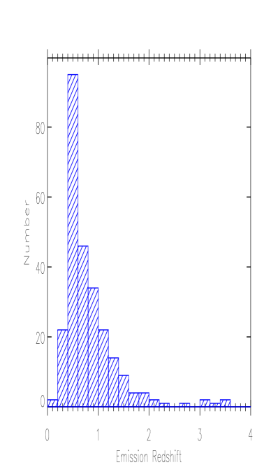
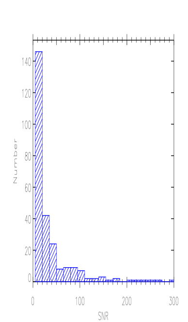
Figure 1: Distributions of emission redshift (left) and SNR (right) for our full sample of 262 blazars (including the​ ​ 71 blazars which are subsequently excluded from the Mg ii strong systems analysis; see Section 3.2. For 58 blazars without exact $z_{em}$, we have used their lower limit on $z_{em}$, derived based on the most redshifted absorption system seen in their spectra).

3 Analysis

3.1 Data Reduction

Data reduction for the FORS spectra available for our 53 blazars, including the 42 blazars from BBM, was performed using the ESO-FORS pipeline (version 5.1.4), by executing it using the ESOREX algorithm. The pipeline performs a precise background subtraction on science frames, does master flat-fielding, rejects cosmic-ray impacts by employing an optimal extraction technique and then applies calibrations for wavelength and flux. The Keck/LRIS data were reduced using a publicly available Lris automated reduction Pipeline (lpipe) written in idl. The UVES and SDSS spectra (total 197 blazars) were already available in the reduced form. Finally, the spectra taken with the SAO 6-m telescope for 3 of our blazars (viz, J145127$+$635426, J165248$+$363212 and J182406$+$565100) were reduced using the standard IRAF tasks. For post-processing of each one-dimensional spectrum, which involves steps such as air-to-vacuum wavelength conversion, heliocentric correction, combining individual exposures for SNR enhancement and continuum fitting to determine the normalized spectrum, we have followed the procedure described in Chand et al. (2004).

3.2 Computation of the EW detection limit and the corresponding useful redshift path

For identifying absorption features in a given spectrum, proper evaluation of noise plays a crucial role as it defines the detection limit for the features. Therefore, to generate the distribution of rms noise along the spectrum we used the matched-filtering technique employed by Zhu & Ménard (2013), which involves the following main steps:
(i) Subtracting unity from each point/pixel of the normalized spectrum (thus, the mean level of the spectrum becomes zero).
(ii) Using this residual spectrum, generate its amplitude version, by plotting only the magnitude of the signal at each spectral pixel (i.e., setting the negative sign to positive).
(iii) This ‘noise amplitude spectrum’ is then subjected to a top-hat smoothing over the ‘effective spectral resolution’, which is taken to be the quadratic sum of the instrumental resolution and the typical Mg ii absorption line width. For instance, the typical FWHM of the QSOs absorption line convolved with the SDSS instrumental resolution lies in the range $\sim$ 100-400 kms^-1 ($\sim$ 2-6 pixels). Thus, for the SDSS instrumental resolution of 120 kms^-1, we have taken an ‘effective spectral resolution’ of about 4 pixels (i.e., $\sim$ 276 kms^-1, e.g., see Zhu & Ménard, 2013).
(iv) This ‘smoothed noise amplitude spectrum’ was then sub-divided into a sequence of 100 Å  wide segments. Within each segment all points deviating by more than one $\sigma$ were clipped (including any spectral lines) and substituted with interpolated values. In this smoothed noise amplitude spectrum the amplitude at a given spectral (i.e., wavelength) pixel ‘$i$’ is the representative noise, $n_{i}$, for that pixel.
(v) For each spectral pixel, we then set the 3$\sigma$ detection threshold of a spectral feature. To do this, we model the feature as a Gaussian having a FWHM equal to the afore-mentioned ‘effective spectral resolution’ and then subject it to the same ‘top-hat’ smoothing as mentioned in (iii) above, and finally, we optimize its amplitude to equal 3$n_{i}$. Equivalent width of the Gaussian satisfying this criterion thus becomes the limiting equivalent width ($W_{i,det}$) of the Mg ii absorption line that would be accepted as a significant (3$\sigma$) detection at that particular pixel in the spectrum. Only provided the pre-set restframe threshold value ($W_{th}$), which is 0.3 Å  for weak and 1.0 Å  for strong absorption systems, respectively, exceeds the computed $W_{i,det}$ for that pixel, would that spectral pixel be accepted as contributing to ‘useful’ redshift path, not otherwise. Note that this procedure is very similar to that adopted in Mathes et al. (2017).

As a result, for our blazar sample, the net useful redshift path at a given redshift $z_{i}$ (so that the Mg ii absorption line falls in the $i^{th}$ spectral pixel) for detection of the Mg ii doublet above a designated rest-frame equivalent width threshold, $W_{th}$ would be:

$$\begin{aligned} g\left(W_{th},z_{i}\right)&=\sum_{j=1}^{N_{blazar}}\ H(z_{i}-z_{j,min})\times H(z_{j,max}-z_{i})\\ &\times H(W_{th}-{W_{j,det}(z_{i})})\\ \end{aligned}$$ (1)

where $H$ is the Heaviside step function, and the summation is taken over all the blazar spectra in our sample, $z_{j,min}$ and $z_{j,max}$ are, respectively, the minimum and maximum expected absorption redshift limits which were used in the search for the Mg ii doublet for $j^{th}$ quasar (see Section 3.3). $W_{th}$ is the threshold rest-frame EW of the Mg ii absorption line which we have set at 1 Å  and 0.3 Å, for strong and weak absorption systems, respectively. $W_{j,det}(z_{i})$ is the computed rest-frame EW detection limit at the i^th pixel in the spectrum of the $j^{th}$ quasar, as discussed above. In the parent sample of 262 blazar, a non-zero $g\left(W_{th},z_{i}\right)$ was found for only 191 blazars for the strong absorber case, and 100 out of them also contributed a non-zero $g\left(W_{th},z_{i}\right)$ for the case of weak absorption system, as well. Hence only these two subsets have been used in the present $dN/dz$ analysis.

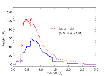
Figure 2: The distributions of redshift path density for the intervening Mg ii systems towards blazars, for the strong (W${}_{r}(2796)\geq 1.0$ Å: red dashed curve) and the weak absorption systems ($0.3\leq$ W${}_{r}(2796)<1.0$ Å: blue solid curve).

3.3 Mg ii absorption-line identification

Table 3: The detected 43 Mg ii absorption systems
and their rest-frame equivalent widths, W_r(Mg ii $\lambda 2796$ Å),
as identified in 34 blazars belonging to our sample of 191 blazars.

Blazar	$z_{em}$	$z_{abs}$	Wr	Associated absorptions
J001937$+$202146	0.858	0.69616	1.0969	Fe ii
J010009$-$333730	0.875	0.67996	0.5110	Fe ii
J014125$-$092843	0.730	0.50042	0.3641	Fe ii
J021748$+$014449	1.715	1.34428	2.0130	Mg i , Fe ii , Zn ii , Mn ii
J023838$+$163659	0.940	0.52379	2.3725	Mg i , Fe ii , Mn ii
—	—	—	—	—
Note. The entire table is available in the on-line version.
Only a portion of the table is shown here to display its form
and content.

Normally, the wavelength coverage may differ from spectrum to spectrum, as it depends on the spectrograph’s specifications and the instrumental settings used for the observations. Additionally, we place two constraints on the redshift path over which the search for the Mg ii doublet was made. Firstly, the search was restricted to within the range $(1+z_{em})\times 1216$Å  $<\lambda<(1+z_{em})\times 2803$Å. The lower limit is meant to avoid the Ly$\alpha$ forest, while the upper limit is dictated by the fact that any Mg ii absorber with $\lambda\geq(1+z_{em})\times 2803$Å  has a strong likelihood of being an associated system falling into the background AGN. We performed the search for the Mg ii doublet at $z_{em}$ following the steps enumerated in section 3 of Chand & Gopal-Krishna (2012). Accordingly, a line profile matching technique was used, such that we first plotted the normalized spectrum of a given blazar and then overplotted the same spectrum by shifting the wavelength axis by a factor of Mg ii $\lambda 2796.3543$/Mg ii $\lambda 2803.5315$ (i.e. 0.997). Then, about 50 Å  wide spectral segments were manually examined. The location of perfect overlap between the absorption lines in the shifted and the original (unshifted) spectra were marked as a detected Mg ii absorption system. As a further corroboration, we looked for the corresponding metal lines (e.g. Fe ii , C iv , Si ii , etc.) in the spectrum. If the redshift/velocity of a Mg ii absorption doublet was found to be consistent with that of the peak estimated for the metal line(s), this was taken as a further confirmation of the previously identified Mg ii absorber. Note that the systems having a velocity offset within 5000 kms^-1 of $z_{em}$ of the blazar were classified as associated systems, following the standard practice. For each detected Mg ii absorption system, we also performed visually a quality check on the fit to the underlying continuum. If deemed desirable we carried out a local continuum fitting and this improved fit was then used to obtain a better estimate of W_r(Mg ii ). Detailed information on the 43 Mg ii absorption systems thus identified in the spectra of 34 blazars, out of the total present sample of $191$ blazars, is provided in Table LABEL:table:mgii_absorbers.

3.4 Computation of $dN/dz$

The incidence rate of Mg ii absorbers is defined as $\frac{dN}{dz}=N_{obs}/\Delta z$; where $N_{obs}$ is the total number of the Mg ii absorbers detected within the entire useful redshift path ($\Delta z$), defined as:

$$\Delta z=\int_{0}^{\infty}\sum_{j=1}\ g_{j}(W_{min},z_{i})dz_{i}$$ (2)

where g${}_{j}(W_{min},z_{i})=1$ if W_th ( 0.3 Å  for weak systems and 1 Å  for strong systems) is more than the (3$\sigma$) detection threshold W${}_{j,det}(z_{j})$ estimated for the $i^{th}$ spectral pixel (see Eq. 1), otherwise $g(W_{min},z_{i})=0$. The values of redshift path density for $i^{th}$ redshift pixel, i.e., $g(W_{min},z_{i})$, were thus computed using the total 191 blazar sightlines for strong absorption systems and the 100 blazar sightlines for weak absorption systems (Fig. 2).

Table LABEL:table:full_sample lists the values of $\Delta z$ calculated for the individual sightline in our entire blazar sample and in its various sub-sets. The errors in the computed $dN/dz$ values were estimated assuming the Poisson small number statistics for $N_{obs}<50$, within a limit of 1$\sigma$ confidence level of a Gaussian distribution, using the tabulation given by Gehrels (1986).

4 Results

4.1 Incidence of Mg ii absorbers in the present enlarged sample

Table 4: Incidence of Mg ii absorbers for the present sample and its various subsets.

Sample type	Weak absorption systems				Strong absorption systems
	$N_{obs}$	$\Delta$z	$\frac{N_{obs}}{\Delta z}\equiv dN/dz$	$\left(\frac{(N_{obs}/\Delta z)}{(dN/dz)_{qso}}\right)^{\alpha}$	$N_{obs}$	$\Delta$z	$\frac{N_{obs}}{\Delta z}$	$\left(\frac{(N_{obs}/\Delta z)}{(dN/dz)_{qso}}\right)^{\beta}$
Sample I a	23	44.21	$0.52_{0.11}^{0.13}$	$1.21_{0.25}^{0.31}$	20	86.08	$0.23_{0.05}^{0.06}$	$1.26_{0.28}^{0.35}$
Sample II b	20	40.06	$0.50_{0.11}^{0.14}$	$1.16_{0.26}^{0.32}$	16	81.41	$0.20_{0.05}^{0.06}$	$1.07_{0.26}^{0.34}$
Sample III c	17	32.69	$0.52_{0.12}^{0.16}$	$1.20_{0.29}^{0.37}$	13	60.10	$0.22_{0.06}^{0.08}$	$1.11_{0.30}^{0.40}$
Sample IV d	6	19.05	$0.31_{0.12}^{0.19}$	$0.74_{0.29}^{0.44}$	8	58.98	$0.14_{0.05}^{0.07}$	$0.80_{0.28}^{0.39}$
Sample V e	3	11.69	$0.26_{0.14}^{0.25}$	$0.57_{0.31}^{0.56}$	5	37.67	$0.13_{0.06}^{0.09}$	$0.72_{0.31}^{0.49}$
Sample VI f	4	15.48	$0.26_{0.12}^{0.20}$	$0.59_{0.28}^{0.47}$	7	52.21	$0.13_{0.05}^{0.07}$	$0.76_{0.28}^{0.41}$
Sample VII g	2	9.29	$0.22_{0.14}^{0.28}$	$0.46_{0.29}^{0.60}$	5	32.70	$0.15_{0.07}^{0.10}$	$0.76_{0.33}^{0.51}$
Sample VIII h	16	24.58	$0.65_{0.16}^{0.21}$	$1.52_{0.38}^{0.48}$	9	29.20	$0.31_{0.10}^{0.14}$	$1.61_{0.53}^{0.73}$
Sample IX i	15	23.41	$0.64_{0.16}^{0.21}$	$1.50_{0.38}^{0.50}$	8	27.41	$0.29_{0.10}^{0.14}$	$1.52_{0.52}^{0.75}$
α $dN/dz$ for QSOs is calculated at the mean value of the redshift path of the blazars, using equation 2 of BBM.
β $dN/dz$ for QSOs is calculated at the mean value of the redshift path of the blazars, using equation 6 of BBM.
a Full sample of 191 blazars (also included are the sources with only a lower limit available for  $z_{em}$).
b 184 BL Lacs, i.e., Sample I (191 blazars) $-$ 7 (BBM FSRQs).
c 133 BL Lacs, i.e., Sample II ( 184 BL Lacs) $-$ 51 (sources with only a lower limit on $z_{em}$).
d 149 Non-BBM BL Lacs, i.e., Sample I (191 blazars) $-$ 42 (BBM blazars).
e 98 Non-BBM BL Lacs, i.e., Sample IV (149 Non-BBM BL Lacs) $-$ 51 (Non-BBM BL Lacs with only lower limit on $z_{em}$).
f 126 SDSS BL Lacs, i.e., Sample II (184 BL Lacs) $-$ 58 (Non-SDSS BL Lacs).
g 79 SDSS BL Lacs, i.e., Sample VI (126 SDSS BL Lacs) $-$ 47 (SDSS BL Lacs with only lower limit on $z_{em}$).
h 58 Non-SDSS BL Lacs, i.e., Sample II (184 BL Lacs) $-$ 126 (SDSS BL Lacs).
i54 Non-SDSS BL Lacs, i.e., Sample VIII (58 Non-SDSS BL Lacs) $-$ 4 (Non-SDSS BL Lacs with only lower limit on $z_{em}$).

Table 5: Incidence of strong Mg ii absorption systems
towards the low SNR (SNR$<$15) and high SNR ($>$15)
spectra in our sample of 191 blazars. The last column shows
the same relative to normal QSOs.

Sample type	$N_{obs}$	$\Delta$z	$\frac{N_{obs}}{\Delta z}$	$\left(\frac{(N_{obs}/\Delta z)}{(dN/dz)_{qso}}\right)^{\alpha}$
Low SNR	7	28.74	$0.24_{0.09}^{0.13}$	$1.19_{0.44}^{0.64}$
High SNR	13	57.33	$0.23_{0.06}^{0.08}$	$1.29_{0.35}^{0.47}$
${}^{\alpha}(dN/dz)_{qso}$ for the strong systems (W${}_{r}(2796)\geq 1.0$ Å) is calculated
(as done in BBM analysis) based on Prochter et al. (2006).

As noted in Section 1, the BBM result is based on a sample of just 45 blazars and this has motivated us to build an enlarged sample. Our sample of 191 blazars provides nearly a factor of 3 increase in the redshift path (Table LABEL:table:full_sample). Table 4 summarizes the results for this enlarged sample and its various subsets. Note that, as in BBM, the values of $dN/dz$ for normal QSOs are calculated at the mean value of the redshift path for the corresponding blazar subset (column 1 of Table 4). This was done using equation 2 of BBM for the case of weak absorption systems, and equation 6 of BBM, for the case of strong absorption systems. From Table 4, no significant excess is evident in the $dN/dz$ for the blazar sightlines, vis a vis normal QSOs, both for weak (column 5) and strong (column 9) Mg ii absorbers. The same is apparent from Fig. 3, which displays the cumulative numbers of Mg ii absorbers up to different values of absorption redshift. Although, when only the absorption systems having $\Delta v<5000$ kms^-1 are deemed as associated systems and therefore excluded, a mild excess may be present for blazar sightlines (Fig. 3 top panel). However, it vanishes for the strong systems if one excludes all absorbers having offset velocities up to $\Delta v<30000$ kms^-1 (Fig. 3 middle panel). The mild excess vanishes even for weak systems if the absorbers with offset velocities up to $\Delta v<60000$ kms^-1 are excluded (Fig. 3 bottom panel), suggesting the possibility of extension of Mg ii intrinsic absorbers up to $\Delta v$ = 0.2c for blazars. In any case, our focus here is on the results for strong absorption systems, which are statistically more robust since the majority of our spectra (which have relatively low SNR) have contributed to the useful redshift path only for strong systems and not for weak systems.

In Fig. 4 we have displayed the redshift dependence of $dN/dz$ for strong ($W_{\rm r}(\lambda 2796)\geq 1.0$ Å) Mg ii absorption systems detected in our blazar sample and compared it with that computed for the sightlines towards normal QSOs, using the analytical expression given by Zhu & Ménard (2013) for strong Mg ii absorption systems. To quantify the similarity of these two distributions we have applied Kolmogorov-Smirnov (KS) test, which resulted in P_null=0.997; where P_null is the null probability that two distributions are indistinguishable. Similarly a very good statistical agreement is found between the estimates of $dN/dz$ for blazars and QSOs, with a $\chi^{2}$-test giving P_null = 0.99, leading us to infer that the distributions of $dN/dz$ for blazars and QSOs are statistically indistinguishable. Recall that it is for the strong absorption systems that BBM had reported a significant excess of $dN/dz$ (compared to QSOs sightlines), based on the high SNR spectroscopic data available for their sample of 45 blazars. To pursue this further, we present in the next section a re-analysis of their data following our data reduction and analysis procedure. Since this has yielded results consistent with the BBM claim, could then the discrepant result we have found here using a much larger sample of blazars (Table 1) have its origin in the substantially lower SNR of the spectra available for most of the present enlarged sample? To check this possibility we divide our blazar sample into (i) a low SNR subset (spectra having SNR between 5 and 15) and (ii) a high SNR subset (SNR $\textgreater$ 15). It is seen from Table 5 that in neither case is a significant excess of $dN/dz$ (vis a vis normal QSOs) detected for the strong Mg ii absorption systems (the same is found to hold for the weak absorption systems as well ). Thus, the discrepant result found here for the present blazar sample from the BBM sample is unlikely to be on account of the SNR contrast between the spectral data employed in the two studies. An alternative possibility is explored in the next section.

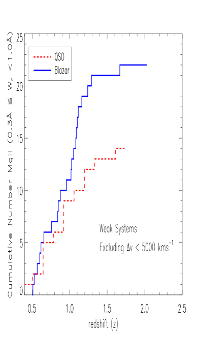
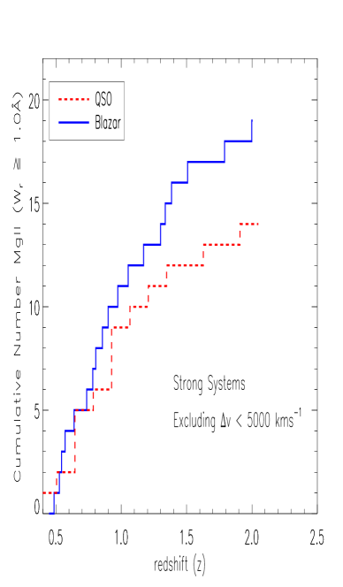
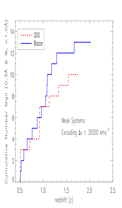
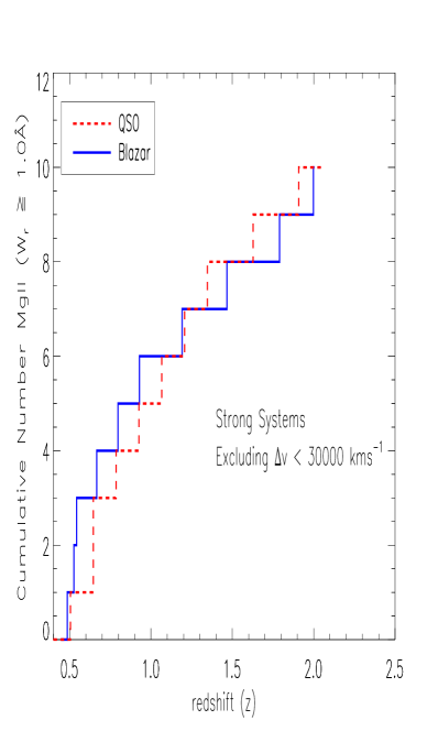
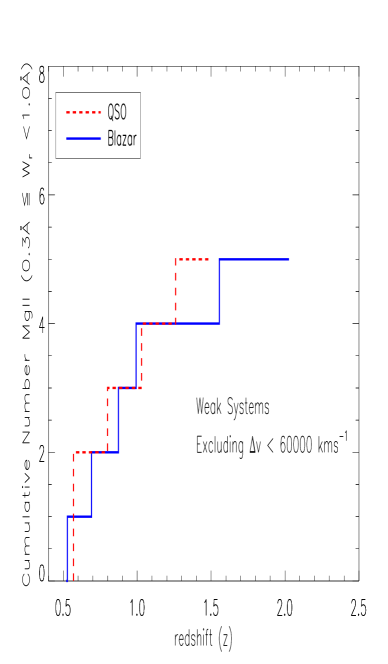
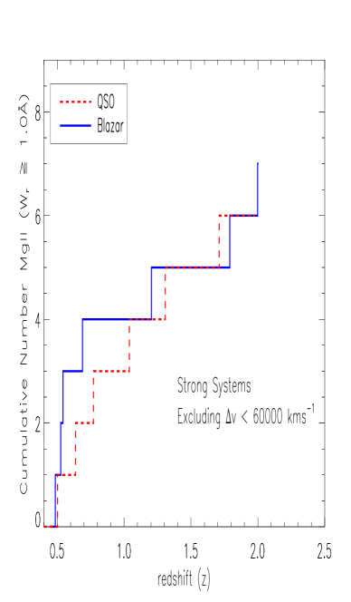
Figure 3: Cumulative number of weak (left) and strong (right) intervening Mg ii absorption systems detected towards blazars (blue solid line) and QSOs (red dashed line), after excluding the systems with offset velocity ($\Delta v$) $<5000$ kms^-1 (top panel), $\Delta v<30000$ kms^-1 (middle panel) and $\Delta v<60000$ kms^-1 (bottom panel). For QSOs the estimates for weak Mg ii systems are taken from Nestor et al. (2005) (see text), and for strong systems these are adopted from Prochter et al. (2006)

.

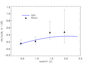
Figure 4: Number density evolution of strong (W${}_{\rm r}(2796)\geq 1.0$ Å) Mg ii absorption systems (averaged over redshift bins of 0.5) towards our 191 blazar sightlines (black triangles), and the sightlines towards the QSOs in the SDSS (blue solid line). The absorption systems with $\Delta v<5000$ kms^-1 have been excluded. The solid line for the SDSS QSOs has been computed from the analytical expression given by Zhu & Ménard (2013) for strong Mg ii absorption systems towards QSOs. The two distributions show an excellent agreement with a P_null of $\sim 0.99$ based on the KS and $\chi^{2}$ tests.

4.2 Re-analysis of the BBM sample

Table 6: Re-analysis of the (high sensitivity) spectra of the 42 southern blazars in the BBM sample.

Absorber type	W${}_{r}(2796)$-range	Nre-analysis	$\Delta$zre-analysis	NBBM	$\Delta z_{BBM}$	$\left(\frac{(dN/dz)_{re-analysis}}{(dN/dz)_{BBM}}\right)$
Strongγ	W${}_{r}\geq 1.0~{}$Å	12	27.10	12	28.04	$1.03\pm 0.48$
Strongβ	W${}_{r}\geq 1.0~{}$Å	8	22.44	10	23.44	$0.83\pm 0.46$
Weakγ	$~{}0.3~{}$Å$\leq$W${}_{r}<1.0$	17	25.16	19	25.11	$0.89\pm 0.33$
Weakβ	$~{}0.3~{}$Å$\leq$ W${}_{r}<1.0$	14	21.01	15	20.55	$0.91\pm 0.38$
γFor the 42 BBM blazars.
β Analysis using 35 BL Lacs in BBM sample. It is to be noted that out of the 42 blazar in BBM sampe,
32 were designated as BL Lacs. The other three included BL Lacs are those which in BBM sample were classified
as non-BL Lac (i.e ’opt’ class in BBM) viz, J023405$-$301519, J024156$+$004351, J221450$-$293225, but are reported
as confirmed BL Lacs in VV catalouge and hence are included here in this sample of 35 BL Lacs.

As discussed in Section 1, based on a sample of 45 blazars having high-sensitivity (ESO/FORS) spectra BBM found about a factor of 2 excess in the number density of Mg ii absorbers on the blazar sightlines, as compared to the sightlines to normal QSOs. Since the present analysis of a sample of 191 blazars does not show such a trend, we have carried out a re-analysis of the BBM sample using the same procedure which we have followed here for our sample. As mentioned in Section 2, we have limited the re-analysis to 42 out of the 45 BBM blazars, since we could not access the requisite raw spectral data for the remaining 3 (northern) blazars. For both weak and strong absorption systems, Table LABEL:Table:bbm_excess_netzor compares our results with the BBM estimates of $N_{obs}$, $\Delta z$ and $dN/dz$. It is clear that the BBM estimates are reasonably well reproduced in our analysis; a few minor discrepancies are noted below.

For strong systems, there is a small difference in the redshift path, our value of 27.1 is slightly lower than the BBM estimate of 28.04. This small difference might be owing to the difference in the methods of determining ‘useful’ redshift path. We also compared the absorption redshifts and equivalent widths of the detected Mg ii absorption systems and a good match was found, except in two cases: (i) the system at $z_{abs}$ = 0.5592 towards the blazar J0428$-$3756 was classified as ‘weak’ in BBM (W_r= 0.93), but ‘strong’ (W_r= 1.03) in our analysis, and (ii) the $z_{abs}$ = 1.1158 system towards J2031$+$1219 was classified as ‘strong’ (W_r= 1.29 ) in BBM, but ‘weak’ (W_r= 0.94) in our analysis. Coming to the weak systems, we detected a total of 17 Mg ii absorbers, whereas BBM reported 19 Mg ii absorbers, with the redshift path being 25.16 in our case, very close to their estimate of 25.11. Two systems, viz. (i) the $z_{abs}$ = 1.1039 system towards J1419$+$0445 (W_r= 0.52) and (ii) the $z_{abs}$ = 0.6236 system towards J1956$-$3225 (with W_r= 0.95), could not be included in our analysis. The former remained undetected and the latter system corresponds to a wavelength of 4539 Å which falls just below the starting wavelength of 4540 Å of the spectrum used in our analysis.

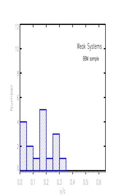
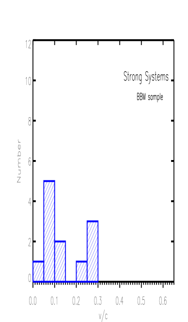
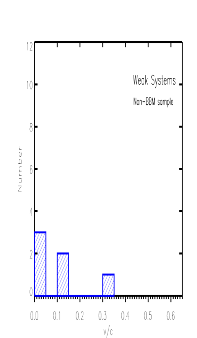
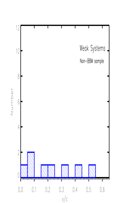
Figure 5: Top: Velocity distribution of the Mg ii absorbers, relative to the background blazar (Eq. 3) for the 17 weak $(0.3~{}\AA~{}\leq$W${}_{\rm r}(2796)<1.0$ Å ; left) and 12 strong ( W${}_{\rm r}(2796)\geq 1.0$ Å ; right) ‘intervening’ Mg ii absorbers seen towards the 42 BBM blazars, (see Section 4.2). Bottom: The same as the top panel for the 7 weak and 8 strong ‘intervening’ Mg ii absorbers detected towards 160 blazars (among which only 64 have useful redshift path for weak systems) after excluding the BBM blazars. Note that the absorption systems with offset velocities $\Delta v<5000$ kms^-1, i.e., $\beta<0.017$ have been excluded.

Table 7: The results for the present sample and its various subsets, after excluding the Mg ii absorption systems with $\Delta v<60000$ kms^-1.

Sample type†	Weak systems				Strong systems
	$N_{obs}$	$\Delta$z	$\frac{N_{obs}}{\Delta z}$	$\left(\frac{(N_{obs}/\Delta z)}{(dN/dz)_{qso}}\right)^{\alpha}$	$N_{obs}$	$\Delta$z	$\frac{N_{obs}}{\Delta z}$	$\left(\frac{(N_{obs}/\Delta z)}{(dN/dz)_{qso}}\right)^{\beta}$
Sample I	6	18.80	$0.32_{0.13}^{0.19}$	$0.76_{0.30}^{0.45}$	8	39.68	$0.20_{0.07}^{0.10}$	$1.10_{0.38}^{0.54}$
Sample II	5	16.87	$0.30_{0.13}^{0.20}$	$0.70_{0.30}^{0.47}$	7	37.56	$0.19_{0.07}^{0.10}$	$1.00_{0.37}^{0.54}$
Sample III	5	15.19	$0.33_{0.14}^{0.22}$	$0.77_{0.33}^{0.52}$	7	29.83	$0.23_{0.09}^{0.13}$	$1.16_{0.43}^{0.62}$
Sample IV	1	7.38	$0.14_{0.11}^{0.31}$	$0.29_{0.24}^{0.67}$	4	27.56	$0.15_{0.07}^{0.11}$	$0.74_{0.35}^{0.58}$
Sample V	1	5.69	$0.18_{0.15}^{0.40}$	$0.36_{0.30}^{0.84}$	4	19.83	$0.20_{0.10}^{0.16}$	$0.85_{0.41}^{0.67}$
Sample VI	1	6.37	$0.16_{0.13}^{0.36}$	$0.33_{0.27}^{0.75}$	4	25.12	$0.16_{0.08}^{0.13}$	$0.79_{0.38}^{0.63}$
Sample VII	1	5.19	$0.19_{0.16}^{0.44}$	$0.39_{0.32}^{0.90}$	4	18.19	$0.22_{0.11}^{0.17}$	$0.91_{0.44}^{0.72}$
Sample VIII	4	10.50	$0.38_{0.18}^{0.30}$	$0.92_{0.44}^{0.73}$	3	12.44	$0.24_{0.13}^{0.23}$	$1.38_{0.75}^{1.35}$
Sample IX	4	10.00	$0.40_{0.19}^{0.32}$	$0.97_{0.46}^{0.77}$	3	11.65	$0.26_{0.14}^{0.25}$	$1.48_{0.81}^{1.44}$
Sample X	5	11.42	$0.44_{0.19}^{0.30}$	$1.06_{0.46}^{0.72}$	4	12.12	$0.33_{0.16}^{0.26}$	$1.89_{0.91}^{1.50}$
α $dN/dz$ for QSOs is calculated at the mean value of the redshift path for the blazars, using equation 2 of BBM.
β $dN/dz$ for QSOs is calculated at the mean value of redshift path for the blazars, using equation 6 of BBM.
†The sample types are the same as in Table 4 except that the regions with $\Delta v<60000$ kms-1 have been excluded here;
The additional Sample X in the last row corresponds to the 42 BBM blazars.

5 Discussion and Conclusion

We have presented a new comparison of the incidence rates of Mg ii absorption systems towards two different classes of AGNs, namely blazars and normal (optically selected) QSOs. A factor of two higher rate towards blazars has earlier been claimed by BBM (Section 1) and similar excess incidence of intervening Mg ii absorbers has been reported in a few earlier studies of GRBs Prochter et al. (2006), Sudilovsky et al. (2007), Vergani et al. (2009) and Tejos et al. (2009). However, the physical cause of the purported excess relative to normal QSOs still remains to be understood. In fact, BBM have already discounted the possibilities of dust obscuration and gravitational lensing playing a significant role (see also Cucchiara et al., 2013).

On the other hand, no excess in the incidence rate of intervening Mg ii absorbers towards flat-spectrum radio quasars has been reported in some recent studies based on large samples (Chand & Gopal-Krishna, 2012; Joshi et al., 2013). Therefore, in order to take a fresh look into the BBM finding of excess incidence of Mg ii absorbers along blazar sightlines, we have assembled a large sample of 191 blazars (including the BBM sample of blazars). An independent sample of sightlines is also intended to provide a check on the possible role of statistical fluctuation arising from small source sample, as indeed turned out to be the case for GRBs (Cucchiara et al., 2013, Section 1)

From the results of our analysis of the enlarged blazar sample (Table 4), no excess is evident in the $dN/dz$ along the sightlines to blazars, as compared to the sightlines to normal QSOs. Recognizing that the spectral data for our blazar sample have mostly rather modest SNR in comparison to the BBM sample (see Fig. 1), we have sub-divided the spectra for our blazar sample into two ranges of SNR (SNR between 5 and 15, and SNR $>$ 15). For neither of these SNR ranges did our analysis show a significant difference between the $dN/dz$ estimates towards blazars and normal QSOs (see Table 4 and Table 5). Conceivably, the discrepancy between our and BBM estimates of $dN/dz$ may then be rooted in the use of different analysis procedures. However, this too seems unlikely since our independent re-analysis of the BBM blazar sample reproduces the $dN/dz$ excess reported by them (Table LABEL:Table:bbm_excess_netzor).

To probe this issue further, we compare in Fig. 5, the $\beta$ distributions of the Mg ii absorbers for the BBM and our samples of blazars. Here c$\beta$ is the velocity of an absorber measured relative to the background blazar, where:

$$\beta\equiv\frac{v}{\rm c}=\frac{(1+z_{\rm em})^{2}-(1+z_{\rm abs})^{2}}{(1+z_{\rm em})^{2}+(1+z_{\rm abs})^{2}}$$ (3)

with, z_em and z_abs are the redshifts of the background AGN and the Mg ii absorber, respectively. The distributions shown in Fig.5 are useful for checking the extent of clustering, if any, of Mg ii absorbers up to mildly relativistic $\beta$ values, as was noted in some recent studies of other AGN samples (see below). The top two panels in Fig. 5 show the histograms of $\beta$ values of Mg ii absorbers for the BBM sample, both for weak (left panel of Fig. 5) and strong absorbers (right panel in Fig. 5). The lower two panels show the histograms for the Mg ii absorbers for our blazar sample, after excluding the BBM blazars. For the strong absorbers in the BBM sample, a slight clustering at smaller $\beta$ is hinted, which is consistent with the trend noticed in some earlier studies (Joshi et al., 2013; Chand & Gopal-Krishna, 2012, also BBM), as well as from Fig. 3 (see above). This might indicate that associated Mg ii absorbers may still contribute significantly to $dN/dz$ up to offset velocities $\sim 0.2c$, especially for weak systems towards blazars (e.g., see Fig. 3, left panel). Table 7 summarizes the $dN/dz$ estimates for the various subsets of our 191 blazar sample, after excluding the systems with $\Delta v<60000$ kms^-1 i.e., $\beta<0.2c$.

There is a hint of discrepancy when the $dN/dz$ excess for blazar (relative to QSO sightlines) is compared for strong and weak absorption systems, the excess being noticeable for weak absorbers (e.g., see the top and middle panels in Fig. 3 ). Attributing this marginally significant excess to gas clumps accelerated outwards by the powerful blazar jet, (e.g., up to $\Delta v<60000$ kms^-1), as also noted in BBM, the hinted excess in the case of weak absorbers could have its origin in a physical cause, or merely an observational bias. For instance, observationally the detection of gas clumps with higher column density (i.e. stronger systems) would be easier as compared to the lower column density clumps (i.e., weak absorbers). On the other hand, occurrence of lower column density clumps is more likely, intuitively. This seems to be the case as dynamical stability of the relativistic jets suggests that external perturbations do not disrupt the jets globally (see, e.g., Komissarov, 2017). This means, in particular, that most of the clumps (or clouds) impinging on the jet, as it propagates through the mostly diffuse gas, are smaller than the jet radius. Assuming that clumps or clouds in the ambient medium have similar volume densities, those with lower column densities (hence weak systems) are likely to have a less disruption effect on the jets via a slower growth of global instabilities. Hence, lower column density clumps accelerated by the jets should be intuitively more abundant in comparison to higher column density clumps, consistent with the results shown in (Fig. 3, left panel). The reality of the discrepancy, however, remains to be confirmed using larger set of blazar sighlines.

In summary, we conclude that (i) our independent analysis of the spectral data used by BBM for their blazar sample has reproduced the factor two excess claimed by them in $dN/dz$ for Mg ii absorbers seen towards blazars, vis-a-vis normal QSO; (ii) by using a $\sim 4$ times larger blazar sample (albeit, mostly with a moderate SNR) which includes the BBM sample as well, we have arrived at a statistically more robust and independent estimate of $dN/dz$ of Mg ii absorbers along blazar sightlines and the present analysis does not show a significant difference from the $dN/dz$ known for the sightlines to normal QSOs; (iii) the agreement improves further when we limit the comparison to offset velocities above 60000 kms^-1. This would be consistent with the possibility that associated Mg ii absorbers remain a significant contributor to $dN/dz$ up to $\beta=0.2c$ measured relative to the background QSO (see Joshi et al., 2013, also BBM).

Finally, in order to firmly settle the issues raised in the present study a significant enlargement of the sample of Mg ii absorbers towards blazars would be vital. This can be achieved, e.g., by extending the high sensitivity optical spectroscopic coverage to the 71 blazars which had to be excluded from the present analysis because the SNR of their currently available spectra falls below our adopted reasonable threshold (SNR $>$ 5).

Appendix A Repersentative spectra of identified Mg ii absorption systems

For 51 out of the 191 blazars that form our sample, emission redshift measurement are not available and therefore we have taken lower limit estimates based on the most redshifted Mg II absorber seen in their spectra. A representative normalized spectrum is shown in Fig. 6 for 3 of these 51 blazars, with brief comments as below.

As seen from Fig. 6 (top panel) for J001937$+$202146, two Mg ii absorption systems were identified, (i) at $\lambda=4743.06$ Å (z${}_{\rm abs}=0.69616$, W_r(Mg ii )=1.0969 Å ) (ii) at $\lambda=5196.74$Å (z${}_{\rm abs}=0.85840$, W_r(Mg ii )=2.7312 Å ). For both these systems, corresponding absorptions lines due to Fe ii ($\lambda$2344,2374,2383,2585,2600) and Mg i ($\lambda$2852) are detected.

In J191816$-$411154 (Fig. 6 middle panel), two Mg ii absorption doublets were detected (i) at $\lambda=6457.92$ Å (z${}_{\rm abs}=1.30941$, W_r(Mg ii ) = 0.9761 Å ) together with the corresponding Fe ii ($\lambda$2344, 2374, 2383, 2586, 2600) and Mg i ($\lambda$2852) absorption lines; and (ii) at $\lambda=7243.02$ (z${}_{\rm abs}=1.59017$, W_r(Mg ii )= 1.5710 Å ) together with the corresponding absorption lines due to Fe ii ($\lambda$2344, 2374, 2383, 2586, 2600) and Mg i ($\lambda$2852), Al iii ($\lambda\lambda$1854,1862) and Si ii ($\lambda\lambda$1393,1402). The redshift of the more redshifted Mg ii absorption system was used as the lower limit of the emission redshift for this source.

The blazar J073346$+$411120 (Fig. 6 bottom panel), has four Mg ii absorption systems: (i) at $\lambda=4555.11$ Å (z${}_{\rm abs}=0.62895$, W_r(Mg ii ) = 0.72 Å ), (ii) at $\lambda=7821.67$ Å ($z_{\rm abs}=1.79710$, W_r(Mg ii )=0.27 Å ), (iii) at $\lambda=8046.36$ Å ($z_{\rm abs}=1.87745$, W_r(Mg ii ) = 0.59 Å ) and (iv) at $\lambda=8107.74$ Å ($z_{\rm abs}=1.89940$, W_r(Mg ii ) = 0.07 Å ), with weak corresponding Fe ii ($\lambda$2383) absorption feature detected for all four systems. The absorption redshift of the most redshifted Mg ii absorption system (i.e., $z_{\rm abs}=1.89940$) was used as the lower limit of the emission redshift for this source. The systems at $z_{\rm abs}=1.87745$ could, however, not be included in the analysis as it falls within 5000 kms^-1 of the lower limit to the source’s emission redshift, which we have fixed at $z_{\rm abs}=1.89940$).

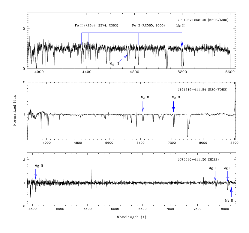
Figure 6: Representative normalized blazar spectra: J211552$+$000115 (top), J191816-411154 (middle), J073346+411120(bottom). In each case, the most redshifted Mg ii absorption system (thick blue arrow) detected was used as the lower limit to the blazar’s emission redshift. Thin blue lines in top panel mark the Fe ii ($\lambda$2344,2374,2383,2585,2600) lines associated with the Mg ii absorption line system at z${}_{\rm abs}=0.85840$.

References

- Anderson et al. (1987) Anderson S. F., Weymann R. J., Foltz C. B., Chaffee, Jr. F. H., 1987, AJ, 94, 278
- Antonucci (1993) Antonucci R., 1993, ARA&A, 31, 473
- Bahcall & Salpeter (1966) Bahcall J. N., Salpeter E. E., 1966, ApJ, 144, 847
- Bergeron et al. (2011) Bergeron J., Boissé P., Ménard B., 2011, A&A, 525, A51
- Chand & Gopal-Krishna (2012) Chand H., Gopal-Krishna, 2012, ApJ, 754, 38
- Chand et al. (2004) Chand H., Srianand R., Petitjean P., Aracil B., 2004, A&A, 417, 853
- Cucchiara et al. (2009) Cucchiara A., Jones T., Charlton J. C., Fox D. B., Einsig D., Narayanan A., 2009, ApJ, 697, 345
- Cucchiara et al. (2013) Cucchiara A. et al., 2013, ApJ, 773, 82
- Gehrels (1986) Gehrels N., 1986, ApJ, 303, 336
- Joshi et al. (2013) Joshi R., Chand H., Gopal-Krishna, 2013, MNRAS, 435, 346
- Khare et al. (1989) Khare P., York D. G., Green R., 1989, ApJ, 347, 627
- Komissarov (2017) Komissarov S., 2017, in IAU Symposium, Vol. 324, IAU Symposium, pp. 141–148
- Kulkarni et al. (2012) Kulkarni V. P., Meiring J., Som D., Péroux C., York D. G., Khare P., Lauroesch J. T., 2012, ApJ, 749, 176
- Massaro et al. (2009) Massaro E., Giommi P., Leto C., Marchegiani P., Maselli A., Perri M., Piranomonte S., Sclavi S., 2009, VizieR Online Data Catalog, 349
- Mathes et al. (2017) Mathes N. L., Churchill C. W., Murphy M. T., 2017, ArXiv e-prints
- Møller et al. (1994) Møller P., Jakobsen P., Perryman M. A. C., 1994, A&A, 287, 719
- Nestor et al. (2005) Nestor D. B., Turnshek D. A., Rao S. M., 2005, ApJ, 628, 637
- Padovani & Giommi (1995) Padovani P., Giommi P., 1995, MNRAS, 277, 1477
- Prochter et al. (2006) Prochter G. E. et al., 2006, ApJ, 648, L93
- Stocke & Rector (1997) Stocke J. T., Rector T. A., 1997, ApJ, 489, L17
- Sudilovsky et al. (2007) Sudilovsky V., Savaglio S., Vreeswijk P., Ledoux C., Smette A., Greiner J., 2007, ApJ, 669, 741
- Tejos et al. (2009) Tejos N., Lopez S., Prochaska J. X., Bloom J. S., Chen H.-W., Dessauges-Zavadsky M., Maureira M. J., 2009, ApJ, 706, 1309
- Tombesi et al. (2011) Tombesi F., Cappi M., Reeves J. N., Palumbo G. G. C., Braito V., Dadina M., 2011, ApJ, 742, 44
- Vergani et al. (2009) Vergani S. D., Petitjean P., Ledoux C., Vreeswijk P., Smette A., Meurs E. J. A., 2009, A&A, 503, 771
- Véron-Cetty & Véron (2010) Véron-Cetty M.-P., Véron P., 2010, A&A, 518, A10
- Wolfe et al. (2005) Wolfe A. M., Gawiser E., Prochaska J. X., 2005, ARA&A, 43, 861
- Zhu & Ménard (2013) Zhu G., Ménard B., 2013, ApJ, 770, 130