Corner effects on the perturbation of an electric potential

Abstract

We consider the perturbation of an electric potential due to an insulating inclusion with corners. This perturbation is known to admit a multipole expansion whose coefficients are linear combinations of generalized polarization tensors. We define new geometric factors of a simple planar domain in terms of a conformal mapping associated with the domain. The geometric factors share properties of the generalized polarization tensors and are the Fourier series coefficients of a generalized external angle of the inclusion boundary. Since the generalized external angle contains the Dirac delta singularity at corner points, we can determine a criteria for the existence of corner points on the inclusion boundary in terms of the geometric factors. We illustrate and validate our results with numerical examples computed to a high degree of precision using integral equation techniques, the Nyström discretization, and recursively compressed inverse preconditioning.

AMS subject classifications. 35R30; 30C35; 35J57

Key words. Generalized Polarization Tensors; Planar domain with corners; Riemann mapping; Schwarz-Christoffel Transformation; RCIP method

1 Introduction

Let $\Omega$ be a simply connected bounded domain in $\mathbb{R}^{2}$ containing the origin and with Lipschitz boundary. We suppose that the exterior of $\overline{\Omega}$ has unit conductivity and that $\Omega$ is insulated. Let $h$ be a harmonic function, and consider the following conductivity problem:

$$\begin{cases}\displaystyle\Delta u=0\quad&\mbox{in }\mathbb{R}^{2}\setminus\overline{\Omega},\\ \displaystyle\frac{\partial u}{\partial\nu}=0&\mbox{on }\partial\Omega,\\ \displaystyle u({\bf x})-h({\bf x})=O(|{\bf x}|^{-1})&\mbox{as }|{\bf x}|\to\infty.\end{cases}$$ (1.1)

The background potential $h$ here is perturbed by $u$ due to the presence of the inclusion $\Omega$. One can easily express the perturbation $u-h$ using a boundary integral equation formulation of (1.1) involving the Neumann-Poincaré (NP) operator. Furthermore, the boundary integral equation framework admits a multipole expansion of $u-h$ whose coefficients are linear combinations of the generalized polarization tensors (GPTs), which can also be expressed in terms of boundary integrals.

The GPTs are a sequence of real-valued tensors that are associated with $\Omega$ and they generalize the classical polarization tensors [28]. They can be obtained from multistatic measurements, where a high signal-to-noise ratio is needed to acquire high-order terms [2]. They have been used as building blocks when solving imaging problems for inclusions with smooth boundaries [4, 5]. The GPTs contain sufficient geometric information to determine $\Omega$ uniquely [5]. One can suitably approximate the conductivity, location, and shape of an inclusion, or several inclusions, using the first few leading terms of the GPTs by adopting an optimization framework [4, 9].

An inclusion with corners generally induces strong scattering close to corner points (vertices). The understanding and application of such corner effects is a subject of great interest. Detection methods for inclusions, from boundary measurements, have been developed in [22]. The gradient blow-up of the electrical potential for a bow-tie structure, which has two closely located domains with corners, was investigated in [25]. It has been shown that the spectral features of the NP operator of a domain with corners is significantly different from that of a smooth domain [11, 17, 19, 21, 27]. It is worth mentioning that the spectrum of the NP operator has recently drawn significant attention in relation to plasmonic resonances [1, 24, 32].

This paper analyzes the effects of inclusion corners on the perturbation of an electric potential. We present new geometric factors that clearly reveal the boundary information of an inclusion, including the existence of corner points. They satisfy mutually equivalent relations with the GPTs, so that one can compute them from the GPTs and vice versa. The geometric factors form an infinite sequence of complex numbers. The main result of this paper is that the geometric factors are actually the Fourier series coefficients of a generalized external angle function (for a precise statement, see Theorem 4.2). The generalized external angle function has the Dirac delta singularity at corner points. As a consequence, we can determine when there exist corner points: the geometric factor sequence converges to zero when the inclusion has a smooth boundary. However, it does not converge to zero, but oscillates, if there is any corner point on the boundary of the inclusion. In practice, only a finite number of leading terms of the GPTs can be obtained due to the limitation of the signal-to-noise ratio in the measurements. If sufficiently many terms of the GPTs are given, then the partial Fourier series sum of the generalized external angle function computed with the GPTs shows isolated high peaks at corner points, as illustrated in Section 5.

Our derivation is motivated by the recent result [23], where explicit relationships between the exterior Riemann mapping coefficients and the GPTs were derived. In addition, we consider the internal conformal mapping, with which the geometric factors are defined and which is obtained by reflecting the exterior Riemann mapping function across the unit circle. We prove the Fourier relation between the geometric factors and the generalized external angle by applying the Carathéodory mapping theorem on the uniform convergence of conformal mappings (see Appendix A).

One can numerically compute the GPTs for an arbitrary domain with corners to a high degree of precision using integral equation techniques, the Nyström discretization, and recursively compressed inverse preconditioning (RCIP) [20]. The geometric factors can then be obtained from their relations with the GPTs. We present some numerical examples to validate and visualize our results.

The rest of the paper is organized as follows: In Section 2 we derive explicit connections between the GPTs and the coefficients of the Riemann mappings and define the geometric factors. In Section 3 we express the geometric factors for curvilinear polygons in terms of vertices and external angles. Section 4 is about equivalent relations between the geometric factors and the GPTs for arbitrary Lipschitz domains and the investigation of corner effects. Section 5 presents numerical examples. We prove several recursive relations in Section 6, and we conclude with some discussion.

2 Generalized polarization tensors and Riemann mappings

2.1 Multipole Expansion

We identify ${\bf x}=(x_{1},x_{2})$ in $\mathbb{R}^{2}$ with $z=x_{1}+{\rm{i}}x_{2}\in\mathbb{C}$ for notational convenience. Let $h({\bf x})=\mbox{Re}\{H(z)\}$ with

$$H(z)=\alpha_{0}+\sum_{n=1}^{\infty}\alpha_{n}z^{n},\quad\alpha_{n}=a_{n}^{c}+{\rm i}a_{n}^{s}.$$

Then, it is shown in [6, 7] that the solution $u$ to (1.1) satisfies $u({\bf x})=\mbox{Re}\{U(z)\}$, where $U$ is a complex analytic function in $\mathbb{C}\setminus\overline{\Omega}$ such that

$$U(z)=\alpha_{0}+\sum_{n=1}^{\infty}\left[a_{n}^{c}\left(z^{n}-\sum_{m=1}^{\infty}\frac{\gamma_{mn}^{1}+\gamma_{mn}^{2}}{z^{m}}\right)+{\rm i}a_{n}^{s}\left(z^{n}-\sum_{m=1}^{\infty}\frac{\gamma_{mn}^{1}-\gamma_{mn}^{2}}{z^{m}}\right)\right]$$ (2.1)

for $|z|$ sufficiently large with

$$\begin{cases}\displaystyle\gamma_{kn}^{1}=\frac{1}{4\pi k}\left[M_{kn}^{cc}-M_{kn}^{ss}+{{\rm{i}}}(M_{kn}^{cs}+M_{kn}^{sc})\right],\\[5.69054pt] \displaystyle\gamma_{kn}^{2}=\frac{1}{4\pi k}\left[M_{kn}^{cc}+M_{kn}^{ss}-{{\rm{i}}}(M_{kn}^{cs}-M_{kn}^{sc})\right],\quad k,n\in\mathbb{N}.\end{cases}$$ (2.2)

Here the quantities $\{M_{kn}^{\alpha\beta}\}_{k,n\in\mathbb{N}}$ ($\alpha,\beta\in\{c,s\}$) are the so-called (contracted) GPTs. The zero Neumann condition on $\partial\Omega$ in (1.1) implies that

$$\Im U\,=\,\mbox{constant on }\partial\Omega.$$ (2.3)

The GPTs are defined in terms of boundary integrals as follows: We set polar coordinates

$$P_{n}^{c}({\bf x})=r^{n}\cos n\theta\,,\qquad P_{n}^{s}({\bf x})=r^{n}\sin n\theta\,,$$

and define

$$M^{\alpha\beta}_{kn}:=\int_{\partial\Omega}P_{k}^{\beta}({\bf x})(-\frac{1}{2}I-\mathcal{K}^{*}_{\partial\Omega})^{-1}[\nu\cdot\nabla P_{n}^{\alpha}]({\bf x})\,d\sigma({\bf x})$$ (2.4)

for $k,n\in\mathbb{N}$ and $\alpha,\beta\in\{c,s\}$. The operator $\mathcal{K}^{*}_{\partial\Omega}$ is the Neumann-Poincaré (NP) operator

$$\mathcal{K}^{*}_{\partial\Omega}[\varphi]({\bf x})=\frac{1}{2\pi}p.v.\int_{\partial\Omega}\frac{\langle{\bf x}-{\bf y},\nu_{\bf x}\rangle}{|{\bf x}-{\bf y}|^{2}}\varphi({\bf y})\,d\sigma({\bf y})\;,\quad{\bf x}\in\partial\Omega,$$ (2.5)

where $\nu_{\bf x}$ is the outward unit normal vector to $\partial\Omega$ and $p.v.$ denotes the Cauchy principal value. It was shown in [15, 30] that $\lambda I-\mathcal{K}_{\partial\Omega}^{*}$ is invertible on $L^{2}_{0}(\partial\Omega)$ for $|\lambda|\geq 1/2$. See [6] for more properties of the NP operator.

From (2.2), one can get the $M_{kn}^{\alpha\beta}$ from the $\gamma_{kn}^{j}$ and vice versa. In this sense we will refer to the $\gamma_{kn}^{j}$ as GPTs as well in this paper. It is worth mentioning that the contracted GPTs have been used in making a near-cloaking structure [7, 8] and that they can be used as shape descriptors [4]. More applications of the GPTs can be found in [3] and references therein.

2.2 Two Riemann mapping functions

Since $\Omega$ is simply connected, thanks to the Riemann mapping theorem there exists a unique exterior Riemann mapping $\Phi:\mathbb{C}\setminus\mathbb{D}\to\mathbb{C}\setminus\Omega$ of the form

$$\Phi[\Omega](\zeta)=C\left(\mu_{-1}\zeta+\mu_{0}+\frac{\mu_{1}}{\zeta}+\frac{\mu_{2}}{\zeta^{2}}+\cdots\right),$$ (2.6)

where $\mathbb{D}$ denotes the unit disc centered at the origin, $C>0$ is a constant, and we set $\mu_{-1}=1$. We may simply write $\Phi(\zeta)$ when the domain is clear from the context. For $k\geq 1$, the coefficients $\mu_{k}$ are invariant under translation and scaling of $\Omega$. In [23], an explicit relation was derived between the exterior Riemann mapping coefficients $\mu_{k}$ and the GPTs associated with $\Omega$. This means that one can compute the $\mu_{k}$ from the GPTs.

In this paper, we additionally consider the internal conformal mapping $S$ that is obtained by reflecting the exterior Riemann mapping function across the unit circle. Remind that we assume $0\in\Omega$. We will then derive formulas for the GPTs using both the coefficients of $\Phi$ and those of $S$.

By ${\Omega^{r}}$ we denote the reflection of $\Omega$ across the unit circle, i.e.,

$${\Omega^{r}}:=\Bigr{\{}\frac{1}{\zeta}\;|\;\zeta\in\mathbb{C}\setminus\overline{\Omega}\Bigr{\}}\cup\{0\}.$$ (2.7)

Note that $(\Omega^{r})^{r}=\Omega$. We also define $S[\Omega^{r}]:\mathbb{D}\rightarrow\Omega^{r}$ by

$$S[\Omega^{r}](w):=\begin{cases}\displaystyle\frac{1}{\Phi[\Omega](\frac{1}{w})}\quad&\mbox{for }w\in\mathbb{D}\setminus\{0\},\\ \displaystyle 0\quad&\mbox{for }w=0.\end{cases}$$ (2.8)

We may simply write $S(w)$ when the domain is clear from the context. Then, ${\Omega^{r}}$ is a simply connected domain containing $0$ and $S:\mathbb{D}\rightarrow{\Omega^{r}}$ is the interior Riemann mapping corresponding to $\Omega^{r}$ satisfying $S(0)=0$ and $S^{\prime}(0)>0$. It is obvious from (2.6) that $S$ admits the series expansion

$$S[\Omega^{r}](w)=\frac{1}{C}\left(b_{1}w+b_{2}w^{2}+\cdots\right)\quad\mbox{in }\mathbb{D}$$ (2.9)

with some complex numbers $b_{k}$. Note that $b_{1}=1$ because $\mu_{-1}=1$.

Lemma 2.1.

The coefficients of $\Phi[\Omega]$ have the following equivalent relation with those of $S[\Omega^{r}]$:

$$\mu_{k-1}+b_{k+1}+\sum_{j=2}^{k}b_{j}\mu_{k-j}=0\,,\quad k\geq 1\,.$$ (2.10)

Proof.  For $0<|w|<1$, we have

$$1 =S[\Omega^{r}](w)\cdot\Phi[\Omega](1/w)=\left(\sum_{j=1}^{\infty}b_{j}w^{j}\right)\left(\sum_{j=-1}^{\infty}\mu_{k}w^{k}\right)=1+\sum_{k=1}^{\infty}\left(\sum_{j=1}^{k+1}b_{j}\mu_{k-j}\right)w^{k}$$

Since $b_{1}=\mu_{-1}=1$, this proves the lemma.∎

2.3 Generalized polarization tensors and Riemann mappings coefficients

Let $V_{1}$ be the analytic function in $\mathbb{C}\setminus\overline{\Omega}$ such that $\Re\{V_{1}(z)\}$ be the solution to (1.1) with $h(\mathbf{x})=\Re\{z^{n}\}$. Similarly, we define $V_{2}$ the analytic function in $\mathbb{C}\setminus\overline{\Omega}$ such that $\Re\{{\rm i}V_{2}(z)\}$ be the solution with $h(\mathbf{x})=\Re\{{\rm i}z^{n}\}$. From (2.1) we have

$$\left(V_{1}\circ\Phi\right)(\zeta)=\Phi(\zeta)^{n}-\sum_{m=1}^{\infty}\frac{\gamma_{mn}^{1}+\gamma_{mn}^{2}}{\Phi(\zeta)^{m}},$$

$$\left(V_{2}\circ\Phi\right)(\zeta)=\Phi(\zeta)^{n}-\sum_{m=1}^{\infty}\frac{\gamma_{mn}^{1}-\gamma_{mn}^{2}}{\Phi(\zeta)^{m}}$$

for sufficiently large $|\zeta|$. As discussed in (2.3) the zero Neumann condition in (1.1) implies $\Im\{V_{1}\circ\Phi(\zeta)\},\,\Im\{{\rm i}V_{2}\circ\Phi(\zeta)\}$ are constants for $|\zeta|=1$ and, thus,

$$\rm{i}\Im\{V_{1}\circ\Phi\}+\Im\{{\rm i}V_{2}\circ\Phi\}\,=\,\mbox{constant for }|\zeta|=1.$$ (2.11)

Note that

$$\rm{i}\Im\{V_{1}\circ\Phi\}+\Im\{{\rm i}V_{2}\circ\Phi\} =\frac{1}{2}\left(V_{1}\circ\Phi+V_{2}\circ\Phi\right)(\zeta)-\frac{1}{2}\overline{\left(V_{1}\circ\Phi-V_{2}\circ\Phi\right)(\zeta)}$$

$$=\Phi(\zeta)^{n}-\sum_{m=1}^{\infty}\frac{\gamma_{mn}^{1}}{\Phi(\zeta)^{m}}+\overline{\sum_{m=1}^{\infty}\frac{\gamma_{mn}^{2}}{\Phi(\zeta)^{m}}},$$ (2.12)

where the second equality holds for sufficiently large $|\zeta|$. This induces the following lemma, which plays an essential role in deriving relations between the GPTs and the $\mu_{k}$ in [23].

Lemma 2.1.

([23]) The function $V_{1}\circ\Phi+V_{2}\circ\Phi$ has an entire extension.

To state our result, we define two multi-index sequences $\{\mu_{n,k}\}$ and $\{b_{n,k}\}$ ($n,k\in\mathbb{N}$, $k\geq n$) such that the following formal expansions hold:

$$\sum_{k=n}^{\infty}\mu_{n,k}{x^{k}}=\left(\sum_{k=1}^{\infty}\mu_{k-2}x^{k}\right)^{n},\quad\sum_{k=n}^{\infty}{b_{n,k}}{x^{k}}=\left(\sum_{k=1}^{\infty}b_{k}x^{k}\right)^{n}.$$

In other words

$$\mu_{n,k} =\sum_{s_{1}+s_{2}+\cdots+s_{k}=n,\atop s_{1}+2s_{2}+\cdots+ks_{k}=k}\frac{n!}{s_{1}!s_{2}!\cdots s_{k}!}{\mu_{-1}}^{s_{1}}{\mu_{0}}^{s_{2}}\cdots{\mu_{k-2}}^{s_{k}},$$

$$b_{n,k} =\sum_{s_{1}+s_{2}+\cdots+s_{k}=n,\atop s_{1}+2s_{2}+\cdots+ks_{k}=k}\frac{n!}{s_{1}!s_{2}!\cdots s_{k}!}{b_{1}}^{s_{1}}{b_{2}}^{s_{2}}\cdots{b_{k}}^{s_{k}}.$$

Here, $s_{1},\ldots,s_{k}$ are non-negative integers. In particular, we have

$$b_{1,k}=b_{k}\,,\quad\mu_{1,k}=\mu_{k-2}\,,\quad\mu_{k,k}=\mu_{-1}^{k}=1\,,\quad b_{k,k}=b_{1}^{k}=1\,.$$ (2.13)

We can deduce the following proposition using $\mu_{n,k}$ and $b_{n,k}$. See Section 6.1 for a detailed proof. Lemma 2.1 plays an essential role in the derivation.

Proposition 2.2.

The GPTs associated with $\Omega$ have recurrence formulas with the coefficients of $\Phi[\Omega]$ and $S[\Omega^{r}]$. For each $k,n\in\mathbb{N}$, we have

$$\displaystyle\gamma_{kn}^{1} =C^{k+n}\left(\mu_{n,2n+k}-\sum_{m=1}^{k-1}\frac{\gamma_{mn}^{1}}{C^{m+n}}b_{m,k}\right),$$ (2.14)

$$\displaystyle\gamma_{kn}^{2} =\begin{cases}\displaystyle-C^{k+n}\left(\bar{\mu}_{n,2n-k}+\sum_{m=1}^{k-1}\frac{\gamma_{mn}^{2}}{C^{m+n}}b_{m,k}\right),\qquad&k\leq n\,,\\[4.2679pt] \displaystyle-C^{k+n}\sum_{m=1}^{k-1}\frac{\gamma_{mn}^{2}}{C^{m+n}}b_{m,k}\,,\qquad&k\geq n+1\,.\end{cases}$$ (2.15)

We can also express $b_{k}$ and $\mu_{k}$ by the GPTs as follows. See Section 6.2 for a proof.

Proposition 2.3.

We have

$$C =\sqrt{-\gamma_{11}^{2}}\,,$$ (2.16)

$$b_{k} =\sum_{m=2}^{k}\frac{\gamma_{m1}^{2}}{C^{m+1}}b_{m,k}\,,\quad k\geq 2\,.$$ (2.17)

For example, with $k=2,3$ in (2.17) we deduce, using $b_{2,3}=2b_{2}$, that

$$b_{2}=\gamma_{21}^{2}\left(-\gamma_{11}^{2}\right)^{-\frac{3}{2}},\quad b_{3}=2(\gamma_{21}^{2})^{2}\left(-\gamma_{11}^{2}\right)^{-3}+{\gamma_{31}^{2}}\left(-\gamma_{11}^{2}\right)^{-2}\,.$$

Now, with $k=1,2$ in (2.10) we have $\mu_{0}=-b_{2}$ and $\mu_{1}=-b_{3}-b_{2}\mu_{0}$.

Remark 1.

We can show, as proved in Section 6.2, that $b_{k}$ also satisfies

$$\gamma_{11}^{1}b_{k}={C^{2}}\left(\mu_{k}-\sum_{m=2}^{k}\frac{\gamma_{m1}^{1}}{C^{m+1}}b_{m,k}\right),\quad k\geq 2\,.$$ (2.18)

Through this relation as well as (2.17), we can see that there are domain-independent relationships among the GPTs. Additional examples are provided in [23].

2.4 Geometric factor $\sigma_{k}$ and equivalent relations

Definition 1.

We define a new sequence of geometric factors $\{\sigma_{k}\}_{k=1}^{\infty}$ for $\Omega$ as

$$\sigma_{k}[\Omega]:=k(k+1)b_{k+1}-\sum_{j=1}^{k-1}(j+1)b_{j+1}{\sigma_{k-j}}\,,\qquad k\geq 1\,.$$ (2.19)

We can simplify this definition as $\displaystyle\{\sigma_{k}\}_{k=1}^{\infty}=\mathcal{P}\big{(}\{b_{k}\}_{k=2}^{\infty}\big{)}$ or

$$\sigma_{k}=\sum_{i_{1}+2i_{2}+\cdots+ki_{k}=k}P_{k,i_{1},\ldots,i_{k}}b_{2}^{i_{1}}\cdots b_{k+1}^{i_{k}}\,,$$ (2.20)

with some integer coefficients $P_{k,i_{1},\ldots,i_{k}}$. Here, $i_{1},\ldots,i_{k}$ are non-negative integers.

The definition (2.19) implies that $\mathcal{P}$ is invertible. Thanks to the relations between the GPTs and the Riemann mapping coefficients in the previous section, we can see that there are mutually equivalent connections among the GPTs $\gamma_{kn}^{j}$, the exterior Riemann mapping coefficients $\mu_{k}$, the interior Riemann mapping coefficients $b_{k}$, and the geometric factors $\sigma_{k}$. For instance, we have

$$b_{2}=\frac{1}{2}\sigma_{1},\quad b_{3}=\frac{1}{6}\left(\sigma_{2}+\sigma_{1}^{2}\right),\quad b_{4}=\frac{1}{24}\left(2\sigma_{3}+3\sigma_{1}\sigma_{2}+\sigma_{1}^{3}\right)$$

$$\mu_{0}=-\frac{1}{2}\sigma_{1}\,,\quad \mu_{1}=\frac{1}{12}\left(-2\sigma_{2}+\sigma_{1}^{2}\right)\,,\quad \mu_{2}=\frac{1}{24}\left(-2\sigma_{3}+\sigma_{1}\sigma_{2}\right)\,,$$

and

$$\gamma^{1}_{11}=-\frac{C^{2}}{6}\sigma_{2}+\frac{C^{2}}{12}\sigma_{1}^{2},\quad\gamma_{12}^{1}=-\frac{C^{3}}{6}\sigma_{3}+\frac{C^{3}}{4}\sigma_{1}\sigma_{2}-\frac{C^{3}}{12}\sigma_{1}^{3},\quad\gamma_{21}^{1}=-\frac{C^{3}}{12}\sigma_{3}+\frac{C^{3}}{8}\sigma_{1}\sigma_{2}-\frac{C^{3}}{24}\sigma_{1}^{3}\,,$$

$$\gamma_{11}^{2}=-C\bar{C}\,,\qquad\gamma_{12}^{2}=C\bar{C}^{2}\sigma_{1}\,,\qquad\gamma_{21}^{2}=\frac{C^{2}\bar{C}}{2}\sigma_{1}\,.$$

3 Geometric factor for a curvilinear polygon

In this section we restrict $\Omega$ to be a curvilinear polygon, in other words $\Omega=P^{r}$ with a simple polygon $P$, and deduce explicit connections between the geometric factors and the corner geometry of $\Omega$. Figure 5.1(a,b) illustrate a curvilinear polygon and its reflection across the unit circle. More specifically, we let $P$ be a simply connected region bounded by a polygon whose vertices are $A_{1},\ldots,A_{n}$ (ordered consecutively) with $n\geq 3$ and with external angles $\beta_{1}\pi,\ldots,\beta_{n}\pi$. We assume $0\in P$. Note that $-1<\beta_{j}<1$ and $\sum_{j=1}^{n}\beta_{j}=2$.

It is well known that the interior conformal mapping of a simple polygon can be expressed as the Schwarz-Christoffel integral. For the polygon $P$ described above, we have

$$S[P](z)=C_{1}\int_{0}^{z}{\prod_{j=1}^{n}\left(w-a_{j}\right)^{-\beta_{j}}}dw+C_{2}\,,$$

where $C_{1}$ and $C_{2}$ are complex constants, and $a_{1},\ldots,a_{n}$ are $n$ distinct pre-vertices on $\partial\mathbb{D}$ satisfying $S(a_{j})=A_{j}$ for each $j=1,\ldots,n$. One can find a detailed explanation of the Schwarz-Christoffel integral in many textbooks, for example in [29].

Assuming $S(0)=0$ and $S^{\prime}(0)=1/C>0$, we have a slightly different formulation:

$$S[P](z)=\frac{1}{C}\int_{0}^{z}\pi(w)\,dw\,,\qquad\pi(z)={\prod_{j=1}^{n}\left(1-\frac{z}{a_{j}}\right)^{-\beta_{j}}}\,.$$ (3.1)

Here, the branch-cut is given such that $\pi(0)=1$. The coefficients in the expansion (2.9) satisfy $C\cdot S^{\prime}(z)=1+\sum_{k=1}^{\infty}b_{k+1}(k+1)z^{k}$. From the fact $\pi(z)=C\cdot S^{\prime}(z)$ we deduce

$$b_{k+1}=\frac{\pi^{(k)}(0)}{(k+1)!}\,.$$ (3.2)

Lemma 3.1.

For the polygon $P$ described above, we have for each $k\in\mathbb{N}$

$$\sigma_{k}[P^{r}]=\sum_{j=1}^{n}\beta_{j}a_{j}^{-k}.$$ (3.3)

Proof.  Set $\widetilde{\sigma}_{k}=\sum_{j=1}^{n}\beta_{j}a_{j}^{-k}$ and consider the function

$$F_{k}(w)=(k-1)!\sum_{j=1}^{n}\beta_{j}{a_{j}}^{-k}\left(1-\frac{w}{a_{j}}\right)^{-k},\quad k\geq 1\,.$$

One can easily see that $\pi^{\prime}=\pi F_{1}$ and ${F_{k}}^{\prime}=F_{k+1}$. Applying the Leibniz rule, we have

$$\pi^{(k)}=(\pi F_{1})^{(k-1)}=\sum_{j=0}^{k-1}{k-1\choose j}{\pi}^{(j)}{F_{1}}^{(k-1-j)}=\sum_{j=0}^{k-1}{k-1\choose j}{\pi}^{(j)}{F_{k-j}}.$$

Note that $F_{k}(0)=(k-1)!\,\widetilde{\sigma}_{k}$. Evaluating the above equation at $0$, we prove

$$\pi^{(k)}(0)=(k-1)!\,\widetilde{\sigma}_{k}+\sum_{j=1}^{k-1}\frac{(k-1)!}{j!}\pi^{(j)}(0){\widetilde{\sigma}_{k-j}}.$$ (3.4)

The lemma then follows as a direct consequence of (3.2) and (2.19).∎

4 Analysis of corner effects

We now consider an arbitrary planar domain with corners. We assume that $\Omega$ is a simply connected domain bounded by a piecewise regular analytic curve with a finite number of corners. Figures 5.2(a,b) illustrate an example of such domain and its reflection across the unit circle.

We characterize the corner effects in the geometric factor (and as a result, in the GPTs or in Riemann mapping coefficients) by approximating $\Omega^{r}$ with simple polygons.

4.1 Generalized external angle of $\partial{\Omega^{r}}$

Let $S[\Omega^{r}]:\mathbb{D}\rightarrow\Omega^{r}$ be given as in Section 2.2. Since $\partial\Omega$ is a piecewise regular analytic curve, so is $\partial{\Omega^{r}}$. Since $\partial{\Omega^{r}}$ is a Jordan curve, the interior Riemann mapping $S$ extends to a bijective continuous function from $\overline{\mathbb{D}}$ to $\overline{{\Omega^{r}}}$. Let $\zeta$ be an arbitrary point on $\partial\Omega^{r}$ which is not a corner point. Then the inverse mapping $S^{-1}:\Omega^{r}\rightarrow\mathbb{D}$ extends holomorphically across $\zeta$ (see [12]) and $(S^{-1})^{\prime}(\zeta)\neq 0$ (see [13, Theorem 18, p. 217, and Theorem 20, p. 226]). From the inverse function theorem, $S$ is smooth near $S^{-1}(\zeta)$. We assume that the curvature of $\partial\Omega^{r}$ is uniformly bounded except at the corner points.

Denote $\alpha(t)=(x(t),y(t))$, $t\in[0,1]$, the piecewise analytic parametrization of $\partial\Omega^{r}$ by the Riemann mapping $S[\Omega^{r}]$. In other words

$$\alpha(t)=S[\Omega^{r}](e^{2\pi t{\rm i}})\,,\qquad t\in[0,1]\,,$$

together with finitely many points $0\leq t_{1}<\cdots<t_{M}<1$, where $\alpha(t_{l})$, $l=1,\ldots,M$, are corner points on $\partial\Omega^{r}$. We set $t_{M+1}=t_{1}+1$ and regard $\alpha$ as a periodic function with period $1$, for notational convenience. Owing to the assumption $C>0$ in series expansions for $S$, $\alpha$ has positive orientation. We define the external angle $\beta_{l}\pi$ at each corner $\alpha(t_{l})$ by the signed angle between the two vectors $\alpha^{\prime}(t_{l}-)$ and $\alpha^{\prime}(t_{l}+)$, i.e., $\beta_{l}\in(-1,1)$ and

$$\beta_{l}\pi=\arg\left(\alpha^{\prime}(t_{l}+)\right)-\arg\left(\alpha^{\prime}(t_{l}-)\right)$$ (4.1)

with a modulus of $2\pi$. We then generalize the concept of external angle for any boundary points as follows. The generalized external angle is essential in understanding corner effects in perturbations of an electric potential.

Definition 1.

Define a function $\Theta:[0,1]\to\mathbb{R}$ as

$$\Theta(t):=\frac{1}{\pi}k_{\rm{g}}(t)|\alpha^{\prime}(t)|+\sum_{l=1}^{M}\beta_{l}\delta(t-t_{l})\,,\quad t\in[0,1]\,,$$ (4.2)

where $k_{\rm{g}}$ denotes the (geodesic) curvature of $\alpha$ in $\mathbb{R}^{2}$, i.e.,

$$k_{\rm{g}}(t)=\frac{x^{\prime}(t)y^{\prime\prime}(t)-x^{\prime\prime}(t)y^{\prime}(t)}{|\alpha^{\prime}(t)|^{3}}\,.$$

We call $\pi\Theta(t)$ the generalized external angle of $\partial{\Omega^{r}}$ at $\alpha(t)$. We may indicate the associated domain by writing $\Theta[\partial{\Omega^{r}}]$ if necessary.

Recall that the internal angle is $\pi(1-\beta)$ at the corner $\alpha(t_{l})$. From [31] we have $S^{-1}(z)\sim(z-\alpha(t_{l}))^{\frac{1}{1-\beta}}$ for $z\in\Omega^{r}$ near $\alpha(t_{l})$ and, thus, $\alpha(t)\sim(t-t_{l})^{1-\beta}$. Here, $f\sim g$ near $z_{0}$ means $\lim_{z\rightarrow z_{0}}\frac{f(z)}{g(z)}\in\mathbb{C}\setminus\{0\}$. Therefore, $\frac{1}{\pi}k_{\rm{g}}(t)|\alpha^{\prime}(t)|$ is integrable. From the Gauss-Bonnet formula we have

$$\int_{0}^{1}\Big{[}k_{\rm{g}}(t)|\alpha^{\prime}(t)|+\sum_{l=1}^{N}\beta_{l}\pi\delta(t-t_{l})\Big{]}dt=\int_{\partial\Omega}k_{\rm{g}}(s)ds+\sum_{l=1}^{N}\beta_{l}\pi=2\pi\,.$$ (4.3)

4.2 Approximation of ${\Omega^{r}}$ by a sequence of polygons

Fix $n\in\mathbb{N}$ and consider equally distanced nodes $\big{\{}\frac{j}{n}|1\leq j\leq n\big{\}}$ on $[0,1]$. For each $l=1,\ldots,M$, let $j_{l}$ be the index such that $\alpha(\frac{j_{l}}{n})$ is the nearest point in $\big{\{}\alpha(\frac{j}{n})|1\leq j\leq n\big{\}}$ to the corner point $\alpha(t_{l})$. We set

$$p_{n,j} =\displaystyle\begin{cases}\alpha(t_{l}),\quad&\mbox{if }j=j_{l}\mbox{ for some }l=1,\ldots,M,\\ \alpha(\frac{j}{n}),\quad&\mbox{otherwise},\end{cases}$$

$$e_{n,j} =\displaystyle\begin{cases}e^{2\pi t_{l}{\rm i}},\quad&\mbox{if }j=j_{l}\mbox{ for some }l=1,\ldots,M,\\ e^{2\pi\frac{j}{n}{\rm i}},\quad&\mbox{otherwise}.\end{cases}$$

We denote by $P_{n}$ the polygon defined by the chain of edges $[p_{n,j},p_{n,j+1}]$, $j=1,\ldots,n$, with $p_{n,n+1}=p_{n,1}$. We let $\beta_{n,j}\pi$ be the external angle of $P_{n}$ at each $p_{n,j}$. Recall that $\beta_{n,j}\in(-1,1)$.

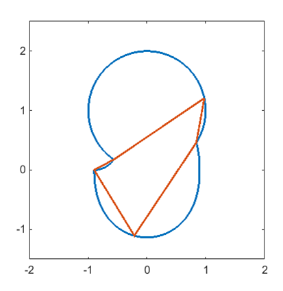
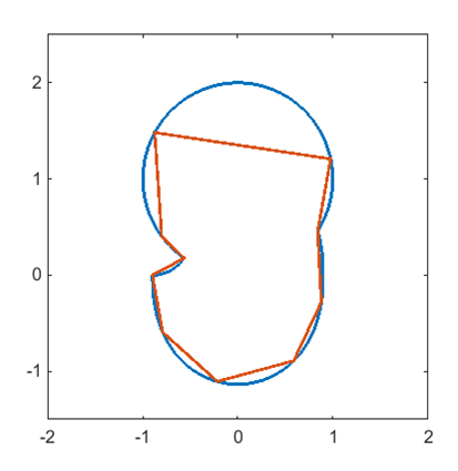
Figure 4.1: The polygon $P_{n}$ (in red) approximates ${\Omega^{r}}$ (in blue), where $\Omega$ is given as in Figure 5.2. The number of edges are $n=5,10,40$ from the left to the right.

The polygon $P_{n}$ is an $n$-sided simple polygon with sufficiently large $n$, and one can show that the sequence of polygons $P_{n}$ converges in the sense of Carathéodory to its kernel $\Omega^{r}$. See Appendix A for the definition of such convergence. Figure 4.1 shows how $P_{n}$ approximates to $\Omega^{r}$ as $n$ increases. We can obtain the asymptotic for the external angles.

Lemma 4.1.

Let $n$ be large enough so that $P_{n}$ is a simple polygon. For $p_{n,j}$ located away from corner points, we have

$$\beta_{n,j}=\displaystyle\frac{1}{n\pi}{k_{\rm{g}}\left(\frac{j}{n}\right)}\left|\alpha^{\prime}\left(\frac{j}{n}\right)\right|+o(\frac{1}{n}).$$ (4.4)

Proof.  We set $h=\frac{1}{n}$ and $t=\frac{j}{n}$. Note that the external angle $\beta_{n,j}\pi$ is the relative angle of $\alpha(t+h)-\alpha(t)$ with respect to the direction of $\overrightarrow{\alpha(t-h)\alpha(t)}$. Let us denote

$$\Delta^{\pm}_{h}\alpha(t)=\pm\left(\alpha(t\pm h)-\alpha(t)\right).$$

Then the angle $\beta_{n,j}$ satisfies

$$\left|\beta_{n,j}\right|=\frac{1}{\pi}\arccos\left(\frac{\langle\Delta^{+}_{h}\alpha(t),\ \Delta^{-}_{h}\alpha(t)\rangle}{|\Delta^{+}_{h}\alpha(t)|\cdot|\Delta^{-}_{h}\alpha(t)|}\right).$$

Let us suppose that $p_{n,j}=\alpha(\frac{j}{n})$ is located away from corner points. By applying the Taylor’s Theorem, we have

$$\Delta^{\pm}_{h}\alpha(t)=\alpha^{\prime}(t)h\pm\frac{\alpha^{\prime\prime}(t)}{2!}h^{2}+\frac{\alpha^{\prime\prime\prime}(t)}{3!}h^{3}+o(h^{3})$$

and, therefore,

$$\frac{\langle\Delta^{+}_{h}\alpha(t),\ \Delta^{-}_{h}\alpha(t)\rangle}{|\Delta^{+}_{h}\alpha(t)|\cdot|\Delta^{-}_{h}\alpha(t)|} =1-\frac{h^{2}}{2}\left(\frac{x^{\prime}(t)y^{\prime\prime}(t)-x^{\prime\prime}(t)y^{\prime}(t)}{[x^{\prime}(t)]^{2}+[y^{\prime}(t)]^{2}}\right)^{2}+o(h^{2})$$

$$=1-\frac{h^{2}}{2}k_{\rm{g}}(t)^{2}|\alpha^{\prime}(t)|^{2}+o(h^{2}).$$

Therefore, we get

$$\left|\beta_{n,j}\right|=\frac{h}{\pi}|k_{\rm{g}}(t)||\alpha^{\prime}(t)|+o(h)=\displaystyle\frac{1}{n\pi}{\left|k_{\rm{g}}\left(\frac{j}{n}\right)\right|}\left|\alpha^{\prime}\left(\frac{j}{n}\right)\right|+o\left(\frac{1}{n}\right).$$

Since the magnitude of $\beta_{n,j}$ is small due to $t$ not being a corner point, the sign of $\beta_{n,j}$ coincides with that of the cross product $(\nabla_{h}^{-}\alpha(t))\times(\nabla_{h}^{+}\alpha(t))$. Since $(\nabla_{h}^{-}\alpha(t))\times(\nabla_{h}^{+}\alpha(t))$ has the same sign as $k_{\rm{g}}(\frac{j}{n})$, we prove the lemma. ∎

Since $\partial\Omega^{r}$ is a piecewise analytic curve, we have from a similar analysis as in the previous lemma that for any $\epsilon>0$, there exists $\delta=\delta(\epsilon)>0$ such that

$$\sum_{p_{n,j}\in B_{\delta}}|\beta_{n,j}|<\epsilon$$ (4.5)

with $B_{\delta}=\cup_{l=1}^{M}\left\{z\in\partial P_{n}:0<|z-\alpha(t_{l})|<\delta\right\}$. Since $\alpha(t)\sim(t-t_{l})^{1-\beta}$, we have

$$\left|\frac{j}{n}-t_{l}\right|=O(\delta^{\frac{1}{1-\beta}})\quad\mbox{for }p_{n,j}\in B_{\delta}.$$ (4.6)

Riemann mapping functions. We set $\Omega_{n}=(P_{n})^{r}$ and, thus, $(\Omega_{n})^{r}=P_{n}$. The Riemann mapping functions $\Phi[\Omega_{n}]$ and $S[P_{n}]$ admit the series expansions

$$\Phi[\Omega_{n}](z) =C_{n}\left(\mu_{n,-1}z+\mu_{n,0}+\frac{\mu_{n,1}}{z}+\frac{\mu_{n,2}}{z^{2}}+\cdots\right),\quad z\in\mathbb{C}\setminus\mathbb{D}\,,$$

$$S[P_{n}](z) =\frac{1}{C_{n}}\left(b_{n,1}z+b_{n,2}z^{2}+b_{n,3}z^{3}+\cdots\right),\quad z\in\mathbb{D}\,,$$

with $\mu_{n,-1}=b_{n,1}=1$ and some constants $C_{n}>0$.

Since $P_{n}$ converges in the sense of Carathéodory to its kernel ${\Omega^{r}}$, we have uniform convergence from $S[P_{n}]$ to $S[\Omega^{r}]$ and from $\Phi[\Omega_{n}]$ to $\Phi[\Omega]$ as $n\rightarrow\infty$ from the Carathéodory’s mapping theorem (see Appendix A for the statement and references). Therefore, for each $k$ we have

$$\mu_{n,k}\rightarrow\mu_{k}\,,\quad b_{n,k}\rightarrow b_{k}\,,\quad C_{n}\rightarrow C\,,\quad\mbox{as }n\rightarrow\infty\,.$$

Here, $\mu_{k},\,b_{k},\,C$ are coefficients corresponding to $\Omega$. From (2.20) we have for each $k$

$$\sigma_{k}[\Omega_{n}]\rightarrow\sigma_{k}[\Omega]\,,\quad\mbox{as }n\rightarrow\infty\,.$$ (4.7)

Since the boundary of $\Omega^{r}$ is a Jordan curve, the corresponding Riemann mapping $S[\Omega^{r}]$ extends to a bijective continuous function from $\overline{\mathbb{D}}$ onto $\overline{\Omega^{r}}$ as explained before. From the Carathéodory’s mapping theorem, $S[P_{n}]^{-1}$ converges uniformly to $S[\Omega]^{-1}$ on any compact subset of $\Omega$ as $n\to\infty$. Moreover, it was proved in [26, pp. 75–79, vol. 2] that $S[P_{n}]^{-1}$ converges uniformly to $S[\Omega]^{-1}$ on $\overline{\Omega^{r}}$ if $P_{n}$ decreases to $\Omega^{r}$. In the proof, the equicontinuity of $\{S[P_{n}]^{-1}\}$ plays an essential role. By slightly modifying the proof of [26, Theorem 2.26, vol.3], we have the following:

Lemma 4.2.

$\left\{S[P_{n}]^{-1}|_{\overline{P_{n}\cap\Omega^{r}}}\right\}_{n\in\mathbb{N}}$ is equicontinuous.

Proof.  We set $f_{n}=S[P_{n}]^{-1}$ and $f=S[\Omega^{r}]^{-1}$. If the lemma is not true, then there exists $\epsilon_{0}>0$, a sequence $\{n_{k}\}$ with $n_{1}<n_{2}<\dots$, and two sequences $\{z_{k}^{\prime}\}$, $\{z_{k}^{\prime\prime}\}$ such that $z_{k}^{\prime},z_{k}^{\prime\prime}\in P_{n}\cap\Omega^{r}$ and

$$|f_{n_{k}}(z_{k}^{\prime})-f_{n_{k}}(z_{k}^{\prime\prime})|\geq\epsilon_{0}\mbox{ for each }k,\quad\mbox{while }\lim_{k\rightarrow\infty}(z_{k}^{\prime}-z_{k}^{\prime\prime})=0.$$

Due to the uniform convergence of $f_{n}$ to $f$ on a compact subset of $\Omega^{r}$, we have (by taking a subsequence of $\{n_{k}\}$ if necessary)

$$\lim_{k\rightarrow\infty}z_{k}^{\prime}=\lim_{k\rightarrow\infty}z_{k}^{\prime\prime}=\xi\in\partial\Omega^{r}$$

and

$$f_{n_{k}}(z_{k}^{\prime})\rightarrow w^{\prime}\,,\quad f_{n_{k}}(z_{k}^{\prime\prime})\rightarrow w^{\prime\prime}\,,\quad|w^{\prime}|=|w^{\prime\prime}|=1\,,\quad w^{\prime}\neq w^{\prime\prime}\,.$$ (4.8)

We can take a sequence $\rho_{k}$ such that $z_{k}^{\prime},z_{k}^{\prime\prime}\in\left\{z:|z-\xi|<\rho_{k}\right\}$ and $\rho_{k}\rightarrow 0$ as $k\rightarrow\infty$. From the construction of $P_{n}$, there exists $R>0$ such that $\left\{z:|z-\xi|=\rho\right\}\cap P_{n_{k}}$ is an arc with the center $\xi$ for any $\rho\in(\rho_{k},R)$. From (4.8) we can assume

$$|f_{n_{k}}(z_{k}^{\prime})-f_{n_{k}}(z_{k}^{\prime\prime})|>0\,,\quad|f_{n_{k}}(z_{k}^{\prime})|>0.5\,,\quad|f_{n_{k}}(z_{k}^{\prime\prime})|>0.5\,.$$ (4.9)

Let $l_{k}^{\prime}$, $l_{k}^{\prime\prime}$ be the line segments joining $0$ to $f_{n_{k}}(z_{k}^{\prime})$, $f_{n_{k}}(z_{k}^{\prime\prime})$, and consider the two curves $f_{n_{k}}^{-1}(l_{k}^{\prime})$ and $f_{n_{k}}^{-1}(l_{k}^{\prime\prime})$. For each $\rho\in(\rho_{k},R)$, there is an arc $\Lambda_{k,\rho}$ contained in $P_{n_{k}}$ with the center $\xi$ such that one boundary point, say $z_{k,\rho}^{\prime}$, is in $f_{n_{k}}^{-1}(l_{k}^{\prime})$ and the other, say $z_{k,\rho}^{\prime\prime}$, is in $f_{n_{k}}^{-1}(l_{k}^{\prime\prime})$.

From $f(0)=0$ and the continuity of $f^{-1}$, for given $\epsilon>0$ we have $\{|z|<\delta\}\subset f\left(\{|z|<\epsilon\}\right)$ with some $\delta=\delta(\epsilon)>0$. Due to $|\xi|=1$, we can take $R$ sufficiently small such that $f(\Lambda_{k,\rho})$ is located away from $0$. From the uniform convergence of $f_{n}^{-1}$ to $f^{-1}$ near $0$, there is a $d>0$ independent of $k$ such that

$$\inf_{\rho\in(\rho_{k},R)}\Bigr{\{}|f_{n_{k}}(z_{k,\rho}^{\prime})|,|f_{n_{k}}(z_{k,\rho}^{\prime\prime})|\Bigr{\}}>d\,.$$ (4.10)

Therefore, from the fact $f_{n_{k}}(z_{k,\rho}^{\prime})\in l_{k}^{\prime}$ and $f_{n_{k}}(z_{k,\rho}^{\prime\prime})\in l_{k}^{\prime\prime}$, there is a $\tilde{d}>0$ independent of $k$ such that

$$0<\tilde{d}<\left|f_{n_{k}}(z_{k,\rho}^{\prime})-f_{n_{k}}(z_{k,\rho}^{\prime\prime})\right|\quad\mbox{for all }\rho\in(\rho_{k},R).$$

We now compute

$$0<\tilde{d}<\left|\int^{z_{k,\rho}^{\prime\prime}}_{z_{k,\rho}^{\prime}}f^{\prime}_{n_{k}}(z)dz\right|\leq\int_{\Lambda_{k,\rho}}\left|f^{\prime}_{n_{k}}(\xi+\rho e^{{\rm i}\theta})\right|\rho d\theta.$$

By using the Cauchy-Schwarz inequality,

$${\tilde{d}}^{2}\leq 2\pi\int_{\Lambda_{k,\rho}}\left|f^{\prime}_{n_{k}}(\xi+\rho e^{{\rm i}\theta})\right|^{2}\rho^{2}d\theta\quad\mbox{for all }\rho\in(\rho_{k},R)\,.$$

By dividing both sides by $\rho$ and integrating them, we finally have

$$\tilde{d}^{2}\ln\frac{R}{\rho_{k}} \leq 2\pi\int_{\rho_{k}}^{R}\int_{\Lambda_{k,\rho}}\left|f^{\prime}_{n_{k}}(\xi+\rho e^{{\rm i}\theta})\right|^{2}\rho d\theta d\rho$$

$$\leq 2\pi\int_{B_{R}(\xi)\cap P_{n_{k}}}\left|f^{\prime}_{n_{k}}(\xi+\rho e^{{\rm i}\theta})\right|^{2}\rho d\theta d\rho\leq 2\pi\cdot\mbox{area}\left(f_{n_{k}}(P_{n_{k}})\right)\leq 2\pi\cdot\mbox{area}(\mathbb{D}).$$

The right-hand side is bounded independently of $k$. This fact contradicts $\rho_{k}\rightarrow 0$ as $k\rightarrow\infty$.∎

Corollary 4.3.

we have

$$\sup_{j=1,\ldots,n}\left|\left(S[P_{n}]^{-1}\circ S[\Omega^{r}]\right)(e_{n,j})-e_{n,j}\right|\rightarrow 0\quad\mbox{as }n\to\infty\,.$$

Proof.  We set $f_{n}=S[P_{n}]^{-1}$ and $f=S[\Omega^{r}]^{-1}$ as in the proof of the previous lemma.

For $z=p_{n,j}$, which is in $\partial(P_{n}\cap\Omega^{r})$, we decompose

$$\bigr{|}f_{n}(z)-f(z)\bigr{|}\leq\bigr{|}f_{n}(z)-f_{n}(\zeta)\bigr{|}+\bigr{|}f_{n}(\zeta)-f(\zeta)\bigr{|}+\bigr{|}f(\zeta)-f(z)\bigr{|}$$

with $\zeta\in P_{n}\cap\Omega^{r}$ closely located to $z$. From Lemma 4.2, the uniform convergence of $f_{n}$ to $f$ on a compact subset of $\Omega^{r}$ and the uniform continuity of $f$ on $\overline{\Omega^{r}}$, we can easily derive that $\bigr{|}f_{n}(z)-f(z)\bigr{|}\rightarrow 0$ uniformly for $j=1,\dots,n$ as $n\to\infty$. Due to $p_{n,j}=S[\Omega^{r}](e_{n,j})$, we finish the proof. ∎

4.3 Corner effects

Since $P_{n}$ is a polygon, $S[P_{n}]$ admits

$$S[P_{n}](z)=\frac{1}{C_{n}}\int_{0}^{z}{\prod_{j=1}^{n}\left(1-\frac{w}{a_{n,j}}\right)^{-\beta_{n,j}}}dw$$

with a positive constant $C_{n}$ and pre-vertices $a_{n,j}=S[P_{n}]^{-1}(p_{n,j})=\left(S[P_{n}]^{-1}\circ S[\Omega^{r}]\right)(e_{n,j})$. We denote the geometric factor of $\Omega_{n}$ by $\sigma_{n,k}$, in other words $\sigma_{n,k}=\sigma_{k}[\Omega_{n}]$. Then, it follows from Lemma 3.1

$$\sigma_{n,k}=\sum_{j=1}^{n}\beta_{n,j}a_{n,j}^{-k},\quad k\in\mathbb{N}\,.$$ (4.11)

In order to have the value of $\sigma_{n,k}$ we need to know $a_{n,j}=\left(S[P_{n}]^{-1}\circ S[\Omega^{r}]\right)(e_{n,j})$, which are the pre-vertices of $P_{n}$. However, the problem of finding the pre-vertices for a given polygon, the Schwarz-Christoffel Parameter Problem, is challenging to solve for arbitrary polygons. There are numerical algorithms for finding pre-vertices for special polygons, for instance [14]. Because of this difficulty we instead consider

$$\widetilde{\sigma}_{n,k}:=\sum_{j=1}^{n}\beta_{n,j}e_{n,j}^{-k}.$$

Lemma 4.1.

We have

$$\sigma_{k}[\Omega]=\lim_{n\rightarrow\infty}\widetilde{\sigma}_{n,k}\,,\quad k\in\mathbb{N}\,.$$

Proof.  Note that

$$\widetilde{\sigma}_{n,k}=\sum_{1\leq j\leq n,\atop j\neq j_{1},\ldots,j_{M}}\beta_{n,j}e_{n,j}^{-k}+\sum_{j=j_{1},\ldots,j_{M}}\beta_{n,j}e_{n,j}^{-k}\,$$

and $|a^{-k}-b^{-k}|=|b^{k}-a^{k}|/|a^{k}b^{k}|\leq k|a-b|$ for $a,b\in\partial\mathbb{D}$. Therefore, we have

$$|\sigma_{n,k}-\tilde{\sigma}_{n,k}| \leq\sum_{j=1}^{n}k|\beta_{n,j}||a_{n,j}-e_{n,j}|$$

$$=\sum_{1\leq j\leq n,\atop j\neq j_{1},\ldots,j_{M}}k|\beta_{n,j}||a_{n,j}-e_{n,j}|+\sum_{j=j_{1},\ldots,j_{M}}k|\beta_{n,j}||a_{n,j}-e_{n,j}|\,.$$

Fix $\epsilon>0$ and choose $\delta>0$ such that (4.5) holds. Using Lemma 4.1 and the fact $\beta_{n,j}\in(-1,1)$, we obtain

$$\left|\sigma_{n,k}-\tilde{\sigma}_{n,k}\right|\leq k\sup_{j=1,\ldots,n}\left|a_{n,j}-e_{n,j}\right|\left(\sum_{p_{n,j}\notin B_{\delta}\atop j\neq j_{1},\ldots,j_{M}}\frac{1}{n\pi}\left|k_{\rm{g}}\left(\frac{j}{n}\right)\alpha^{\prime}\left(\frac{j}{n}\right)\right|+\sum_{p_{n,j}\in B_{\delta}}\beta_{n,j}+M\right).$$

Remind that $\frac{1}{\pi}k_{\rm{g}}(t)|\alpha^{\prime}(t)|$ is integrable. From Corollary 4.3 and (4.5), it follows for each $k$ that

$$\left|\sigma_{n,k}-\tilde{\sigma}_{n,k}\right|\rightarrow 0\quad\mbox{as }n\rightarrow\infty\,.$$

This proves the lemma thanks to (4.7).∎

The following proposition shows that the limit is indeed the Fourier transform of $\Theta$.

Theorem 4.2.

We assume that $\Omega$ is a simply connected domain that is bounded by a piecewise regular analytic curve with a finite number of corners. Then, we have

$$\sigma_{k}[\Omega]=\widehat{\Theta}(k)\,,\quad k\in\mathbb{N}\,,$$ (4.12)

where $\widehat{\Theta}$ is the Fourier coefficients of $\Theta[\partial\Omega^{r}]$, that is $\widehat{\Theta}(k)=\int_{0}^{1}\Theta[\partial\Omega^{r}](t)e^{-2\pi{\rm i}kt}dt$.

Proof.  Let $\epsilon>0$ and choose $\delta>0$ such that (4.5) holds. Using Lemma 4.1 and (4.6), we have

$$\lim_{n\to\infty}\widetilde{\sigma}_{n,k} =\lim_{n\to\infty}\sum_{j=1}^{n}\beta_{n,j}e_{n,j}^{-k}$$

$$=\lim_{n\rightarrow\infty}\sum_{p_{n,j}\notin B_{\delta}\atop j\neq j_{1},\ldots,j_{M}}\frac{1}{n\pi}k_{\rm{g}}\left(\frac{j}{n}\right)\left|\alpha^{\prime}\left(\frac{j}{n}\right)\right|e_{n,j}^{-k}+O(\epsilon)+\sum_{l=1}^{M}\beta_{l}e_{n,j_{l}}^{-k}$$

$$=\int_{\delta^{\frac{1}{1-\beta}}}^{1}\frac{1}{\pi}k_{\rm{g}}(t)|\alpha^{\prime}(t)|e^{-2\pi{\rm i}kt}dt+\sum_{j=1}^{M}\beta_{l}e^{-2\pi{\rm i}kt_{l}}+O(\epsilon).$$

Since $\epsilon$ can be arbitrarily small, we have

$$\lim_{n\to\infty}\widetilde{\sigma}_{n,k}=\int_{0}^{1}\Theta\left(t\right)e^{-2\pi{\rm i}kt}dt=\widehat{\Theta}(k).$$

Thus, we prove the theorem by using Lemma 4.1. ∎

Since $\frac{1}{\pi}k_{\rm{g}}(t)|\alpha^{\prime}(t)|$ is integrable, its Fourier coefficient decays to zero by the Riemann-Lebesgue Lemma. As a direct consequence of Theorem 4.2 and the definition of $\Theta$ we have the following criterion for the existence of corner points:

Corollary 4.3.

If $\partial\Omega$ has at least one corner point, then $\sigma_{k}[\Omega]=O(1)$ with no decay, or $\sigma_{k}[\Omega]$ oscillates between some bounded values in $\mathbb{C}$ as $k$ goes to infinity. Otherwise, if $\partial\Omega$ is a regular analytic curve, then $\sigma_{k}=O(r^{k})$ with some constant $r\in(0,1)$.

From (4.3) the constant coefficient of $\Theta$ is $2$. Hence, the Fourier series of $\Theta:[0,1]\to\mathbb{R}$ is

$$\Theta[\partial\Omega^{r}](t)=2+2\sum_{k=1}^{\infty}\Re\{\sigma_{k}\}\cos(2\pi kt)+2\sum_{k=1}^{\infty}\Im\{\sigma_{k}\}\sin(2\pi kt)\,.$$

Corollary 4.4.

$\Omega$ is $n$-point radially symmetric if and only if $\sigma_{k}=0$ for every $k\not\equiv 0\pmod{n}$.

Proof.  If $\Omega$ is $n$-point radially symmetric, so is $\Omega^{r}$. That means $\Theta[\partial\Omega^{r}](t)=\Theta[\partial\Omega^{r}](t+\frac{1}{n})$ for all $t$. This is equivalent to $\Re\{\sigma_{k}\}=\Im\{\sigma_{k}\}=0$ for every $k\not\equiv 0\pmod{n}$. ∎

4.4 Imaging from a finite number of components of the GPTs

The GPTs can be obtained from multistatic measurements [2]. We need infinitely many components of the GPTs to have the full sequence of geometric factors. However, one can accurately acquire only a finite number of components of the GPTs from far-field measurements and, as a consequence, a finite number of geometric factors. Using the equivalent relations between the Riemann mapping coefficients, the GPTs and the geometric factors, one can determine

$$C,\quad\{b_{k}\}_{k\leq N},\quad\{\sigma_{k}\}_{k\leq N-1},\quad\{\mu_{k}\}_{k\leq N-2}$$

from

$$\left\{\gamma^{2}_{k1}\right\}_{k\leq N},\quad N\geq 2.$$

As a consequence, we have $\Phi_{N-2}[\Omega]$ and $\Theta_{N-1}[\partial\Omega^{r}]$, where $\Phi_{m}[\Omega]$ and $\Theta_{m}[\partial\Omega^{r}]$, $m\geq 1$, are the truncation of $\Phi[\Omega]$ and the Fourier series of $\Theta[\partial\Omega^{r}]$ at the $m$-th order, i.e.,

$$\Phi_{m}[\Omega](\zeta) =C\sum_{k=-1}^{m}\mu_{k}\zeta^{-k},\quad\zeta=\frac{1}{e^{2\pi t{\rm{i}}}},$$ (4.13)

$$\Theta_{m}[\partial\Omega^{r}](t) =2+2\sum_{k=1}^{m}\Re\{\sigma_{k}\}\cos(2\pi kt)+2\sum_{k=1}^{m}\Im\{\sigma_{k}\}\sin(2\pi kt)$$ (4.14)

for $t\in[0,1]$. From (4.2), $\Theta_{m}[\partial\Omega^{r}](t)$ has an isolated peak at $t=t_{0}$ for a large number $m$ if $S[\Omega^{r}](e^{2\pi t_{0}{\rm{i}}})$ is a corner point of $\partial\Omega^{r}$. For such $t_{0}$, $\Phi[\Omega](e^{-2\pi t_{0}{\rm i}})$ is a corner point of $\partial\Omega$.

5 Numerical results

5.1 Description of the numerical method

The numerical evaluation of the right-hand side of (2.4) involves, as its chief difficulty, the discretization and solution of a Fredholm second kind integral equation on the piecewise smooth boundary $\partial\Omega$. For this, we use Nyström discretization [10, Chapter 4.1] based on 16-point composite Gauss–Legendre quadrature and a computational mesh that is dyadically refined in the direction of the corner vertices on $\partial\Omega$. The resulting linear system for values of the unknown layer density at the discretization points is compressed using a lossless technique called recursively compressed inverse preconditioning (RCIP) [20] and solved using a standard direct method. We have implemented our scheme in Matlab. The execution time in the numerical examples in this paper is typically a few seconds.

The RCIP technique serves two purposes. First, it greatly accelerates the solution process when boundary singularities are present. In fact, the combination of Nyström discretization and RCIP acceleration enables the solution of Fredholm second kind integral equations on piecewise smooth boundaries with approximately the same speed at which they can be solved on smooth boundaries using Nyström discretization only. Second, RCIP stabilizes the solution process to the extent that integral equations modeling well-conditioned boundary value problems for elliptic partial differential equations in piecewise smooth domains often can be solved with almost machine precision. See [17, 18, 19, 21] for examples where RCIP accelerated Nyström discretization has been used to compute, very accurately, polarizabilities and resonances of various arrangements of dielectric objects with sharp corners and edges. See also the recently revised compendium [16] for a comprehensive review of the RCIP technique and an ample reference list.

It should be mentioned that RCIP compresses the integral equation around one corner of $\partial\Omega$ at a time. The compression requires, for each corner, a local boundary parameterization $z_{\rm loc}(t)$. If the original parameterization $z(t)$ has a corner vertex at $t=t_{i}$, then this local parameterization is defined by

$$z_{\rm loc}(t):=z(t+t_{i})-z(t_{i})\,.$$ (5.1)

This means that mesh refinement occurs at $t\approx 0$ and that $z_{\rm loc}(0)$ is at the origin. For high achievable accuracy in the solution, the numerical implementation of $z_{\rm loc}(t)$ from the definition (5.1) is usually not good due to numerical cancellation. Rather, $z_{\rm loc}(t)$ should be available in a form that allows for evaluation with high relative accuracy also for small arguments $t$. In the present work we find local parameterizations accurate for small arguments using series expansion techniques.

5.2 Symmetric domain

In this example, we consider a symmetric curvilinear triangle $\Omega$. The domain $\Omega$ is the reflection of an equilateral triangle $P$ across the unit circle. Note that $P=\Omega^{r}$. See Figure 5.1(a,b) for the shape of $\Omega$ and $P$.

The interior Riemann mapping function corresponding to the triangle $P$ is

$$S[\Omega^{r}](z)=\frac{1}{C}\int_{0}^{z}\prod_{j=1}^{3}\left(1-\frac{w}{a_{j}}\right)^{-\frac{2}{3}}dw\,,$$

with $C=1$ and $a_{j}=\exp(\frac{2\pi j}{3}{\rm i})$ for $j=1,2,3$. Since $P$ is a polygon, the boundary curvature is zero except at corner points. Hence, we have $\Theta[\partial\Omega^{r}](t)=\sum_{j=1}^{3}\frac{2}{3}\delta(t-\frac{j}{3})$, and $\sigma_{k}[\Omega]$ get periodic values

$$\sigma_{k}\left[\Omega\right]=\begin{cases}\displaystyle 0,\quad&\mbox{if }k\not\equiv 0\quad(\mbox{mod }3)\,,\\[2.84526pt] \displaystyle 2,\quad&\mbox{if }k\equiv 0\quad(\mbox{mod }3)\,.\end{cases}$$ (5.2)

This fact fits well with Corollary 4.3 and the existence of three corners on $\partial\Omega$. Since $\Omega$ is $3$-point radially symmetric, $\sigma_{k}[\Omega]=0$ for every $k\not\equiv 0\pmod{3}$ as shown in Corollary 4.4.

Figure 5.1(c) shows the graph of the geometric factors and Figure 5.1(d) the graph of $\Theta_{21}[\partial\Omega^{r}](t)$. $\Theta_{21}[\partial\Omega^{r}](t)$ exhibits three isolated peaks at $t$-values corresponding to corner points, which are marked by red vertical dashed lines. The peaks correspond to the Dirac delta singularities in $\Theta$.

Now we perform a numerical computation to solve (2.4) using the RCIP-accelerated Nyström scheme described in Section 5.1 and acquire the GPTs from (2.2). Using the computed GPTs, we then calculate $\sigma_{k}$ via (2.17) and (2.19). Table 1 displays the 20 first computed values of $\sigma_{k}$. The acquired non-zero values agree with the analytic values in (5.2) to between 10 and 14 digits. The zero values agree even better.

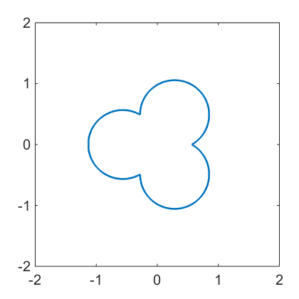
(a) Symmetric curvilinear triangle $\Omega$

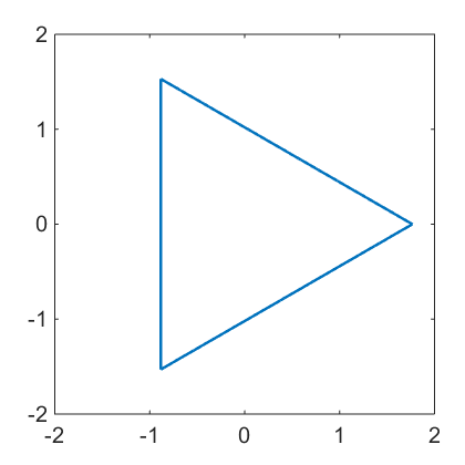
(b) Equilateral triangle $P=\Omega^{r}$

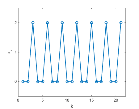
(c) Geometric factor $\sigma_{k}\left[\Omega\right]$

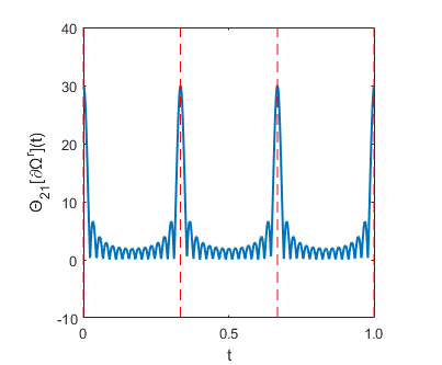
(d) Truncation of $\Theta[\partial\Omega^{r}]$

Figure 5.1: Symmetric cornered domain. (a) and (b) illustrate a curvilinear triangle $\Omega$ and its reflection $P$ across the unit circle. Since ${\Omega}$ is $3$-point radially symmetric, $\sigma_{k}[{\Omega}]=0$ for every $k\not\equiv 0\pmod{3}$ as shown in (c). The graph $\Theta_{21}[\partial\Omega^{r}]$ in (d) shows three isolated peaks, located on the red dashed vertical lines indicating $t$-values for which $\Phi[\Omega](e^{-2\pi t{\rm{i}}})$ are corner points of $\partial\Omega$.

$k$	$\sigma_{k}$	$k$	$\sigma_{k}$
$1$	$0$	$11$	$-1\times 10^{-15}$
$2$	$-3\times 10^{-17}$	$12$	$2.00000000001$
$3$	$1.999999999999994$	$13$	$1\times 10^{-15}$
$4$	$1\times 10^{-33}$	$14$	$1\times 10^{-16}$
$5$	$-3\times 10^{-16}$	$15$	$2.0000000001$
$6$	$1.99999999999997$	$16$	$8\times 10^{-16}$
$7$	$2\times 10^{-32}$	$17$	$-3\times 10^{-15}$
$8$	$-3\times 10^{-16}$	$18$	$2.000000001$
$9$	$2.0000000000003$	$19$	$-7\times 10^{-16}$
$10$	$4\times 10^{-16}$	$20$	$-7\times 10^{-15}$

Table 1: The 20 first geometric factors $\sigma_{k}$ of the symmetric domain in Figure 5.1(a), obtained from numerically computed GPTs. The values agree well with the analytic expression of (5.2).

5.3 Non-symmetric domain

In this example $\Omega$ is the non-symmetric domain with corners in Figure 5.2(a) (see Appendix B for the parametrization). As in Section 5.2, the GPTs are numerically computed and the geometric factors $\sigma_{k}$ are calculated from the GPTs via (2.2), (2.4), (2.17) and (2.19). Table 2 displays the first 20 geometric factors. Note that $\sigma_{k}\left[\Omega\right]$ shows an oscillatory behavior as $k$ increases, as also shown in Figure 5.2(c). The graph of $\Theta_{28}[\partial\Omega^{r}](t)$ shows three isolated peaks at the locations of the corner points, which are marked by red vertical lines. Again, the peaks correspond to the Dirac delta singularities in $\Theta$.

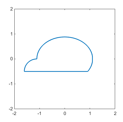
(a) Cap-shaped cornered domain $\Omega$

(b) Reflected domain $\Omega^{r}$

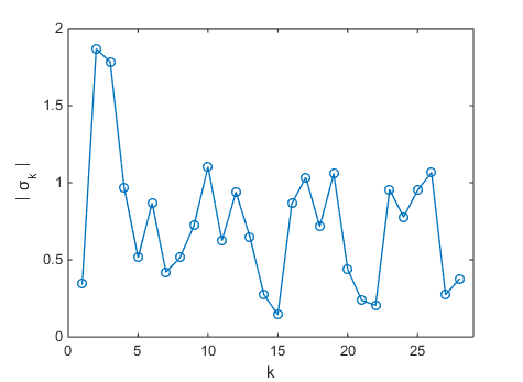
(c) Geometric factor $\sigma_{k}[\Omega]$

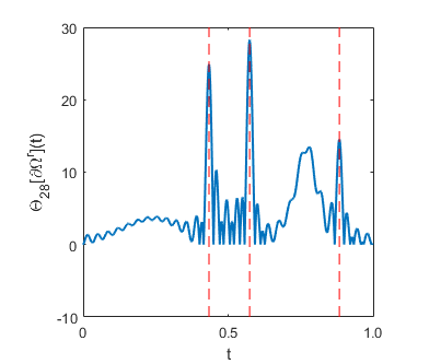
(d) Truncation of $\Theta[\partial\Omega^{r}]$

Figure 5.2: Non-symmetric cornered domain. (a) and (b) illustrate a non-symmetric domain $\Omega$ and its reflection $\Omega^{r}$ across the unit circle. (c) shows an oscillatory behavior of $\sigma_{k}[\Omega]$ as $k$ increases, which is consistent with Corollary 4.3. The graph $\Theta_{28}[\partial\Omega^{r}](t)$ in (d) shows three isolated peaks, located on the red dashed vertical lines indicating $t$-values for which $\Phi[\Omega](e^{-2\pi t{\rm{i}}})$ are corner points of $\partial\Omega$

$k$	$\sigma_{k}$	$k$	$\sigma_{k}$
$1$	$0.336144826114240-0.076400757440234{\rm i}$	$11$	$0.186721819078-0.595616065541{\rm i}$
$2$	$-1.75172536453942-0.64675188584893{\rm i}$	$12$	$0.023499384397+0.939740685579{\rm i}$
$3$	$0.03406793409600+1.78388113685821{\rm i}$	$13$	$0.49141111608-0.42493152167{\rm i}$
$4$	$0.82403911365013-0.50742133234639{\rm i}$	$14$	$0.14107795747-0.23706422509{\rm i}$
$5$	$0.49942961065065+0.12520990108117{\rm i}$	$15$	$-0.11870768404+0.08096200618{\rm i}$
$6$	$-0.1083287142652-0.8609605708526{\rm i}$	$16$	$0.0444798323-0.8639904912{\rm i}$
$7$	$-0.3918884064658-0.1538531930618{\rm i}$	$17$	$-0.6290121604+0.8209980128{\rm i}$
$8$	$-0.147595479311+0.493831447944{\rm i}$	$18$	$0.1981029905-0.6878495747{\rm i}$
$9$	$-0.072598481664-0.719868325959{\rm i}$	$19$	$-0.4512400133+0.9581338937{\rm i}$
$10$	$-0.330200317533+1.052309941949{\rm i}$	$20$	$0.407788339-0.162013757{\rm i}$

Table 2: The 20 first geometric factors $\sigma_{k}$ of the non-symmetric domain in Figure 5.2(a), obtained from numerically computed GPTs.

In Figure 5.3, we consider the imaging problem of $\Omega$ from a finite number of components of the GPTs. As discussed in Section 4.4 one can have the truncated series $\Phi_{N-2}[\Omega](\zeta)$ from $\left\{\gamma^{2}_{k1}:k\leq N\right\}$. In this example, we reconstruct $\Omega$ using $N=6$ and $N=29$. The image of the unit circle under $\Phi_{N-2}[\Omega]$ approximates the shape of $\partial\Omega$ even for small $N$. For $N=29$ the graph of $\Theta_{N-1}[\partial\Omega^{r}](t)$ shows isolated peaks at $t$ corresponding to corner points, while it does not for $N=6$.

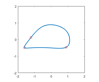
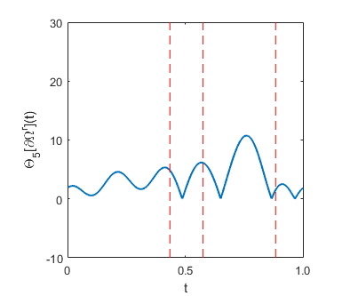
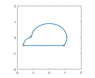
Figure 5.3: Imaging $\Omega$ from a finite number of components of the GPTs. $\Omega$ is given as in Figure 5.2(a) and $\left\{\gamma^{2}_{k1}:k\leq N\right\}$ are used with $N=6$ (top) and $N=29$ (bottom). The left column shows the images of the unit circle under $\Phi_{N-2}[\Omega]$. The small red circles indicate values of $\Phi_{N-2}[\Omega](e^{-2\pi t_{0}{\rm{i}}})$ for which $\Phi[\Omega](e^{-2\pi t_{0}{\rm{i}}})$ are corner points of $\partial\Omega$. The right column illustrates $\Theta_{N-1}[\partial\Omega^{r}]$. For small $N$ there is no isolated peak for $\Theta_{N-1}[\partial\Omega^{r}]$.

5.4 Smooth domain

In Figure 5.4 we consider a smooth domain, denoted by $\widetilde{\Omega}$, with $3$-point radial symmetry. Note that $\widetilde{\Omega}$ has a similar shape as that of $\Omega$ in Figure 5.1. In Figure 5.5 we consider another smooth domain, denoted again by $\widetilde{\Omega}$, which has a similar shape as $\Omega$ in Figure 5.2.

In both cases the domain $\widetilde{\Omega}$ is made as $\partial\widetilde{\Omega}=\{P(z):|z|=1\}$ by using a polynomial $P(z)$. Then, the corresponding geometric factors are analytically calculated. In contrast to the examples with the cornered domain, the geometric factors of $\widetilde{\Omega}$ decay exponentially. The partial sums of Fourier series of $\Theta$ have relatively large values at $t$-values corresponding to boundary points of $\widetilde{\Omega}^{r}$ with large curvature.

Since $\widetilde{\Omega}$ in Figure 5.4 is $3$-point radially symmetric, we have $\sigma_{k}[\widetilde{\Omega}]=0$ for every $k\not\equiv 0\pmod{3}$.

(a) Symmetric smooth domain $\widetilde{\Omega}$

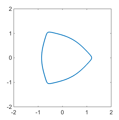
(b) Reflected domain ${\widetilde{\Omega}}^{r}$

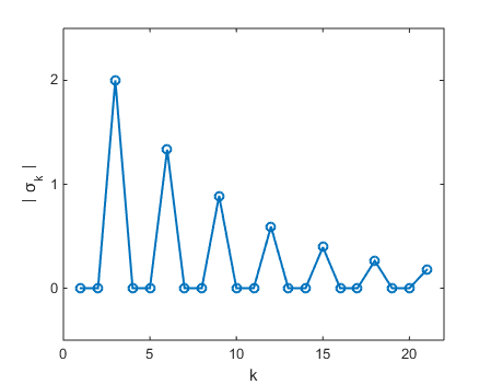
(c) Geometric factor $\sigma_{k}[\widetilde{\Omega}]$

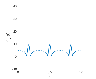
(d) Truncation of $\Theta[\partial\widetilde{\Omega}^{r}]$

Figure 5.4: Symmetric smooth domain. (a) and (b) illustrate a smooth domain $\widetilde{\Omega}$ and its reflection $\widetilde{\Omega}^{r}$ across the unit circle. (c) shows the exponential decay of $\sigma_{k}$ as $k$ increases. Since $\widetilde{\Omega}$ is $3$-point radially symmetric, $\sigma_{k}[\widetilde{\Omega}]=0$ for every $k\not\equiv 0\pmod{3}$. (d) shows the graph of a truncated Fourier series of $\Theta[\partial\Omega^{r}]$. $\Theta_{21}[\partial\widetilde{\Omega}^{r}]$ does not exhibit isolated peaks, but has relatively large values at boundary points of $\widetilde{\Omega}^{r}$ with large curvature.

(a) Symmetric smooth domain $\widetilde{\Omega}$

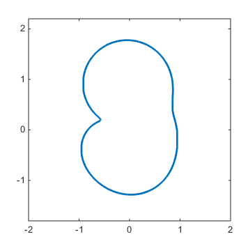
(b) Reflected domain ${\widetilde{\Omega}}^{r}$

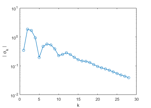
(c) Graph of $\sigma_{k}[\widetilde{\Omega}]$ in log scale

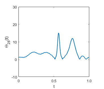
(d) Truncation of $\Theta[\partial\widetilde{\Omega}^{r}]$

Figure 5.5: Non-symmetric smooth domain. (a) and (b) illustrate a smooth domain $\widetilde{\Omega}$ and its reflection $\widetilde{\Omega}^{r}$ across the unit circle. (c) shows the exponential decay of $\sigma_{k}$ as $k$ increases. The graph of $\Theta_{28}[\partial\widetilde{\Omega}^{r}]$ in (d) does not exhibit isolated peaks, but has relatively large values at boundary points of $\widetilde{\Omega}^{r}$ with large curvature.

6 Proofs

6.1 Proof of Proposition 2.2

By (2.6), (2.8), and (2.9) and the definitions of $\mu_{n,k}$ and $b_{n,k}$, we have

$$\Phi(\zeta)^{n}-\sum_{m=1}^{\infty}\frac{\gamma_{mn}^{1}}{\Phi(\zeta)^{m}}=\Phi(\zeta)^{n}-\sum_{m=1}^{\infty}\gamma_{mn}^{1}S\Bigr{(}\frac{1}{\zeta}\Bigr{)}^{m}$$

$$=C^{n}\zeta^{2n}\Bigr{(}\sum_{k=1}^{\infty}\frac{\mu_{k-2}}{\zeta^{k}}\Bigr{)}^{n}-\sum_{m=1}^{\infty}\gamma_{mn}^{1}\frac{1}{C^{m}}\Bigr{(}\sum_{k=1}^{\infty}\frac{b_{k}}{\zeta^{k}}\Bigr{)}^{m}=C^{n}\sum_{k=n}^{\infty}\frac{\mu_{n,k}}{\zeta^{k-2n}}-\sum_{k=1}^{\infty}\Bigr{(}\sum_{m=1}^{k}\frac{1}{C^{m}}\gamma_{mn}^{1}b_{m,k}\Bigr{)}\frac{1}{\zeta^{k}}$$

$$=C^{n}\sum_{k=0}^{n}\mu_{n,2n-k}\zeta^{k}+\sum_{k=1}^{\infty}\Bigr{(}C^{n}\mu_{n,2n+k}-\sum_{m=1}^{k}\frac{1}{C^{m}}\gamma_{mn}^{1}b_{m,k}\Bigr{)}\frac{1}{\zeta^{k}}.$$ (6.1)

Note that

$$\Phi(\zeta)^{n}-\sum_{m=1}^{\infty}\frac{\gamma_{mn}^{1}}{\Phi(\zeta)^{m}}=\frac{1}{2}\left(V_{1}\circ\Phi+V_{2}\circ\Phi\right)(\zeta)$$

with $V_{1}$ and $V_{2}$ defined in Section 2.3. From Lemma 2.1, the right-hand side of the above equation has an entire extension. The main idea of the proof of Lemma 2.1 is the equality

$$-\frac{1}{2}{\left(V_{1}\circ\Phi+V_{2}\circ\Phi\right)(\zeta)} =\mbox{const.}-\frac{1}{2}\overline{\left(V_{1}\circ\Phi-V_{2}\circ\Phi\right)(\zeta)}$$ (6.2)

$$=\mbox{const.}-\frac{1}{2}\overline{\left(V_{1}\circ\Phi-V_{2}\circ\Phi\right)(\frac{1}{\bar{\zeta}})}$$

on $|\zeta|=1$ due to (2.11) and (2.12). Since the last term in the above equation is analytic for $|\zeta|<1$, the function $\frac{1}{2}{\left(V_{1}\circ\Phi+V_{2}\circ\Phi\right)(\zeta)}$ has an entire extension. Therefore, the principal parts of (6.1) should vanish:

$$C^{n}\mu_{n,2n+k}-\sum_{m=1}^{k}\frac{1}{C^{m}}\gamma_{mn}^{1}b_{m,k}=0.$$ (6.3)

Rearranging (6.3), and since $b_{k,k}=1$, we get $\gamma_{kn}^{1}=C^{k+n}\Bigr{(}\mu_{n,2n+k}-\sum_{m=1}^{k-1}\frac{1}{C^{m+n}}\gamma_{mn}^{1}b_{m,k}\Bigr{)}$ for each $n,k\in\mathbb{N}$. This proves (2.14).

From (6.2), for each $k\in\mathbb{N}\cup\{0\}$ and sufficiently large $R>0$ we have

$$\int_{|\zeta|=1}-\frac{1}{2}{\left(V_{1}\circ\Phi-V_{2}\circ\Phi\right)(\zeta)}\,\zeta^{k}d\zeta=\int_{|\zeta|=1}\overline{-\frac{1}{2}{\left(V_{1}\circ\Phi+V_{2}\circ\Phi\right)(\zeta)}}\,\zeta^{k}d\zeta$$

$$=\int_{|\zeta|=1}\overline{-\frac{1}{2}{\left(V_{1}\circ\Phi+V_{2}\circ\Phi\right)(\bar{\zeta}^{-1})}}\,\zeta^{k}d\zeta=\int_{|\zeta|=\frac{1}{R}}\overline{-\frac{1}{2}{\left(V_{1}\circ\Phi+V_{2}\circ\Phi\right)(\bar{\zeta}^{-1})}}\,\zeta^{k}d\zeta$$

$$=-\int_{|\zeta|=\frac{1}{R}}\overline{\Phi(\bar{\zeta}^{-1})^{n}-\sum_{m=1}^{\infty}\frac{\gamma_{mn}^{1}}{\Phi(\bar{\zeta}^{-1})^{m}}}\,\zeta^{k}d\zeta,$$ (6.4)

and the left-hand side equals

$$\int_{|\zeta|=1}-\frac{1}{2}{\left(V_{1}\circ\Phi-V_{2}\circ\Phi\right)(\zeta)}\,\zeta^{k}d\zeta=\int_{|\zeta|=R}\left(\sum_{m=1}^{\infty}\frac{\gamma_{mn}^{2}}{\Phi(\zeta)^{m}}\right)\zeta^{k}d\zeta.$$ (6.5)

We compute

$$\overline{\Phi(\bar{\zeta}^{-1})^{n}-\sum_{m=1}^{\infty}\frac{\gamma_{mn}^{1}}{\Phi(\bar{\zeta}^{-1})^{m}}} =\overline{\Phi(\bar{\zeta}^{-1})^{n}}-\overline{\sum_{m=1}^{\infty}{\gamma_{mn}^{1}}{S(\bar{\zeta})^{m}}}$$

$$={C}^{n}\Bigr{(}\sum_{k=-1}^{\infty}\overline{\mu_{k}}\zeta^{k}\Bigr{)}^{n}-\sum_{m=1}^{\infty}\overline{\gamma_{mn}^{1}}\frac{1}{{C}^{m}}\Bigr{(}\sum_{k=1}^{\infty}\overline{b_{k}}\zeta^{k}\Bigr{)}^{m}\quad\mbox{on }|\zeta|=\frac{1}{R},$$ (6.6)

and

$$\sum_{m=1}^{\infty}\frac{\gamma_{mn}^{2}}{\Phi(\zeta)^{m}}=\sum_{m=1}^{\infty}\gamma_{mn}^{2}S(\frac{1}{\zeta})^{m}=\sum_{m=1}^{\infty}\gamma_{mn}^{2}\frac{1}{C^{m}}\Bigr{(}\sum_{k=1}^{\infty}\frac{b_{k}}{\zeta^{k}}\Bigr{)}^{m}\quad\mbox{on }|\zeta|=R.$$ (6.7)

By applying a similar multinomial expansion as in (6.1), we can formally expand the summation of two components in (6.6) and (6.7) which contain principal parts:

$$\sum_{m=1}^{\infty}\gamma_{mn}^{2}\frac{1}{C^{m}}\Bigr{(}\sum_{k=1}^{\infty}\frac{b_{k}}{\zeta^{k}}\Bigr{)}^{m}+{C}^{n}\Bigr{(}\sum_{k=-1}^{\infty}\overline{\mu_{k}}\zeta^{k}\Bigr{)}^{n}$$

$$= \sum_{k=1}^{\infty}\Bigr{(}\sum_{m=1}^{k}\frac{1}{C^{m}}\gamma_{mn}^{2}b_{m,k}\Bigr{)}\frac{1}{\zeta^{k}}+{C}^{n}\sum_{k=n}^{\infty}\overline{\mu_{n,k}}\zeta^{k-2n}$$

$$= {C}^{n}\sum_{k=0}^{\infty}\overline{\mu_{n,2n+k}}\zeta^{k}+\sum_{k=1}^{n}\Bigr{(}{C}^{n}\overline{\mu_{n,2n-k}}+\sum_{m=1}^{k}\frac{1}{C^{m}}\gamma_{mn}^{2}b_{m,k}\Bigr{)}\frac{1}{\zeta^{k}}+\sum_{k=n+1}^{\infty}\Bigr{(}\sum_{m=1}^{k}\frac{1}{C^{m}}\gamma_{mn}^{2}b_{m,k}\Bigr{)}\frac{1}{\zeta^{k}}.$$

In view of (6.4) and (6.5), the principal parts of the above equation should vanish:

$$\begin{cases}{C}^{n}\overline{\mu_{n,2n-k}}+\sum_{m=1}^{k}\frac{1}{C^{m}}\gamma_{mn}^{2}b_{m,k}=0,&\mbox{for }1\leq k\leq n,\\ \sum_{m=1}^{k}\frac{1}{C^{m}}\gamma_{mn}^{2}b_{m,k}=0,&\mbox{for }k\geq n+1.\end{cases}$$

Rearranging the above equation, and since $b_{k,k}=1$, we get

$$\gamma_{kn}^{2}=\begin{cases}-C^{k+n}\Bigr{(}\overline{\mu_{n,2n-k}}+\sum_{m=1}^{k-1}\frac{1}{C^{m+n}}\gamma_{mn}^{2}b_{m,k}\Bigr{)},&\mbox{for }1\leq k\leq n,\\ -C^{k+n}\sum_{m=1}^{k-1}\frac{1}{C^{m+n}}\gamma_{mn}^{2}b_{m,k},&\mbox{for }k\geq n+1,\end{cases}$$

This proves (2.15). ∎

6.2 Proofs of Proposition 2.3 and Remark 1

Proof of Proposition 2.3 From (2.15) with $n=k=1$ and (2.13), we have $\gamma_{11}^{2}=-C^{2}\overline{\mu_{1,1}}=-C^{2}.$ This implies (2.16). Applying again (2.15) for $n=1$ and $k\geq 2$, we have $\gamma_{k1}^{2}=-C^{k+1}\sum_{m=1}^{k-1}\frac{\gamma_{m1}^{2}}{C^{m+1}}b_{m,k},$ which is equivalent to $\sum_{m=1}^{k}\frac{\gamma_{m1}^{2}}{C^{m+1}}b_{m,k}=0$. Hence we have for $k\geq 2$,

$$0=\sum_{m=1}^{k}\frac{\gamma_{m1}^{2}}{C^{m+1}}b_{m,k}=\frac{\gamma_{11}^{2}}{C^{2}}b_{1,k}+\sum_{m=2}^{k}\frac{\gamma_{m1}^{2}}{C^{m+1}}b_{m,k}=-b_{k}+\sum_{m=2}^{k}\frac{\gamma_{m1}^{2}}{C^{m+1}}b_{m,k}\,.$$

This proves (2.17). ∎

Proof of Remark 1 From (2.14), we have

$$\gamma_{k1}^{1}=C^{k+1}\Bigr{(}\mu_{1,2+k}-\sum_{m=1}^{k-1}\frac{\gamma_{m1}^{1}}{C^{m+1}}b_{m,k}\Bigr{)},\quad\mbox{for }k\geq 2.$$

It follows that $\mu_{1,2+k}=\sum_{m=1}^{k-1}\frac{\gamma_{m1}^{1}}{C^{m+1}}b_{m,k}+\frac{\gamma_{k1}^{1}}{C^{k+1}}=\sum_{m=1}^{k}\frac{\gamma_{m1}^{1}}{C^{m+1}}b_{m,k}$ because $b_{k,k}=1$. Hence, for $k\geq 2$, we have

$$\mu_{k}=\mu_{1,2+k}=\sum_{m=1}^{k}\frac{\gamma_{m1}^{1}}{C^{m+1}}b_{m,k}=\frac{\gamma_{11}^{1}}{C^{2}}b_{k}+\sum_{m=2}^{k}\frac{\gamma_{m1}^{1}}{C^{m+1}}b_{m,k}\,,$$

where $C$ is as in (2.16). This proves (2.18). ∎

7 Conclusions

We have analyzed the effects of corners of an insulating inclusion $\Omega$ on the perturbation of an electric potential. We derived explicit connections between generalized polarization tensors and coefficients of interior Riemann mapping functions on the way. We defined a sequence of geometric factors using these mapping coefficients. Mutually equivalent relations are then deduced between GPTs, the Riemann mapping coefficients, and the geometric factors. We finally characterized the corner effect: the sequence of geometric factors is the sequence of Fourier coefficients of the generalized external angle function for $\Omega^{r}$, the reflection of $\Omega$ across the unit circle, where the generalized external angle function contains the Dirac delta singularity at the corner points. Based on this corner effect, we established a criteria for the existence of corner points on the inclusion boundary in terms of the geometric factors. We assumed that the inclusion is insulated. It will be of interest to find geometric factors for inclusions with arbitrary conductivity that reveal the presence of corners.

Appendix A Carathéodory’s mapping theorem

For the relation between the convergence of domains and the convergence of the corresponding conformal mappings, we introduce some content from [26].

Definition 1.

Let $\{\Omega_{n}\}_{n\in\mathbb{N}}$ be a sequence of simply connected and uniformly bounded domains in $\mathbb{C}$, and each $\Omega_{n}$ contains a fixed disk centered at $z_{0}$. The ${kernel}$ of $\{\Omega_{n}\}_{n\in\mathbb{N}}$ is defined as the largest open domain $\Omega_{z_{0}}$ containing $z_{0}$ such that every compact subset $K\subset\Omega_{z_{0}}$ belongs to $\Omega_{n}$ for all $n\geq N$ with some $N\in\mathbb{N}$ depending on $K$.

Definition 2 (Kernel convergence in the sense of Carathéodory).

Let $G_{z_{0}}$ be a kernel of $\{\Omega_{n}\}_{n\in\mathbb{N}}$ relative to the point $z_{0}$. If every subsequence of $\{\Omega_{n}\}_{n\in\mathbb{N}}$ has the same kernel $\Omega_{z_{0}}$, then $\Omega_{n}$ is said to converge to $\Omega_{z_{0}}$. Otherwise, $\Omega_{n}$ is said to diverge.

We defined a concept of convergence in the sense of Carathéodory. Now, let’s see how the convergence in the sense of Carathéodory is related to the convergence of the function sequences.

Theorem A.1 (Carathéodory’s mapping theorem).

For each $n\in\mathbb{N}$, let $f_{n}:\Omega_{n}\to\mathbb{D}$ be a conformal mapping that satisfies

$$f_{n}(z_{0})=0,\quad f^{\prime}_{n}(z_{0})>0.$$

Similarly, let $f:\Omega_{z_{0}}\to\mathbb{D}$ be a conformal mapping that satisfies

$$f(z_{0})=0,\quad f^{\prime}(z_{0})>0.$$

If $\Omega_{n}$ converges to $\Omega_{z_{0}}$, then $f_{n}$ converges uniformly to $f$ inside $\Omega_{z_{0}}$ (which means by definition that $f_{n}$ converges uniformly on any compact subset of $\Omega_{z_{0}}$), and $f_{n}^{-1}$ converges uniformly to $f^{-1}$ inside $\mathbb{D}$. Conversely, if $f_{n}$ converges uniformly to $f$ inside $\Omega_{z_{0}}$, or if $f_{n}^{-1}$ converges uniformly to $f^{-1}$ inside $\mathbb{D}$, then $\Omega_{n}$ converges to $\Omega_{z_{0}}$.

Appendix B Parametrization of the non-symmetric domain in Section 5.3

The boundary of the non-symmetric domain $\Omega$ in Section 5.3 can be parametrized as follows:

$$\gamma(t)=\begin{cases}\left(-\frac{1}{2}\sin\left(4\pi ct\right)-\frac{\sqrt{2}\pi}{4},\quad-\frac{1}{2}+\frac{1}{2}\cos\left(4\pi ct\right)\right),\quad t\in[0,t_{1}],\\[5.69054pt] \left(2\pi c(t-t_{2})-\sqrt{2}\arcsin\left(\frac{\sqrt{2}}{2}\cos(2\pi a)\right),\quad-\frac{1}{2}\right),\quad t\in[t_{1},t_{2}],\\[5.69054pt] \left(-\sqrt{2}\arcsin\left(\frac{\sqrt{2}}{2}\cos\left(2\pi c(t-t_{2})+2\pi a\right)\right),\quad-\operatorname{arcsinh}\left(\sin\left(2\pi c(t-t_{2})+2\pi a\right)\right)\right),\quad t\in[t_{2},1],\end{cases}$$

with $a=\frac{1}{2}-\frac{1}{2\pi}\arcsin\left(\sinh\left(\frac{1}{2}\right)\right)$, $b=a-\frac{1}{4\pi}-\frac{\sqrt{2}}{8}+\frac{\sqrt{2}}{2\pi}\arcsin\left(\frac{\sqrt{2}}{2}\cos(2\pi a)\right)$, $c=\frac{9}{8}-b$, $t_{1}=\frac{1}{8c}\approx 0.1122$, and $t_{2}=t_{1}+\left(\frac{a-b}{c}\right)\approx 0.4731.$

References

- [1] Habib Ammari, Giulio Ciraolo, Hyeonbae Kang, Hyundae Lee, and Graeme W Milton. Spectral theory of a Neumann-Poincaré-type operator and analysis of cloaking due to anomalous localized resonance. Archive for Rational Mechanics and Analysis, 208(2):667–692, 2013.
- [2] Habib Ammari, Thomas Boulier, Josselin Garnier, Wenjia Jing, Hyeonbae Kang, and Han Wang. Target identification using dictionary matching of generalized polarization tensors, Foundations of Computational Mathematics, 14(1):27–62, 2014.
- [3] Habib Ammari, Josselin Garnier, Wenjia Jing, Hyeonbae Kang, Mikyoung Lim, Knut Sølna, and Han Wang. Mathematical and Statistical Methods for Multistatic Imaging, volume 2098. Springer, 2013.
- [4] Habib Ammari, Josselin Garnier, Hyeonbae Kang, Mikyoung Lim, and Sanghyeon Yu. Generalized polarization tensors for shape description. Numerische Mathematik, 126(2):199–224, 2014.
- [5] Habib Ammari and Hyeonbae Kang. Reconstruction of Small Inhomogeneities from Boundary Measurements. Springer, 2004.
- [6] Habib Ammari and Hyeonbae Kang. Polarization and Moment Tensors: With Applications to Inverse Problems and Effective Medium Theory, volume 162. Springer Science & Business Media, 2007.
- [7] Habib Ammari, Hyeonbae Kang, Hyundae Lee, and Mikyoung Lim. Enhancement of near cloaking using generalized polarization tensors vanishing structures. Part I: The conductivity problem. Communications in Mathematical Physics, pages 1–14, 2013.
- [8] Habib Ammari, Hyeonbae Kang, Hyundae Lee, Mikyoung Lim, and Sanghyeon Yu. Enhancement of near cloaking for the full Maxwell equations. SIAM Journal on Applied Mathematics, 73(6):2055–2076, 2013.
- [9] Habib Ammari, Hyeonbae Kang, Mikyoung Lim, and Habib Zribi. The generalized polarization tensors for resolved imaging. Part I: Shape reconstruction of a conductivity inclusion. Mathematics of Computation, 81(277):367–386, 2012.
- [10] Kendall E. Atkinson. The Numerical Solution of Integral Equations of the Second Kind, volume 4. Cambridge University Press, 1997.
- [11] Torsten Carleman. Über das Neumann-Poincarésche problem für ein Gebiet mit Ecken. 1916.
- [12] S. Cho and S.R. Pai. On the regularity of the Riemann mapping function in the plane. Pusan Kyongnam Math. J, 12(2):203–211, 1996.
- [13] A. Clebsch, C. Neumann, F. Klein, A. Mayer, D. Hilbert, O. Blumenthal, A. Einstein, C. Carathéodory, E. Hecke, B.L. Waerden, et al. Mathematische Annalen. Number V. 104. J. Springer, 1931.
- [14] Tobin A. Driscoll and Lloyd N. Trefethen. Schwarz-Christoffel Mapping, volume 8. Cambridge University Press, 2002.
- [15] L. Escauriaza, E. B. Fabes, and G. Verchota. On a regularity theorem for weak solutions to transmission problems with internal Lipschitz boundaries. Proceedings of the American Mathematical Society, 115(4):1069–1076, 1992.
- [16] Johan Helsing. Solving integral equations on piecewise smooth boundaries using the RCIP method: a tutorial. arXiv:1207.6737 [physics.comp-ph], revised 2017.
- [17] Johan Helsing, Hyeonbae Kang, and Mikyoung Lim. Classification of spectra of the Neumann-Poincaré operator on planar domains with corners by resonance. Annales de l’Institut Henri Poincaré (C) Non Linear Analysis, 34(4):991 – 1011, 2017.
- [18] Johan Helsing and Anders Karlsson. Determination of normalized electric eigenfields in microwave cavities with sharp edges. Journal of Computational Physics, 304:465–486, 2016.
- [19] Johan Helsing, Ross C. McPhedran, and Graeme W. Milton. Spectral super-resolution in metamaterial composites. New Journal of Physics, 13(11):115005, 2011.
- [20] Johan Helsing and Rikard Ojala. Corner singularities for elliptic problems: Integral equations, graded meshes, quadrature, and compressed inverse preconditioning. Journal of Computational Physics, 227(20):8820–8840, 2008.
- [21] Johan Helsing and Karl-Mikael Perfekt. On the polarizability and capacitance of the cube. Applied and Computational Harmonic Analysis, 34(3):445–468, 2013.
- [22] Masaru Ikehata. Enclosing a polygonal cavity in a two-dimensional bounded domain from Cauchy data. Inverse Problems, 15(5):1231, 1999.
- [23] Hyeonbae Kang, Hyundae Lee, and Mikyoung Lim. Construction of conformal mappings by generalized polarization tensors. Mathematical Methods in the Applied Sciences, 38(9):1847–1854, 2015.
- [24] Hyeonbae Kang, Mikyoung Lim, and Sanghyeon Yu. Spectral resolution of the Neumann-Poincaré operator on intersecting disks and analysis of plasmon resonance. Archive for Rational Mechanics and Analysis, pages 1–33, 2015.
- [25] Hyeonbae Kang and KiHyun Yun. Optimal estimates of the field enhancement in presence of a bow-tie structure of perfectly conducting inclusions in two dimensions. arXiv preprint arXiv:1707.00098, 2017.
- [26] A. I. Markushevich. Theory of Functions of a Complex Variable. Vol. I, II, III. Chelsea Publishing Co., New York, English edition, 1977.
- [27] Karl-Mikael Perfekt and Mihai Putinar. The essential spectrum of the Neumann-Poincaré operator on a domain with corners. Archive for Rational Mechanics and Analysis, 223(2):1019–1033, 2017.
- [28] George Pólya and Gábor Szegő. Isoperimetric Inequalities in Mathematical Physics. Number 27. Princeton University Press, 1951.
- [29] Elias M. Stein and Rami Shakarchi. Princeton Lectures in Analysis. Princeton University Press, 2003.
- [30] Gregory Verchota. Layer potentials and regularity for the Dirichlet problem for Laplace’s equation in Lipschitz domains. Journal of Functional Analysis, 59(3):572–611, 1984.
- [31] S.E. Warschawski. On a theorem of L. Lichtenstein. Pacific Journal of Mathematics, 5(5):835–839, 1955.
- [32] Sanghyeon Yu and Mikyoung Lim. Shielding at a distance due to anomalous resonance. New Journal of Physics, 19(3):033018, 2017.