Linear stability analysis on the onset of viscous fingering due to a non monotonic viscosity profile for immiscible fluids

Abstract

The onset of viscous fingering in the presence of a non monotonic viscosity profile is investigated theoretically for two immiscible fluids. Classical fluid dynamics predicts that no unstable behavior may be observed when a viscous fluid pushes a less viscous one in a Hele-Shaw cell. Here, we show that the presence of a viscosity gradient at the interface between both fluids destabilize the interface facilitating the spread of the perturbation. The influence of the viscosity gradient on the dispersion relation is analyzed.

I Introduction

Saffman-Taylor instability Taylor58 may arise when two fluids of different viscosity are pushed by a pressure gradient through two plane parallel plates (Hele Shaw cell). It is well known, both experimentally and theoretically, that when a less viscous Newtonian fluid displaces a more viscous one develop a fingering instability at the interface between both immiscible fluids Faber95 . For non Newtonian fluids, an unexpected propagation of fractures develop in the invaded fluid Nittmann85 ; Wilson90 ; Mora10 .

Recent experiments and numerical simulations have shown the possibility of viscous fingering in the presence of non monotonic viscosity profiles under stable conditions for miscible fluids. Destabilization of the interface of a viscous fluid displacing a less viscous one have been shown to occur in the presence of chemical reactions Riolfo12 , for a non-ideal water-alcohol mixture Haudin16 , or for differential diffusion of two species Mishra10 . Theoretical predictions of this behavior for reacting miscible fluids show that even if the front is initially stable, reactions taking place at the interface may destabilize it Tan86 ; Manickam93 ; Schafroth07 ; Hejazi10 ; Nagatsu11 . In these papers, the existence of a chemical reaction at the interface proved to be necessary for the observed unstable behavior.

In this work, we present a linear stability analysis for the onset of viscous fingering for two immiscible fluids under stable conditions subject to a non monotonic viscosity profile.

II Theory

The equation of motion of an incompressible newtonian fluid is given by,

$$\rho\frac{Du_{i}}{Dt} = -\frac{\partial p}{\partial x_{i}}+\frac{\partial}{\partial x_{j}}\left(2\mu e_{ij}\right),$$ (1)

$$\frac{\partial u_{i}}{\partial x_{i}} = 0$$ (2)

where $D/Dt$ is the material derivative, $\rho$ is the constant density, $u_{i}$ the velocity field, $p$ the pressure, $\mu$ the dynamic viscosity, and $e_{ij}=(\partial u_{i}/\partial x_{j}+\partial u_{j}/\partial x_{i})/2$ is the strain rate tensor. For a non monotonic viscosity profile $\mu=\mu(x_{i})$, Eq. (1) becomes,

$$\rho\frac{Du_{i}}{Dt}=-\frac{\partial p}{\partial x_{i}}+\mu\frac{\partial^{2}u_{i}}{\partial x_{j}\partial x_{j}}+2e_{ij}\frac{\partial\mu}{\partial x_{j}}$$ (3)

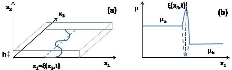
Figure 1: Sketch of the Hele-Shaw cell (a) and both viscosity profiles $\mu(x_{1})$ (b) used here (continuous and dashed lines near the interface).

We consider the case where a viscous fluid is pushing a less viscous one in the $x_{1}$-direction between closely spaced parallel plates separated some distance $h$ as it is shown in Fig. 1(a), subject to a perturbation at the interface $x_{1}=\xi(x_{3},t)$. In the basic Hele-Shaw flow, we suppose a negative pressure gradient along the $x_{1}$ axis so that the flow goes from the left ($x_{1}<0$) to the right ($x_{1}>0$). The velocity field is $[u_{1}^{0}(x_{2}),0,0]$. The interface between the two fluids is $x_{1}=\xi^{0}(t)$ with $\xi^{0}(t)=\langle u_{1}^{0}(x_{2})\rangle t$. Following the standard decomposition in normal modes, we perturb the system of equations (3). Thus, the perturbed velocity field is $[u_{1}^{0}(x_{2})+\epsilon u_{1}^{1}(x_{i},t),0,\epsilon u_{3}^{1}(x_{i},t)]$, the pressure $P^{0}+\epsilon P^{1}(x_{i},t)$, and the interface equation is $x_{1}=\xi^{0}(t)+\epsilon\xi^{1}(x_{3},t)$. Assuming a sinusoidal perturbation along the $x_{3}$ axis, the perturbed quantities can be written as,

$$\xi^{1}(x_{3},t) = \xi\cos(k_{3}x_{3})\exp(\omega t)$$

$$u_{1}^{1}(x_{i},t) = u_{a,b}(x_{2})\cos(k_{3}x_{3})$$

$$\exp\left(\omega t\pm k_{1}[x_{1}-\xi^{0}(t)]\right)$$

$$u_{3}^{1}(x_{i},t) = w_{a,b}(x_{2})\cos(k_{3}x_{3})$$

$$\exp\left(\omega t\pm k_{1}[x_{1}-\xi^{0}(t)]\right)$$

$$P^{1}(x_{1},x_{3},t) = P_{a,b}\cos(k_{3}x_{3})\exp\left(\omega t\pm k_{1}[x_{1}-\xi^{0}(t)]\right)$$

where $\pm$ stands for the left (a) and right (b) fluids with viscosities $\mu_{a}>\mu_{b}$, respectively. $\xi$, $u(x_{2})$, $w(x_{2})$, and $P$ are the amplitudes of the normal modes of the perturbation. The problem is completed by the no-slip boundary condition at the plates $u_{i}=0$ for $x_{2}=0,h$. Without loss of generality, from now on, we assume the viscosity profile $\mu=\mu(x_{1})$.

Rewriting Eq. (3) at zero order in $\epsilon$ we obtain the Darcy’s law,

$$u_{1}^{0}(x_{2})=\frac{G}{2\mu}\left(x_{2}^{2}-hx_{2}\right)$$ (4)

with $G$ the negative gradient along the $x_{1}$ axis. The mean velocity $\langle u_{1}^{0}\rangle=-Gh^{2}/12\mu$.

At first order in $\epsilon$, the amplitude of the normal mode $u_{a,b}$ is given by,

$$\mu_{a,b}\frac{d^{2}u_{a,b}}{dx_{2}^{2}}-\Phi_{a,b}(x_{2})u_{a,b}=\mp k_{1}P_{a,b}$$ (5)

and

$$\Phi_{a,b}(x_{2}) = \rho_{a,b}\omega\mp\rho_{a,b}k_{1}\langle u_{1}^{0}\rangle\pm\rho_{a,b}k_{1}u_{1}^{0}(x_{2})$$ (6)

$$-\mu_{a,b}(k_{1}^{2}-k_{3}^{2})\mp 2k_{1}\frac{\partial\mu_{a,b}}{\partial x_{1}}$$

A similar equation can be obtained for the mode $w_{a,b}$.

Two conditions must be imposed at the interface, namely the kinematical condition and the condition of continuity of normal stress, both averaged with respect to $x_{2}$,

$$\mid\langle u_{1}^{1}(x_{2})\rangle\mid_{a,b} = \frac{\partial\xi^{1}}{\partial t},$$

$$P^{1}_{a}-P^{1}_{b} = -\gamma\frac{\partial^{2}\xi^{1}}{\partial x_{3}^{2}}$$ (7)

where $\gamma$ is the surface tension at the interface.

Then, the set of equations (5-7) is solved by employing a shooting scheme. Fig. 1(b) summarizes the two non monotonic viscosity profiles used in our simulations. In both cases, the profile exhibits a maximum or a minimum of viscosity on the interface between both fluids.

III Results

Numerical simulations were performed for a silicone oil invading a Hele-Shaw cell filled with water at constant velocity. For both viscosity profiles, $\omega$ is always negative for any wave number k (vector with components $k_{1}$ and $k_{3}$ in the plane ($x_{1},x_{3}$)). Thus, in terms of classical fluid physics, the interface between the two fluids should be stable under perturbations. The average values $\langle u_{1}^{1}(x_{2})\rangle_{a,b}$ have opposite signs below some critical wave number $k_{c}$ indicating that perturbations annihilate at both sides of the interface. For $k>k_{c}$, perturbations grow in the $x_{1}$ direction, destabilizing the interface. Figure 2 shows the dispersion relation $\omega(k_{c})$ which is qualitatively the same for the two viscosity profiles used here. Thus, viscous fingering develops but contrary to the unstable case where a low viscous fluid invades a high viscous one, the extent of the fingers is attenuated by the term $\exp(-\omega t)$.

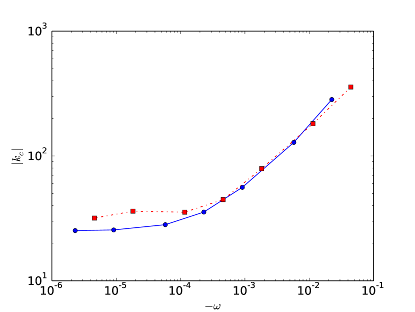
Figure 2: Dispersion relation, $k_{c}(\omega)$ for two values of the viscosity gradient at the interface; $\partial\mu/\partial x_{1}=1$ (blue dots) and $\partial\mu/\partial x_{1}=10$ (red squares). Set of parameters: $h=0.002$ m, Rhodorsil oil 47V500 ($\mu_{a}=0.485$ Pa s, $\rho_{a}=970$ kg/m³), water ($\mu_{b}=0.896\cdot 10^{-3}$ Pa s, $\rho_{b}=997$ kg/m³), and $\gamma=0.021$ N/m.

The critical wave number as a function of the viscosity gradient on the interface $|\partial\mu/\partial x_{1}|$ is shown in Fig. 3 for both viscosity profiles. Note that as the viscosity gradient increases, smaller/larger perturbations are needed in order to destabilize the flow depending on the presence of a maximum or a minimum of viscosity, respectively. This result also indicates that for equal amplitudes of the viscosity extremum on the interface, the instability develops more easily (larger $|\textbf{k}|$) for a viscosity maximum value.

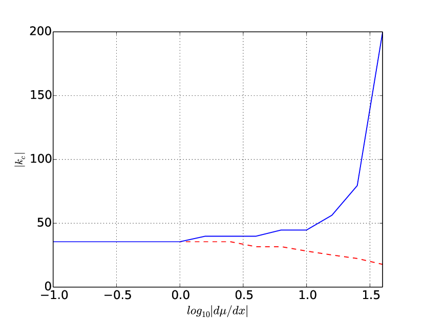
Figure 3: Critical wave number as a function of the viscosity gradient on the interface for a viscosity profile with a maximum (continuous line) and with a minimum (dashed line). $k_{1}=k_{3}$ and rest of parameters as in Fig. 2.

To deepen in this behavior, the invading fluid viscosity $\mu_{a}$ was varied while keeping constant $\partial\mu/\partial x_{1}$ on the interface as well as $\mu_{b}$. Increasing $\mu_{a}$ has a destabilizing effect as $-\omega$ diminishes, as it is shown in Fig. 4 for both profiles with opposite extremum. In other words, for the same perturbation ($k_{1},k_{3}$), the interface destabilize faster for larger values of $\mu_{a}$. The presence of a minimum in the viscosity profile also favors the destabilization of the interface, $\exp(-\omega_{min}t)>\exp(-\omega_{max}t)$, at constant $t$ and same perturbation; i.e. the system is more unstable when the viscosity profile has a minimum rather than a maximum.

Finally, considering small disturbances in the viscosity profile along the $x_{3}$-axis, the equations for the mode amplitudes $u$ and $w$ are coupled. Using the continuity equation $k_{1}u=k_{3}w$ uncouples them, and Eq. (6) becomes,

$$\Phi_{a,b}(x_{2}) = \rho_{a,b}\omega\mp\rho_{a,b}k_{1}\langle u_{1}^{0}\rangle\pm\rho_{a,b}k_{1}u_{1}^{0}(x_{2})$$ (8)

$$-\mu_{a,b}(k_{1}^{2}-k_{3}^{2})\mp 2k_{1}\frac{\partial\mu_{a,b}}{\partial x_{1}}$$

$$+\left(\frac{k_{3}^{2}\pm k_{1}^{2}}{k_{3}}\right)\frac{\partial\mu_{a,b}}{\partial x_{3}}$$

where $\partial\mu_{a,b}/\partial x_{3}$ must be evaluated on the interface. For small disturbances in the viscous profile on $x_{1}=\xi(x_{3},t)$, the contribution of the new term in (8) is small and the main results shown above hold.

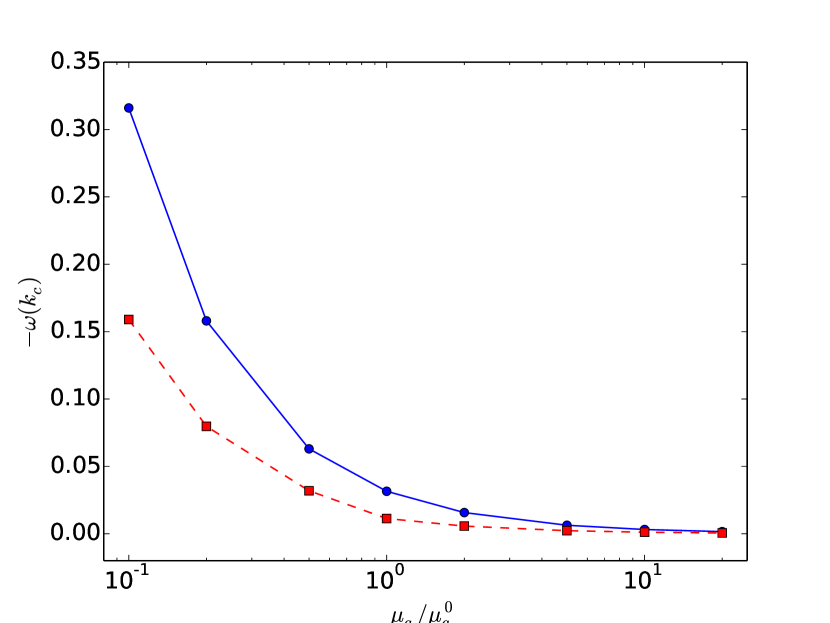
Figure 4: Influence of the invading fluid viscosity $\mu_{a}/\mu_{a}^{0}$ on the growth rate $\omega(k_{c})$ for a viscosity profile with a maximum on the interface (blue dots) and with a minimum (red squares and dashed line). $k_{1}=0.1k_{3}$, $\partial\mu/\partial x_{1}=10$, and $\mu_{a}^{0}$ is the silicone oil viscosity used in Fig. 2.

IV Conclusions

The onset condition of viscous fingering for a fluid displacing a less viscous one in a Hele-Shaw cell has been studied in the presence of a non monotonic viscosity profile in the direction of motion. For wave numbers above a critical one, perturbations at both sides of the interface spread in the same direction, destabilizing the interface. The spreading velocity is modulated by the term $\exp{(\omega t)}$ that attenuates the fingering in the direction of motion. This attenuation is larger when the viscosity profile has a maximum on the interface.

Our results are in agreement with theoretical calculations and experiments on miscible fluids with a reactive interface, but contrary to them, no chemical reactions are needed to account for the onset of viscous fingering under stable conditions. Recently, experiments by A. de Wit group Haudin16 have shown that the mixing length of this fingering zone was found to be smaller than for the unstable case (also analyzed simultaneously in their experiments). Similarly, for non-reactive viscous fingerings that develop between three finite slices Mishra08 , the extent of the fingers is also reduced under stable conditions. In our opinion, the observed mixing length reduction corresponds to the case solved here where the negative growth rate $\omega$ attenuates the perturbation growth.

Our results open new possibilities for experiments on viscous fingering under stable conditions in the presence of a non-monotonic viscosity profile for immiscible fluids.

V Acknowledgments

This work was financially supported by Ministerio de Economía y Competitividad and Xunta de Galicia (CGL2013-45932-R, GPC2015/014), and contributions by the COST Action MP1305 and CRETUS Strategic Partnership (AGRUP2015/02). All these programmes are co-funded by ERDF (EU).

References

- (1) G.I. Taylor and P.G. Saffman, Proc. R. Soc. London A 245, 312 (1958).
- (2) T.E. Faber. Fluid Dynamics for Physicists. (Cambridge Univ. Press, New York, 1995).
- (3) J. Nittmann, G. Daccord, and H. Stanley, Nature (London) 314, 141 (1985); J. Nase, A. Lindner, and C. Creton, Phys. Rev. Lett. 101, 074503 (2008).
- (4) S.D.R. Wilson, J. Fluid Mech. 220, 413–425 (1990).
- (5) S. Mora and M. Manna, Phys. Rev. E 81, 026305 (2010).
- (6) Y. Nagatsu, K. Matsuda, Y. Kato, and Y. Tada, J. Fluid Mech. 571, 475 (2007); L.A. Riolfo, Y. Nagatsu, S. Iwata, R. Maes, P.M.J. Trevelyan, and A. De Wit, Phys. Rev. E 85, 015304(R) (2012).
- (7) F. Haudin, M. Callewaert, W. De Malsche, and A. De Wit, Phys. Rev. Fluids 1, 074001 (2016).
- (8) M. Mishra, P.M.J. Trevelyan, C. Almarcha, and A. De Wit, Phys. Rev. Lett. 105, 204501 (2010).
- (9) C.T. Tan and G.M. Homsy, Phys. Fluids 29, 3549–3556 (1986).
- (10) O. Manickam and G.M. Homsy, Phys. of Fluids A 5, 1356–1357 (1993).
- (11) D. Schafroth, N. Goyal, E. Meiburg, Eur. J. Mech. B 26, 444–453 (2007).
- (12) S.H. Hejazi, P.M. Trevelyan, J. Azaiez, and A. De Wit, J. Fluid Mech. 652, 501–528 (2010).
- (13) Y. Nagatsu and A. De Wit, Phys. of Fluids 23, 043103 (2011).
- (14) M. Mishra, M. Martin, and A. De Wit, Phys. Rev. E 78, 066306 (2008).