The Refinement Calculus of Reactive Systems

Abstract

The Refinement Calculus of Reactive Systems (RCRS) is a compositional formal framework for modeling and reasoning about reactive systems. RCRS provides a language which allows to describe atomic components as symbolic transition systems or QLTL formulas, and composite components formed using three primitive composition operators: serial, parallel, and feedback. The semantics of the language is given in terms of monotonic property transformers, an extension to reactive systems of monotonic predicate transformers, which have been used to give compositional semantics to sequential programs. RCRS allows to specify both safety and liveness properties. It also allows to model input-output systems which are both non-deterministic and non-input-receptive (i.e., which may reject some inputs at some points in time), and can thus be seen as a behavioral type system. RCRS provides a set of techniques for symbolic computer-aided reasoning, including compositional static analysis and verification. RCRS comes with a publicly available implementation which includes a complete formalization of the RCRS theory in the Isabelle proof assistant.

1 Introduction

This paper presents the Refinement Calculus of Reactive Systems (RCRS), a comprehensive framework for compositional modeling of and reasoning about reactive systems. RCRS originates from the precursor theory of synchronous relational interfaces [78, 79], and builds upon the classic refinement calculus [10]. A number of conference publications on RCRS exist [66, 31, 67, 65, 33]. This paper collects some of these results and extends them in significant ways. The novel contributions of this paper and relation to our previous work are presented in §1.1.

The motivation for RCRS stems from the need for a compositional treatment of reactive systems. Generally speaking, compositionality is a divide-and-conquer principle. As systems grow in size, they grow in complexity. Therefore dealing with them in a monolithic manner becomes unmanageable. Compositionality comes to the rescue, and takes many forms. Many industrial-strength systems have employed for many years mechanisms for compositional modeling. An example is the Simulink tool from the Mathworks. Simulink is based on the widespread notation of hierarchical block diagrams. Such diagrams are both intuitive, and naturally compositional: a block can be refined into sub-blocks, sub-sub-blocks, and so on, creating hierarchical models of arbitrary depth. This allows the user to build large models (many thousands of blocks) while at the same time managing their complexity (at any level of the hierarchy, only a few blocks may be visible).

But Simulink’s compositionality has limitations, despite its hierarchical modeling approach. Even relatively simple problems, such as the problem of modular code generation (generating code for a block independently from context) require techniques not always available in standard code generators [53, 52]. Perhaps more serious, and more relevant in the context of this paper, is Simulink’s lack of formal semantics, and consequent lack of rigorous analysis techniques that can leverage the advances in the fields of computer-aided verification and programming languages.

RCRS provides a compositional formal semantics for Simulink in particular, and hierarchical block diagram notations in general, by building on well-established principles from the formal methods and programming language domains. In particular, RCRS relies on the notion of refinement (and its counterpart, abstraction) which are both fundamental in system design. Refinement is a binary relation between components, and ideally characterizes substitutability: the conditions under which some component can replace another component, without compromising the behavior of the overall system. RCRS refinement is compositional in the sense that it is preserved by composition: if $A^{\prime}$ refines $A$ and $B^{\prime}$ refines $B$, then the composition of $A^{\prime}$ and $B^{\prime}$ refines the composition of $A$ and $B$.

RCRS can be viewed as a refinement theory. It can also be viewed as a behavioral type system, similar to type systems for programming languages, but targeted to reactive systems. By behavioral we mean a type system that can capture not just data types of input and output ports of components (bool, int, etc.), but also complete specifications of the behavior of those components. As discussed more extensively in [79], such a behavioral type system has advantages over a full-blown verification system, as it is more lightweight: for instance, it allows type checking, which does not require the user to provide a formal specification of the properties that the model must satisfy, the model must simply type-check.

To achieve this, it is essential, as argued in [79], for the framework to be able to express non-input-receptive (also called non-input-enabled or non-input-complete) components, i.e., components that reject some input values. RCRS allows this. For example, a square-root component can be described in RCRS alternatively as: (1) a non-input-receptive component $C_{1}$ with input-output contract $x\geq 0\land y=\sqrt{x}$ (where $x,y$ are the input and output variables, respectively); or (2) an input-receptive component $C_{2}$ with contract $x\geq 0\to y=\sqrt{x}$. Simple examples of type-checking in the RCRS context are the following: Connecting the non-input-receptive square-root component $C_{1}$ to a component which outputs $x=-1$ results in a type error (incompatibility). Connecting $C_{1}$ to a non-deterministic component which outputs an arbitrary value for $x$ (this can be specified by the formula/contract $\mathit{true}$) also results in a type error. Yet, in both of the above cases $C_{2}$ will output a non-deterministically chosen value, even though the input constraint is not satisfied.

RCRS allows both non-input-receptive and non-deterministic components. This combination results in a game-theoretic interpretation of the composition operators, like in interface theories [22, 79]. Refinement also becomes game-theoretic, as in alternating refinement [7]. Game-theoretic composition can be used for an interesting form of type inference. For example, if we connect the non-input-receptive square-root component $C_{1}$ above to a non-deterministic component $C_{3}$ with input-output contract $x\geq u+1$ (where $x$ is the output of $C_{3}$, and $u$ its input), and apply the (game-theoretic) serial composition of RCRS, we obtain the condition $u\geq-1$ on the external input of the overall composition. The constraint $u\geq-1$ represents the weakest condition on $u$ which ensures compatibility of the connected components.

In a nutshell, RCRS consists of the following elements:

1. A modeling language (syntax), which allows to describe atomic components, and composite components formed by a small number of primitive composition operators (serial, parallel, and feedback). The language is described in §3.

2. A formal semantics, presented in §4. Component semantics are defined in terms of monotonic property transformers (MPTs). MPTs are extensions of monotonic predicate transformers used in theories of programming languages, and in particular in refinement calculus [10]. Predicate transformers transform sets of post-states (states reached by the program after its computation) into sets of pre-states (states where the program begins). Property transformers transform sets of a component’s output traces (infinite sequences of output values) into sets of input traces (infinite sequences of input values). Using this semantics we can express both safety and liveness properties.

3. A set of symbolic reasoning techniques, described in §5. In particular, RCRS offers techniques to

   • compute the symbolic representation of a composite component from the symbolic representations of its sub-components;

   • simplify composite components into atomic components;

   • reduce checking refinement between two components to checking satisfiability of certain logical formulas;

   • reduce input-receptiveness and compatibility checks to satisfiability;

   • compute the legal inputs of a component symbolically.

   We note that these techniques are for the most part logic-agnostic, in the sense that they do not depend on the particular logic used to represent components.

4. A toolset, described briefly in §6. The toolset consists mainly of:

   • a full implementation of the RCRS theory in the Isabelle proof assistant [61];

   • a translator of Simulink diagrams into RCRS code.

   Our implementation is open-source and publicly available from http://rcrs.cs.aalto.fi.

1.1 Novel contributions of this paper and relation to our prior work

Several of the ideas behind RCRS originated in the theory of synchronous relational interfaces [78, 79]. The main novel contributions of RCRS w.r.t. that theory are: (1) RCRS is based on the semantic foundation of monotonic property transformers, whereas relational interfaces are founded on relations; (2) RCRS can handle liveness properties, whereas relational interfaces can only handle safety; (3) RCRS has been completely formalized and most results reported in this and other RCRS papers have been proven in the Isabelle proof assistant; (4) RCRS comes with a publicly available toolset (http://rcrs.cs.aalto.fi) which includes the Isabelle formalization, a Translator of Simulink hierarchical block diagrams [31, 33], and a Formal Analyzer which performs, among other functions, compatibility checking, refinement checking, and automatic simplification of RCRS contracts.

RCRS was introduced in [66], which focuses on monotonic property transformers as a means to extend relational interfaces with liveness properties. [66] covers serial composition, but not parallel nor feedback. It also does not cover symbolic reasoning nor the RCRS implementation. Feedback is considered in [67], whose aim is in particular to study instantaneous feedback for non-deterministic and non-input-receptive systems. The study of instantaneous feedback is an interesting problem, but beyond the scope of the current paper. In this paper we consider non-instantaneous feedback, i.e., feedback for systems without same-step cyclic dependencies (no algebraic loops).

[31] presents part of the RCRS implementation, focusing on the translation of Simulink (and hierarchical block diagrams in general) into an algebra of components with three composition primitives, serial, parallel, and feedback, like RCRS. As it turns out, there is not a unique way to translate a graphical notation like Simulink into an algebraic formalism like RCRS. The problem of how exactly to do it and what are the trade-offs is an interesting one, but beyond the scope of the current paper. This problem is studied in depth in [31] which proposes three different translation strategies and evaluates their pros and cons. [31] leaves open the question whether the results obtained by the different translations are equivalent. [64] settles this question, by proving that a class of translations, including the ones proposed in [31] are semantically equivalent for any input block diagram. [65] also concerns the RCRS implementation, discussing solutions to subtle typing problems that arise when translating Simulink diagrams into RCRS/Isabelle code.

In summary, the current paper does not cover the topics covered in [31, 64, 65, 67] and can be seen as a significantly revised and extended version of [66]. The main novel contributions with respect to [66] are the following: (1) a language of components (§3); (2) a revised MPT semantics (§4), including in particular novel operators for feedback (§4.1.3) and a classification of MPT subclasses (§4.2); (3) a new section of symbolic reasoning (§5).

2 Preliminaries

Sets, types.

We use capital letters $X$, $Y$, $\Sigma$, $\ldots$ to denote types or sets, and small letters to denote elements of these types $x\in X$, $y\in Y$, etc. We denote by $\mathbb{B}$ the type of Boolean values $\mathsf{true}$ and $\mathsf{false}$. We use $\land$, $\lor$, $\Rightarrow$, and $\neg$ for the Boolean operations. The type of natural numbers is denoted by $\mathbb{N}$, while the type of real numbers is denoted by $\mathbb{R}$. The $\mathsf{Unit}$ type contains a single element denoted $()$.

Cartesian product.

For types $X$ and $Y$, $X\times Y$ is the Cartesian product of $X$ and $Y$, and if $x\in X$ and $y\in Y$, then $(x,y)$ is a tuple from $X\times Y$. The empty Cartesian product is $\mathsf{Unit}$. We assume that we have only flat products $X_{1}\times\ldots\times X_{n}$, and then we have

$$(X_{1}\times\ldots\times X_{n})\times(Y_{1}\times\ldots\times Y_{m})=X_{1}\times\ldots\times X_{n}\times Y_{1}\times\ldots\times Y_{m}$$

Functions.

If $X$ and $Y$ are types, $X\to Y$ denotes the type of functions from $X$ to $Y$. The function type constructor associates to the right (e.g., $X\to Y\to Z=X\to(Y\to Z)$) and the function interpretation associates to the left (e.g., $f(x)(y)=(f(x))(y)$). In order to construct functions we use lambda notation, e.g., $(\lambda x,y:x+y+1):\mathbb{N}\to\mathbb{N}\to\mathbb{N}$. Similarly, we can have tuples in the definition of functions, e.g., $(\lambda(x,y):x+y+2):(\mathbb{N}\times\mathbb{N})\to\mathbb{N}$. The composition of two functions $f:X\to Y$ and $g:Y\to Z$, is a function denoted $g\circ f:X\to Z$, where $(g\circ f)(x)=g(f(x))$.

Predicates.

A predicate is a function returning Boolean values, e.g., $p:X\to Y\to\mathbb{B}$, $p(x)(y)=(x=y)$. We define the smallest predicate $\bot:X\to\mathbb{B}$ where $\bot(x)=\mathsf{false}$ for all $x\in X$. The greatest predicate is $\top:X\to\mathbb{B}$, with $\top(x)=\mathsf{true}$ for all $x\in X$. We will often interpret predicates as sets. A predicate $p:X\to\mathbb{B}$ can be viewed as the set of all $x\in X$ such that $p(x)=\mathsf{true}$. For example, viewing two predicates $p,q$ as sets, we can write $p\subseteq q$, meaning that for all $x$, $p(x)\Rightarrow q(x)$.

Relations.

A relation is a predicate with at least two arguments, e.g., $r:X\to Y\to\mathbb{B}$. For such a relation $r$, we denote by $\mathsf{in}(r):X\to\mathbb{B}$ the predicate $\mathsf{in}(r)(x)=(\exists y:r(x)(y))$. If the relation $r$ has more than two arguments, then we define $\mathsf{in}(r)$ similarly by quantifying over the last argument.

We extend point-wise all operations on Booleans to operations on predicates and relations. For example, if $r,r^{\prime}:X\to Y\to\mathbb{B}$ are two relations, then $r\land r^{\prime}$ and $r\lor r^{\prime}$ are the relations given by $(r\land r^{\prime})(x)(y)=r(x)(y)\land r^{\prime}(x)(y)$ and $(r\lor r^{\prime})(x)(y)=r(x)(y)\lor r^{\prime}(x)(y)$. We also introduce the order on relations $r\subseteq r^{\prime}=(\forall x,y:r(x)(y)\Rightarrow r^{\prime}(x)(y))$.

The composition of two relations $r:X\to Y\to\mathbb{B}$ and $r^{\prime}:Y\to Z\to\mathbb{B}$ is a relation $(r\circ r^{\prime}):X\to Z\to\mathbb{B}$, where $(r\circ r^{\prime})(x)(z)=(\exists y:r(x)(y)\land r^{\prime}(y)(z))$.

Infinite sequences.

If $\Sigma$ is a type, then $\Sigma^{\omega}=(\mathbb{N}\to\Sigma)$ is the set of all infinite sequences over $\Sigma$, also called traces. For a trace $\sigma\in\Sigma^{\omega}$, let $\sigma_{i}=\sigma(i)$ be the $i$-th element in the trace. Let $\sigma^{i}\in\Sigma^{\omega}$ denote the suffix of $\sigma$ starting from the $i$-th step, i.e., $\sigma^{i}=\sigma_{i}\sigma_{i+1}\cdots$. We often view a pair of traces $(\sigma,\sigma^{\prime})\in\Sigma^{\omega}\times\Sigma^{\prime\omega}$ as being also a trace of pairs $(\lambda i:(\sigma_{i},\sigma^{\prime}_{i}))\in(\Sigma\times\Sigma^{\prime})^{\omega}$.

Properties.

A property is a predicate $p$ over a set of infinite sequences. Formally, $p\in(\Sigma^{\omega}\to\mathbb{B})$. Just like any other predicate, a property can also be viewed as a set. In particular, a property can be viewed as a set of traces.

3 Language

3.1 An Algebra of Components

We model systems using a simple language of components. The grammar of the language is as follows:

component	::=	atomic_component $|$ composite_component
atomic_component	::=	STS_component $|$ QLTL_component
STS_component	::=	GEN_STS_component $|$ STATELESS_STS_component
		$|$ DET_STS_component $|$ DET_STATELESS_STS_component
composite_component	::=	component $\,;$ component $|$ component $\parallel$ component $|$ $\mathtt{fdbk}$(component)

The elements of the above grammar are defined in the remaining of this section, where examples are also given to illustrate the language. In a nutshell, the language contains atomic components of two kinds: atomic components defined as symbolic transition systems (STS_component), and atomic components defined as QLTL formulas over input and output variables (QLTL_component).

STS components are split in four categories: general STS components, stateless STS components, deterministic STS components, and deterministic stateless STS components. Semantically, the general STS components subsume all the other more specialized STS components, but we introduce the specialized syntax because symbolic compositions of less general components become simpler, as we shall explain in the sequel (see §5).

Also, as it turns out, atomic components of our framework form a lattice, shown in Fig. 5, from the more specialized ones, namely, deterministic stateless STS components, to the more general ones, namely QLTL components. The full definition of this lattice will become apparent once we provide a symbolic transformation of STS to QLTL components, in §5.1.

Apart from atomic components, the language also allows to form composite components, by composing (atomic or other composite) components via three composition operators: serial $\,;$, parallel $\parallel$, and feedback $\mathtt{fdbk}$, as depicted in Fig. 1. The serial composition of two components $C,C^{\prime}$ is formed by connecting the output(s) of $C$ to the input(s) of $C^{\prime}$. Their parallel composition is formed by “stacking” the two components on top of each other without forming any new connections. The feedback of a component $C$ is obtained by connecting the first output of $C$ to its first input.

(a) Serial composition: $C\,;C^{\prime}$

(b) Parallel composition: $C\parallel C^{\prime}$

(c) Feedback composition: $\mathtt{fdbk}(C)$

Figure 1: The three composition operators of RCRS.

Our language is inspired by graphical notations such as Simulink, and hierarchical block diagrams in general. But our language is textual, not graphical. An interesting question is how to translate a graphical block diagram into a term in our algebra. We will not address this question here, as the issue is quite involved. We refer the reader to [31], which includes an extensive discussion on this topic. Suffice it to say here that there are generally many possible translations of a graphical diagram into a term in our algebra (or generally any algebra that contains primitive serial, parallel, and feedback composition operators). These translations achieve different tradeoffs in terms of size, readability, computational properties, and so on. See [31] for details.

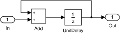
Figure 2: A Simulink diagram modeling the 1-step delayed sum of its input In. Each atomic block as well as the entire system can be formalized as STS components (see §3.2). The entire system can also be formalized as a composite component (see below).

As an example, consider the Simulink diagram shown in Fig. 2. This diagram can be represented in our language as a composite component $\mathtt{Sum}$ defined as

$$\mathtt{Sum}=\mathtt{fdbk}(\mathtt{Add}\,;\mathtt{UnitDelay}\,;\mathtt{Split})$$

where $\mathtt{Add}$, $\mathtt{UnitDelay}$, and $\mathtt{Split}$ are atomic components (for a definition of these atomic components see §3.2). Here $\mathtt{Split}$ models the “fan-out” element in the Simulink diagram (black bullet) where the output wire of $\mathtt{UnitDelay}$ splits in two wires going to $\mathtt{Out}$ and back to $\mathtt{Add}$.

3.2 Symbolic Transition System Components

We introduce all four categories of STS components and at the same time provide syntactic mappings from specialized STS components to general STS components.

3.2.1 General STS Components

A general symbolic transition system component (general STS component) is a transition system described symbolically, with Boolean expressions over input, output, state, and next state variables defining the initial states and the transition relation. When we say “Boolean expression” (here and in the definitions that follow) we mean an expression of type $\mathbb{B}$, in some arbitrary logic, not necessarily restricted to propositional logic. For example, if $x$ is a variable of numerical type, then $x>0$ is a Boolean expression. In the definition that follows, $s^{\prime}$ denotes the primed, or next state variable, corresponding to the current state variable $s$. Both can be vectors of variables. For example, if $s=(s_{1},s_{2})$ then $s^{\prime}=(s_{1}^{\prime},s_{2}^{\prime})$. We assume that $s^{\prime}$ has the same type as $s$.

Definition 1 (STS component).

A (general) STS component is a tuple

$$\mathtt{sts}(x:\Sigma_{x},y:\Sigma_{y},s:\Sigma_{s},\mathit{init\_exp}:\mathbb{B},\mathit{trs\_exp}:\mathbb{B})$$

where $x,y,s$ are input, output and state variables (or tuples of variables) of types $\Sigma_{x},\Sigma_{y},\Sigma_{s}$, respectively, $\mathit{init\_exp}$ is a Boolean expression on $s$ (in some logic), and $\mathit{trs\_exp}$ is a Boolean expression on $x,y,s,s^{\prime}$ (in some logic).

Intuitively, an STS component is a non-deterministic system which for an infinite input sequence $\sigma_{x}\in\Sigma_{x}^{\omega}$ produces as output an infinite sequence $\sigma_{y}\in\Sigma_{y}^{\omega}$. The system starts non-deterministically at some state $\sigma_{s}(0)$ satisfying $\mathit{init\_exp}$. Given first input $\sigma_{x}(0)$, the system non-deterministically computes output $\sigma_{y}(0)$ and next state $\sigma_{s}(1)$ such that $\mathit{trs\_exp}$ holds (if no such values exist, then the input $\sigma_{x}(0)$ is illegal, as discussed in more detail below). Next, it uses the following input $\sigma_{x}(1)$ and state $\sigma_{s}(1)$ to compute $\sigma_{y}(1)$ and $\sigma_{s}(2)$, and so on.

We will sometimes use the term contract to refer to the expression $\mathit{trs\_exp}$. Indeed, $\mathit{trs\_exp}$ can be seen as specifying a contract between the component and its environment, in the following sense. At each step in the computation, the environment must provide input values that do not immediately violate the contract, i.e., for which we can find values for the next state and output variables to satisfy $\mathit{trs\_exp}$. Then, it is the responsibility of the component to find such values, otherwise it is the component’s “fault” if the contract is violated. This game-theoretic interpretation is similar in spirit with the classic refinement calculus for sequential programs [10].

We use $\Sigma_{x}$, $\Sigma_{y}$, $\Sigma_{s}$ in the definition above to emphasize the types of the input, output and the state, and the fact that, when composing components, the types should match. However, in practice we often omit the types, unless they are required to unambiguously specify a component. Also note that the definition does not fix the logic used for the expressions $\mathit{init\_exp}$ and $\mathit{trs\_exp}$. Indeed, our theory and results are independent from the choice of this logic. The choice of logic matters for algorithmic complexity and decidability. We will return to this point in §5. Finally, for simplicity, we often view the formulas $\mathit{init\_exp}$ and $\mathit{trs\_exp}$ as semantic objects, namely, as predicates. Adopting this view, $\mathit{init\_exp}$ becomes the predicate $init:\Sigma_{s}\to\mathbb{B}$, and $\mathit{trs\_exp}$ the predicate $\mathit{trs\_exp}:\Sigma_{s}\to\Sigma_{x}\to\Sigma_{s}\to\Sigma_{y}\to\mathbb{B}$. Equivalently, $\mathit{trs\_exp}$ can be interpreted as a relation $\mathit{trs\_exp}:(\Sigma_{s}\times\Sigma_{x})\to(\Sigma_{s}\times\Sigma_{y})\to\mathbb{B}$.

Throughout this paper we assume that $\mathit{init\_exp}$ is satisfiable, meaning that there is at least one valid initial state.

Examples.

In the examples provided in this paper, we often specify systems that have tuples as input, state and output variables, in different equivalent ways. For example, we can introduce a general STS component with two inputs as $\mathtt{sts}((n:\mathbb{N},x:\mathbb{R}),s:\mathbb{R},y:\mathbb{R},s>0,s^{\prime}>s\land y+s=x^{n})$, but also as $\mathtt{sts}((n,x):\mathbb{N}\times\mathbb{R},s:\mathbb{R},y:\mathbb{R},s>0,s^{\prime}>s\land y+s=x^{n})$, or $\mathtt{sts}(z:\mathbb{N}\times\mathbb{R},y:\mathbb{R},s:\mathbb{R},s>0,s^{\prime}>s\land y+s=\mathsf{snd}(z)^{\mathsf{fst}(z)})$, where $\mathsf{fst}$ and $\mathsf{snd}$ return the first and second elements of a pair.

Let us model a system that at every step $i$ outputs the input received at previous step $i-1$ (assume that the initial output value is $0$). This corresponds to Simulink’s commonly used $\mathtt{UnitDelay}$ block, which is also modeled in the diagram of Fig. 2. This block can be represented by an STS component, where a state variable $s$ is needed to store the input at moment $i$ such that it can be used at the next step. We formally define this component as

$$\mathtt{UnitDelay}=\mathtt{sts}(x,y,s,s=0,y=s\land s^{\prime}=x).$$

We use first-order logic to define $\mathit{init\_exp}$ and $\mathit{trs\_exp}$. Here $\mathit{init\_exp}$ is $s=0$, which initializes the state variable $s$ with the value $0$. The $\mathit{trs\_exp}$ is $y=s\land s^{\prime}=x$, that is at moment $i$ the current state variable $s$ which stores the input $x$ received at moment $i-1$ is outputed and its value is updated.

As another example, consider again the composite component $\mathtt{Sum}$ modeling the diagram of Fig. 2. $\mathtt{Sum}$ could also be defined as an atomic STS component:

$$\mathtt{Sum}=\mathtt{sts}(x,y,s,s=0,y=s\land s^{\prime}=s+x).$$

In §5 we will show how we can automatically and symbolically simplify composite component terms such as $\mathtt{fdbk}(\mathtt{Add}\,;\mathtt{UnitDelay}\,;\mathtt{Split})$, to obtain syntactic representations of atomic components such as the one above.

These examples illustrate systems coming from Simulink models. However, our language is more general, and able to accommodate the description of other systems, such as state machines à la nuXmv [16], or input/output automata [54]. In fact, both $\mathtt{UnitDelay}$ and $\mathtt{Sum}$ are deterministic, so they could also be defined as deterministic STS components, as we will see below. Our language can capture non-deterministic systems easily. An example of a non-deterministic STS component is the following:

$$C=\mathtt{sts}(x,y,s,s=0,x+s\leq y).$$

For an input sequence $\sigma_{x}\in\mathbb{N}^{\omega}$, $C$ outputs a non-deterministically chosen sequence $\sigma_{y}$ such that the transition expression $x+s\leq y$ is satisfied. Since there is no formula in the transition expression tackling the next state variable, this is updated also non-deterministically with values from $\mathbb{N}$.

Our language can also capture non-input-receptive systems, that is, systems which disallow some input values as illegal. For instance, a component performing division, but disallowing division by zero, can be specified as follows:

$$\mathtt{Div}=\mathtt{sts}((x,y),z,(),\mathtt{true},y\neq 0\land z=\dfrac{x}{y}).$$

Note that $\mathtt{Div}$ has an empty tuple of state variables, $s=()$. Such components are called stateless, and are introduced in the sequel.

Even though RCRS is primarily a discrete-time framework, we have used it to model and verify continuous-time systems such as those modeled in Simulink (see §6). We do this by discretizing time using a time step parameter $\Delta t>0$ and applying Euler numerical integration. Then, we can model Simulink’s Integrator block in RCRS as an STS component parameterized by $\Delta t$:

$$\mathtt{Integrator}_{\Delta t} = \mathtt{sts}\big{(}x,y,s,s=0,y=s\land s^{\prime}=s+x\cdot\Delta t\big{)}$$

More complex dynamical system blocks can be modeled in a similar fashion. For instance, Simulink’s Transfer Fcn block, with transfer function

$$\frac{s^{2}+2}{0.5s^{2}+2s+1}$$

can be modeled in RCRS as the following STS component parameterized by $\Delta t$:

$$\mathtt{TransferFcn}_{\Delta t} = \mathtt{sts}\big{(}x,y,(s_{1},s_{2}),s_{1}=0\land s_{2}=0,trs)$$

$$\mbox{ where }\qquad trs = (y=-8\cdot s_{1}+2\cdot x)\ \land$$

$$\qquad(s_{1}^{\prime}=s_{1}+(-4\cdot s_{1}-2\cdot s_{2}+x)\cdot\Delta t)\ \land$$

$$\qquad(s_{2}^{\prime}=s_{2}+s_{1}\cdot\Delta t)$$

3.2.2 Variable Name Scope

We remark that variable names in the definition of atomic components are local. This holds for all atomic components in the language of RCRS (including STS and QLTL components, defined in the sequel). This means that if we replace a variable with another one in an atomic component, then we obtain a semantically equivalent component. For example, the two STS components below are equivalent (the semantical equivalence symbol $\equiv$ will be defined formally in Def. 20, once we define the semantics):

$$\mathtt{sts}((x,y),z,s,s>0,z>s+x+y)\equiv\mathtt{sts}((u,v),w,t,t>0,w>t+u+v)$$

3.2.3 Stateless STS Components

A special STS component is one that has no state variables:

Definition 2 (Stateless STS component).

A stateless STS component is a tuple

$$C=\mathtt{stateless}(x:\Sigma_{x},y:\Sigma_{y},\mathit{io\_exp}:\mathbb{B})$$

where $x,y$ are the input and output variables, and $\mathit{io\_exp}$ is a Boolean expression on $x$ and $y$. Stateless STS components are special cases of general STS components, as defined by the mapping $\mathtt{stateless}2\mathtt{sts}$:

$$\mathtt{stateless}2\mathtt{sts}(C)=\mathtt{sts}(x,y,(),\mathtt{true},\mathit{io\_exp}).$$

Examples.

A trivial stateless STS component is the one that simply transfers its input to its output (i.e., a “wire”). We denote such a component by $\mathtt{Id}$, and we formalize it as

$$\mathtt{Id}=\mathtt{stateless}(x,y,y=x).$$

Another simple example is a component with no inputs and a single output, which always outputs a constant value $c$ (of some type). This can be formalized as the following component parameterized by $c$:

$$\mathtt{Const}_{c}=\mathtt{stateless}((),y,y=c).$$

Component $\mathtt{Add}$ from Fig. 2, which outputs the sum of its two inputs, can be modeled as a stateless STS component:

$$\mathtt{Add}=\mathtt{stateless}((x,y),z,z=x+y).$$

Component $\mathtt{Split}$ from Fig. 2 can also be modeled as a stateless STS component:

$$\mathtt{Split}=\mathtt{stateless}(x,(y,z),y=x\land z=x).$$

The $\mathtt{Div}$ component introduced above is stateless, and therefore can be also specified as follows:

$$\mathtt{Div}=\mathtt{stateless}\big{(}(x,y),z,y\neq 0\land z=\dfrac{x}{y}\big{)}.$$

The above examples are not only stateless, but also deterministic. We introduce deterministic STS components next.

3.2.4 Deterministic STS Components

Deterministic STS components are those which, for given current state and input, have at most one output and next state. Syntactically, they are introduced as follows:

Definition 3 (Deterministic STS component).

A deterministic STS component is a tuple

$$\mathtt{det}(x:\Sigma_{x},s:\Sigma_{s},a:\Sigma_{s},\mathit{inpt\_exp}:\mathbb{B},\mathit{next\_exp}:\Sigma_{s},\mathit{out\_exp}:\Sigma_{y})$$

where $x,s$ are the input and state variables, $a\in\Sigma_{s}$ is the initial value of the state variable, $\mathit{inpt\_exp}$ is a Boolean expression on $s$ and $x$ defining the legal inputs, $\mathit{next\_exp}$ is an expression of type $\Sigma_{s}$ on $x$ and $s$ defining the next state, and $\mathit{out\_exp}$ is an expression of type $\Sigma_{y}$ on $x$ and $s$ defining the output. Deterministic STS components are special cases of general STS components, as defined by the mapping $\mathtt{det}2\mathtt{sts}$:

$$\mathtt{det}2\mathtt{sts}(C)=(x,y,s,s=a,\mathit{inpt\_exp}\land s^{\prime}=\mathit{next\_exp}\land y=\mathit{out\_exp})$$

where $y$ is a new variable name (or tuple of new variable names) of type $\Sigma_{y}$.

Note that a deterministic STS component has a separate expression $\mathit{inpt\_exp}$ to define legal inputs. A separate such expression is not needed for general STS components, where the conditions for legal inputs are part of the expression $\mathit{trs\_exp}$. For example, compare the definition of $\mathtt{Div}$ as a general STS above, and as a stateless deterministic STS below (see §3.2.5).

Examples.

As mentioned above, all three components, $\mathtt{UnitDelay}$, $\mathtt{Add}$, and $\mathtt{Split}$ from Fig. 2, as well as $\mathtt{Div}$ and $\mathtt{Const}$, are deterministic. They could therefore be specified in our language as deterministic STS components, instead of general STS components:

$$\mathtt{UnitDelay} = \mathtt{det}\big{(}x,s,0,\mathtt{true},x,s\big{)}$$

$$\mathtt{Const}_{c} = \mathtt{det}\big{(}(),(),(),\mathtt{true},(),c\big{)}$$

$$\mathtt{Add} = \mathtt{det}\big{(}(x,y),(),(),\mathtt{true},(),x+y\big{)}$$

$$\mathtt{Split} = \mathtt{det}\big{(}x,(),(),\mathtt{true},(),(x,x)\big{)}$$

$$\mathtt{Div} = \mathtt{det}\big{(}(x,y),(),(),y\not=0,(),\dfrac{x}{y}\big{)}$$

The component $\mathtt{Sum}$ modeling the entire system is also deterministic, and could be defined as a deterministic STS component:

$$\mathtt{Sum}=\mathtt{det}(x,s,0,\mathtt{true},s+x,s).$$

Note that these alternative specifications for each of those components, although syntactically distinct, will turn out to be semantically equivalent by definition, when we introduce the semantics of our language, in §4.

3.2.5 Stateless Deterministic STS Components

STS components which are both deterministic and stateless can be specified as follows:

Definition 4 (Stateless deterministic STS component).

A stateless deterministic STS component is a tuple

$$C=\mathtt{stateless\_det}(x:\Sigma_{x},\mathit{inpt\_exp}:\mathbb{B},\mathit{out\_exp}:\Sigma_{y})$$

where $x$ is the input variable, $\mathit{inpt\_exp}$ is a Boolean expression on $x$ defining the legal inputs, and $\mathit{out\_exp}$ is an expression of type $\Sigma_{y}$ on x defining the output. Stateless deterministic STS components are special cases of both deterministic STS components, and of stateless STS components, as defined by the mappings

$$\mathtt{stateless\_det}2\mathtt{det}(C) = \mathtt{det}(x,(),(),\mathit{inpt\_exp},(),\mathit{out\_exp})$$

$$\mathtt{stateless\_det}2\mathtt{stateless}(C) = \mathtt{stateless}(x,y,\mathit{inpt\_exp}\land y=\mathit{out\_exp})$$

where $y$ is a new variable name or a tuple of new variable names.

Examples.

Many of the examples introduced above are both deterministic and stateless. They could be specified as follows:

$$\begin{array}[]{lll}\mathtt{Id}&=&\mathtt{stateless\_det}\big{(}x,\mathtt{true},x\big{)}\\[4.30554pt] \mathtt{Const}_{c}&=&\mathtt{stateless\_det}\big{(}(),\mathtt{true},c\big{)}\\[4.30554pt] \mathtt{Add}&=&\mathtt{stateless\_det}\big{(}(x,y),\mathtt{true},x+y\big{)}\\[4.30554pt] \mathtt{Split}&=&\mathtt{stateless\_det}\big{(}x,\mathtt{true},(x,x)\big{)}\\[4.30554pt] \mathtt{Div}&=&\mathtt{stateless\_det}\big{(}(x,y),y\not=0,\dfrac{x}{y}\big{)}\end{array}$$

3.3 Quantified Linear Temporal Logic Components

Although powerful, STS components have limitations. In particular, they cannot express liveness properties [4]. To remedy this, we introduce another type of components, based on Linear Temporal Logic (LTL) [63] and quantified propositional LTL (QPTL) [76, 48], which extends LTL with $\exists$ and $\forall$ quantifiers over propositional variables. In this paper we use quantified first-order LTL (which we abbreviate as QLTL). QLTL further extends QPTL with functional and relational symbols over arbitrary domains, quantification of variables over these domains, and a next operator applied to variables. We need this expressive power in order to be able to handle general models (e.g., Simulink) which often use complex arithmetic formulas, and also to be able to translate STS components into semantically equivalent QLTL components (see §5.1).

3.3.1 QLTL

QLTL formulas are generated by the following grammar. We assume a set of constants and functional symbols ($0,1,\ldots$, $\mathtt{true},\mathtt{false}$, $+,\ldots$), a set of predicate symbols ($=,\leq,<,\ldots$), and a set of variable names ($x,y,z,\ldots$).

Definition 5 (Syntax of QLTL).

A QLTL formula $\varphi$ is defined by the following grammar:

$$\begin{array}[]{llll}term&::=&x\ |\ y\ |\ \ldots\ |&\text{(variable names)}\\ &&0\ |\ 1\ |\ \ldots\ |\ \mathtt{true}\ |\ \ldots\ |&\text{(constants)}\\ &&term+term\ |\ \ldots\ |&\text{(functional symbol application)}\\ &&\ocircle\,term&\text{(next applied to a term)}\\ \varphi&::=&term=term\ |\ (term\leq term)\ |\ \ldots\ |&\text{(atomic QLTL formulas)}\\ &&\neg\varphi\ |&\text{(negation)}\\ &&\varphi\lor\psi\ |&\text{(disjunction)}\\ &&\varphi\mathbf{\leavevmode\nobreak\ U\leavevmode\nobreak\ }\psi\ |&\text{(until)}\\ &&\forall x:\varphi&\text{(forall)}\end{array}$$

As in standard first order logic, the bounded variables of a formula $\varphi$ are the variables in scope of the universal quantifier $\forall$, and the free variables of $\varphi$ are those that are not bounded. The logic connectives $\land$, $\Rightarrow$ and $\Leftrightarrow$ can be expressed with $\neg$ and $\lor$. Quantification is over atomic variables. The existential quantifier $\exists$ can be defined via the universal quantifier usually as $\neg\forall\neg$. The primitive temporal operators are next for terms ($\ocircle\,$) and until ($\mathbf{\leavevmode\nobreak\ U\leavevmode\nobreak\ }$). As is standard, QLTL formulas are evaluated over infinite traces, and $\varphi\mathbf{\leavevmode\nobreak\ U\leavevmode\nobreak\ }\psi$ intuitively means that $\varphi$ continuously holds until some point in the trace where $\psi$ holds.

Formally, we will define the relation $\sigma\models\varphi$ ($\sigma$ satisfies $\varphi$) for a QLTL formula $\varphi$ over free variables $x,y,\ldots$, and an infinite sequence $\sigma\in\Sigma^{\omega}$, where $\Sigma=\Sigma_{x}\times\Sigma_{y}\times\ldots$, and $\Sigma_{x},\Sigma_{y},\ldots$ are the types (or domains) of variables $x,y,\ldots$. As before we assume that $\sigma$ can be written as a tuple of sequences $(\sigma_{x},\sigma_{y},\ldots)$ where $\sigma_{x}\in\Sigma_{x}^{\omega},\sigma_{y}\in\Sigma_{y}^{\omega},\ldots$. The semantics of a term $t$ on variables $x,y,\ldots$ is a function from infinite sequences to infinite sequences $\langle\!\langle t\rangle\!\rangle:\Sigma^{\omega}\to\Sigma_{t}^{\omega}$, where $\Sigma=\Sigma_{x}\times\Sigma_{y}\times\ldots$, and $\Sigma_{t}$ is the type of $t$. When giving the semantics of terms and formulas we assume that constants, functional symbols, and predicate symbols have the standard semantics. For example, we assume that $+,\leq,\ldots$ on numeric values have the semantics of standard arithmetic.

Definition 6 (Semantics of QLTL).

Let $x$ be a variable, $t,t^{\prime}$ be terms, $\varphi,\psi$ be QLTL formulas, $P$ be a predicate symbol, $f$ be a functional symbol, $c$ be a constant, and $\sigma\in\Sigma^{\omega}$ be an infinite sequence.

$$\begin{array}[]{lll}\langle\!\langle x\rangle\!\rangle(\sigma)&:=&\sigma_{x}\\ \langle\!\langle c\rangle\!\rangle(\sigma)&:=&(\lambda i:c)\\ \langle\!\langle f(t,t^{\prime})\rangle\!\rangle(\sigma)&:=&(\lambda i:f(\langle\!\langle t\rangle\!\rangle(\sigma)(i),\langle\!\langle t^{\prime}\rangle\!\rangle(\sigma)(i)))\\ \langle\!\langle\ocircle\,t\rangle\!\rangle(\sigma)&:=&\langle\!\langle t\rangle\!\rangle(\sigma^{1})\\[4.30554pt] \sigma\models P(t,t^{\prime})&:=&P(\langle\!\langle t\rangle\!\rangle(\sigma)(0),\langle\!\langle t^{\prime}\rangle\!\rangle(\sigma)(0))\\ \sigma\models\neg\varphi&:=&\neg\ \sigma\models\varphi\\ \sigma\models\varphi\lor\psi&:=&\sigma\models\varphi\lor\sigma\models\psi\\ \sigma\models\varphi\mathbf{\leavevmode\nobreak\ U\leavevmode\nobreak\ }\psi&:=&(\exists n\geq 0:(\forall\ 0\leq i<n:\sigma^{i}\models\varphi)\land\sigma^{n}\models\psi)\\ \sigma\models(\forall x:\varphi)&:=&(\forall\sigma_{x}\in\Sigma_{x}^{\omega}:(\sigma_{x},\sigma)\models\varphi)\par\end{array}$$

Other temporal operators can be defined as follows. Eventually ($\mathbf{F\,}\varphi=\mathtt{true}\mathbf{\leavevmode\nobreak\ U\leavevmode\nobreak\ }\varphi$) states that $\varphi$ must hold in some future step. Always ($\mathbf{G\,}\varphi=\neg\mathbf{F\,}\neg\varphi$) states that $\varphi$ must hold at all steps. The next operator for formulas $\mathbf{X\,}$ can be defined using the next operator for terms $\ocircle\,$. The formula $\mathbf{X\,}\varphi$ is obtained by replacing all occurrences of the free variables in $\varphi$ by their next versions (i.e., $x$ is replaced by $\ocircle\,x$, $y$ by $\ocircle\,y$, etc.). For example the propositional LTL formula $\mathbf{X\,}(x\land\mathbf{X\,}y\Rightarrow\mathbf{G\,}z)$ can be expressed as

$$(\ocircle\,x=\mathtt{true}\land(\ocircle\,\ocircle\,y=\mathtt{true})\Rightarrow\mathbf{G\,}(\ocircle\,z=\mathtt{true})).$$

We additionally introduce the operator: $\varphi\mathbf{\,L\,}\psi:=\neg(\varphi\mathbf{\leavevmode\nobreak\ U\leavevmode\nobreak\ }\neg\psi)$. Intuitively, $\varphi\mathbf{\,L\,}\psi$ holds if whenever $\varphi$ holds continuously up to some step $n-1$, $\psi$ must hold at step $n$.

Two QLTL formulas $\varphi$ and $\psi$ are semantically equivalent, denoted $\varphi\iff\psi$, if

$$\forall\sigma:(\sigma\models\varphi)\iff(\sigma\models\psi).$$

Lemma 1.

Let $\varphi$ be a QLTL formula. Then:

1. $(\exists x:\mathbf{G\,}\varphi)\iff\mathbf{G\,}(\exists x:\varphi)$ when $\varphi$ does not contain temporal operators.

2. $\varphi\mathbf{\,L\,}\varphi\iff\mathbf{G\,}\varphi$

3. $\mathtt{true}\mathbf{\,L\,}\varphi\iff\mathbf{G\,}\varphi$

4. $\varphi\mathbf{\,L\,}\mathtt{true}\iff\mathtt{true}$

5. $\varphi\mathbf{\,L\,}\mathtt{false}\iff\mathtt{false}$

6. $\forall y:(\varphi\mathbf{\,L\,}\psi)\iff(\exists y:\varphi)\mathbf{\,L\,}\psi$, when $\varphi$ does not contain temporal operators and $y$ is not free in $\psi$.

The proof of the above result, as well as of most results that follow, is omitted. All omitted proofs have been formalized and proved in the Isabelle proof assistant, and are available as part of the public distribution of RCRS from http://rcrs.cs.aalto.fi. In particular, all results contained in this paper can be accessed from the theory RCRS_Overview.thy – either directly in that file or via references to the other RCRS files.

Examples.

Using QLTL we can express safety, as well as liveness requirements. Informally, a safety requirement expresses that something bad never happens. An example is the formula

$$\mathtt{thermostat}=\mathbf{G\,}(180^{\circ}\leq t\land t\leq 220^{\circ}),$$

which states that the thermostat-controlled temperature $t$ stays always between $180^{\circ}$ and $220^{\circ}$.

A liveness requirement informally says that something good eventually happens. An example is the formula $\mathbf{F\,}(t>200^{\circ})$ stating that the temperature $t$ is eventually over $200^{\circ}$.

A more complex example is a formula modeling an oven that starts increasing the temperature from an initial value of $20^{\circ}$ until it reaches $180^{\circ}$, and then keeps it between $180^{\circ}$ and $220^{\circ}$.

$$\mathtt{oven}=(t=20^{\circ}\land((t<\ocircle\,t\land t<180)\mathbf{\leavevmode\nobreak\ U\leavevmode\nobreak\ }\mathtt{thermostat})).$$

In this example the formula $t<\ocircle\,t$ specifies that the temperature increases from some point to the next.

3.3.2 QLTL Components

A QLTL component is an atomic component where the input-output behavior is specified by a QLTL formula:

Definition 7 (QLTL component).

A QLTL component is a tuple $\mathtt{qltl}(x:\Sigma_{x},y:\Sigma_{y},\varphi)$, where $x,y$ are input and output variables (or tuples of variables) of types $\Sigma_{x},\Sigma_{y}$, and $\varphi$ is a QLTL formula over $x$ and $y$.

Intuitively a QLTL component $C=\mathtt{qltl}(x,y,\varphi)$ represents a system that takes as input an infinite sequence $\sigma_{x}\in\Sigma_{x}^{\omega}$ and produces as output an infinite sequence $\sigma_{y}\in\Sigma_{y}^{\omega}$ such that $(\sigma_{x},\sigma_{y})\models\varphi$. If there is no $\sigma_{y}$ such that $(\sigma_{x},\sigma_{y})\models\varphi$ is true, then input $\sigma_{x}$ is illegal for $C$, i.e., $C$ is not input-receptive. There could be many possible $\sigma_{y}$ for a single $\sigma_{x}$, in which case the system is non-deterministic.

As a simple example, we can model the oven as a QLTL component with no input variables and the temperature as the only output variable:

$$\mathtt{qltl}((),t,\mathtt{oven})$$

3.4 Well Formed Composite Components

Not all composite components generated by the grammar introduced in §3.1 are well formed. Two components $C$ and $C^{\prime}$ can be composed in series only if the number of outputs of $C$ matches the number of inputs of $C^{\prime}$, and in addition the input types of $C^{\prime}$ are the same as the corresponding output types of $C$. Also, $\mathtt{fdbk}$ can be applied to a component $C$ if the type of the first output of $C$ is the same as the type of its first input. Formally, for every component $C$ we define below $\Sigma_{in}(C)$ - the input type of $C$, $\Sigma_{out}(C)$ - the output type of $C$, and $\mathbf{wf}(C)$ - the well-formedness of $C$, by induction on the structure of $C$:

$$\begin{array}[]{lll}\Sigma_{in}(\mathtt{sts}(x:\Sigma_{x},y:\Sigma_{y},s:\Sigma_{s},init,trs))&=&\Sigma_{x}\\ \Sigma_{in}(\mathtt{stateless}(x:\Sigma_{x},y:\Sigma_{y},trs))&=&\Sigma_{x}\\ \Sigma_{in}(\mathtt{det}(x:\Sigma_{x},s:\Sigma_{s},a,inpt,next,out:\Sigma_{y}))&=&\Sigma_{x}\\ \Sigma_{in}(\mathtt{stateless\_det}(x:\Sigma_{x},inpt,out:\Sigma_{y}))&=&\Sigma_{x}\\ \Sigma_{in}(\mathtt{qltl}(x:\Sigma_{x},y:\Sigma_{y},\varphi))&=&\Sigma_{x}\\ \Sigma_{in}(C\;\,;\;C^{\prime})&=&\Sigma_{in}(C)\\ \Sigma_{in}(C\parallel C^{\prime})&=&\Sigma_{in}(C)\times\Sigma_{in}(C^{\prime})\\ \Sigma_{in}(\mathtt{fdbk}(C))&=&X_{2}\times\cdots\times X_{n}\mbox{ provided }\Sigma_{in}(C)=X_{1}\times\cdots\times X_{n}\\ &&\text{ for some }\ n\geq 1\end{array}$$

$$\begin{array}[]{lll}\Sigma_{out}(\mathtt{sts}(x:\Sigma_{x},y:\Sigma_{y},s:\Sigma_{s},init,trs))&=&\Sigma_{y}\\ \Sigma_{out}(\mathtt{stateless}(x:\Sigma_{x},y:\Sigma_{y},trs))&=&\Sigma_{y}\\ \Sigma_{out}(\mathtt{det}(x:\Sigma_{x},s:\Sigma_{s},a,inpt,next,out:\Sigma_{y}))&=&\Sigma_{y}\\ \Sigma_{out}(\mathtt{stateless\_det}(x:\Sigma_{x},inpt,out:\Sigma_{y}))&=&\Sigma_{y}\\ \Sigma_{out}(\mathtt{qltl}(x:\Sigma_{x},y:\Sigma_{y},\varphi))&=&\Sigma_{y}\\ \Sigma_{out}(C\;\,;\;C^{\prime})&=&\Sigma_{out}(C^{\prime})\\ \Sigma_{out}(C\parallel C^{\prime})&=&\Sigma_{out}(C)\times\Sigma_{out}(C^{\prime})\\ \Sigma_{out}(\mathtt{fdbk}(C))&=&Y_{2}\times\cdots\times Y_{n}\mbox{ provided }\Sigma_{out}(C)=Y_{1}\times\cdots\times Y_{n}\\ &&\text{ for some }n\geq 1\end{array}$$

$$\begin{array}[]{lll}\mathbf{wf}(\mathtt{sts}(x,y,s,init,trs))&=&true\\ \mathbf{wf}(\mathtt{stateless}(x,y,trs))&=&true\\ \mathbf{wf}(\mathtt{det}(x,s,a,inpt,next,out))&=&true\\ \mathbf{wf}(\mathtt{stateless\_det}(x,inpt,out))&=&true\\ \mathbf{wf}(\mathtt{qltl}(x,y,\varphi))&=&true\\ \mathbf{wf}(C\;\,;\;C^{\prime})&=&\mathbf{wf}(C)\land\mathbf{wf}(C^{\prime})\land\Sigma_{out}(C)=\Sigma_{in}(C^{\prime})\\ \mathbf{wf}(C\parallel C^{\prime})&=&\mathbf{wf}(C)\land\mathbf{wf}(C^{\prime})\\ \mathbf{wf}(\mathtt{fdbk}(C))&=&\mathbf{wf}(C)\land\Sigma_{in}(C)=X\times X_{1}\cdots\times X_{n}\\ &&\land\;\Sigma_{out}(C)=X\times Y_{1}\cdots\times Y_{m},\text{ for some }n,m\geq 0.\end{array}$$

In the definition above, both $n$ and $m$ are natural numbers. If $n=0$ then $X_{1}\times\cdots\times X_{n}$ denotes the $\mathsf{Unit}$ type.

Note that atomic components are by definition well-formed. The composite components considered in the sequel are required to be well-formed too.

We note that the above well-formedness conditions are not restrictive. Components that do not have matching inputs and outputs can still be composed by adding appropriate switching components which reorder inputs, duplicate inputs, and so on. An example of such a component is the component $\mathtt{Split}$, introduced earlier. As another example, consider the diagram in Fig. 3:

Figure 3: Another block diagram.

This diagram can be expressed in our language as the composite component:

$$\begin{array}[]{l}A\,;\mathtt{Switch1}\,;(B\parallel\mathtt{Id})\,;\mathtt{Switch2}\,;(C\parallel\mathtt{Id})\end{array}$$

where

$$\mathtt{Switch1} = \mathtt{stateless\_det}((x,y),\mathtt{true},(x,y,x))$$

$$\mathtt{Switch2} = \mathtt{stateless\_det}((u,v,x),\mathtt{true},(u,x,v))$$

4 Semantics

In RCRS, the semantics of components is defined in terms of monotonic property transformers (MPTs). This is inspired by classical refinement calculus [10], where the semantics of sequential programs is defined in terms of monotonic predicate transformers [28]. Predicate transformers are functions that transform sets of post-states (states reached after the program executes) into sets of pre-states (states from which the program begins). Property transformers map sets of output traces (that a component produces) into sets of input traces (that a component consumes).

In this section we define MPTs formally, and introduce some basic operations on them, which are necessary for giving the semantics of components. The definitions of some of these operations (e.g., product and fusion) are simple extensions of the corresponding operations on predicate transformers [10, 9]. Other operations, in particular those related to feedback, are new (§4.1.3). The definition of component semantics is also new (§4.3).

4.1 Monotonic Property Transformers

A property transformer is a function $S:(\Sigma_{y}^{\omega}\to\mathbb{B})\to(\Sigma_{x}^{\omega}\to\mathbb{B})$, where $\Sigma_{x},\Sigma_{y}$ are input and output types of the component in question. Note that $x$ is the input and $y$ is the output. A property transformer has a weakest precondition interpretation: it is applied to a set of output traces $Q\subseteq\Sigma_{y}^{\omega}$, and returns a set of input traces $P\subseteq\Sigma_{x}^{\omega}$, such that all traces in $P$ are legal and, when fed to the component, are guaranteed to produce only traces in $Q$ as output.

Interpreting properties as sets, monotonicity of property transformers simply means that these functions are monotonic with respect to set inclusion. That is, $S$ is monotonic if for any two properties $q,q^{\prime}$, if $q\subseteq q^{\prime}$ then $S(q)\subseteq S(q^{\prime})$.

For an MPT $S$ we define its set of legal input traces as $\mathsf{legal}(S)=S(\top)$, where $\top$ is the greatest predicate extended to traces. Note that, because of monotonicity, and the fact that $q\subseteq\top$ holds for any property $q$, we have that $S(q)\subseteq\mathsf{legal}(S)$ for all $q$. This justifies the definition of $\mathsf{legal}(S)$ as a “maximal” set of input traces for which a system does not fail, assuming no restrictions on the post-condition. An MPT $S$ is said to be input-receptive if $\mathsf{legal}(S)=\top$.

4.1.1 Some Commonly Used MPTs

Definition 8 (Skip).

$\mathsf{Skip}$ is defined to be the MPT such that for all $q$, $\mathsf{Skip}(q)=q$.

$\mathsf{Skip}$ models the identity function, i.e., the system that accepts all input traces and simply transfers them unchanged to the output (this will become more clear when we express $\mathsf{Skip}$ in terms of assert or update transformers, below). Note that $\mathsf{Skip}$ is different from $\mathtt{Id}$, defined above, although the two are strongly related: $\mathtt{Id}$ is a component, i.e., a syntactic object, while $\mathsf{Skip}$ is an MPT, i.e., a semantic object. As we shall see in §4.3, the semantics of $\mathtt{Id}$ is defined as $\mathsf{Skip}$.

Definition 9 (Fail).

$\mathsf{Fail}$ is defined to be the MPT such that for all $q$, $\mathsf{Fail}(q)=\bot$.

Recall that $\bot$ is the predicate that returns $\mathsf{false}$ for any input. Thus, viewed as a set, $\bot$ is the empty set. Consequently, $\mathsf{Fail}$ can be seen to model a system which rejects all inputs, i.e., a system such that for any output property $q$, there are no input traces that can produce an output trace in $q$.

Definition 10 (Assert).

Let $p\in\Sigma^{\omega}\to\mathbb{B}$ be a property. The assert property transformer $\{p\}:(\Sigma^{\omega}\to\mathbb{B})\to(\Sigma^{\omega}\to\mathbb{B})$ is defined by

$$\{p\}(q)=p\land q.$$

The assert transformer $\{p\}$ can be seen as modeling a system which accepts all input traces that satisfy $p$, and rejects all others. For all the traces that it accepts, the system simply transfers them, i.e., it behaves as the identity function.

To express MPTs such as assert transformers syntactically, let us introduce some notation. First, we can use lambda notation for predicates, as in $\lambda(\sigma,\sigma^{\prime}):(\sigma=\sigma^{\prime})$ for some predicate $p:\Sigma^{\omega}\to\Sigma^{\omega}\to\mathbb{B}$ which returns $\mathsf{true}$ whenever it receives two equal traces. Then, instead of writing $\{\lambda(\sigma,\sigma^{\prime}):(\sigma=\sigma^{\prime})\}$ for the corresponding assert transformer $\{p\}$, we will use the slightly lighter notation $\{\sigma,\sigma^{\prime}\mid\sigma=\sigma^{\prime}\}$.

Definition 11 (Demonic update).

Let $r:\Sigma_{x}^{\omega}\to\Sigma_{y}^{\omega}\to\mathbb{B}$ be a relation. The demonic update property transformer $[r]:(\Sigma_{y}^{\omega}\to\mathbb{B})\to(\Sigma_{x}^{\omega}\to\mathbb{B})$ is defined by

$$[r](q)=\{\sigma\ |\ \forall\sigma^{\prime}:r(\sigma)(\sigma^{\prime})\Rightarrow\sigma^{\prime}\in q\}.$$

That is, $[r](q)$ contains all input traces $\sigma$ which are guaranteed to result into an output trace in $q$ when fed into the (generally non-deterministic) input-output relation $r$. The term “demonic update” comes from the refinement calculus literature [10].

Similarly to assert, we introduce a lightweight notation for the demonic update. If $r$ is an expression in $\sigma$ and $\sigma^{\prime}$, then $[\sigma\leadsto\sigma^{\prime}\mid r]=[\lambda(\sigma,\sigma^{\prime}):r]$. For example, $[\sigma_{x},\sigma_{y}\leadsto\sigma_{z}\ |\ \forall i:\sigma_{z}(i)=\sigma_{x}(i)+\sigma_{y}(i)]$ is the system which produces as output the sequence $\sigma_{z}=(\lambda i:\sigma_{x}(i)+\sigma_{y}(i))$, where $\sigma_{x}$ and $\sigma_{y}$ are the input sequences. If $e$ is an expression in $\sigma$, then $[\sigma\leadsto e]$ is defined to be $[\sigma\leadsto\sigma^{\prime}\ |\ \sigma^{\prime}=e]$, where $\sigma^{\prime}$ is a new variable different from $\sigma$ and which does not occur free in $e$. For example, $[\sigma\leadsto(\lambda i:\sigma(i)+1)]=[\sigma\leadsto\sigma^{\prime}\ |\ \sigma^{\prime}=(\lambda i:\sigma(i)+1)]$.

The following lemma states that $\mathsf{Skip}$ can be defined as an assert transformer, or as a demonic update transformer.

Lemma 2.

$\mathsf{Skip}=[\sigma\leadsto\sigma^{\prime}\ |\ \sigma=\sigma^{\prime}]=\{\top\}=\{\sigma\mid\mathsf{true}\}$.

In general $\mathsf{Skip}$, $\mathsf{Fail}$, and other property transformers are polymorphic with respect to their input and output types. In $\mathsf{Skip}$ the input and output types must be the same. $\mathsf{Fail}$, on the other hand, may have an input type and a different output type.

Definition 12 (Angelic update).

Let $r:\Sigma_{x}^{\omega}\to\Sigma_{y}^{\omega}\to\mathbb{B}$ be a relation. The angelic update property transformer $\{r\}:(\Sigma_{y}^{\omega}\to\mathbb{B})\to(\Sigma_{x}^{\omega}\to\mathbb{B})$ is defined by

$$\{r\}(q)=\{\sigma\ |\ \exists\sigma^{\prime}:r(\sigma)(\sigma^{\prime})\land\sigma^{\prime}\in q\}.$$

An input sequence $\sigma$ is in $\{r\}(q)$ if there exists an output sequence $\sigma^{\prime}$ such that $r(\sigma)(\sigma^{\prime})$ and $\sigma^{\prime}\in q$. Notice the duality between the angelic and demonic update transformers. Consider, for example, a relation $r=\{(\sigma,\sigma^{\prime}),(\sigma,\sigma^{\prime\prime})\}$. If $q=\{\sigma^{\prime},\sigma^{\prime\prime}\}$, then $\{r\}(q)=[r](q)=\{\sigma\}$. If $q=\{\sigma^{\prime}\}$ then $\{r\}(q)=\{\sigma\}$, while $[r](q)=\emptyset$.

We use a lightweight notation for the angelic update transformer, similar to the one for demonic update. If $r$ is an expression in $\sigma$ and $\sigma^{\prime}$, then $\{\sigma\leadsto\sigma^{\prime}\ |\ r\}=\{\lambda(\sigma,\sigma^{\prime}):r\}$.

Lemma 3.

Assert is a particular case of angelic update: $\{p\}=\{\sigma\leadsto\sigma^{\prime}\ |\ p(\sigma)\land\sigma=\sigma^{\prime}\}$.

4.1.2 Operators on MPTs: Function Composition, Product, and Fusion

As we shall see in §4.3, the semantics of composition operators in the language of components will be defined by the corresponding composition operators on MPTs. We now introduce the latter operators on MPTs. First, we begin by the operators that have been known in the literature, and are recalled here. In §4.1.3 we introduce some novel operators explicitly designed in order to handle feedback composition.

Serial composition of MPTs (and property transformers in general) is simply function composition. Let $S:(\Sigma^{\omega}_{y}\to\mathbb{B})\to(\Sigma^{\omega}_{x}\to\mathbb{B})$ and $T:(\Sigma^{\omega}_{z}\to\mathbb{B})\to(\Sigma^{\omega}_{y}\to\mathbb{B})$ be two property transformers. Then $S\circ T:(\Sigma^{\omega}_{z}\to\mathbb{B})\to(\Sigma^{\omega}_{x}\to\mathbb{B})$, is the function composition of $S$ and $T$, i.e., $\forall q:(S\circ T)(q)=S(T(q))$. Note that serial composition preserves monotonicity, so that if $S$ and $T$ are MPTs, then $S\circ T$ is also an MPT. Also note that $\mathsf{Skip}$ is the neutral element for serial composition, i.e., $S\circ\mathsf{Skip}=\mathsf{Skip}\circ S=S$.

To express parallel composition of components, we need a kind of Cartesian product operation on property transformers. We define such an operation below. Similar operations for predicate transformers have been proposed in [9].

Definition 13 (Product).

Let $S:(\Sigma^{\omega}_{y}\to\mathbb{B})\to(\Sigma^{\omega}_{x}\to\mathbb{B})$ and $T:(\Sigma^{\omega}_{v}\to\mathbb{B})\to(\Sigma^{\omega}_{u}\to\mathbb{B})$. The product of $S$ and $T$, denoted $S\otimes T:(\Sigma^{\omega}_{y}\times\Sigma^{\omega}_{v}\to\mathbb{B})\to(\Sigma^{\omega}_{x}\times\Sigma^{\omega}_{u}\to\mathbb{B})$, is given by

$$(S\otimes T)(q)=\{(\sigma,\sigma^{\prime})\ |\ \exists p:\Sigma^{\omega}_{y}\to\mathbb{B},p^{\prime}:\Sigma^{\omega}_{v}\to\mathbb{B}:p\times p^{\prime}\subseteq q\land\sigma\in S(p)\land\sigma^{\prime}\in T(p^{\prime})\}$$

where $(p\times p^{\prime})(\sigma_{y},\sigma_{v})=p(\sigma_{y})\land p^{\prime}(\sigma_{v})$.

Lemma 4.

For arbitrary $S$ and $T$, $S\otimes T$ is monotonic.

The neutral element for the product composition is the $\mathsf{Skip}$ MPT that has $\mathsf{Unit}$ as input and output type.

In order to define a feedback operation on MPTs, we first define two auxiliary operations: Fusion and IterateOmega. Fusion is an extension of a similar operator introduced previously for predicate transformers in [9]. IterateOmega is a novel operator introduced in the sequel.

Definition 14 (Fusion).

If $S=\{S_{i}\}_{i\in I}$, $S_{i}:(\Sigma^{\omega}_{y}\to\mathbb{B})\to(\Sigma^{\omega}_{x}\to\mathbb{B})$ is a collection of MPTs, then the fusion of $S$ is the MPT $\mathsf{Fusion}_{i\in I}(S_{i}):(\Sigma^{\omega}_{y}\to\mathbb{B})\to(\Sigma^{\omega}_{x}\to\mathbb{B})$ defined by

$$(\mathsf{Fusion}_{i\in I}(S_{i}))(q)=\{\sigma\ |\ \exists p:I\to\Sigma_{y}^{\omega}\to\mathbb{B}:\bigcap_{i}p_{i}\subseteq q\land\sigma\in\bigcap_{i}S_{i}(p_{i})\}$$

The $\mathsf{Fusion}$ operator satisfies the following property.

Lemma 5.

For $I\not=\emptyset$ we have

$$\mathsf{Fusion}_{i\in I}(\{p_{i}\}\circ[r_{i}])=\{\bigcap_{i\in I}p_{i}\}\circ[\bigcap_{i\in I}r_{i}].$$

4.1.3 Novel Operators Used in Semantical Definition of Feedback

The IterateOmega operator is defined as follows:

Definition 15 (IterateOmega).

$$\mathsf{IterateOmega}(S)=\mathsf{Fusion}_{n\in\mathbb{N}}(S^{n}\circ[\sigma\leadsto\sigma^{\prime}\ |\ \forall i:i+1<n\Rightarrow\sigma_{i}=\sigma^{\prime}_{i}])$$

The feedback operator consists of connecting the first output of an MPT $S$ with its first input. Formally, feedback is defined as follows.

Definition 16 (Feedback).

Let $S:(\Sigma_{u}\times\Sigma_{y}^{\omega}\to\mathbb{B})\to(\Sigma_{u}\times\Sigma_{x}^{\omega}\to\mathbb{B})$ be an MPT. The feedback operator on $S$, denoted $\mathsf{Feedback}(S)$, is given by the MPT

$$\begin{array}[]{lll}\mathsf{Feedback}(S)&=&\{\sigma_{x}\leadsto\sigma_{u},\sigma_{y},\sigma_{x}\}\\ &&\circ\ \mathsf{IterateOmega}([\sigma_{u},\sigma_{y},\sigma_{x}\leadsto\sigma_{u},\sigma_{x},\sigma_{x}]\circ(S\otimes\mathsf{Skip}))\\ &&\circ\ [\sigma_{u},\sigma_{y},\sigma_{x}\leadsto\sigma_{y}]\end{array}$$

Example.

As an example we show how to derive $\mathsf{Feedback}(S)$ for $S=[\sigma_{u},\sigma_{x}\leadsto 0\cdot\sigma_{x}+0\cdot\sigma_{u},0\cdot\sigma_{x}+0\cdot\sigma_{u}]$, where $\sigma+\sigma^{\prime}=(\lambda i:\sigma(i)+\sigma^{\prime}(i))$, and $0\cdot\sigma$ is 0 concatenated with $\sigma$. For now, we note that $S$ is the semantics of the composite component $\mathtt{Add}\,;\mathtt{UnitDelay}\,;\mathtt{Split}$, which corresponds to the inner part of the diagram of Fig. 2, before applying feedback. We will complete the formal definition of the the semantics of this diagram in §4.3. For now, we focus on deriving $\mathsf{Feedback}(S)$, in order to illustrate how the $\mathsf{Feedback}$ operator works.

Let

$$T=[\sigma_{u},\sigma_{y},\sigma_{x}\leadsto\sigma_{u},\sigma_{x},\sigma_{x}]\circ(S\otimes\mathsf{Skip})=[\sigma_{u},\sigma_{y},\sigma_{x}\leadsto 0\cdot\sigma_{x}+0\cdot\sigma_{u},0\cdot\sigma_{x}+0\cdot\sigma_{u},\sigma_{x}]$$

Then, we have

$$\begin{array}[]{lll}T\circ T&=&[\sigma_{u},\sigma_{y},\sigma_{x}\leadsto 0\cdot\sigma_{x}+0\cdot 0\cdot\sigma_{x}+0\cdot 0\cdot\sigma_{u},0\cdot\sigma_{x}+0\cdot 0\cdot\sigma_{x}+0\cdot 0\cdot\sigma_{u},\sigma_{x}]\\ \ldots\\ T^{n}&=&[\sigma_{u},\sigma_{y},\sigma_{x}\leadsto 0\cdot\sigma_{x}+\ldots+0^{n}\cdot\sigma_{x}+0^{n}\cdot\sigma_{u},0\cdot\sigma_{x}+\ldots+0^{n}\cdot\sigma_{x}+0^{n}\cdot\sigma_{u},\sigma_{x}]\end{array}$$

where $0^{n}$ is a finite sequence of $n$ $0$s. We also have

$$\begin{array}[]{ll}&T^{n}\circ[\sigma\leadsto\sigma^{\prime}\ |\ \forall i:i+1<n\Rightarrow\sigma_{i}=\sigma^{\prime}_{i}]\\ =\\ &[\sigma_{u},\sigma_{y},\sigma_{x}\leadsto\sigma\ |\ \forall i:i+1<n\Rightarrow\sigma(i)=(\Sigma_{j<i}\sigma_{x}(j),\Sigma_{j<i}\sigma_{x}(j),\sigma_{x}(i))]\end{array}$$

Then

$$\begin{array}[]{ll}&\mathsf{Feedback}(S)\\ =\\ &\{\sigma_{x}\leadsto\sigma_{u},\sigma_{y},\sigma_{x}\}\circ\mathsf{IterateOmega}(T)\circ\ [\sigma_{u},\sigma_{y},\sigma_{x}\leadsto\sigma_{y}]\\ =\\ &\{\sigma_{x}\leadsto\sigma_{u},\sigma_{y},\sigma_{x}\}\circ\mathsf{Fusion}_{n\in\mathbb{N}}(T^{n}\circ[\sigma\leadsto\sigma^{\prime}\ |\ \forall i:i+1<n\Rightarrow\sigma_{i}=\sigma^{\prime}_{i}])\circ\ [\sigma_{u},\sigma_{y},\sigma_{x}\leadsto\sigma_{y}]\\ =\\ &\{\sigma_{x}\leadsto\sigma_{u},\sigma_{y},\sigma_{x}\}\circ\ [\sigma_{u},\sigma_{y},\sigma_{x}\leadsto\sigma\ |\ \forall i:\sigma(i)=(\Sigma_{j<i}\sigma_{x}(j),\Sigma_{j<i}\sigma_{x}(j),\sigma_{x}(i))]\circ\ [\sigma_{u},\sigma_{y},\sigma_{x}\leadsto\sigma_{y}]\\ =\\ &[\sigma_{x}\leadsto\sigma_{y}\ |\ \forall i:\sigma_{y}(i)=\Sigma_{j<i}\sigma_{x}(j)]\end{array}$$

Finally we obtain

$$\mathsf{Feedback}(S)=[\sigma_{x}\leadsto\sigma_{y}\ |\ \forall i:\sigma_{y}(i)=\Sigma_{j<i}\sigma_{x}(j)]$$ (2)

This is the system that outputs the trace $(\lambda i:\Sigma_{j<i}\sigma_{x}(j))$ for input trace $\sigma_{x}$.

4.1.4 Refinement

A key element of RCRS, as of other compositional frameworks, is the notion of refinement, which enables substitutability and other important concepts of compositionality. Semantically, refinement is defined as follows:

Definition 17 (Refinement).

Let $S,T:(\Sigma_{y}^{\omega}\to\mathbb{B})\to(\Sigma_{x}^{\omega}\to\mathbb{B})$ be two MPTs. We say that $T$ refines $S$ (or that $S$ is refined by $T$), written $S\sqsubseteq T$, if and only if $\forall q:S(q)\subseteq T(q)$.

All operations introduced on MPTs preserve the refinement relation:

Theorem 1.

If $S,T,S^{\prime},T^{\prime}$ are MPTs of appropriate types such that $S\sqsubseteq S^{\prime}$ and $T\sqsubseteq T^{\prime}$, then

1. $S\circ T\sqsubseteq S^{\prime}\circ T^{\prime}$ and $S\otimes T\sqsubseteq S^{\prime}\otimes T^{\prime}$ and $\mathsf{Fusion}(S,T)\sqsubseteq\mathsf{Fusion}(S^{\prime},T^{\prime})$ ([9, 10])

2. $\mathsf{IterateOmega}(S)\sqsubseteq\mathsf{IterateOmega}(S^{\prime})$

3. $\mathsf{Feedback}(S)\sqsubseteq\mathsf{Feedback}(S^{\prime})$

4.2 Subclasses of MPTs

Monotonic property transformers are a very rich and powerful class of semantic objects. In practice, the systems that we deal with often fall into restricted subclasses of MPTs, which are easier to represent syntactically and manipulate symbolically. We introduce these subclasses next.

4.2.1 Relational MPTs

Definition 18 (Relational property transformers).

A relational property transformer (RPT) $S$ is an MPT of the form $\{p\}\circ[r]$. We call $p$ the precondition of $S$ and $r$ the input-output relation of $S$.

Relational property transformers correspond to conjunctive transformers [10]. A transformer $S$ is conjunctive if it satisfies $S(\bigcap_{i\in I}q_{i})=\bigcap_{i\in I}S(q_{i})$ for all $(q_{i})_{i\in I}$ and $I\not=\emptyset$.

$\mathsf{Fail}$, $\mathsf{Skip}$, any assert transformer $\{p\}$, and any demonic update transformer $[r]$, are RPTs. Indeed, $\mathsf{Fail}$ can be written as $\{\sigma\ |\ \mathtt{false}\}\circ[\sigma\leadsto\sigma^{\prime}\ |\ \mathtt{true}]$. $\mathsf{Skip}$ can be written as $\{\sigma\ |\ \mathtt{true}\}\circ[\sigma\leadsto\sigma]$. The assert transformer $\{p\}$ can be written as the RPT $\{p\}\circ[\sigma\leadsto\sigma]$. Finally, the demonic update transformer $[r]$ can be written as the RPT $\{\sigma\ |\ \mathtt{true}\}\circ[r]$. Angelic update transformers are generally not RPTs: the angelic update transformer $\{\sigma\leadsto\sigma^{\prime}\ |\ \mathtt{true}\}$ is not an RPT, as it is not conjunctive.

Examples.

Suppose we wish to specify a system that performs division. Here are two possible ways to represent this system with RPTs:

$$S_{1}=\{\top\}\circ[\sigma_{x},\sigma_{y}\leadsto\sigma_{z}\ |\ \forall i:\sigma_{y}(i)\not=0\land\sigma_{z}(i)=\frac{\sigma_{x}(i)}{\sigma_{y}(i)}]$$

$$S_{2}=\{\sigma_{x},\sigma_{y}\ |\ \forall i:\sigma_{y}(i)\not=0\}\circ[\sigma_{x},\sigma_{y}\leadsto\sigma_{z}\ |\ \sigma_{z}(i)=\frac{\sigma_{x}(i)}{\sigma_{y}(i)}]$$

Although $S_{1}$ and $S_{2}$ are both relational, they are not equivalent transformers. $S_{1}$ is input-receptive: it accepts all input traces. However, if at some step $i$ the input $\sigma_{y}(i)$ is $0$, then the output $\sigma_{z}(i)$ is arbitrary (non-deterministic). In contrast, $S_{2}$ is non-input-receptive as it accepts only those traces $\sigma_{y}$ that are guaranteed to be non-zero at every step, i.e., those that satisfy the condition $\forall i:\sigma_{y}(i)\not=0$.

Theorem 2 (RPTs are closed under serial, product and fusion compositions).

Let $S=\{p\}\circ[r]$ and $S^{\prime}=\{p^{\prime}\}\circ[r^{\prime}]$ be two RPTs, with $p$, $p^{\prime}$, $r$ and $r^{\prime}$ of appropriate types. Then

$$S\circ S^{\prime}=\{\sigma\ |\ p(\sigma)\land(\forall\sigma^{\prime}:r(\sigma)(\sigma^{\prime})\Rightarrow p^{\prime}(\sigma^{\prime}))\}\circ[r\circ r^{\prime}]$$

and

$$S\otimes S^{\prime}=\{\sigma_{x},\sigma_{y}\ |\ p(\sigma_{x})\land p^{\prime}(\sigma_{y})\}\circ[\sigma_{x},\sigma_{y}\leadsto\sigma_{x}^{\prime},\sigma_{y}^{\prime}\ |\ r(\sigma_{x})(\sigma_{x}^{\prime})\land r^{\prime}(\sigma_{y})(\sigma_{y}^{\prime})]$$

and

$$\mathsf{Fusion}(S,S^{\prime})=\{p\land p^{\prime}\}\circ[r\land r^{\prime}]$$

RPTs are not closed under $\mathsf{Feedback}$. For example, we have

$$\mathsf{Feedback}([\sigma_{x},\sigma_{z}\leadsto\sigma_{x},\sigma_{x}])=\{\sigma\leadsto\sigma^{\prime}\ |\ \mathtt{true}\}$$

which is a non-relational angelic update transformer as we said above.

Next theorem shows that the refinement of RPTs can be reduced to proving a first order property.

Theorem 3.

For $p,p^{\prime},r,r^{\prime}$ of appropriate types we have.

$$\{p\}\circ[r]\sqsubseteq\{p^{\prime}\}\circ[r^{\prime}]\iff(p\subseteq p^{\prime}\land(\forall\sigma_{x}:p(\sigma_{x})\Rightarrow r^{\prime}(\sigma_{x})\subseteq r(\sigma_{x})))$$

4.2.2 Guarded MPTs

Relational property transformers correspond to systems that have natural syntactic representations, as the composition $\{p\}\circ[r]$, where the predicate $p$ and the relation $r$ can be represented syntactically in some logic. Unfortunately, RPTs are still too powerful. In particular, they allow system semantics that cannot be implemented. For example, consider the RPT $\mathsf{Magic}=[\sigma\leadsto\sigma^{\prime}\ |\ \mathsf{false}]$. It can be shown that for any output property $q$ (including $\bot$), we have $\mathsf{Magic}(q)=\top$. Recall that, viewed as a set, $\top$ is the set of all traces. This means that, no matter what the post-condition $q$ is, $\mathsf{Magic}$ somehow manages to produce output traces satisfying $q$ no matter what the input trace is (hence the name “magic”). In general, an MPT $S$ is said to be non-miraculous (or to satisfy the law of excluded miracle) if $S(\bot)=\bot$. We note that in [28], sequential programs are modeled using predicate transformers that are conjunctive and satisfy the low of excluded miracle.

We want to further restrict RPTs so that miraculous behaviour does not arise. Specifically, for an RPT $S=\{p\}\circ[r]$ and an input sequence $\sigma$, if there is no $\sigma^{\prime}$ such that $r(\sigma)(\sigma^{\prime})$ is satisfied, then we want $\sigma$ to be illegal, i.e., we want $p(\sigma)=\mathsf{false}$. We can achieve this by taking $p$ to be $\mathsf{in}(r)$. Recall that if $r:X\to Y\to\mathbb{B}$, then $\mathsf{in}(r)(x)=(\exists y:r(x)(y))$. Taking $p$ to be $\mathsf{in}(r)$ effectively means that $p$ and $r$ are combined into a single specification $r$ which can also restrict the inputs. This is also the approach followed in the theory of relational interfaces [79].

Definition 19 (Guarded property transformers).

The guarded property transformer (GPT) of a relation $r$ is an RPT, denoted $\{r]$, defined by $\{r]=\{\mathsf{in}(r)\}\circ[r]$.

It can be shown that an MPT $S$ is a GPT if and only if $S$ is conjunctive and non-miraculous [10]. $\mathsf{Fail}$, $\mathsf{Skip}$, and any assert property transformer are GPTs. Indeed, $\mathsf{Fail}=\{\bot]$ and $\mathsf{Skip}=\{\sigma\leadsto\sigma\ |\ \top]$. The assert transformer can be written as $\{p\}=\{\sigma\leadsto\sigma\ |\ p(\sigma)]$. The angelic and demonic update property transformers are generally not GPTs. The angelic update property transformer is not always conjunctive in order to be a GPT. The demonic update property transformer is not in general a GPT because is not always non-miraculous ($\mathsf{Magic}(\bot)=\top\not=\bot$). The demonic update transformer $[r]$ is a GPT if and only if $\mathsf{in}(r)=\top$ and in this case we have $[r]=\{r]$.

Theorem 4 (GPTs are closed under serial and parallel compositions).

Let $S=\{r]$ and $S^{\prime}=\{r^{\prime}]$ be two GPTs with $r$ and $r^{\prime}$ of appropriate types. Then

$$S\circ S^{\prime}=\{\sigma_{x}\leadsto\sigma_{z}\ |\ \mathsf{in}(r)(\sigma_{x})\land\big{(}\forall\sigma_{y}:r(\sigma_{x})(\sigma_{y})\Rightarrow\mathsf{in}(r^{\prime})(\sigma_{y})\big{)}\land(r\circ r^{\prime})(\sigma_{x},\sigma_{z})]$$

and

$$S\otimes S^{\prime}=\{\sigma_{x},\sigma_{y}\leadsto\sigma^{\prime}_{x},\sigma^{\prime}_{y}\ |\ r(\sigma_{x})(\sigma^{\prime}_{x})\land r^{\prime}(\sigma_{y})(\sigma^{\prime}_{y})]$$

GPTs are not closed under $\mathsf{Fusion}$ neither $\mathsf{Feedback}$. Indeed, we have already seen in the previous section that $\mathsf{Feedback}$ applied to the GPT $[\sigma_{x},\sigma_{z}\leadsto\sigma_{x},\sigma_{x}]$ is not an RPT, and therefore not a GPT either. For the fusion operator, we have $\mathsf{Fusion}([x\leadsto 0],[x\leadsto 1])=[\bot]$, which is not a GPT.

A corollary of Theorem 3 is that refinement of GPTs can be checked as follows:

Corollary 1.

$$\{r]\sqsubseteq\{r^{\prime}]\iff(\mathsf{in}(r)\subseteq\mathsf{in}(r^{\prime})\land(\forall\sigma_{x}:\mathsf{in}(r)(\sigma_{x})\Rightarrow r^{\prime}(\sigma_{x})\subseteq r(\sigma_{x})))$$

4.2.3 Other subclasses and overview

The containment relationships among the various subclasses of MPTs are illustrated in Fig. 4. In addition to the subclasses discussed above, we introduce several more subclasses of MPTs in the sections that follow, when we assign semantics (in terms of MPTs) to the various atomic components in our component language. For instance, QLTL components give rise to QLTL property transformers. Similarly, STS components, stateless STS components, etc., give rise to corresponding subclasses of MPTs. The containment relationships between these classes will be proven in the sections that follow. For ease of reference, we provide some forward links to these results also here. The fact that QLTL property transformers are GPTs follows by definition of the semantics of QLTL components: see §4.3, equation (3). The fact that STS property transformers are a special case of QLTL property transformers follows from the transformation of an STS component into a semantically equivalent QLTL component: see §5.1 and Theorem 7. The inclusions for subclasses of STS property transformers follow by definition of the corresponding components (see also Fig. 5).

Figure 4: Overview of the property transformer classes and their containment relations.

4.3 Semantics of Components as MPTs

We are now ready to define the semantics of our language of components in terms of MPTs. Let $C$ be a well formed component. The semantics of $C$, denoted $[\![C]\!]$, is a property transformer of the form:

$$[\![C]\!]:((\Sigma_{out}(C))^{\omega}\to\mathbb{B})\to((\Sigma_{in}(C))^{\omega}\to\mathbb{B}).$$

We define $[\![C]\!]$ by induction on the structure of $C$. First we give the semantics of QLTL components and composite components:

$$[\![\mathtt{qltl}(x,y,\varphi)]\!] = \{\sigma_{x}\leadsto\sigma_{y}\ |\ (\sigma_{x},\sigma_{y})\models\varphi]$$ (3)

$$[\![C\,;C^{\prime}]\!] = [\![C]\!]\circ[\![C^{\prime}]\!]$$ (4)

$$[\![C\parallel C^{\prime}]\!] = [\![C]\!]\otimes[\![C^{\prime}]\!]$$ (5)

$$[\![\mathtt{fdbk}(C)]\!] = \mathsf{Feedback}([\![C]\!])$$ (6)

The semantics of QLTL components satisfies the following property:

Lemma 6.

If $\varphi$ is a LTL formula on variables $x$ and $y$, we have:

$$[\![\mathtt{qltl}(x,y,(\exists y:\varphi)\land\varphi)]\!]=[\![\mathtt{qltl}(x,y,\varphi)]\!]$$

To define the semantics of STS components, we first introduce some auxiliary notation.

Consider an STS component $C=\mathtt{sts}(x,y,s,\mathit{init\_exp},\mathit{trs\_exp})$. We define the predicate $\mathsf{run}_{C}:\Sigma_{s}^{\omega}\times\Sigma_{x}^{\omega}\times\Sigma_{y}^{\omega}\to\mathbb{B}$ as

$$\mathsf{run}_{C}(\sigma_{s},\sigma_{x},\sigma_{y})=(\forall i:\mathit{trs\_exp}(\sigma_{s}(i),\sigma_{x}(i))(\sigma_{s}(i+1),\sigma_{y}(i))).$$

Intuitively, if $\sigma_{x}\in\Sigma_{x}^{\omega}$ is the input sequence, $\sigma_{y}\in\Sigma_{y}^{\omega}$ is the output sequence, and $\sigma_{s}\in\Sigma_{s}^{\omega}$ is the sequence of values of state variables, then $\mathsf{run}_{C}(\sigma_{s},\sigma_{x},\sigma_{y})$ holds if at each step of the execution, the current state, current input, next state, and current output, satisfy the $\mathit{trs\_exp}$ predicate.

We also formalize the illegal input traces of STS component $C$ as follows:

$$\mathsf{illegal}_{C}(\sigma_{x})=(\exists\sigma_{s},\sigma_{y},k:\mathit{init\_exp}(\sigma_{s}(0))\ \land(\forall i<k:\mathit{trs\_exp}(\sigma_{s}(i),\sigma_{x}(i))(\sigma_{s}(i+1),\sigma_{y}(i)))\ \land$$

$$\neg\mathsf{in}(\mathit{trs\_exp})(\sigma_{s}(k),\sigma_{x}(k)))$$

Essentially, $\mathsf{illegal}_{C}(\sigma_{x})$ states that there exists some point in the execution where the current state and current input violate the precondition $\mathsf{in}(\mathit{trs\_exp})$ of predicate $\mathit{trs\_exp}$, i.e., there exist no output and next state to satisfy $\mathit{trs\_exp}$ for that given current state and input.

Then, the semantics of an STS component $C$ is given by:

$$[\![C]\!]=\{\neg\mathsf{illegal}_{C}\}\circ[\sigma_{x}\leadsto\sigma_{y}\ |\ (\exists\sigma_{s}:\mathit{init\_exp}(\sigma_{s}(0))\land\mathsf{run}_{C}(\sigma_{s},\sigma_{x},\sigma_{y}))]$$ (7)

We give semantics to stateless and/or deterministic STS components using the corresponding mappings from general STS components. If $C$ is a stateless STS, $C^{\prime}$ is a deterministic STS, and $C^{\prime\prime}$ is a stateless deterministic STS, then:

$$[\![C]\!] = [\![\mathtt{stateless}2\mathtt{sts}(C)]\!]$$ (8)

$$[\![C^{\prime}]\!] = [\![\mathtt{det}2\mathtt{sts}(C^{\prime})]\!]$$ (9)

$$[\![C^{\prime\prime}]\!] = [\![\mathtt{stateless\_det}2\mathtt{det}(C^{\prime\prime})]\!]$$ (10)

Note that the semantics of a stateless deterministic STS component $C^{\prime\prime}$ is defined by converting $C^{\prime\prime}$ into a deterministic STS component, by Equation (10) above. Alternatively, we could have defined the semantics of $C^{\prime\prime}$ by converting it into a stateless STS component, using the mapping $\mathtt{stateless\_det}2\mathtt{stateless}$. In order for our semantics to be well-defined, we need to show that regardless of which conversion we choose, we obtain the same result. Indeed, this is shown by the lemma that follows:

Lemma 7.

For a stateless deterministic STS $C^{\prime\prime}$ we have:

$$[\![\mathtt{stateless\_det}2\mathtt{det}(C^{\prime\prime})]\!]=[\![\mathtt{stateless\_det}2\mathtt{stateless}(C^{\prime\prime})]\!]$$ (11)

Observe that, by definition, the semantics of QLTL components are GPTs. The semantics of STS components are defined as RPTs. However, they will be shown to be GPTs in §5.1. Therefore, the semantics of all atomic RCRS components are GPTs. This fact, and the closure of GPTs w.r.t. parallel and serial composition (Theorem 4), ensure that we stay within the GPT realm as long as no feedback operations are used. In addition, as we shall prove in Corollary 2, components with feedback are also GPTs, as long as they are deterministic and do not contain algebraic loops. An example of a component whose semantics is not a GPT is:

$$C=\mathtt{fdbk}(\mathtt{stateless}((x,z),(y_{1},y_{2}),y_{1}=x\land y_{2}=x))$$

Then, we have $[\![C]\!]=\mathsf{Feedback}([\sigma_{x},\sigma_{z}\leadsto\sigma_{x},\sigma_{x}])$. As stated earlier, $\mathsf{Feedback}([\sigma_{x},\sigma_{z}\leadsto\sigma_{x},\sigma_{x}])$ is equal to $\{\sigma\leadsto\sigma^{\prime}\ |\ \mathtt{true}\}$, which is not a GPT neither an RPT. The problem with $C$ is that it contains an algebraic loop: the first output $y_{1}$ of the internal stateless component where feedback is applied directly depends on its first input $x$. Dealing with such components is beyond the scope of this paper, and we refer the reader to [67].

4.3.1 Example: Two Alternative Derivations of the Semantics of Diagram $\mathtt{Sum}$ of Fig. 2

To illustrate our semantics, we provide two alternative derivations of the semantics of the $\mathtt{Sum}$ system of Fig. 2.

First, let us consider $\mathtt{Sum}$ as a composite component:

$$\mathtt{Sum}=\mathtt{fdbk}(\mathtt{Add}\,;\mathtt{UnitDelay}\,;\mathtt{Split})$$

where

$$\begin{array}[]{lll}\mathtt{Add}&=&\mathtt{stateless\_det}((u,x),\mathtt{true},u+x)\\ \mathtt{UnitDelay}&=&\mathtt{det}(x,s,0,\mathtt{true},x,s)\\ \mathtt{Split}&=&\mathtt{stateless\_det}(x,\mathtt{true},(x,x))\\ \end{array}$$

We have

$$\begin{array}[]{lll}[\![\mathtt{Sum}]\!]&=&[\![\mathtt{fdbk}(\mathtt{Add}\,;\mathtt{UnitDelay}\,;\mathtt{Split})]\!]\\ &=&\mathsf{Feedback}([\![\mathtt{Add}]\!]\circ[\![\mathtt{UnitDelay}]\!]\circ[\![\mathtt{Split}]\!])\end{array}$$

For ${\mathtt{Add}}$, ${\mathtt{UnitDelay}}$ and ${\mathtt{Split}}$, all inputs are legal, so $\mathsf{illegal}_{C}=\bot$ for all $C\in\{\mathtt{Add},\mathtt{UnitDelay},\mathtt{Split}\}$. After simplifications, we get:

$$\begin{array}[]{lll}[\![\mathtt{Add}]\!]&=&[\sigma_{u},\sigma_{x}\leadsto\sigma_{u}+\sigma_{x}]\\ [\![\mathtt{UnitDelay}]\!]&=&[\sigma_{x}\leadsto 0\cdot\sigma_{x}]\\ [\![\mathtt{Split}]\!]&=&[\sigma_{x}\leadsto\sigma_{x},\sigma_{x}]\end{array}$$

The semantics of $\mathtt{Sum}$ is given by

$$\begin{array}[]{lll}&[\![\mathtt{Sum}]\!]\\ =\\ &\mathsf{Feedback}([\![\mathtt{Add}]\!]\circ[\![\mathtt{UnitDelay}]\!]\circ[\![\mathtt{Split}]\!]\\ =\\ &\mathsf{Feedback}([\sigma_{u},\sigma_{x}\leadsto\sigma_{u}+\sigma_{x}]\circ[\sigma_{x}\leadsto 0\cdot\sigma_{x}]\circ[\sigma_{x}\leadsto\sigma_{x},\sigma_{x}])\\ =\\ &\mathsf{Feedback}([\sigma_{u},\sigma_{x}\leadsto 0\cdot\sigma_{x}+0\cdot\sigma_{u},0\cdot\sigma_{x}+0\cdot\sigma_{u}])\\[4.30554pt] =&\{\mbox{Using (\ref{eq:ex-feedback}})\}\\[4.30554pt] &[\sigma_{x}\leadsto\sigma_{y}\ |\ \forall i:\sigma_{y}(i)=\Sigma_{j<i}\sigma_{x}(j)]\par\end{array}$$

We obtain:

$$[\![\mathtt{Sum}]\!]=[\sigma_{x}\leadsto\sigma_{y}\ |\ \forall i:\sigma_{y}(i)=\Sigma_{j<i}\sigma_{x}(j)].$$ (12)

Next, let us assume that the system has been characterized already as an atomic component:

$$\mathtt{SumAtomic}=\mathtt{sts}(x,y,s,s=0,y=s\land s^{\prime}=s+x).$$

The semantics of $\mathtt{SumAtomic}$ is given by

$$[\![\mathtt{SumAtomic}]\!]=\{\neg\mathsf{illegal}_{\mathtt{SumAtomic}}\}\circ[\sigma_{x}\leadsto\sigma_{y}\ |\ \exists\sigma_{s}:\sigma_{s}(0)=0\land\mathsf{run}_{\mathtt{SumAtomic}}(\sigma_{s},\sigma_{x},\sigma_{y})]$$

where $\mathsf{illegal}_{\mathtt{SumAtomic}}=\bot$ because there are no restrictions on the inputs of $\mathtt{SumAtomic}$, and

$$\mathsf{run}_{\mathtt{SumAtomic}}(\sigma_{s},\sigma_{x},\sigma_{y})=\big{(}\forall i:\sigma_{y}(i)=\sigma_{s}(i)\land\sigma_{s}(i+1)=\sigma_{s}(i)+\sigma_{x}(i)\big{)}$$

We have

$$[\![\mathtt{SumAtomic}]\!]=[\sigma_{x}\leadsto\sigma_{y}\ |\ \exists\sigma_{s}:\sigma_{s}(0)=0\land\big{(}\forall i:\sigma_{y}(i)=\sigma_{s}(i)\land\sigma_{s}(i+1)=\sigma_{s}(i)+\sigma_{x}(i)\big{)}]$$

which is equivalent to (12).

4.3.2 Characterization of Legal Input Traces

The following lemma characterizes legal input traces for various types of MPTs:

Lemma 8.

The set of legal input traces of an RPT $\{p\}\circ[r]$ is $p$:

$$\mathsf{legal}(\{p\}\circ[r])=p.$$

The set of legal input traces of a GPT $\{r]$ is $\mathsf{in}(r)$:

$$\mathsf{legal}(\{r])=\mathsf{in}(r).$$

The set of legal input traces of an STS component $C=\mathtt{sts}(x,y,s,init,r)$ is equal to $\neg\mathsf{illegal}_{C}$:

$$\mathsf{legal}([\![C]\!])=\neg\mathsf{illegal}_{C}.$$

The set of legal input traces of a QLTL component $C=\mathtt{qltl}(x,y,\varphi)$ is:

$$\mathsf{legal}([\![C]\!])=\{\sigma_{x}\mid\sigma_{x}\models\exists y:\varphi\}.$$

4.3.3 Semantic Equivalence and Refinement for Components

Definition 20.

Two components $C$ and $C^{\prime}$ are (semantically) equivalent, denoted $C\equiv C^{\prime}$, if $[\![C]\!]=[\![C^{\prime}]\!]$. Component $C$ is refined by component $C^{\prime}$, denoted $C\preceq C^{\prime}$, if $[\![C]\!]\sqsubseteq[\![C^{\prime}]\!]$.

The relation $\equiv$ is an equivalence relation, and $\preceq$ is a preorder relation (i.e., reflexive and transitive). We also have

$$(C\preceq C^{\prime}\land C^{\prime}\preceq C)\iff(C\equiv C^{\prime})$$

4.3.4 Compositionality Properties

Several desirable compositionality properties follow from our semantics:

Theorem 5.

Let $C_{1}$, $C_{2}$, $C_{3}$, and $C_{4}$ be four (possibly composite) components. Then:

1. (Serial composition is associative:) $(C_{1}\,;C_{2})\,;C_{3}\equiv C_{1}\,;(C_{2}\,;C_{3})$.

2. (Parallel composition is associative:) $(C_{1}\parallel C_{2})\parallel C_{3}\equiv C_{1}\parallel(C_{2}\parallel C_{3})$.

3. (Parallel composition distributes over serial composition:) If $[\![C_{1}]\!]$ and $[\![C_{2}]\!]$ are GPTs and $[\![C_{3}]\!]$ and $[\![C_{4}]\!]$ are RPTs, then $(C_{1}\parallel C_{2})\,;(C_{3}\parallel C_{4})\equiv(C_{1}\,;C_{3})\parallel(C_{2}\,;C_{4})$.

4. (Refinement is preserved by composition:) If $C_{1}\preceq C_{2}$ and $C_{3}\preceq C_{4}$, then:

   1. $C_{1}\,;C_{3}\preceq C_{2}\,;C_{4}$

   2. $C_{1}\parallel C_{3}\preceq C_{2}\parallel C_{4}$

   3. $\mathtt{fdbk}(C_{1})\preceq\mathtt{fdbk}(C_{2})$

In addition to the above, requirements that a component satisfies are preserved by refinement. Informally, if $C$ satisfies some requirement $\varphi$ and $C\preceq C^{\prime}$ then $C^{\prime}$ also satisfies $\varphi$. Although we have not formally defined what requirements are and what it means for a component to satisfy a requirement, these concepts are naturally captured in the RCRS framework via the semantics of components as MPTs. In particular, since our components are generally open systems (i.e., they have inputs), we can express requirements using Hoare triples of the form $p\{C\}q$, where $C$ is a component, $p$ is an input property, and $q$ is an output property. Then, $p\{C\}q$ holds iff the outputs of $C$ are guaranteed to satisfy $q$ provided the inputs of $C$ satisfy $p$. Formally: $p\{C\}q\iff p\subseteq[\![C]\!](q)$.

Theorem 6.

$C\preceq C^{\prime}$ iff $\forall p,q:p\{C\}q\Rightarrow p\{C^{\prime}\}q$.

Theorem 6 shows that refinement is equivalent to substitutability. Substitutability states that a component $C^{\prime}$ can replace another component $C$ in any context, i.e., $\forall p,q:p\{C\}q\Rightarrow p\{C^{\prime}\}q$.

5 Symbolic Reasoning

So far we have defined the syntax and semantics of RCRS. These already allow us to specify and reason about systems in a compositional manner. However, such reasoning is difficult to do “by hand”. For example, if we want to check whether a component $C$ is refined by another component $C^{\prime}$, we must resort to proving the refinement relation $[\![C]\!]\sqsubseteq[\![C^{\prime}]\!]$ of their corresponding MPTs, $[\![C]\!]$ and $[\![C^{\prime}]\!]$. This is not an easy task, as MPTs are complex mathematical objects. Instead, we would like to have computer-aided, and ideally fully automatic techniques. In the above example of checking refinement, for instance, we would like ideally to have an algorithm that takes as input the syntactic descriptions of $C$ and $C^{\prime}$ and replies yes/no based on whether $[\![C]\!]\sqsubseteq[\![C^{\prime}]\!]$ holds. We say “ideally” because we know that in general such an algorithm cannot exist. This is because we are not making a-priori any restrictions on the logics used to describe $C$ and $C^{\prime}$, which means that the existence of an algorithm will depend on decidability of these logics. In this section, we describe how reasoning in RCRS can be done symbolically, by automatically manipulating the formulas used to specify the components involved. As we shall show, most problems can be reduced to checking satisfiability of first-order formulas formed by combinations of the formulas of the original components. This means that the problems are decidable whenever the corresponding first-order logics are decidable.

5.1 Symbolic Transformation of STS Components to QLTL Components

Our framework allows the specification of several types of atomic components, some of which are special cases of others, as summarized in Fig. 5. In §3, we have already shown how the different types of STS components are related, from the most specialized deterministic stateless STS components, to the general STS components. By definition, the semantics of the special types of STS components is defined via the semantics of general STS components (see §4). In this subsection, we show that STS components can be viewed as special cases of QLTL components.

Figure 5: Lattice of atomic components: lower types are special cases of higher types.

Specifically, we show how an STS component can be transformed into a semantically equivalent QLTL component. This transformation also shows that STS property transformers are a special case of QLTL property transformers, as already claimed in Fig. 4. Note that this containment is not obvious simply by looking at the definitions of these MPT subclasses (c.f. §4.3), as QLTL property transformers are defined as GPTs (equation 3), whereas STS property transformers are defined as RPTs (equation 7). Although RPTs are generally a superclass, not a subclass, of GPTs, the transformation proposed below shows that the RPTs obtained from STS components can indeed be captured as GPTs. The transformation of STS into QLTL components also enables us to apply several algorithms which are available for QLTL components to STS components as well.

Consider an STS component $C=\mathtt{sts}(x,y,s,init,trs)$. We can transform $C$ into a QLTL component using the mapping $\mathtt{sts2qltl}$:

$$\mathtt{sts2qltl}(C)=\mathtt{qltl}(x,y,(\forall s,y:init\Rightarrow(\varphi\mathbf{\,L\,}\varphi^{\prime}))\land(\exists s:init\land\mathbf{G\,}\varphi))$$ (13)

where $\varphi=trs[s^{\prime}:=\ocircle\,s]$ and $\varphi^{\prime}=(\exists s^{\prime},y:trs)$.

The theorem that follows demonstrates the correctness of the above transformation:

Theorem 7.

For any STS component $C=\mathtt{sts}(x,y,s,init,trs)$ s.t. $init$ is satisfiable, $C\equiv\mathtt{sts2qltl}(C)$.

Example.

It is instructive to see how the above transformation specializes to some special types of STS components. In particular, we will show how it specializes to stateless STS components.

Let $C=\mathtt{stateless}(x,y,trs)$ and let $C^{\prime}=\mathtt{stateless}2\mathtt{sts}(C)=\mathtt{sts}(x,y,(),\mathtt{true},trs)$. Applying the $\mathtt{sts2qltl}$ transformation to $C^{\prime}$, for which $s=()$ and $init=\mathtt{true}$, we obtain:

$$\mathtt{sts2qltl}(C^{\prime})=\mathtt{qltl}\big{(}x,y,(\forall y:(\varphi\mathbf{\,L\,}\varphi^{\prime}))\land\mathbf{G\,}\varphi)\big{)}$$

where $\varphi=trs[():=\ocircle\,()]=trs$ and $\varphi^{\prime}=(\exists y:trs)$. Using the properties of Lemma 1, and the fact that semantically equivalent LTL formulas result in semantically equivalent QLTL components, we can simplify $\mathtt{sts2qltl}(C^{\prime})$ further:

$$\begin{array}[]{ll}&\mathtt{sts2qltl}(C^{\prime})\\[4.30554pt] =&\{\mbox{Definition of $\mathtt{sts2qltl}$}\}\\[4.30554pt] &\mathtt{qltl}\big{(}x,y,(\forall y:(trs\ \mathbf{\,L\,}\ (\exists y:trs)))\land\mathbf{G\,}\,trs\big{)}\\[4.30554pt] \equiv&\{\mbox{Lemma \ref{lem:leads}, $trs$ does not contain temporal operators, and $y$ is not free in $(\exists y:trs)$}\}\\[4.30554pt] &\mathtt{qltl}\big{(}x,y,((\exists y:trs)\ \mathbf{\,L\,}\ (\exists y:trs))\land\mathbf{G\,}\,trs\big{)}\\[4.30554pt] \equiv&\{\mbox{Lemma \ref{lem:leads}}\}\\[4.30554pt] &\mathtt{qltl}\big{(}x,y,\mathbf{G\,}\,(\exists y:trs)\land\mathbf{G\,}\,trs\big{)}\\[4.30554pt] \equiv&\{\mbox{Lemma \ref{lem:leads} and $trs$ does not contain temporal operators}\}\\[4.30554pt] &\mathtt{qltl}\big{(}x,y,(\exists y:\mathbf{G\,}\,trs)\land\mathbf{G\,}\,trs\big{)}\\[4.30554pt] \equiv&\{\mbox{Lemma \ref{lem:sem:qltl}}\}\\[4.30554pt] &\mathtt{qltl}\big{(}x,y,\,\mathbf{G\,}\,trs\big{)}\\[4.30554pt] \end{array}$$

Note that in the above derivation we use the equivalence symbol $\equiv$, in addition to the equality symbol $=$. Recall that $\equiv$ stands for semantical equivalence of two components (c.f. §4.3.3). On the other hand, $=$ for components means syntactic equality. By definition of the semantics, if two QLTL formulas are equivalent, then the corresponding QLTL components are equivalent.

Based on the above, we define the transformation $\mathtt{stateless}2\mathtt{qltl}$ of a stateless component $C=\mathtt{stateless}(x,y,trs)$, into a QLTL component as follows:

$$\mathtt{stateless}2\mathtt{qltl}(C)=\mathtt{qltl}\big{(}x,y,\,\mathbf{G\,}\,trs\big{)}$$

5.2 Symbolic Transformations of Special Atomic Components to More General Atomic Components

Based on the lattice in Fig. 5, we define all remaining mappings from more special atomic components to more general atomic components, by composing the previously defined mappings $\mathtt{sts}2\mathtt{qltl}$, $\mathtt{stateless}2\mathtt{qltl}$, $\mathtt{stateless}2\mathtt{sts}$, $\mathtt{det}2\mathtt{sts}$, $\mathtt{stateless\_det}2\mathtt{stateless}$ and $\mathtt{stateless\_det}2\mathtt{det}$, as appropriately.

For mapping stateless deterministic STS components to QLTL components, we have two possibilities: $\mathtt{stateless\_det}\to\mathtt{det}\to\mathtt{sts}\to\mathtt{qltl}$ and $\mathtt{stateless\_det}\to\mathtt{stateless}\to\mathtt{qltl}$. We choose the transformation $\mathtt{stateless\_det}\to\mathtt{stateless}\to\mathtt{qltl}$ because it results in a simpler formula:

$$\mathtt{stateless\_det}2\mathtt{qltl}(C)=\mathtt{stateless}2\mathtt{qltl}(\mathtt{stateless\_det}2\mathtt{stateless}(C)).$$

Examples.

Consider the following STS components:

$$C_{1} = \mathtt{stateless}\big{(}x,y,y>x\big{)}$$

$$C_{2} = \mathtt{stateless}\big{(}x,(),x>0\big{)}$$

$$\mathtt{UnitDelay} = \mathtt{det}\big{(}x,s,0,\mathtt{true},x,s\big{)}$$

Then:

$$\mathtt{stateless}2\mathtt{qltl}(C_{1}) = \mathtt{qltl}\big{(}x,y,\,\mathbf{G\,}\,y>x\big{)}$$

$$\mathtt{stateless}2\mathtt{qltl}(C_{2}) = \mathtt{qltl}\big{(}x,(),\,\mathbf{G\,}\,x>0\big{)}$$

$$\mathtt{det}2\mathtt{qltl}(\mathtt{UnitDelay}) = \mathtt{qltl}\big{(}x,y,(\forall s,y:s=0\Rightarrow$$

$$\quad(\mathtt{true}\land\ocircle\,s=x\land y=s)\,\mathbf{\,L\,}\,(\exists s^{\prime},y:\mathtt{true}\land s^{\prime}=x\land y=s))\ \land$$

$$\quad(\exists s:s=0\land\mathbf{G\,}\,(\mathtt{true}\land\ocircle\,s=x\land y=s))\big{)}$$

Because $(\exists s^{\prime},y:\mathtt{true}\land s^{\prime}=x\land y=s))\iff\mathtt{true}$, using Lemma 1 and logical simplifications we obtain:

$$\mathtt{det}2\mathtt{qltl}(\mathtt{UnitDelay}) \equiv \mathtt{qltl}\big{(}x,y,(\exists s:s=0\land\mathbf{G\,}\,(\ocircle\,s=x\land y=s))\big{)}$$

$$\equiv \mathtt{qltl}\big{(}x,y,\,(\exists s:s=0\land\mathbf{G\,}\,(\ocircle\,y=x\land y=s))\big{)}$$

$$\equiv \mathtt{qltl}\big{(}x,y,\,(\exists s:s=0\land\mathbf{G\,}\,(y=s)\land\mathbf{G\,}\,(\ocircle\,y=x))\big{)}$$

$$\equiv \mathtt{qltl}\big{(}x,y,\,(\exists s:y=0\land\mathbf{G\,}\,(y=s)\land\mathbf{G\,}\,(\ocircle\,y=x))\big{)}$$

$$\equiv \mathtt{qltl}\big{(}x,y,\,(\exists s:\mathbf{G\,}\,(y=s))\land y=0\land\mathbf{G\,}\,(\ocircle\,y=x)\big{)}$$

$$\equiv \mathtt{qltl}\big{(}x,y,\,\mathbf{G\,}\,(\exists s:y=s)\land y=0\land\mathbf{G\,}\,(\ocircle\,y=x)\big{)}$$

$$\equiv \mathtt{qltl}\big{(}x,y,\,y=0\land\mathbf{G\,}\,(\ocircle\,y=x)\big{)}$$

5.3 Symbolic Computation of Serial Composition

Given a composite component $C$ formed as the serial composition of two components $C_{1}$ and $C_{2}$, i.e., $C=C_{1}\,;C_{2}$, we would like to compute a new, atomic component $C_{a}$, such that $C_{a}$ is semantically equivalent to $C$. Because atomic components are by definition represented syntactically (and symbolically), being able to reduce composite components into atomic components means that we are able to symbolically compute composition operators.

We start by defining the symbolic serial composition of components of the same type.

5.3.1 Symbolic Serial Composition of Two QLTL Components

Let $C=\mathtt{qltl}(x,y,\varphi)$ and $C^{\prime}=\mathtt{qltl}(y,z,\varphi^{\prime})$ such that $C\,;C^{\prime}$ is well formed. Then their symbolic serial composition, denoted $\mathbf{serial}(C,C^{\prime})$, is the QLTL component defined by

$$\mathbf{serial}(C,C^{\prime})=\mathtt{qltl}\big{(}x,z,(\forall y:\varphi\Rightarrow(\exists z:\varphi^{\prime}))\land(\exists y:\varphi\land\varphi^{\prime})\big{)}$$ (14)

Note that in the above definition (as well as the ones that follow) we assume that the output variable of $C$ and the input variable of $C^{\prime}$ have the same name ($y$) and that the names $x$, $y$ and $z$ are distinct. In general, this may not be the case. This is not a problem, as we can always rename variables such that this condition is met. Note that variable renaming does not change the semantics of components (c.f. §3.2.2).

The intuition behind the formula in (14) is as follows. The second conjunct $\exists y:\varphi\land\varphi^{\prime}$ ensures that the both contracts $\varphi$ and $\varphi^{\prime}$ of the two components are enforced in the composite contract. The reason we use $\exists y:\varphi\land\varphi^{\prime}$ instead of just the conjunction $\varphi\land\varphi^{\prime}$ is that we want to eliminate (“hide”) internal variable $y$. (Alternatively, we could also have chosen to output $y$ as an additional output, but would then need an additional hiding operator to remove $y$.) The first conjunct $\forall y:\varphi\Rightarrow(\exists z:\varphi^{\prime})$ is a formula on the input variable $x$ of the composite component (since all other variables $y$ and $z$ are quantified). This formula restricts the legal inputs of $C$ to those inputs for which, no matter which output $C$ produces, this output is guaranteed to be a legal input for the downstream component $C^{\prime}$. For an extensive discussion of the intuition and justification behind this definition, see [79].

5.3.2 Symbolic Serial Composition of Two General STS Components

Let $C=\mathtt{sts}(x,y,s,init,trs)$ and $C^{\prime}=\mathtt{sts}(y,z,t,init^{\prime},trs^{\prime})$ be two general STS components such that $C\,;C^{\prime}$ is well formed. Then:

$$\mathbf{serial}(C,C^{\prime})=\mathtt{sts}\big{(}x,z,(s,t),init\land init^{\prime},(\exists s^{\prime},y:trs)\land(\forall s^{\prime},y:trs\Rightarrow(\exists t^{\prime},z:trs^{\prime}))\land(\exists y:trs\land trs^{\prime})\big{)}$$ (15)

5.3.3 Symbolic Serial Composition of Two Stateless STS Components

Let $C=\mathtt{stateless}(x,y,trs)$ and $C^{\prime}=\mathtt{stateless}(y,z,trs^{\prime})$ be two stateless STS components such that $C\,;C^{\prime}$ is well formed. Then

$$\mathbf{serial}(C,C^{\prime})=\mathtt{stateless}\big{(}x,z,(\forall y:trs\Rightarrow(\exists z:trs^{\prime}))\land(\exists y:trs\land trs^{\prime})\big{)}$$ (16)

5.3.4 Symbolic Serial Composition of Two Deterministic STS Components

Let $C=\mathtt{det}(x,s,a,p,next,out)$ and $C^{\prime}=\mathtt{det}(y,t,b,p^{\prime},next^{\prime},out^{\prime})$ be two deterministic STS components such that their serial composition $C\,;C^{\prime}$ is well formed. Then:

$$\mathbf{serial}(C,C^{\prime})=\mathtt{det}(x,(s,t),(a,b),p\land p^{\prime}[y:=out],(next,next^{\prime}[y:=out]),out^{\prime}[y:=out])$$ (17)

where $e[z:=e^{\prime}]$ denotes the substitution of all free occurences of variable $z$ by expression $e^{\prime}$ in expression $e$.

5.3.5 Symbolic Serial Composition of Two Stateless Deterministic STS Components

Finally, let $C=\mathtt{stateless\_det}(x,p,out)$ and $C^{\prime}=\mathtt{stateless\_det}(y,p^{\prime},out^{\prime})$ be two stateless deterministic STS components such that their serial composition $C\,;C^{\prime}$ is well formed. Then:

$$\mathbf{serial}(C,C^{\prime})=\mathtt{stateless\_det}(x,p\land p^{\prime}[y:=out],out^{\prime}[y:=out])$$ (18)

5.3.6 Symbolic Serial Composition of Two Arbitrary Atomic Components

In general, we define the symbolic serial composition of two atomic components $C$ and $C^{\prime}$ by using the mappings of less general components to more general components (Fig. 5), as appropriate. For example, if $C$ is a deterministic STS component and $C^{\prime}$ is a stateless STS component, then $\mathbf{serial}(C,C^{\prime})=\mathbf{serial}(\mathtt{det2sts}(C),\mathtt{stateless}2\mathtt{sts}(C^{\prime}))$. Similarly, if $C$ is a QLTL component and $C^{\prime}$ is a deterministic STS component, then $\mathbf{serial}(C,C^{\prime})=\mathbf{serial}(C,\mathtt{det}2\mathtt{qltl}(C^{\prime}))$. Formally, assume that $\mathit{atm},\mathit{atm}^{\prime}\in\{\mathtt{qltl},\mathtt{sts},\mathtt{stateless},\mathtt{det},\mathtt{stateless\_det}\}$ are the types of the components $C$ and $C^{\prime}$, and $\mathit{common}=\mathit{atm}\lor\mathit{atm}^{\prime}$ is the least general component type that is more general than $\mathit{atm}$ and $\mathit{atm}^{\prime}$ as defined in Fig. 5. Then

$$\mathbf{serial}(C,C^{\prime})=\mathbf{serial}(\mathit{atm}2\mathit{common}(C),\mathit{atm}^{\prime}2\mathit{common}(C^{\prime})).$$

5.3.7 Correctness of Symbolic Serial Composition

The following theorem demonstrates that our symbolic computations of serial composition are correct, i.e., that the resulting atomic component $\mathbf{serial}(C,C^{\prime})$ is semantically equivalent to the original composite component $C\,;C^{\prime}$:

Theorem 8.

If $C$ and $C^{\prime}$ are two atomic components, then

$$C\,;C^{\prime}\equiv\mathbf{serial}(C,C^{\prime}).$$

Examples.

Consider the following STS components:

$$C_{1} = \mathtt{stateless}(u,(x,y),\mathtt{true})$$

$$C_{2} = \mathtt{stateless\_det}((x,y),y\neq 0,\dfrac{x}{y})$$

Then:

$$\mathbf{serial}(C_{1},C_{2}) = \mathbf{serial}(C_{1},\mathtt{stateless\_det}2\mathtt{stateless}(C_{2}))$$

$$= \mathbf{serial}(\mathtt{stateless}(u,(x,y),\mathtt{true}),\mathtt{stateless}((x,y),z,y\neq 0\land z=\dfrac{x}{y}))$$

$$= \mathtt{stateless}(u,z,(\forall x,y:\mathtt{true}\Rightarrow(\exists z:y\neq 0\land z=\dfrac{x}{y}))$$

$$\qquad\land\ (\exists x,y:\mathtt{true}\land y\neq 0\land z=\dfrac{x}{y})))$$

$$\equiv \mathtt{stateless}(u,z,\mathtt{false})$$

As we can see, the composition results in a stateless STS component with input-output formula $\mathtt{false}$. The semantics of such a component is $\mathsf{Fail}$, indicating that $C_{1}$ and $C_{2}$ are incompatible. Indeed, in the case of $C_{1}\,;C_{2}$, the issue is that $C_{2}$ requires its second input, $y$, to be non-zero, but $C_{1}$ cannot guarantee that. The reason is that the input-output formula of $C_{1}$ is $\mathtt{true}$, meaning that, no matter what its input $u$ is, $C_{1}$ may output any value for $x$ and $y$, non-deterministically. This violates the input requirements of $C_{2}$, causing an incompatibility. We will return to this point in §5.8. We also note that this type of incompatibility is impossible to prevent, by controlling the input $u$. In the example that follows, we see a case where the two components are not incompatible, because the input requirements of the downstream component can be met by strengthening the input assumptions of the upstream component:

Consider the following QLTL components:

$$C_{3} = \mathtt{qltl}(x,y,\mathbf{G\,}(x\Rightarrow\mathbf{F\,}y))$$

$$C_{4} = \mathtt{qltl}(y,(),\mathbf{G\,}\mathbf{F\,}y)$$

Then:

$$\mathbf{serial}(C_{3},C_{4}) = \mathbf{serial}(\mathtt{qltl}(x,y,\mathbf{G\,}(x\Rightarrow\mathbf{F\,}y)),\mathtt{qltl}(y,(),\mathbf{G\,}\mathbf{F\,}y))$$

$$= \mathtt{qltl}(x,(),(\forall y:(\mathbf{G\,}(x\Rightarrow\mathbf{F\,}y))\Rightarrow\mathbf{G\,}\mathbf{F\,}y)\land(\exists y:\mathbf{G\,}(x\Rightarrow\mathbf{F\,}y)\land\mathbf{G\,}\mathbf{F\,}y))$$

$$\equiv \mathtt{qltl}(x,(),\mathbf{G\,}\mathbf{F\,}x)$$

In this example, the downstream component $C_{4}$ requires its input $y$ to be infinitely often true ($\mathbf{G\,}\mathbf{F\,}y$). This can be achieved only if the input $x$ of the upstream component is infinitely often true, which is the condition derived by the serial composition of $C_{3}$ and $C_{4}$ ($\mathbf{G\,}\mathbf{F\,}x$). Notice that $C_{3}$ does not impose any a-priori requirements on its input. However, its input-output relation is the so-called request-response property which can be expressed as: whenever the input $x$ is true, the output $y$ will eventually become true afterwards ($\mathbf{G\,}(x\Rightarrow\mathbf{F\,}y)$). This request-response property implies that in order for $y$ to be infinitely-often true, $x$ must be infinitely-often true. Moreover, this is the weakest possible condition that can be enforced on $x$ in order to guarantee that the condition on $y$ holds.

5.4 Symbolic Computation of Parallel Composition

Given a composite component formed as the parallel composition of two components, $C=C_{1}\parallel C_{2}$, we would like to compute an atomic component $C_{a}$, such that $C_{a}$ is semantically equivalent to $C$. We show how this can be done in this subsection. The symbolic computation of parallel composition follows the same pattern as the one for serial composition (§5.3).

5.4.1 Symbolic Parallel Composition of Two QLTL Components

Let $C=\mathtt{qltl}(x,y,\varphi)$ and $C^{\prime}=\mathtt{qltl}(u,v,\varphi^{\prime})$. Then their symbolic parallel composition, denoted $\mathbf{parallel}(C,C^{\prime})$, is the QLTL component defined by

$$\mathbf{parallel}(C,C^{\prime})=\mathtt{qltl}\big{(}(x,u),(y,v),\varphi\land\varphi^{\prime}\big{)}$$ (19)

As in the case of symbolic serial composition, we assume that variable names $x,y,u,v$ are all distinct. If this is not the case, then we rename variables as appropriately.

5.4.2 Symbolic Parallel Composition of Two General STS Components

Let $C=\mathtt{sts}(x,y,s,init,trs)$ and $C^{\prime}=\mathtt{sts}(u,v,t,init^{\prime},trs^{\prime})$. Then:

$$\mathbf{parallel}(C,C^{\prime})=\mathtt{sts}\big{(}(x,u),(y,v),(s,t),init\land init^{\prime},trs\land trs^{\prime}\big{)}$$ (20)

5.4.3 Symbolic Parallel Composition of Two Stateless STS Components

Let $C=\mathtt{stateless}(x,y,trs)$ and $C^{\prime}=\mathtt{stateless}(u,v,trs^{\prime})$. Then

$$\mathbf{parallel}(C,C^{\prime})=\mathtt{stateless}\big{(}(x,u),(y,v),trs\land trs^{\prime}\big{)}$$ (21)

5.4.4 Symbolic Parallel Composition of Two Deterministic STS Components

Let $C=\mathtt{det}(x,s,a,p,next,out)$ and $C^{\prime}=\mathtt{det}(u,t,b,p^{\prime},next^{\prime},out^{\prime})$. Then:

$$\mathbf{parallel}(C,C^{\prime})=\mathtt{det}\big{(}(x,u),(s,t),(a,b),p\land p^{\prime},(next,next^{\prime}),(out,out^{\prime})\big{)}$$ (22)

5.4.5 Symbolic Parallel Composition of Two Stateless Deterministic STS Components

Let $C=\mathtt{stateless\_det}(x,p,out)$ and $C^{\prime}=\mathtt{stateless\_det}(u,p^{\prime},out^{\prime})$. Then:

$$\mathbf{parallel}(C,C^{\prime})=\mathtt{stateless\_det}\big{(}(x,u),p\land p^{\prime},(out,out^{\prime})\big{)}$$ (23)

5.4.6 Symbolic Parallel Composition of Two Arbitrary Atomic Components

Similar to the symbolic serial composition, we define the symbolic parallel composition of two atomic components $C$ and $C^{\prime}$ by using the mappings of less general components to more general components (Fig. 5), as appropriate. Formally, assume that $\mathit{atm},\mathit{atm}^{\prime}\in\{\mathtt{qltl},\mathtt{sts},\mathtt{stateless},\mathtt{det},\mathtt{stateless\_det}\}$ are the types of the components $C$ and $C^{\prime}$, and $\mathit{common}=\mathit{atm}\lor\mathit{atm}^{\prime}$ is the least general component type that is more general than $\mathit{atm}$ and $\mathit{atm}^{\prime}$ as defined in Fig. 5. Then

$$\mathbf{parallel}(C,C^{\prime})=\mathbf{parallel}(\mathit{atm}2\mathit{common}(C),\mathit{atm}^{\prime}2\mathit{common}(C^{\prime})).$$

5.4.7 Correctness of Symbolic Parallel Composition

The following theorem demonstrates that our symbolic computations of parallel composition are also correct, i.e., that the resulting atomic component $\mathbf{parallel}(C,C^{\prime})$ is semantically equivalent to the original composite component $C\parallel C^{\prime}$:

Theorem 9.

If $C$ and $C^{\prime}$ are two atomic components, then

$$C\parallel C^{\prime}\equiv\mathbf{parallel}(C,C^{\prime}).$$

5.5 Symbolic Computation of Feedback Composition for Decomposable Deterministic STS Components

5.5.1 Decomposable Components

We provide a symbolic closed-form expression for the feedback composition of a deterministic STS component, provided such a component is decomposable. Intuitively, decomposability captures the fact that the first output of the component, $y_{1}$, does not depend on its first input, $x_{1}$. This ensures that the feedback composition (which connects $y_{1}$ to $x_{1}$) does not introduce any circular dependencies.

Definition 21 (Decomposability).

Let $C$ be a deterministic STS component $\mathtt{det}\big{(}(x_{1},\ldots,x_{n}),s,a,p,next,(e_{1},\ldots,e_{m})\big{)}$ or a stateless deterministic STS component $\mathtt{stateless\_det}\big{(}(x_{1},\ldots,x_{n}),p,(e_{1},\ldots,e_{m})\big{)}$. $C$ is called decomposable if $x_{1}$ is not free in $e_{1}$.

(a)

(b)

      

Figure 6: (a) Decomposable deterministic component; (b) the same component after applying feedback, connecting its first output to $x_{1}$.

Decomposability is illustrated in Fig. 6a. The figure shows that expression $e_{1}$ depends only on inputs $x_{2},\ldots,x_{n}$.

5.5.2 Symbolic Feedback of a Decomposable Deterministic STS Component

For a decomposable deterministic STS component $C=\mathtt{det}((x_{1},\ldots,x_{n}),s,a,p,next,(e_{1},\ldots,e_{m}))$, its symbolic feedback composition, denoted $\mathbf{feedback}(C)$, is the deterministic STS component defined by

$$\mathbf{feedback}(C)=\mathtt{det}\big{(}(x_{2},\ldots,x_{n}),s,a,p[x_{1}:=e_{1}],next[x_{1}:=e_{1}],(e_{2}[x_{1}:=e_{1}],\ldots,e_{m}[x_{1}:=e_{1}])\big{)}$$ (24)

Thus, computing feedback symbolically consists in removing the first input of the component and replacing the corresponding variable $x_{1}$ by the expression of the first output, $e_{1}$, everywhere where $x_{1}$ appears. The $\mathbf{feedback}$ operator is illustrated in Fig. 6b.

5.5.3 Symbolic Feedback of a Decomposable Stateless Deterministic STS Component

For a decomposable stateless deterministic STS component $C=\mathtt{stateless\_det}((x_{1},\ldots,x_{n}),p,(e_{1},\ldots,e_{m}))$, $\mathbf{feedback}(C)$ is the stateless deterministic STS component defined by

$$\mathbf{feedback}(C)=\mathtt{stateless\_det}\big{(}(x_{2},\ldots,x_{n}),p[x_{1}:=e_{1}],(e_{2}[x_{1}:=e_{1}],\ldots,e_{m}[x_{1}:=e_{1}])\big{)}$$ (25)

5.5.4 Correctness of Symbolic Feedback Composition

Theorem 10.

If $C$ is a decomposable deterministic STS component, then

$$\mathtt{fdbk}(C)\equiv\mathbf{feedback}(C)$$

Providing closed-form symbolic computations of feedback composition for general components, including possibly non-deterministic STS and QLTL components, is an open problem, beyond the scope of the current paper. We remark that the straightforward idea of adding to the contract the equality constraint $x=y$ where $y$ is the output connected in feedback to input $x$, does not work.

In fact, even obtaining a semantically consistent compositional definition of feedback for non-deterministic and non-input-receptive systems is a challenging problem [67]. Nevertheless, the results that we provide here are sufficient to cover the majority of cases in practice. In particular, the symbolic operator $\mathbf{feedback}$ can be used to handle Simulink diagrams, provided these diagrams do not contain algebraic loops, i.e., circular dependencies (see §5.7).

5.6 Closure Properties of MPT Subclasses w.r.t. Composition Operators

In addition to providing symbolic computation procedures, the results of the above subsections also prove closure properties of the various MPT subclasses of RCRS with respect to the three composition operators. These closure properties are summarized in Tables 1 and 2.

In a nutshell, both serial and parallel composition preserve the most general type of the composed components, according to the lattice in Fig. 5. For instance, the serial (or parallel) composition of two stateless STS components is a stateless STS component; the serial (or parallel) composition of a stateless STS component and a general STS component is a general STS component; and so on. Feedback preserves the type of its component (deterministic or stateless deterministic).

$\,;$ and $\parallel$	$\mathtt{qltl}$	$\mathtt{sts}$	$\mathtt{stateless}$	$\mathtt{det}$	$\mathtt{stateless\_det}$
$\mathtt{qltl}$	$\mathtt{qltl}$	$\mathtt{qltl}$	$\mathtt{qltl}$	$\mathtt{qltl}$	$\mathtt{qltl}$
$\mathtt{sts}$	$\mathtt{qltl}$	$\mathtt{sts}$	$\mathtt{sts}$	$\mathtt{sts}$	$\mathtt{sts}$
$\mathtt{stateless}$	$\mathtt{qltl}$	$\mathtt{sts}$	$\mathtt{stateless}$	$\mathtt{sts}$	$\mathtt{stateless}$
$\mathtt{det}$	$\mathtt{qltl}$	$\mathtt{sts}$	$\mathtt{sts}$	$\mathtt{det}$	$\mathtt{det}$
$\mathtt{stateless\_det}$	$\mathtt{qltl}$	$\mathtt{sts}$	$\mathtt{stateless}$	$\mathtt{det}$	$\mathtt{stateless\_det}$

Table 1: Closure properties of serial and parallel compositions. The table is to be read as follows: given atomic components $C_{1},C_{2}$ of types as specified in a row/column pair, the serial or parallel composition of $C_{1}$ and $C_{2}$ is an atomic component of type as specified in the corresponding table entry.

$\mathtt{fdbk}$	$\mathtt{det}$ and decomposable	$\mathtt{stateless\_det}$ and decomposable
	$\mathtt{det}$	$\mathtt{stateless\_det}$

Table 2: Closure properties of feedback composition.

5.7 Symbolic Simplification of Arbitrary Composite Components

The results of the previous subsections show how to simplify into an atomic component the serial or parallel composition of two atomic components, or the feedback composition of an atomic decomposable component. We can combine these techniques in order to provide a general symbolic simplification algorithm: the algorithm takes as input an arbitrarily complex composite component, and returns an equivalent atomic component. The algorithm is shown in Fig. 7.

$\begin{array}[]{lll}\mathbf{atomic}(C):\\[4.30554pt] \qquad\mathsf{if}\ C\ \mbox{is atomic }\mathsf{then}\\[4.30554pt] \qquad\qquad\mathsf{return}\ C\\[4.30554pt] \qquad\mathsf{else\ if}\ C\ \mbox{is }C^{\prime}\,;C^{\prime\prime}\ \mathsf{then}\\[4.30554pt] \qquad\qquad\mathsf{return}\ \mathbf{serial}(\mathbf{atomic}(C^{\prime}),\mathbf{atomic}(C^{\prime\prime}))\\[4.30554pt] \qquad\mathsf{else\ if}\ C\ \mbox{is }C^{\prime}\parallel C^{\prime\prime}\ \mathsf{then}\\[4.30554pt] \qquad\qquad\mathsf{return}\ \mathbf{parallel}(\mathbf{atomic}(C^{\prime}),\mathbf{atomic}(C^{\prime\prime}))\\[4.30554pt] \qquad\mathsf{else\ if}\ C\mbox{ is }\mathtt{fdbk}(C^{\prime})\ \mathsf{then}\\[4.30554pt] \qquad\qquad C^{\prime\prime}:=\mathbf{atomic}(C^{\prime})\\[4.30554pt] \qquad\qquad\mathsf{if}\ C^{\prime\prime}\mbox{ is decomposable}\ \mathsf{then}\\[4.30554pt] \qquad\qquad\qquad\mathsf{return}\ \mathbf{feedback}(C^{\prime\prime})\\[4.30554pt] \qquad\qquad\mathsf{else}\\ \qquad\qquad\qquad\mathsf{fail}\\ \qquad\mathsf{else}\mbox{ /* impossible by definition of syntax */}\\ \qquad\qquad\mathsf{fail}\end{array}$

Figure 7: Simplification algorithm for arbitrary composite components.

The algorithm fails only in case it encounters the feedback of a non-decomposable component. Recall that decomposability implies determinism (c.f. §5.5.1), which means that the test $C^{\prime\prime}$ is decomposable means that $C^{\prime\prime}$ is of the form $\mathtt{det}((x_{1},\ldots),s,a,p,next,(e_{1},\ldots))$ or $\mathtt{stateless\_det}((x_{1},\ldots),p,(e_{1},\ldots))$ and $x_{1}$ is not free in $e_{1}$.

We note that in practice, our RCRS implementation on top of Isabelle performs more simplifications in addition to those performed by the procedure $\mathbf{atomic}$. For instance, our implementation may be able to simplify a logical formula $\phi$ into an equivalent but simpler formula $\phi^{\prime}$ (e.g., by eliminating quantifiers from $\phi$), and consequently also simplify a component, say, $\mathtt{qltl}(x,y,\phi)$ into an equivalent but simpler component $\mathtt{qltl}(x,y,\phi^{\prime})$. These simplifications very much depend on the logic used in the components. Describing the simplifications that our implementation performs is outside the scope of the current paper, as it belongs in the realm of computational logic. It suffices to say that our tool is not optimized for this purpose, and could leverage specialized tools and relevant advances in the field of computational logic.

5.7.1 Deterministic and Algebraic Loop Free Composite Components

In order to state and prove correctness of the algorithm, we extend the notion of determinism to a composite component. We also introduce the notion of algebraic loop free components, which capture systems with no circular and intantaneous input-output dependencies.

A (possibly composite) component $C$ is said to be deterministic if every atomic component of $C$ is either a deterministic STS component or a stateless deterministic STS component. Formally, $C$ is deterministic iff $\mathbf{determ}(C)$ is true, where $\mathbf{determ}(C)$ is defined inductively on the structure of $C$:

$$\begin{array}[]{lll}\mathbf{determ}(\mathtt{det}(x,s,a,p,n,e))&=&\mathtt{true}\\ \mathbf{determ}(\mathtt{stateless\_det}(x,p,e))&=&\mathtt{true}\\ \mathbf{determ}(\mathtt{sts}(x,y,s,init,trs))&=&\mathtt{false}\\ \mathbf{determ}(\mathtt{stateless}(x,y,trs))&=&\mathtt{false}\\ \mathbf{determ}(C\,;C^{\prime})&=&\mathbf{determ}(C)\land\mathbf{determ}(C^{\prime})\\ \mathbf{determ}(C\parallel C^{\prime})&=&\mathbf{determ}(C)\land\mathbf{determ}(C^{\prime})\\ \mathbf{determ}(\mathtt{fdbk}(C))&=&\mathbf{determ}(C)\end{array}$$

Notice that this notion of determinism applies to a generally composite component $C$, i.e., a syntactic term in our algebra of components, involving atomic components possibly composed via the three composition operators. This notion of determinism is the generalization of the syntactically deterministic STS components, which are atomic. This notion of determinism is also distinct from any semantic notion of determinism (which we have not introduced at all in this paper, as it is not needed).

For a deterministic component we define its output input dependency relation. Let $C$ be deterministic, and let $\Sigma_{in}(C)=X_{1}\times\ldots\times X_{n}$ and $\Sigma_{out}(C)=Y_{1}\times\ldots\times Y_{m}$. The relation $\mathbf{OI}(C)\subseteq\{1,\ldots,m\}\times\{1,\ldots,n\}$ is defined inductively on the structure of $C$:

$$\begin{array}[]{llll}\mathbf{OI}(\mathtt{det}((x_{1},\ldots,x_{n}),s,a,p,next,(e_{1},\ldots,e_{m})))&=&\{(i,j)\ |\ x_{j}\mbox{ is free in }e_{i}\}\\ \mathbf{OI}(\mathtt{stateless\_det}((x_{1},\ldots,x_{n}),p,(e_{1},\ldots,e_{m})))&=&\{(i,j)\ |\ x_{j}\mbox{ is free in }e_{i}\}\\ \mathbf{OI}(C\,;C^{\prime})&=&\mathbf{OI}(C^{\prime})\circ\mathbf{OI}(C)\\ \mathbf{OI}(C\parallel C^{\prime})&=&\mathbf{OI}(C)\cup\{(i+m,j+n)\ |\ (i,j)\in\mathbf{OI}(C^{\prime})\}\\ &&\text{ where }\Sigma_{in}(C)=X_{1}\times\ldots\times X_{n}\\ &&\text{ and }\Sigma_{out}(C)=Y_{1}\times\ldots\times Y_{m}\\ \mathbf{OI}(\mathtt{fdbk}(C))&=&\{(i,j)\ |\ i>0\land j>0\land((i+1,j+1)\in\mathbf{OI}(C)\\ &&\ \ \ \ \lor\ ((i+1,1)\in\mathbf{OI}(C)\land(1,j+1)\in\mathbf{OI}(C)))\}\end{array}$$

The intuition is that $(i,j)\in\mathbf{OI}(C)$ iff the $i$-th output of $C$ depends on its $j$-th input.

The $\mathbf{OI}$ relation is preserved by the symbolic operations, as shown by the following lemma:

Lemma 9.

If $C$ and $C^{\prime}$ are deterministic STS components, then

$$\mathbf{OI}(C\,;C^{\prime}) = \mathbf{OI}(\mathbf{serial}(C,C^{\prime}))$$

$$\mathbf{OI}(C\parallel C^{\prime}) = \mathbf{OI}(\mathbf{parallel}(C,C^{\prime})).$$

If $C$ is also decomposable, then

$$\mathbf{OI}(\mathtt{fdbk}(C)) = \mathbf{OI}(\mathbf{feedback}(C)).$$

We introduce now the the notion of algebraic loop free component. Intuitively, a (possibly composite) deterministic component $C$ is algebraic loop free if, whenever $C$ contains a subterm of the form $\mathtt{fdbk}(C^{\prime})$, the first output of $C^{\prime}$ does not depend on its first input. This implies that whenever a feedback connection is formed, no circular dependency is introduced. It also ensures that the simplification algorithm will never fail. Formally, for a component $C$ such that $\mathbf{determ}(C)$ is true, $\mathbf{loop\mbox{-}free}(C)$ is defined inductively on the structure of $C$:

$$\begin{array}[]{lll}\mathbf{loop\mbox{-}free}(C)&=&\mathtt{true}\mbox{ if $C=\mathtt{det}(x,s,a,p,next,out)$ }\\ \mathbf{loop\mbox{-}free}(C)&=&\mathtt{true}\mbox{ if $C=\mathtt{stateless\_det}(x,p,out)$ }\\ \mathbf{loop\mbox{-}free}(C\,;C^{\prime})&=&\mathbf{loop\mbox{-}free}(C)\land\mathbf{loop\mbox{-}free}(C^{\prime})\\ \mathbf{loop\mbox{-}free}(C\parallel C^{\prime})&=&\mathbf{loop\mbox{-}free}(C)\land\mathbf{loop\mbox{-}free}(C^{\prime})\\ \mathbf{loop\mbox{-}free}(\mathtt{fdbk}(C))&=&\mathbf{loop\mbox{-}free}(C)\land(1,1)\not\in\mathbf{OI}(C)\\ \end{array}$$

5.7.2 Correctness of the Simplification Algorithm

Theorem 11.

Let $C$ be a (possibly composite) component.

1. If $C$ does not contain any $\mathtt{fdbk}$ operators then $\mathbf{atomic}(C)$ does not fail and returns an atomic component such that $\mathbf{atomic}(C)\equiv C$.

2. If $\mathbf{determ}(C)\land\mathbf{loop\mbox{-}free}(C)$ is true then $\mathbf{atomic}(C)$ does not fail and returns an atomic component such that $\mathbf{atomic}(C)\equiv C$. Moreover, $\mathbf{atomic}(C)$ is a deterministic STS component and

   $$\mathbf{OI}(C)=\mathbf{OI}(\mathbf{atomic}(C)).$$

Proof.

The first part of the theorem is a consequence of the fact that the symbolic serial and parallel compositions are defined for all atomic components and return equivalent atomic components, by Theorems 8 and 9.

For the second part, since we have a recursive procedure, we prove its correctness by asumming the correctness of the recursive calls. Additionally, the termination of this procedure is ensured by the fact that all recursive calls are made on “smaller” components. Specifically: we assume that both $\mathbf{determ}(C)$ and $\mathbf{loop\mbox{-}free}(C)$ hold; and we prove that $\mathbf{atomic}(C)$ does not fail, $\mathbf{atomic}(C)$ is a deterministic STS component, $\mathbf{atomic}(C)\equiv C$, and $\mathbf{OI}(C)=\mathbf{OI}(\mathbf{atomic}(C))$.

We only consider the case $C=\mathtt{fdbk}(C^{\prime})$. All other cases are similar, but simpler. Because $\mathbf{determ}(C)$ and $\mathbf{loop\mbox{-}free}(C)$ hold, we have that $\mathbf{determ}(C^{\prime})$ and $\mathbf{loop\mbox{-}free}(C^{\prime})$ also hold, and in addition $(1,1)\not\in\mathbf{OI}(C^{\prime})$. Using the correctness assumption for the recursive call we have that $\mathbf{atomic}(C^{\prime})$ does not fail, $C^{\prime\prime}=\mathbf{atomic}(C^{\prime})$ is a deterministic STS component, $C^{\prime\prime}\equiv C^{\prime}$, and $\mathbf{OI}(C^{\prime\prime})=\mathbf{OI}(C^{\prime})$.

Because $C^{\prime\prime}$ is a deterministic STS component and $(1,1)\not\in\mathbf{OI}(C^{\prime})=\mathbf{OI}(C^{\prime\prime})$, $C^{\prime\prime}$ is decomposable. From this we have that $D:=\mathbf{feedback}(C^{\prime\prime})$ is defined. Therefore, $\mathbf{atomic}(C)$ returns $D$ and does not fail. It remains to show that $D$ has the desired properties. By the definition of $\mathbf{feedback}(C^{\prime\prime})$ and the fact that $C^{\prime\prime}$ is a decomposable deterministic STS component, $D$ is also a deterministic STS component. We also have:

$$D=\mathbf{feedback}(C^{\prime\prime})\equiv\mathtt{fdbk}(C^{\prime\prime})\equiv\mathtt{fdbk}(C^{\prime})=C$$

where $\mathbf{feedback}(C^{\prime\prime})\equiv\mathtt{fdbk}(C^{\prime\prime})$ follows from Theorem 10 and $\mathtt{fdbk}(C^{\prime\prime})\equiv\mathtt{fdbk}(C^{\prime})$ follows from $C^{\prime\prime}\equiv C^{\prime}$ and the semantics of $\mathtt{fdbk}$.

Finally, using Lemma 9 and $\mathbf{OI}(C^{\prime\prime})=\mathbf{OI}(C^{\prime})$, we have

$$\mathbf{OI}(D)=\mathbf{OI}(\mathbf{feedback}(C^{\prime\prime}))=\mathbf{OI}(\mathtt{fdbk}(C^{\prime\prime}))=\mathbf{OI}(\mathtt{fdbk}(C^{\prime}))=\mathbf{OI}(C)$$

∎

Corollary 2.

If a component $C$ does not contain any $\mathtt{fdbk}$ operators or if $\mathbf{determ}(C)\land\mathbf{loop\mbox{-}free}(C)$ is true, then $[\![C]\!]$ is a GPT.

Note that condition $\mathbf{determ}(C)\land\mathbf{loop\mbox{-}free}(C)$ is sufficient, but not necessary, for $[\![C]\!]$ to be a GPT. For example, consider the following components:

$$\begin{array}[]{lll}\mathtt{Const}_{\mathtt{false}}&=&\mathtt{stateless\_det}\big{(}x,\mathtt{true},\mathtt{false}\big{)}\\[4.30554pt] \mathtt{And}&=&\mathtt{stateless\_det}\big{(}(x,y),\mathtt{true},(x\land y,x\land y)\big{)}\\[4.30554pt] C&=&\mathtt{Const}_{\mathtt{false}}\,;\mathtt{fdbk}(\mathtt{And})\end{array}$$

$\mathtt{Const}_{\mathtt{false}}$ outputs the constant $\mathtt{false}$. $\mathtt{And}$ is a version of logical and with two identical outputs (we need two copies of the output, because one will be eliminated once we apply feedback). $C$ is a composite component, formed by first connecting the first output of $\mathtt{And}$ in feedback to its first input, and then connecting the output of $\mathtt{Const}_{\mathtt{false}}$ to the second input of $\mathtt{And}$ (in reality, to the only remaining input of $\mathtt{fdbk}(\mathtt{And})$). Observe that $C$ has algebraic loops, that is, $\mathbf{loop\mbox{-}free}(C)$ does not hold. Yet it can be shown that $[\![C]\!]$ is a GPT (in particular, we can show that $C\equiv\mathtt{Const}_{\mathtt{false}}$).

Example.

The simplification algorithm applied to the component from Fig. 2 results in

$$\mathbf{atomic}(\mathtt{Sum})=\mathbf{atomic}(\mathtt{fdbk}(\mathtt{Add}\,;\mathtt{UnitDelay}\,;\mathtt{Split}))=\mathtt{det}(y,s,0,s+y,s).$$

To see how the above is derived, let us first calculate $\mathbf{atomic}(\mathtt{Add}\,;\mathtt{UnitDelay}\,;\mathtt{Split})$:

$$\begin{array}[]{lll}&\mathbf{atomic}(\mathtt{Add}\,;\mathtt{UnitDelay}\,;\mathtt{Split})\\ =\\ &\mathbf{serial}(\mathbf{atomic}(\mathtt{Add}\,;\mathtt{UnitDelay}),\ \mathtt{Split})\\ =\\ &\mathbf{serial}(\mathbf{serial}(\mathtt{Add},\ \mathtt{UnitDelay}),\ \mathtt{Split})\\[4.30554pt] =&\{\mbox{Expanding $\mathtt{Add}$ and $\mathtt{UnitDelay}$ and choosing suitable variable names}\}\\[4.30554pt] &\mathbf{serial}(\mathbf{serial}(\mathtt{stateless\_det}((x,y),\mathtt{true},x+y),\ \mathtt{det}(z,s,0,\mathtt{true},z,s)),\ \mathtt{Split})\\[4.30554pt] =&\{\mbox{Computing inner $\mathbf{serial}$}\}\\[4.30554pt] &\mathbf{serial}(\mathtt{det}((x,y),s,0,\mathtt{true},x+y,s),\ \mathtt{Split})\\[4.30554pt] =&\{\mbox{Expanding $\mathtt{Split}$ and choosing suitable variable names}\}\\[4.30554pt] &\mathbf{serial}(\mathtt{det}((x,y),s,0,\mathtt{true},x+y,s),\ \mathtt{stateless\_det}(z,\mathtt{true},(z,z)))\\[4.30554pt] =&\{\mbox{Computing remaining $\mathbf{serial}$}\}\\[4.30554pt] &\mathtt{det}((x,y),s,0,\mathtt{true},x+y,(s,s))\end{array}$$

We calculate now $\mathbf{atomic}(\mathtt{fdbk}(\mathtt{det}((x,y),s,0,\mathtt{true},x+y,(s,s))))$:

$$\begin{array}[]{lll}&\mathbf{atomic}(\mathtt{fdbk}(\mathtt{det}((x,y),s,0,\mathtt{true},x+y,(s,s))))\\[4.30554pt] =&\{\mbox{$x$ is not free in $s$}\}\\[4.30554pt] &\mathbf{feedback}(\mathtt{det}((x,y),s,0,\mathtt{true},x+y,(s,s)))\\[4.30554pt] =&\{\mbox{Computing $\mathbf{feedback}$}\}\\[4.30554pt] &\mathtt{det}(y,s,0,\mathtt{true},s+y,s)\par\end{array}$$

5.8 Checking Validity and Compatibility

Recall the example given in §5.3.7, of the serial composition of components $C_{1}$ and $C_{2}$, resulting in a component with input-output relation $\mathtt{false}$, implying that $[\![C_{1}\,;C_{2}]\!]=\mathsf{Fail}$. When this occurs, we say that $C_{1}$ and $C_{2}$ are incompatible. We would like to catch such incompatibilities. This amounts to first simplifying the serial composition $C_{1}\,;C_{2}$ into an atomic component $C$, and then checking whether $[\![C]\!]=\mathsf{Fail}$.

In general, we say that a component $C$ is valid if $[\![C]\!]\neq\mathsf{Fail}$. Given a component $C$, we can check whether it is valid, as follows. First, we simplify $C$ to obtain an atomic component $C^{\prime}=\mathbf{atomic}(C)$. If $C^{\prime}$ is a QLTL component of the form $\mathtt{qltl}(x,y,\varphi)$ then $C^{\prime}$ is valid iff $\varphi$ is satisfiable. The same is true if $C^{\prime}$ is a stateless STS component of the form $\mathtt{stateless}(x,y,\varphi)$. If $C^{\prime}$ is a general STS component then we can first transform it into a QLTL component and check satisfiability of the resulting QLTL formula.

Theorem 12.

If $C$ is an atomic component of the form $\mathtt{qltl}(x,y,\varphi)$ or $\mathtt{stateless}(x,y,\varphi)$, then $[\![C]\!]\neq\mathsf{Fail}$ iff $\varphi$ is satisfiable.

As mentioned in the introduction, one of the goals of RCRS is to function as a behavioral type system for reactive system modeling frameworks such as Simulink. In the RCRS setting, type checking consists in checking properties such as compatibility of components, as in the example $C_{1}\,;C_{2}$ of §5.3.7. When components are compatible, by computing new (stronger) input preconditions like in the example $C_{3}\,;C_{4}$ of §5.3.7, RCRS can be seen as enabling to perform behavioral type inference. Indeed, the new derived condition $\mathbf{G\,}\mathbf{F\,}x$ in the above example can be seen as an inferred type of the composite component $C_{3}\,;C_{4}$.

We note that the decidability of the satisfiability question for $\varphi$ depends on the logic used and the domains of the variables in the formula. For instance, although $\varphi$ can be a QLTL formula, if it restricts the set of constants to $\mathtt{true}$, has no functional symbols, and only equality as predicate symbol, then it is equivalent to a QPTL formula, for which we can use available techniques [76].

5.9 Checking Input-Receptiveness and Computing Legal Inputs Symbolically

Given a component $C$, we often want to check whether it is input-receptive, i.e., whether $\mathsf{legal}([\![C]\!])=\top$, or equivalently, $[\![C]\!](\top)=\top$. More generally, we may want to compute the legal input values for $C$, which is akin to type inference as discussed above. To do this, we will provide a symbolic method to compute $\mathsf{legal}([\![C]\!])$ as a formula $\mathbf{legal}(C)$. Then, checking that $C$ is input-receptive amounts to checking that the formula $\mathbf{legal}(C)$ is valid, or equivalently, checking that $\neg\mathbf{legal}(C)$ is unsatisfiable. We assume that $C$ is atomic (otherwise, we first simplify $C$ using the algorithm of §5.7).

Definition 22.

Given an atomic component $C$, we define $\mathbf{legal}(C)$, a formula characterizing the legal inputs of $C$. $\mathbf{legal}(C)$ is defined based on the type of $C$:

$$\mathbf{legal}\big{(}\mathtt{qltl}(x,y,\varphi)\big{)} \!\!\!=\!\!\! (\exists y:\varphi)$$ (26)

$$\mathbf{legal}\big{(}\mathtt{sts}(x,y,s,init,trs)\big{)} \!\!\!=\!\!\! (\forall s,y:init\Rightarrow(\varphi\mathbf{\,L\,}\varphi^{\prime}))$$ (27)

$$\mathbf{legal}\big{(}\mathtt{stateless}(x,y,trs)\big{)} \!\!\!=\!\!\! \mathbf{G\,}(\exists y:trs)$$ (28)

$$\mathbf{legal}\big{(}\mathtt{det}(x,s,a,p,next,out)\big{)} \!\!\!=\!\!\! (\forall s,y:s=a\Rightarrow(\ocircle\,s=next\land y=out)\mathbf{\,L\,}p)$$ (29)

$$\mathbf{legal}\big{(}\mathtt{stateless\_det}(x,p,out)\big{)} \!\!\!=\!\!\! \mathbf{G\,}p$$ (30)

where $\varphi=trs[s^{\prime}:=\ocircle\,s]$ and $\varphi^{\prime}=(\exists s^{\prime},y:trs)$.

The next theorem shows that $\mathbf{legal}$ correctly characterizes the semantic predicate $\mathsf{legal}$:

Theorem 13.

If $C$ is an atomic component , then

$$\mathsf{legal}([\![C]\!])=\{\sigma_{x}\ |\ \sigma_{x}\models\mathbf{legal}(C)\}.$$

It follows from Theorem 13 that a component $C$ is input-receptive iff the formula $\mathbf{legal}(C)$ is valid.

5.10 Checking Refinement Symbolically

We end this section by showing how to check whether a component refines another component. Again, we will assume that the components in question are atomic (if not, they can be simplified using the $\mathbf{atomic}$ procedure).

Theorem 14.

Let $C_{1}=\mathtt{sts}(x,y,s,init,r_{1})$, $C_{1}^{\prime}=\mathtt{sts}(x,y,s,init^{\prime},r_{1}^{\prime})$, $C_{2}=\mathtt{stateless}(x,y,r_{2})$, $C_{2}^{\prime}=\mathtt{stateless}(x,y,r_{2}^{\prime})$, $C_{3}=\mathtt{qltl}(x,y,\varphi)$, and $C_{3}^{\prime}=\mathtt{qltl}(x,y,\varphi^{\prime})$. Then:

1. $C_{1}$ is refined by $C_{1}^{\prime}$ if the formula

   $$(init^{\prime}\Rightarrow init)\land((\exists s^{\prime},y:r_{1})\Rightarrow(\exists s^{\prime},y:r_{1}^{\prime}))\land((\exists s^{\prime},y:r_{1})\land r_{1}^{\prime}\Rightarrow r)$$

   is valid.

2. $C_{2}$ is refined by $C_{2}^{\prime}$ if and only if the formula

   $$\big{(}(\exists y:r_{2})\Rightarrow(\exists y:r_{2}^{\prime})\big{)}\land\big{(}(\exists y:r_{2})\land r_{2}^{\prime}\Rightarrow r_{2}\big{)}$$

   is valid.

3. $C_{3}$ is refined by $C_{3}^{\prime}$ if and only if the formula

   $$\big{(}(\exists y:\varphi)\Rightarrow(\exists y:\varphi^{\prime})\big{)}\land\big{(}((\exists y:\varphi)\land\varphi^{\prime})\Rightarrow\varphi\big{)}$$

   is valid.

As the above theorem shows, checking refinement amounts to checking validity (or equivalently, satisfiability of the negation) of first-order formulas formed by the various symbolic expressions in the component specifications. The exact logic of these formulas depends on the logics used by the components. For example, if $C_{3}$ and $C_{3}^{\prime}$ both use quantifier-free LTL for $\phi$ and $\phi^{\prime}$, then in order to check refinement we need to check satisfiability of a first-order QLTL formula.

Examples.

Consider again the QLTL component $C=\mathtt{qltl}((),t,\mathtt{oven})$, introduced in §3.3, where

$$\mathtt{oven} = (t=20\land((t<\ocircle\,t\land t<180)\mathbf{\leavevmode\nobreak\ U\leavevmode\nobreak\ }\mathtt{thermostat}))$$

$$\mathtt{thermostat} = \mathbf{G\,}(180\leq t\land t\leq 220)$$

Let us introduce a refined version $C^{\prime}$ of $C$:

$$\begin{array}[]{lll}C^{\prime}&=&\mathtt{sts}((),\ t,\ (s,sw),\ \mathtt{init},\ \mathtt{trs})\mbox{\ where }\\[4.30554pt] \mathtt{init}&=&s=20\land sw=\mathsf{on}\\[4.30554pt] \mathsf{trs}&=&(t=s)\ \land\\[4.30554pt] &&(\mathtt{if\ }sw=\mathsf{on}\mathtt{\ then\ }s<s^{\prime}<s+5\mathtt{\ else\ (if\ }s>10\mathsf{\ then\ }s-5<s^{\prime}<s\mathsf{\ else\ }s^{\prime}=s))\ \land\\[4.30554pt] &&(\mathtt{if\ }sw=\mathsf{on}\land s>210\mathtt{\ then\ }sw^{\prime}=\mathsf{off}\mathtt{\ else}\\[4.30554pt] &&\qquad(\mathtt{if\ }sw=\mathsf{off}\land s<190\mathtt{\ then\ }sw^{\prime}=\mathsf{on}\mathtt{\ else\ }sw^{\prime}=sw))\end{array}$$

$C^{\prime}$ is an STS component with no input variables, output variable $t$, and state variables $s$ and $sw$, recording the current temperature of the oven, and the on/off status of the switch, respectively. When $sw$ is $\mathsf{on}$, the temperature increases nondeterministically by up to $5$ units, otherwise the temperature decreases nondeterministically by up to $5$ units. When the temperature exceeds 210, the switch is turned $\mathsf{off}$; when the temperature is below $190$, the switch is turned $\mathsf{on}$; otherwise $sw$ remains unchanged. The output $t$ is always equal to the current state $s$. Initially the temperature is $20$, and $sw$ is $\mathsf{on}$.

Using Theorem 14, and the properties of $\mathtt{sts}2\mathtt{qltl}$ we have:

$$\begin{array}[]{lll}&C\preceq C^{\prime}\\ \iff\\ &C\preceq\mathtt{sts}2\mathtt{qltl}(C^{\prime})\\ \iff\\ &\mathtt{qltl}((),t,\mathtt{oven})\preceq\mathtt{qltl}((),t,(\forall s,sw,t:\mathtt{init}\Rightarrow(\varphi\mathbf{\,L\,}\varphi^{\prime}))\land(\exists s,sw:\mathtt{init}\land\mathbf{G\,}\varphi))\\[4.30554pt] &\mbox{\ \ \ \ where }\varphi=\mathtt{trs}[s^{\prime},sw^{\prime}:=\ocircle\,s,\ocircle\,sw]\mbox{ and }\varphi^{\prime}=(\exists s^{\prime},sw^{\prime},t:\mathtt{trs})\\[4.30554pt] \iff&\{\mbox{Using Lemma\leavevmode\nobreak\ \ref{lem:leads}, because }\varphi^{\prime}\iff\mathtt{true}\}\\[4.30554pt] &\mathtt{qltl}((),t,\mathtt{oven})\preceq\mathtt{qltl}((),t,(\exists s,sw:\mathtt{init}\land\mathbf{G\,}\varphi))\\[4.30554pt] \iff&\{\mbox{Using Theorem\leavevmode\nobreak\ \ref{th:refin}}\}\\[4.30554pt] &\big{(}(\exists t:\mathtt{oven})\Rightarrow(\exists t,s,sw:\mathtt{init}\land\mathbf{G\,}\varphi)\big{)}\land\big{(}((\exists t:\mathtt{oven})\land(\exists s,sw:\mathtt{init}\land\mathbf{G\,}\varphi))\Rightarrow\mathtt{oven}\big{)}\mbox{ is valid}\\[4.30554pt] \iff&\{\mbox{Because }(\exists t:\mathtt{oven})\iff\mathtt{true}\mbox{ and }(\exists t,s,sw:\mathtt{init}\land\mathbf{G\,}\varphi)\iff\mathtt{true}\}\\[4.30554pt] &\big{(}(\exists s,sw:\mathtt{init}\land\mathbf{G\,}\varphi)\Rightarrow\mathtt{oven}\big{)}\mbox{ is valid}\par\par\end{array}$$

Thus, checking whether $C^{\prime}$ refines $C$ amounts to checking whether the QLTL formula $\big{(}(\exists s,sw:\mathtt{init}\land\mathbf{G\,}\varphi)\Rightarrow\mathtt{oven}\big{)}$ is valid. This indeed holds for this example and can be shown using logical reasoning.

The above example is relatively simple in the sense that in the end refinement reduces to checking implication between the corresponding contracts. Indeed, this is always the case for input-receptive systems, as in the example above. However, refinement is not equivalent to implication in the general case of non-input-receptive systems. For example, consider the components:

$$C_{1} = \mathtt{stateless}(x,y,x\geq 0\land y\geq x)$$

$$C_{2} = \mathtt{stateless}(x,y,x\leq y\leq x+10)$$

Using Theorem 14, we have:

$$\begin{array}[]{lll}&C_{1}\preceq C_{2}\\[4.30554pt] \iff&\{\mbox{Theorem\leavevmode\nobreak\ \ref{th:refin}}\}\\[4.30554pt] &((\exists y:x\geq 0\land y\geq x)\Rightarrow(\exists y:x\leq y\leq x+10))\ \land\\[4.30554pt] &\qquad((\exists y:x\geq 0\land y\geq x)\land x\leq y\leq x+10\Rightarrow x\geq 0\land y\geq x)\mbox{ is valid}\\[4.30554pt] \iff&\{\mbox{Arithmetic and logical reasoning}\}\\[4.30554pt] &\mathtt{true}\end{array}$$

Note that the second and third parts of Theorem 14 provide necessary and sufficient conditions, while the first part only provides a sufficient, but generally not necessary condition. Indeed, the condition is generally not necessary in the case of STS components with state, as state space computation is ignored by the condition. This can be remedied by transforming STS components into equivalent QLTL components and then applying the second part of the theorem. An alternative which may be more tractable, particularly in the case of finite-state systems, is to use techniques akin to strategy synthesis in games, such as those proposed in [79] for finite-state relational interfaces.

Another limitation of the first part of Theorem 14 is that it requires the two STS components to have the same state space, i.e., the same state variable $s$. This restriction can be lifted using the well-known idea of data refinement [44, 8].

Theorem 15.

Let $C_{1}=\mathtt{sts}(x,y,s,init,r)$, $C_{2}=\mathtt{sts}(x,y,t,init^{\prime},r^{\prime})$ be two STS components, and $D$ a (data refinement) expression on variables $s$ and $t$. Let $p=(\exists s^{\prime},y:r)$ and $p^{\prime}=(\exists t^{\prime},y:r^{\prime})$. If the formulas

$$\begin{array}[]{ll}(\forall t:init^{\prime}\Rightarrow(\exists s:D\land init))\\[4.30554pt] (\forall t,x,s:D\land p\Rightarrow p^{\prime})\\[4.30554pt] (\forall t,x,s,t^{\prime},y:D\land p\land r^{\prime}\Rightarrow(\exists s^{\prime}:D[t,s:=t^{\prime},s^{\prime}]\land r))\end{array}$$

are valid, then $C_{1}$ is refined by $C_{2}$.

6 Toolset and Case Studies

The RCRS framework comes with a toolset, illustrated in Fig. 8. The toolset is publicly available under the MIT license and can be downloaded from http://rcrs.cs.aalto.fi. The toolset is described in tool papers [32, 33] ([32] contains additional material over [33], specifically, a six-page appendix describing a demo of the RCRS toolset). In summary, the toolset consists of:

• A full implementation of the RCRS theory in Isabelle [61]. The implementation consists of 22 theory files and a total of 27588 lines of Isabelle code. A detailed description of the implementation can be found in the file document.pdf available in the public distribution of RCRS.

• A formal Analyzer, which is a set of procedures implemented on top of Isabelle and the functional programming language SML. The Analyzer performs compatibility checking, automatic contract simplification, and other functions.

• A formalization of Simulink characterizing basic Simulink blocks as RCRS components and implementing those as a library of RCRS/Isabelle. At the time of writing this paper, 48 of Simulink’s blocks can be handled.

• A Translator: a Python program translating Simulink hierarchical block diagrams into RCRS code.

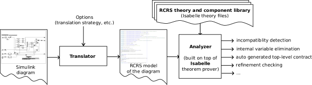
Figure 8: The RCRS toolset.

We implemented in Isabelle a shallow embedding [14] of the language introduced in §3. The advantage of a shallow embedding is that all datatypes of Isabelle are available for specification of components, and we can use the existing Isabelle mechanism for renaming bound variables in compositions. The disadvantage of this shallow embedding is that we cannot express Algorithm 7 within Isabelle (hence the “manual” proof that we provide for Theorem 11). A deep embedding, in which the syntax of components is defined as a datatype of Isabelle, is possible, and is left as an open future work direction.

We implemented Algorithm 7 in SML, the meta-language of Isabelle. The SML program takes as input a component $C$ and returns not only a simplified atomic component $\mathbf{atomic}(C)$, but also a proved Isabelle theorem of the fact $C\equiv\mathbf{atomic}(C)$. The simplification program, as well as a number of other procedures to perform compatibility checking, validity checking, etc., form what we call the Analyzer in Fig. 8.

The Translator takes as input a Simulink model and produces an RCRS/Isabelle theory file containing: (1) the definition of all atomic and composite components representing the Simulink diagram; and (2) embedded bottom-up simplification procedures and the corresponding correctness theorems. By running this theory file in Isabelle, we obtain an atomic component corresponding to the top-level Simulink model, equivalent to the original composite component. As a special case, if the Simulink diagram contains inconsistencies (e.g., division by zero), these are detected by obtaining $\mathsf{Fail}$ as the top-level atomic component. The error can be localized by finding earlier points in the Simulink hierarchy (subsystems) which already resulted in $\mathsf{Fail}$.

As mentioned earlier, how to obtain a composite component from a graphical block diagram is an interesting problem. This problem is studied in depth in [31], where several translation strategies are proposed. These various strategies all yield semantically equivalent components, but with different trade-offs in terms of size, readability, effectiveness of the simplification procedures, and so on. The Translator implements all these translation strategies, allowing the user to explore these trade-offs. Further details on the translation problem are provided in [31, 65]. A proof that the translation strategies yield semantically equivalent components is provided in [64]. This proof, which has been formalized in Isabelle, is a non-trivial result: the entire formalization of the translation algorithms and the proof is 13579 lines of Isabelle code.

We have used the RCRS toolset on several case studies, including a real-life benchmark provided by the Toyota motor company. The benchmark involves a Fuel Control System (FCS) described in [45, 46]. FCS aims at controlling the air mass and injected fuel in a car engine such that their ratio is always optimal. This problem has important implications on lowering pollution and costs by improving the engine performance. Toyota has made several versions of FCS publicly available as Simulink models at https://cps-vo.org/group/ARCH/benchmarks.

We have used the RCRS toolset to process two of the three Simulink models in the FCS benchmark suite (the third model contains blocks that are currently not implemented in the RCRS component library). A typical model in this set has a 3-layer hierarchy with a total of 104 Simulink block instances (97 basic blocks and 7 subsystems), and 101 connections out of which 8 are feedbacks. Each basic Simulink block is modeled in our framework by an atomic STS component (possibly stateless). These atomic STS components are created once, and form part of the RCRS implementation, which is reused for different Simulink models. The particular FCS diagram is translated into RCRS using the Translator, and simplified within Isabelle using our SML simplification procedure. After simplification, we obtain an atomic deterministic STS component with no inputs, 7 outputs, and 14 state variables. Its contract (which is 8337 characters long) includes a condition on the state variables, in particular, that a certain state variable must always be non-negative (as its value is fed into a square-root block). This condition makes it not immediately obvious that the whole system is valid (i.e., not $\mathsf{Fail}$). However, we can show after applying the transformation $\mathtt{sts}2\mathtt{qltl}$ that the resulting formula is satisfiable, which implies that the original model is consistent (i.e., no connections result in incompatibilities, there are no divisions by zero, etc.). This illustrates the use of RCRS as a powerful static analysis tool. More details on the FCS case study are provided in [31, 65, 32].

7 Related Work

Several formal compositional frameworks exist in the literature. Most closely related to RCRS are the frameworks of FOCUS [15], input-output automata [54], reactive modules [6], interface automata [22], and Dill’s trace theory [29]. RCRS shares with these frameworks many key compositionality principles, such as the notion of refinement. At the same time, RCRS differs and complements these frameworks in important ways. Specifically, FOCUS, IO-automata, and reactive modules, are limited to input-receptive systems, while RCRS is explicitly designed to handle non-input-receptive specifications. The benefits of non-input-receptiveness are discussed extensively in [79] and will not be repeated here. Interface automata are a low-level formalism whereas RCRS specifications and reasoning are symbolic. For instance, in RCRS one can naturally express systems with infinite state-spaces, input-spaces, or output-spaces. (Such systems can even be handled automatically, provided the corresponding logic they are expressed in is decidable.) Both interface automata and Dill’s trace theory use a single form of asynchronous parallel composition, whereas RCRS has three primitive composition operators (serial, parallel, feedback) with synchronous semantics.

Our work adapts and extends to the reactive system setting many of the ideas developed previously in a long line of research on correctness and compositionality for sequential programs. This line of research goes back to the works of Floyd, Hoare, Dijkstra, and Wirth, on formal program semantics, weakest preconditions, program development by stepwise refinement, and so on [34, 43, 27, 81]. It also goes back to game-theoretic semantics of sequential programs as developed in the original refinement calculus [10], as well as to contract-based design [57]. Many of the concepts used in our work are in spirit similar to those used in the above works. For instance, an input-output formula $\phi$ used in an atomic component in our language can be seen as a contract between the environment of the component and the component itself: the environment must satisfy the contract by providing to the component legal inputs, and the component must in turn provide legal outputs (for those inputs). On the other hand, several of the concepts used here come from the world of reactive systems and as such do not have a direct correspondence in the world of sequential programs. For instance, this is the case with feedback composition.

RCRS extends refinement calculus from predicate to property transformers. Extensions of refinement calculus to infinite behaviors have also been proposed in the frameworks of action systems [11], fair action systems [12], and Event B [3]. These frameworks use predicate (not property) transformers as semantic foundation; they can handle certain property patterns (e.g., fairness) by providing proof rules for these properties, but they do not treat livenes and LTL properties in general [12, 82, 42]. The Temporal Logic of Actions [49] can be used to specify liveness properties, but does not distinguish between inputs and outputs, and as such cannot express non-input-receptive components.

Our specifications can be seen as “rich”, behavioral types [50, 22]. Indeed, our work is closely related to programming languages and type theory, specifically, refinement types [35], behavioral types [60, 51, 26], and liquid types [69].

Behavioral type frameworks have also been proposed in reactive system settings. In the SimCheck framework [70], Simulink blocks are annotated with constraints on input and output variables, much like stateless components in RCRS. RCRS is more general as it also allows to specify stateful components. RCRS is also a more complete compositional framework, with composition operators and refinement, which are not considered in [70]. Other behavioral type theories for reactive systems have been proposed in [23, 18, 30]. Compared to RCRS, these works are less general. In particular, [23, 30] are limited to specifications which separate the assumptions on the inputs from the guarantees on the outputs, and as such cannot capture input-output relations. [18] considers a synchronous model which allows to specify legal values of inputs and outputs at the next step, given the current state. This model does not allow to capture relations between inputs and outputs within the same step, which RCRS allows.

Our work is related to formal verification frameworks for hybrid systems [5]. Broadly speaking, these can be classified into frameworks following a model-checking approach, which typically use automata-based specification languages and state-space exploration techniques, and those following a theorem-proving approach, which typically use logic-based specifications. More closely related to RCRS are the latter, among which, CircusTime [17], KeYmaera [37], and the PVS-based approach in [2]. CircusTime can handle a larger class of Simulink diagrams than the current implementation of RCRS. In particular, CircusTime can handle multi-rate diagrams, where different parts of the model work at different rates (periods). On the other hand, CircusTime is based on predicate (not property) transformers, and as such cannot handle liveness properties. KeYmaera is a theorem prover based on differential dynamic logic [62], which is itself based on dynamic logic [39]. The focus of both KeYmaera and the work in [2] is verification, and not compositionality. For instance, these works do not distinguish between inputs and outputs and do not investigate considerations such as input-receptiveness. The work of [68] distinguishes inputs and outputs, but provides a system model where the output relation is separated from the transition relation, and where the output relation is assumed to be total, meaning that there exists an output for every input and current state combination. This does not allow to specify non-input-receptive stateless components, such as for example the $\mathtt{Div}$ component from §3.

Our component algebra is similar to the algebra of flownomials [77] and to the relational model for non-deterministic dataflow [41]. In [20], graphs and graph operations which can be viewed as block diagrams are represented by algebraic expressions and operations, and a complete equational axiomatization of the equivalence of the graph expressions is given. This is then applied to flow-charts as investigated in [72]. The translation of block diagrams in general and Simulink in particular has been treated in a large number of papers, with various goals, including verification and code generation (e.g., see [80, 56, 19, 52, 73, 13, 83, 84, 85, 58]). Although we share several of the ideas of the above works, our main goal here is not to formalize the language of block diagrams, neither their translation to other formalisms, but to provide a complete compositional framework for reasoning about reactive systems.

RCRS is naturally related to compositional verification frameworks, such as [38, 1, 55, 74, 40, 24, 25]. In particular, compositional verification frameworks often make use of a refinement relation such as trace inclusion or simulation [74, 40]. However, the focus of these frameworks is different than that of RCRS. In compositional verification, the focus is to “break down” a large (and usually computationally expensive) verification task into smaller (and hopefully easier to calculate) subtasks. For this purpose, compositional verification frameworks employ several kinds of decomposition rules. An example of such a rule is the so-called precongruence rule (i.e., preservation of refinement by composition): if $P_{1}$ refines $Q_{1}$, and $P_{2}$ refines $Q_{2}$, then the composition $P_{1}\|P_{2}$ refines $Q_{1}\|Q_{2}$. This, together with preservation of properties by refinement, allows us to conclude that $P_{1}\|P_{2}$ satisfies some property $\phi$, provided we can prove that $Q_{1}\|Q_{2}$ satisfies $\phi$. The latter might be a simpler verification task, if $Q_{1}$ and $Q_{2}$ are smaller than $P_{1}$ and $P_{2}$. The essence of compositional verification is in finding such abstract versions $Q_{1}$ and $Q_{2}$ of the concrete processes in question, $P_{1}$ and $P_{2}$, and employing decomposition rules like the one above in the hope of making verification simpler. RCRS can also be used for compositional verification: indeed, RCRS provides both the precongruence rule, and preservation of properties by refinement. Note that, in traditional settings, precongruence is not always powerful enough, and for this reason most compositional verification frameworks employ more complex decomposition rules (e.g., see [59]). In settings which allow non-input-receptive components, such as ours, there are indications that the precongruence rule is sufficient for compositional verification purposes [75], although more work is required to establish this in the specific context of RCRS. Such work is beyond the scope of the current paper. We also note that, beyond compositional verification with precongruence, RCRS provides a behavioral type theory which allows to state system properties such as compatibility, which is typically not available in compositional verification frameworks.

Refinement can be seen as the inverse of abstraction, and as such our framework is related to general frameworks such as abstract interpretation [21]. Several abstractions have been proposed in reactive system settings, including relational abstractions for hybrid systems, which are related to Simulink [71]. The focus of these works is verification, and abstraction is used as a mechanism to remove details from the model that make verification harder. In RCRS, the simplification procedure that we employ can be seen as an abstraction process, as it eliminates internal variable information. However, RCRS simplification is an exact abstraction, in the sense that it does not lose any information: the final system is equivalent to the original one, and not an over- or under-approximation, as is usually the case with typical abstractions for verification purposes.

8 Conclusion

We presented RCRS, a compositional framework for modeling and reasoning about reactive systems. This paper focuses on the theory and methodology of RCRS, its formal semantics, and techniques for symbolic and computer-aided reasoning.

RCRS is an ongoing project, and a number of problems remain open. Future work directions include:

• An extension of the framework to systems with algebraic loops, which necessitates handling instantaneous feedback. Here, the preliminary ideas of [67] can be helpful in defining the semantics of instantaneous feedback. However, [67] does not provide solutions on how to obtain symbolic closed-form expression for the feedback of general components.

• Extension of the results of §5.5 to general components, possibly non-deterministic or non-decomposable.

• An extension of the framework to acausal systems, i.e., systems without a clear distinction of inputs and outputs [36].

• The development of better symbolic reasoning techniques, such as simplification of logical formulas, decision procedures, etc.

References

- [1] M. Abadi and L. Lamport. Conjoining specifications. ACM Trans. Program. Lang. Syst., 17(3):507–535, 1995.
- [2] E. Ábrahám-Mumm, M. Steffen, and U. Hannemann. Verification of hybrid systems: Formalization and proof rules in PVS. In 7th Intl. Conf. Engineering of Complex Computer Systems (ICECCS 2001), pages 48–57, 2001.
- [3] J.-R. Abrial. Modeling in Event-B: System and Software Engineering. Cambridge University Press, New York, NY, USA, 1st edition, 2010.
- [4] B. Alpern and F. B. Schneider. Defining liveness. Information Processing Letters, 21(4):181 – 185, 1985.
- [5] R. Alur, C. Courcoubetis, N. Halbwachs, T. Henzinger, P. Ho, X. Nicollin, A. Olivero, J. Sifakis, and S. Yovine. The algorithmic analysis of hybrid systems. Theoretical Computer Science, 138:3–34, 1995.
- [6] R. Alur and T. Henzinger. Reactive modules. Formal Methods in System Design, 15:7–48, 1999.
- [7] R. Alur, T. Henzinger, O. Kupferman, and M. Vardi. Alternating refinement relations. In CONCUR’98, volume 1466 of LNCS. Springer, 1998.
- [8] R. J. Back. Correctness preserving program refinements: proof theory and applications, volume 131 of Mathematical Centre Tracts. Mathematisch Centrum, Amsterdam, 1980.
- [9] R.-J. Back and M. Butler. Exploring summation and product operators in the refinement calculus, pages 128–158. Springer Berlin Heidelberg, Berlin, Heidelberg, 1995.
- [10] R.-J. Back and J. von Wright. Refinement Calculus: A Systematic Introduction. Springer, 1998.
- [11] R.-J. Back and J. Wright. Trace refinement of action systems. In B. Jonsson and J. Parrow, editors, CONCUR ’94: Concurrency Theory, volume 836 of Lecture Notes in Computer Science, pages 367–384. Springer Berlin Heidelberg, 1994.
- [12] R.-J. Back and Q. Xu. Refinement of fair action systems. Acta Informatica, 35(2):131–165, 1998.
- [13] P. Boström. Contract-Based Verification of Simulink Models. In S. Qin and Z. Qiu, editors, Formal Methods and Software Engineering, volume 6991 of Lecture Notes in Computer Science, pages 291–306. Springer Berlin Heidelberg, 2011.
- [14] R. J. Boulton, A. Gordon, M. J. C. Gordon, J. Harrison, J. Herbert, and J. V. Tassel. Experience with embedding hardware description languages in HOL. In IFIP TC10/WG 10.2 Intl. Conf. on Theorem Provers in Circuit Design, pages 129–156. North-Holland Publishing Co., 1992.
- [15] M. Broy and K. Stølen. Specification and development of interactive systems: focus on streams, interfaces, and refinement. Springer, 2001.
- [16] R. Cavada, A. Cimatti, M. Dorigatti, A. Griggio, A. Mariotti, A. Micheli, S. Mover, M. Roveri, and S. Tonetta. The nuxmv symbolic model checker. In A. Biere and R. Bloem, editors, Computer Aided Verification: 26th International Conference, CAV 2014,, pages 334–342, Cham, 2014. Springer.
- [17] A. L. C. Cavalcanti, A. Mota, and J. C. P. Woodcock. Simulink timed models for program verification. In Z. Liu, J. C. P. Woodcock, and H. Zhu, editors, Theories of Programming and Formal Methods - Essays Dedicated to Jifeng He on the Occasion of His 70th Birthday, volume 8051 of Lecture Notes in Computer Science, pages 82–99. Springer, 2013.
- [18] A. Chakrabarti, L. de Alfaro, T. Henzinger, and F. Mang. Synchronous and bidirectional component interfaces. In CAV, LNCS 2404, pages 414–427. Springer, 2002.
- [19] C. Chen, J. S. Dong, and J. Sun. A formal framework for modeling and validating Simulink diagrams. Formal Aspects of Computing, 21(5):451–483, 2009.
- [20] B. Courcelle. A representation of graphs by algebraic expressions and its use for graph rewriting systems. In H. Ehrig, M. Nagl, G. Rozenberg, and A. Rosenfeld, editors, Graph-Grammars and Their Application to Computer Science, 3rd International Workshop, Warrenton, Virginia, USA, December 2-6, 1986, volume 291 of Lecture Notes in Computer Science, pages 112–132. Springer, 1986.
- [21] P. Cousot and R. Cousot. Abstract interpretation: a unified lattice model for static analysis of programs by construction or approximation of fixpoints. In 4th ACM Symp. POPL, 1977.
- [22] L. de Alfaro and T. Henzinger. Interface automata. In Foundations of Software Engineering (FSE). ACM Press, 2001.
- [23] L. de Alfaro and T. Henzinger. Interface theories for component-based design. In EMSOFT’01. Springer, LNCS 2211, 2001.
- [24] W. de Roever, H. Langmaack, and A. E. Pnueli. Compositionality: The Significant Difference. LNCS. Springer, 1998.
- [25] W.-P. de Roever, F. de Boer, U. Hanneman, J. Hooman, Y. Lakhnech, M. Poel, and J. Zwiers. Concurrency Verification: Introduction to Compositional and Non-compositional Methods. Cambridge University Press, 2012.
- [26] K. Dhara and G. Leavens. Forcing behavioral subtyping through specification inheritance. In ICSE’96: 18th Intl. Conf. on Software Engineering, pages 258–267. IEEE Computer Society, 1996.
- [27] E. Dijkstra. Notes on structured programming. In O. Dahl, E. Dijkstra, and C. Hoare, editors, Structured programming, pages 1–82. Academic Press, London, UK, 1972.
- [28] E. Dijkstra. Guarded commands, nondeterminacy and formal derivation of programs. Comm. ACM, 18(8):453–457, 1975.
- [29] D. Dill. Trace theory for automatic hierarchical verification of speed-independent circuits. MIT Press, Cambridge, MA, USA, 1987.
- [30] L. Doyen, T. Henzinger, B. Jobstmann, and T. Petrov. Interface theories with component reuse. In 8th ACM & IEEE International conference on Embedded software, EMSOFT, pages 79–88, 2008.
- [31] I. Dragomir, V. Preoteasa, and S. Tripakis. Compositional Semantics and Analysis of Hierarchical Block Diagrams. In SPIN, pages 38–56. Springer, 2016.
- [32] I. Dragomir, V. Preoteasa, and S. Tripakis. The Refinement Calculus of Reactive Systems Toolset. CoRR, abs/1710.08195, 2017.
- [33] I. Dragomir, V. Preoteasa, and S. Tripakis. The Refinement Calculus of Reactive Systems Toolset. In TACAS, 2018.
- [34] R. Floyd. Assigning meanings to programs. In In. Proc. Symp. on Appl. Math. 19, pages 19–32. American Mathematical Society, 1967.
- [35] T. Freeman and F. Pfenning. Refinement Types for ML. SIGPLAN Not., 26(6):268–277, May 1991.
- [36] P. Fritzson. Principles of Object-Oriented Modeling and Simulation with Modelica 3.3: A Cyber-Physical Approach. Wiley, 2 edition, 2014.
- [37] N. Fulton, S. Mitsch, J.-D. Quesel, M. Völp, and A. Platzer. KeYmaera X: An axiomatic tactical theorem prover for hybrid systems. In A. P. Felty and A. Middeldorp, editors, CADE, volume 9195 of LNCS, pages 527–538. Springer, 2015.
- [38] O. Grumberg and D. Long. Model checking and modular verification. ACM Trans. Program. Lang. Syst., 16(3):843–871, 1994.
- [39] D. Harel, J. Tiuryn, and D. Kozen. Dynamic Logic. MIT Press, 2000.
- [40] T. Henzinger, S. Qadeer, and S. Rajamani. You assume, we guarantee: Methodology and case studies. In CAV’98, volume 1427 of LNCS. Springer-Verlag, 1998.
- [41] T. T. Hildebrandt, P. Panangaden, and G. Winskel. A relational model of non-deterministic dataflow. Mathematical Structures in Computer Science, 14(5):613–649, 10 2004.
- [42] T. S. Hoang and J.-R. Abrial. Reasoning About Liveness Properties in Event-B. In Proceedings of the 13th International Conference on Formal Methods and Software Engineering, ICFEM’11, pages 456–471, Berlin, Heidelberg, 2011. Springer-Verlag.
- [43] C. A. R. Hoare. An axiomatic basis for computer programming. Comm. ACM, 12(10):576–580, 1969.
- [44] C. A. R. Hoare. Proof of correctness of data representations. Acta Informatica, 1(4), Dec. 1972.
- [45] X. Jin, J. Deshmukh, J. Kapinski, K. Ueda, and K. Butts. Benchmarks for model transformations and conformance checking. In 1st Intl. Workshop on Applied Verification for Continuous and Hybrid Systems (ARCH), 2014.
- [46] X. Jin, J. V. Deshmukh, J. Kapinski, K. Ueda, and K. Butts. Powertrain Control Verification Benchmark. In Proceedings of the 17th International Conference on Hybrid Systems: Computation and Control, HSCC’14, pages 253–262. ACM, 2014.
- [47] Y. Kesten, Z. Manna, and A. Pnueli. Temporal verification of simulation and refinement. In J. W. de Bakker, W. P. de Roever, and G. Rozenberg, editors, A Decade of Concurrency Reflections and Perspectives: REX School/Symposium, pages 273–346. Springer, 1994.
- [48] Y. Kesten and A. Pnueli. Complete Proof System for QPTL. Journal of Logic and Computation, 12(5):701, 2002.
- [49] L. Lamport. The temporal logic of actions. ACM Trans. Program. Lang. Syst., 16(3):872–923, May 1994.
- [50] E. Lee and Y. Xiong. System-level types for component-based design. In EMSOFT’01: 1st Intl. Workshop on Embedded Software, pages 237–253. Springer, 2001.
- [51] B. Liskov and J. Wing. A behavioral notion of subtyping. ACM Trans. Program. Lang. Syst., 16(6):1811–1841, 1994.
- [52] R. Lublinerman, C. Szegedy, and S. Tripakis. Modular code generation from synchronous block diagrams – modularity vs. code size. In 36th ACM SIGPLAN-SIGACT Symposium on Principles of Programming Languages (POPL’09), pages 78–89. ACM, Jan. 2009.
- [53] R. Lublinerman and S. Tripakis. Modularity vs. reusability: Code generation from synchronous block diagrams. In Design, Automation, and Test in Europe (DATE’08), pages 1504–1509. ACM, Mar. 2008.
- [54] N. Lynch and M. Tuttle. An introduction to input/output automata. CWI Quarterly, 2:219–246, 1989.
- [55] K. McMillan. A compositional rule for hardware design refinement. In Computer Aided Verification (CAV’97), volume 1254 of LNCS. Springer-Verlag, 1997.
- [56] B. Meenakshi, A. Bhatnagar, and S. Roy. Tool for Translating Simulink Models into Input Language of a Model Checker. In Formal Methods and Software Engineering, volume 4260 of LNCS, pages 606–620. Springer, 2006.
- [57] B. Meyer. Applying “Design by Contract”. Computer, 25(10):40–51, 1992.
- [58] S. Minopoli and G. Frehse. SL2SX Translator: From Simulink to SpaceEx Verification Tool. In 19th ACM International Conference on Hybrid Systems: Computation and Control (HSCC), 2016.
- [59] K. S. Namjoshi and R. J. Trefler. On the completeness of compositional reasoning methods. ACM Trans. Comput. Logic, 11(3), 2010.
- [60] O. Nierstrasz. Regular types for active objects. SIGPLAN Not., 28(10):1–15, 1993.
- [61] T. Nipkow, L. C. Paulson, and M. Wenzel. Isabelle/HOL — A Proof Assistant for Higher-Order Logic. LNCS 2283. Springer, 2002.
- [62] A. Platzer. Differential dynamic logic for hybrid systems. J. Autom. Reas., 41(2):143–189, 2008.
- [63] A. Pnueli. The Temporal Logic of Programs. In 18th Annual Symposium on Foundations of Computer Science, Providence, Rhode Island, USA, 31 October - 1 November 1977, pages 46–57. IEEE Computer Society, 1977.
- [64] V. Preoteasa, I. Dragomir, and S. Tripakis. A nondeterministic and abstract algorithm for translating hierarchical block diagrams. CoRR, abs/1611.01337, 2016.
- [65] V. Preoteasa, I. Dragomir, and S. Tripakis. Type Inference of Simulink Hierarchical Block Diagrams in Isabelle. In 37th IFIP WG 6.1 International Conference on Formal Techniques for Distributed Objects, Components, and Systems (FORTE), 2017.
- [66] V. Preoteasa and S. Tripakis. Refinement calculus of reactive systems. In Embedded Software (EMSOFT), 2014 International Conference on, pages 1–10, Oct 2014.
- [67] V. Preoteasa and S. Tripakis. Towards Compositional Feedback in Non-Deterministic and Non-Input-Receptive Systems. In 31st Annual ACM/IEEE Symposium on Logic in Computer Science (LICS), 2016.
- [68] G. Reissig, A. Weber, and M. Rungger. Feedback refinement relations for the synthesis of symbolic controllers. IEEE Trans. Automat. Contr., 62(4):1781–1796, 2017.
- [69] P. M. Rondon, M. Kawaguci, and R. Jhala. Liquid types. In 29th ACM SIGPLAN Conference on Programming Language Design and Implementation, PLDI ’08, pages 159–169, New York, NY, USA, 2008. ACM.
- [70] P. Roy and N. Shankar. SimCheck: An expressive type system for Simulink. In C. Muñoz, editor, 2nd NASA Formal Methods Symposium (NFM 2010), NASA/CP-2010-216215, pages 149–160, Langley Research Center, Hampton VA 23681-2199, USA, Apr. 2010. NASA.
- [71] S. Sankaranarayanan and A. Tiwari. Relational abstractions for continuous and hybrid systems. In Computer Aided Verification: 23rd International Conference, CAV 2011, pages 686–702. Springer, 2011.
- [72] H. Schmeck. Algebraic characterization of reducible flowcharts. Journal of Computer and System Sciences, 27(2):165 – 199, 1983.
- [73] V. Sfyrla, G. Tsiligiannis, I. Safaka, M. Bozga, and J. Sifakis. Compositional translation of Simulink models into synchronous BIP. In Industrial Embedded Systems (SIES), 2010 International Symposium on, pages 217–220, July 2010.
- [74] N. Shankar. Lazy compositional verification. In COMPOS’97: Revised Lectures from the International Symposium on Compositionality: The Significant Difference, pages 541–564, London, UK, 1998. Springer-Verlag.
- [75] A. Siirtola, S. Tripakis, and K. Heljanko. When do we not need complex assume-guarantee rules? ACM Trans. Embed. Comput. Syst., 16(2):48:1–48:25, Jan. 2017.
- [76] A. P. Sistla, M. Y. Vardi, and P. Wolper. The Complementation Problem for Büchi Automata with Applications to Temporal Logic. Theoretical Computer Science, 49:217–237, 1987.
- [77] G. Stefănescu. Network Algebra. Springer-Verlag New York, Inc., Secaucus, NJ, USA, 2000.
- [78] S. Tripakis, B. Lickly, T. Henzinger, and E. Lee. On Relational Interfaces. In Proceedings of the 9th ACM & IEEE International Conference on Embedded Software (EMSOFT’09), pages 67–76. ACM, 2009.
- [79] S. Tripakis, B. Lickly, T. A. Henzinger, and E. A. Lee. A Theory of Synchronous Relational Interfaces. ACM Trans. Program. Lang. Syst., 33(4):14:1–14:41, July 2011.
- [80] S. Tripakis, C. Sofronis, P. Caspi, and A. Curic. Translating Discrete-time Simulink to Lustre. ACM Trans. Embed. Comput. Syst., 4(4):779–818, Nov. 2005.
- [81] N. Wirth. Program development by stepwise refinement. Comm. ACM, 14(4):221–227, 1971.
- [82] D. Yadav and M. Butler. Verification of liveness properties in distributed systems. In Contemporary Computing, volume 40 of Communications in Computer and Information Science, pages 625–636. Springer Berlin Heidelberg, 2009.
- [83] C. Yang and V. Vyatkin. Transformation of Simulink models to IEC 61499 Function Blocks for verification of distributed control systems. Control Engineering Practice, 20(12):1259–1269, 2012.
- [84] C. Zhou and R. Kumar. Semantic Translation of Simulink Diagrams to Input/Output Extended Finite Automata. Discrete Event Dynamic Systems, 22(2):223–247, 2012.
- [85] L. Zou, N. Zhany, S. Wang, M. Franzle, and S. Qin. Verifying Simulink diagrams via a Hybrid Hoare Logic Prover. In Embedded Software (EMSOFT), Sept 2013.