The Galactic Dependencies Treebanks:
Getting More Data by Synthesizing New Languages

Abstract

We release Galactic Dependencies 1.0—a large set of synthetic languages not found on Earth, but annotated in Universal Dependencies format. This new resource aims to provide training and development data for NLP methods that aim to adapt to unfamiliar languages. Each synthetic treebank is produced from a real treebank by stochastically permuting the dependents of nouns and/or verbs to match the word order of other real languages. We discuss the usefulness, realism, parsability, perplexity, and diversity of the synthetic languages. As a simple demonstration of the use of Galactic Dependencies, we consider single-source transfer, which attempts to parse a real target language using a parser trained on a “nearby” source language. We find that including synthetic source languages somewhat increases the diversity of the source pool, which significantly improves results for most target languages.

1 Motivation

Some potential NLP tasks have very sparse data by machine learning standards, as each of the IID training examples is an entire language. For instance:

• typological classification of a language on various dimensions;

• adaptation of any existing NLP system to new, low-resource languages;

• induction of a syntactic grammar from text;

• discovery of a morphological lexicon from text;

• other types of unsupervised discovery of linguistic structure.

Given a corpus or other data about a language, we might aim to predict whether it is an SVO language, or to learn to pick out its noun phrases. For such problems, a single training or test example corresponds to an entire human language.

Unfortunately, we usually have only from 1 to 40 languages to work with. In contrast, machine learning methods thrive on data, and recent AI successes have mainly been on tasks where one can train richly parameterized predictors on a huge set of IID (input, output) examples. Even 7,000 training examples—one for each language or dialect on Earth—would be a small dataset by contemporary standards.

As a result, it is challenging to develop systems that will discover structure in new languages in the same way that an image segmentation method, for example, will discover structure in new images. The limited resources even make it challenging to develop methods that handle new languages by unsupervised, semi-supervised, or transfer learning. Some such projects evaluate their methods on new sentences of the same languages that were used to develop the methods in the first place—which leaves one worried that the methods may be inadvertently tuned to the development languages and may not be able to discover correct structure in other languages. Other projects take care to hold out languages for evaluation Spitkovsky (2013); Cotterell et al. (2015), but then are left with only a few development languages on which to experiment with different unsupervised methods and their hyperparameters.

If we had many languages, then we could develop better unsupervised language learners. Even better, we could treat linguistic structure discovery as a supervised learning problem. That is, we could train a system to extract features from the surface of a language that are predictive of its deeper structure. Principles & Parameters theory Chomsky (1981) conjectures that such features exist and that the juvenile human brain is adapted to extract them.

Our goal in this paper is to release a set of about 50,000 high-resource languages that could be used to train supervised learners, or to evaluate less-supervised learners during development. These “unearthly” languages are intended to be at least similar to possible human languages. As such, they provide useful additional training and development data that is slightly out of domain (reducing the variance of a system’s learned parameters at the cost of introducing some bias). The initial release as described in this paper (version 1.0) is available at https://github.com/gdtreebank/gdtreebank. We plan to augment this dataset in future work (§8).

In addition to releasing thousands of treebanks, we provide scripts that can be used to “translate” other annotated resources into these synthetic languages. E.g., given a corpus of English sentences labeled with sentiment, a researcher could reorder the words in each English sentence according to one of our English-based synthetic languages, thereby obtaining labeled sentences in the synthetic language.

2 Related Work

Synthetic data generation is a well-known trick for effectively training a large model on a small dataset. Abu-Mostafa (1995) reviews early work that provided “hints” to a learning system in the form of virtual training examples. While datasets have grown in recent years, so have models: e.g., neural networks have many parameters to train. Thus, it is still common to create synthetic training examples—often by adding noise to real inputs or otherwise transforming them in ways that are expected to preserve their labels. Domains where it is easy to exploit these invariances include image recognition Simard et al. (2003); Krizhevsky et al. (2012), speech recognition Jaitly and Hinton (2013); Cui et al. (2015), information retrieval Vilares et al. (2011), and grammatical error correction Rozovskaya and Roth (2010).

Synthetic datasets have also arisen recently for semantic tasks in natural language processing. bAbI is a dataset of facts, questions, and answers, generated by random simulation, for training machines to do simple logic Weston et al. (2016). Hermann et al. (2015) generate reading comprehension questions and their answers, based on a large set of news-summarization pairs, for training machine readers. Serban et al. (2016) used RNNs to generate 30 million factoid questions about Freebase, with answers, for training question-answering systems. Wang et al. (2015) obtain data to train semantic parsers in a new domain by first generating synthetic (utterance, logical form) pairs and then asking human annotators to paraphrase the synthetic utterances into more natural human language.

In speech recognition, morphology-based “vocabulary expansion” creates synthetic word forms Rasooli et al. (2014); Varjokallio and Klakow (2016).

Machine translation researchers have often tried to automatically preprocess parse trees of a source language to more closely resemble those of the target language, using either hand-crafted or automatically extracted rules (Dorr et al., 2002; Collins et al., 2005, etc.; see review by Howlett and Dras, 2011).

3 Synthetic Language Generation

A treebank is a corpus of parsed sentences of some language. We propose to derive each synthetic treebank from some real treebank. By manipulating the existing parse trees, we obtain a useful corpus for our synthetic language—a corpus that is already tagged, parsed, and partitioned into training/development/test sets. Additional data in the synthetic language can be obtained, if desired, by automatically parsing additional real-language sentences and manipulating these trees in the same way.

[theme = simple] [column sep=.2em] $*$& DET & NOUN & PROPN & VERB & VERB & DET & ADJ & NOUN & ADV & PUNCT
ROOT & Every & move & Google & makes & brings & this & particular & future & closer & .
[arc angle=10]32det 63nsubj 54nsubj 35acl:rel 16root 97det 98amod 69dobj 610advmod 611punct Language Sentence English Every move Google makes brings this particular future closer. English[French/N] Every move Google makes brings this future particular closer. English[Hindi/V] Every move Google makes this particular future closer brings. English[French/N, Hindi/V] Every move Google makes this future particular closer brings.

Figure 1: The original UD tree for a short English sentence, and its “translations” into three synthetic languages, which are obtained by manipulating the tree. (Moved constituents are underlined.) Each language has a different distribution over surface part-of-speech sequences.

3.1 Method

We begin with the Universal Dependencies collection version 1.2 Nivre et al. (2015, 2016), or UD. This provides manually edge-labeled dependency treebanks in 37 real languages, in a consistent style and format—the Universal Dependencies format. An example appears in Figure 1.

In this paper, we select a substrate language $S$ represented in the UD treebanks, and systematically reorder the dependents of some nodes in the $S$ trees, to obtain trees of a synthetic language $S^{\prime}$.

Specifically, we choose a superstrate language $R_{\texttt{V}}$, and write $S^{\prime}=S[R_{\texttt{V}}/{\texttt{V}}]$ to denote a (projective) synthetic language obtained from $S$ by permuting the dependents of verbs (V) to match the ordering statistics of the $R_{\texttt{V}}$ treebanks. We can similarly permute the dependents of nouns (N). This permutes about 93% of $S$’s nodes (Table 2), as UD treats adpositions and conjunctions as childless dependents.

For example, English[French/N, Hindi/V] is a synthetic language based on an English substrate, but which adopts subject-object-verb (SOV) word order from the Hindi superstrate and noun-adjective word order from the French superstrate (Figure 1). Note that it still uses English lexical items.

Our terms “substrate” and “superstrate” are borrowed from the terminology of creoles, although our synthetic languages are unlike naturally occurring creoles. Our substitution notation $S^{\prime}=S[R_{\texttt{N}}/{\texttt{N}},R_{\texttt{V}}/{\texttt{V}}]$ is borrowed from the logic and programming languages communities.

3.2 Discussion

There may be more adventurous ways to manufacture synthetic languages (see §8 for some options). However, we emphasize that our current method is designed to produce fairly realistic languages.

First, we retain the immediate dominance structure and lexical items of the substrate trees, altering only their linear precedence relations. Thus each sentence remains topically coherent; nouns continue to be distinguished by case according to their role in the clause structure; wh-words continue to c-command gaps; different verbs (e.g., transitive vs. intransitive) continue to be associated with different subcategorization frames; and so on. These important properties would not be captured by a simple context-free model of dependency trees, which is why we modify real sentences rather than generating new sentences from such a model. In addition, our method obviously preserves the basic context-free properties, such as the fact that verbs typically subcategorize for one or two nominal arguments Naseem et al. (2010).

Second, by drawing on real superstrate languages, we ensure that our synthetic languages use plausible word orders. For example, if $R_{\texttt{V}}$ is a V2 language that favors SVO word order but also allows OVS, then $S^{\prime}$ will match these proportions. Similarly, $S^{\prime}$ will place adverbs in reasonable positions with respect to the verb.

We note, however, that our synthetic languages might violate some typological universals or typological tendencies. For example, $R_{\texttt{V}}$ might prescribe head-initial verb orderings while $R_{\texttt{N}}$ prescribes head-final noun orderings, yielding an unusual language. Worse, we could synthesize a language that uses free word order (from $R_{\texttt{V}}$) even though nouns (from $S$) are not marked for case. Such languages are rare, presumably for the functionalist reason that sentences would be too ambiguous. One could automatically filter out such an implausible language $S^{\prime}$, or downweight it, upon discovering that a parser for $S^{\prime}$ was much less accurate on held-out data than a comparable parser for $S$.

We also note that our reordering method (§4) does ignore some linguistic structure. For example, we do not currently condition the order of the dependent subtrees on their heaviness or on the length of resulting dependencies, and thus we will not faithfully model phenomena like heavy-shift Hawkins (1994); Eisner and Smith (2010). Nor will we model the relative order of adjectives. We also treat all verbs interchangeably, and thus use the same word orders—drawn from $R_{\texttt{V}}$—for both main clauses and embedded clauses. This means that we will never produce a language like German (which uses V2 order in main clauses and SOV order in embedded clauses), even if $R_{\texttt{V}}=\text{German}$. All of these problems could be addressed by enriching the features that are described in the next section.

4 Modeling Dependent Order

Let $X$ be a part-of-speech tag, such as Verb. To produce a dependency tree in language $S^{\prime}=S[R_{X}/X]$, we start with a projective dependency tree in language $S$. For each node $x$ in the tree that is tagged with $X$, we stochastically select a new ordering for its dependent nodes, including a position in this ordering for the head $x$ itself. Thus, if node $x$ has $n-1$ dependents, then we must sample from a probability distribution over $n!$ orderings.

Our job in this section is to define this probability distribution. Using $\pi=(\pi_{1},\ldots,\pi_{n})$ to denote an ordering of these $n$ nodes, we define a log-linear model over the possible values of $\pi$:

$$p_{\boldsymbol{\mathbf{\theta}}}(\pi\mid x)=\frac{1}{Z(x)}\exp\;\smashoperator[lr]{\sum_{1\leq i<j\leq n}^{}}\;{\boldsymbol{\mathbf{\theta}}}\cdot{\boldsymbol{\mathbf{f}}}(\pi,i,j)$$ (1)

Here $Z(x)$ is the normalizing constant for node $x$. ${\boldsymbol{\mathbf{\theta}}}$ is the parameter vector of the model. ${\boldsymbol{\mathbf{f}}}$ extracts a sparse feature vector that describes the ordered pair of nodes $\pi_{i},\pi_{j}$, where the ordering $\pi$ would place $\pi_{i}$ to the left of $\pi_{j}$.

4.1 Efficient sampling

To sample exactly from the distribution $p_{\boldsymbol{\mathbf{\theta}}}$, we must explicitly compute all $n!$ unnormalized probabilities and their sum $Z(x)$.

Fortunately, we can compute each unnormalized probability in just $O(1)$ amortized time, if we enumerate the $n!$ orderings $\pi$ using the Steinhaus-Johnson-Trotter algorithm Sedgewick (1977). This enumeration sequence has the property that any two consecutive permutations $\pi,\pi^{\prime}$ differ by only a single swap of some pair of adjacent nodes. Thus their probabilities are closely related: the sum in equation (1) can be updated in $O(1)$ time by subtracting ${\boldsymbol{\mathbf{\theta}}}\cdot{\boldsymbol{\mathbf{f}}}(\pi,i,i+1)$ and adding ${\boldsymbol{\mathbf{\theta}}}\cdot{\boldsymbol{\mathbf{f}}}(\pi^{\prime},i,i+1)$ for some $i$. The other $O(n^{2})$ summands are unchanged.

In addition, if $n\geq 8$, we avoid this computation by omitting the entire tree from our treebank; so we have at most $7!=5040$ summands.

4.2 Training parameters on a real language

Our feature functions (§4.4) are fixed over all languages. They refer to the 17 node labels (POS tags) and 40 edge labels (dependency relations) that are used consistently throughout the UD treebanks.

For each UD language $L$ and each POS tag $X$, we find parameters ${\boldsymbol{\mathbf{\theta}}}_{X}^{L}$ that globally maximize the unregularized log-likelihood:

$${\boldsymbol{\mathbf{\theta}}}_{X}^{L}=\operatorname*{argmax}_{\boldsymbol{\mathbf{\theta}}}\sum_{x}\log p_{\boldsymbol{\mathbf{\theta}}}(\pi_{x}\mid x)$$ (2)

Here $x$ ranges over all nodes tagged with $X$ in the projective training trees of the $L$ treebank, omitting nodes with $n\geq 7$ for speed.

The expensive part of this computation is the gradient of $\log Z(x)$, which is an expected feature vector. To compute this expectation efficiently, we again take care to loop over the permutations in Steinhaus-Johnson-Trotter order.

A given language $L$ may not use all of the tags and relations. Universal features that mention unused tags or relations do not affect (2), and their weights remain at 0 during training.

4.3 Setting parameters of a synthetic language

We use (1) to permute the $X$ nodes of substrate language $S$ into an order resembling superstrate language $R_{X}$. In essence, this applies the $R_{X}$ ordering model to out-of-domain data, since the $X$ nodes may have rather different sets of dependents in the $S$ treebank than in the $R_{X}$ treebank. We mitigate this issue in two ways.

First, our ordering model (1) is designed to be more robust to transfer than, say, a Markov model. The position of each node is influenced by all $n-1$ other nodes, not just by the two adjacent nodes. As a result, the burden of explaining the ordering is distributed over more features, and we hope some of these features will transfer to $S$. For example, suppose $R_{X}$ lacks adverbs and yet we wish to use ${\boldsymbol{\mathbf{\theta}}}_{X}^{R_{X}}$ to permute a sequence of $S$ that contains adverbs. Even though the resulting order must disrupt some familiar non-adverb bigrams by inserting adverbs, other features—which consider non-adjacent tags—will still favor an $R_{X}$-like order for the non-adverbs.

Second, we actually sample the reordering from a distribution $p_{\boldsymbol{\mathbf{\theta}}}$ with an interpolated parameter vector

$${\boldsymbol{\mathbf{\theta}}}={\boldsymbol{\mathbf{\theta}}}_{X}^{S^{\prime}}=(1-\lambda){\boldsymbol{\mathbf{\theta}}}_{X}^{R_{X}}+\lambda{\boldsymbol{\mathbf{\theta}}}_{X}^{S},$$

where $\lambda=0.05$. This gives a weighted product of experts, in which ties are weakly broken in favor of the substrate ordering. (Ties arise when $R_{X}$ is unfamiliar with some tags that appear in $S$, e.g., adverb.)

4.4 Feature Templates

We write $t_{i}$ for the POS tag of node $\pi_{i}$, and $r_{i}$ for the dependency relation of $\pi_{i}$ to the head node. If $\pi_{i}$ is itself the head, then necessarily $t_{i}=X$, and we specially define $r_{i}=\texttt{head}$.

In our feature vector ${\boldsymbol{\mathbf{f}}}(\pi,i,j)$, the features with the following names have value 1, while all others have value 0:

• L.$t_{i}$.$r_{i}$ and L.$t_{i}$ and L.$r_{i}$, provided that $r_{j}=\texttt{head}$. For example, L.ADJ will fire on each ADJ node to the left of the head.

• L.$t_{i}$.$r_{i}$.$t_{j}$.$r_{j}$ and L.$t_{i}$.$t_{j}$ and L.$r_{i}$.$r_{j}$, provided that $r_{i}\neq\texttt{head},r_{j}\neq\texttt{head}$. These features detect the relative order of two siblings.

• $d.t_{i}.r_{i}.t_{j}.r_{j}$, $d.t_{i}.t_{j}$, and $d.r_{i}.r_{j}$, where $d$ is l (left), m (middle), or r (right) according to whether the head position $h$ satisfies $i<j<h$, $i<h<j$, or $h<i<j$. For example, l.nsubj.dobj will fire on SOV clauses. This is a specialization of the previous feature, and is skipped if $i=h$ or $j=h$.

• A.$t_{i}$.$r_{i}$.$t_{j}$.$r_{j}$ and A.$t_{i}$.$t_{j}$ and A.$r_{i}$.$r_{j}$, provided that $j=i+1$. These “bigram features” detect two adjacent nodes. For this feature and the next one, we extend the summation in (1) to allow $0\leq i<j\leq n+1$, taking $t_{0}=r_{0}=\texttt{BOS}$ (“beginning of sequence”) and $t_{n+1}=r_{n+1}=\texttt{EOS}$ (“end of sequence”). Thus, a bigram feature such as A.DET.EOS would fire on DET when it falls at the end of the sequence.

• H.$t_{i}$.$r_{i}$.$t_{i+1}$.$r_{i+1}$.….$t_{j}$.$r_{j}$, provided that $i+2\leq j\leq i+4$. Among features of this form, we keep only the 10% that fire most frequently in the training data. These “higher-order $k$-gram” features memorize sequences of lengths 3 to 5 that are common in the language.

Notice that for each non-H feature that mentions both tags $t$ and relations $r$, we also defined two backoff features, omitting the $t$ fields or $r$ fields respectively.

Using the example from Figure 1, for subtree

[theme = simple] [column sep=.2em] DET & ADJ & NOUN
this & particular & future
31det 32amod

the features that fire are

Template	Features
L.$t_{i}$.$r_{i}$	L.DET.det, L.ADJ.amod
L.$t_{i}$.$r_{i}$.$t_{j}$.$r_{j}$	L.DET.det.ADJ.amod
$d$.$t_{i}$.$r_{i}$.$t_{j}$.$r_{j}$	l.DET.det.ADJ.amod
A.$t_{1}$.$r_{1}$.$t_{2}$.$r_{2}$	A.BOS.BOS.DET.det, A.DET.det.ADJ.amod, A.ADJ.amod.NOUN.head, A.NOUN.head.EOS.EOS

plus backoff features and H features (not shown).

5 The Resource

In Galactic Dependencies v1.0, or GD, we release real and synthetic treebanks based on UD v1.2. Each synthetic treebank is a modified work that is freely licensed under the same CC or GPL license as its substrate treebank. We provide all languages of the form $S$, $S[R_{\texttt{V}}/{\texttt{N}}]$, $S[R_{\texttt{N}}/{\texttt{V}}]$, and $S[R_{\texttt{N}}/{\texttt{N}},R_{\texttt{V}}/{\texttt{V}}]$, where the substrate $S$ and the superstrates $R_{\texttt{N}}$ and $R_{\texttt{V}}$ each range over the 37 available languages. ($R_{\texttt{N}}=S$ or $R_{\texttt{V}}=S$ gives “self-permutation”). This yields $37\times 38\times 38=53,428$ languages in total.

Each language is provided as a directory of 3 files: training, development, and test treebanks. The directories are systematically named: for example, English[French/N, Hindi/V] can be found in directory en$\sim$fr@N$\sim$hi@V.

Train	Dev	Test
cs, es, fr, hi, de, it, la_itt, no, ar, pt	en, nl, da, fi, got, grc, et, la_proiel, grc_proiel, bg	la, hr, ga, he, hu, fa, ta, cu, el, ro, sl, ja_ktc, sv, fi_ftb, id, eu, pl

Table 1: The 37 real UD languages. Following the usual setting of rich-to-poor transfer, we take the 10 largest non-English languages (left column) as our pool of real source languages, which we can combine to synthesize new languages. The remaining languages are our low-resource target languages. We randomly hold out 17 non-English languages (right column) as the test languages for our final result table. During development, we studied and graphed performance on the remaining 10 languages (middle column)—including English for interpretability.

Our treebanks provide alignment information, to facilitate error analysis as well as work on machine translation. Each word in a synthetic sentence is annotated with its original position in the substrate sentence. Thus, all synthetic treebanks derived from the same substrate treebank are node-to-node aligned to the substrate treebank and hence to one another.

In addition to the generated data, we also provide the parameters $\theta_{X}^{L}$ of our ordering models; code for training new ordering models; and code for producing new synthetic trees and synthetic languages. Our code should produce reproducible results across platforms, thanks to Java’s portability and our standard random number seed of 0.

lang	sents		tokens		$T$	UAS		$R$
ar	4K /	6K	119K /	226K	85%	72% /	69%	0.37
cs	5K /	7K	687K /	1173K	94%	81% /	78%	0.38
de	9K /	14K	136K /	270K	94%	84% /	80%	0.47
es	10K /	14K	211K /	382K	94%	85% /	82%	0.32
fr	8K /	15K	154K /	356K	95%	86% /	84%	0.27
hi	9K /	13K	160K /	281K	96%	82% /	82%	0.20
it	9K /	12K	144K /	249K	95%	87% /	84%	0.30
la_itt	7K /	15K	87K /	247K	90%	66% /	58%	0.72
no	11K /	16K	135K /	245K	93%	82% /	79%	0.31
pt	5K /	9K	87K /	202K	96%	86% /	84%	0.32

Table 2: Some statistics on the 10 real training languages. When two numbers are separated by “/”, the second represents the full UD treebank, and the first comes from our GD version, which discards non-projective trees and high-fanout trees ($n\geq 8$). UAS is the language’s parsability: the unlabeled attachment score on its dev sentences after training on its train sentences. $T$ is the percentage of GD tokens that are touched by reordering (namely N, V, and their dependents). $R\in[0,1]$ measures the freeness of the language’s word order, as the conditional cross-entropy of our trained ordering model $p_{\boldsymbol{\mathbf{\theta}}}$ relative to that of a uniform distribution: $R=\frac{H(\tilde{p},p_{\boldsymbol{\mathbf{\theta}}})}{H(\tilde{p},p_{\text{unif}})}=\frac{\operatorname*{mean}_{x}[-\log_{2}p_{\boldsymbol{\mathbf{\theta}}}(\pi^{*}(x)\mid x)]}{\operatorname*{mean}_{x}[-\log_{2}1/n(x)!]}$, where $x$ ranges over all N and V tokens in the dev sentences, $n(x)$ is 1 + the number of dependents of $x$, and $\pi^{*}(x)$ is the observed ordering at $x$.

6 Exploratory Data Analysis

How do the synthetic languages compare to the real ones? For analysis and experimentation, we partition the real UD languages into train/dev/test (Table 1). (This is orthogonal to the train/dev/test split of each language’s treebank.) Table 2 shows some properties of the real training languages.

In this section and the next, we use the Yara parser Rasooli and Tetreault (2015), a fast arc-eager transition-based projective dependency parser, with beam size of 8. We train only delexicalized parsers, whose input is the sequence of POS tags. Parsing accuracy is evaluated by the unlabeled attachment score (UAS), that is, the fraction of word tokens in held-out (dev) data that are assigned their correct parent. For language modeling, we train simple trigram backoff language models with add-1 smoothing, and we measure predictive accuracy as the perplexity of held-out (dev) data.

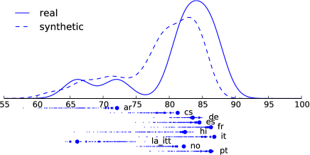
Figure 2: Parsability of real versus synthetic languages (defined as in Table 2). The upper graphs are kernel density estimates. Each lower graph is a 1-dimensional scatterplot, showing the parsability of some real language $S$ (large dot) and all its permuted versions, including the “self-permuted” languages $S[S/{\texttt{N}}]$ (diamond), $S[S/{\texttt{V}}]$ (square), and $S[S/{\texttt{N}},S/{\texttt{V}}]$ (medium dot).

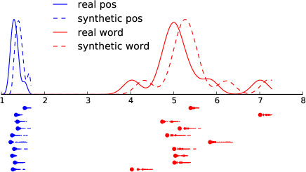
Figure 3: Perplexity of the POS tag sequence, as well as the word sequence, of real versus synthetic languages. Words with count $<10$ are mapped to an OOV symbol.

Figures 2–3 show how the parsability and perplexity of a real training language usually get worse when we permute it. We could have discarded low-parsability synthetic languages, on the functionalist grounds that they would be unlikely to survive as natural languages anywhere in the galaxy. However, the curves in these figures show that most synthetic languages have parsability and perplexity within the plausible range of natural languages, so we elected to simply keep all of them in our collection.

An interesting exception in Figure 2 is Latin (la_itt), whose poor parsability—at least by a delexicalized parser that does not look at word endings—may be due to its especially free word order (Table 2). When we impose another language’s more consistent word order on Latin, it becomes more parsable. Elsewhere, permutation generally hurts, perhaps because a real language’s word order is globally optimized to enhance parsability. It even hurts slightly when we randomly “self-permute” $S$ trees to use other word orders that are common in $S$ itself! Presumably this is because the authors of the original $S$ sentences chose, or were required, to order each constituent in a way that would enhance its parsability in context: see the last paragraph of §3.2.

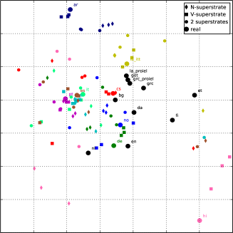
Figure 4: Each point represents a language. The color of a synthetic language is the same as its substrate language. Dev languages are shown in black. This 2-dimensional embedding was constructed using metric multidimensional scaling Borg and Groenen (2005) on a symmetrized version of our dissimilarity matrix (which is not itself a metric). The embedded distances are reasonably faithful to the symmetrized dissimilarities: metric MDS achieves a low value of 0.20 on its “stress” objective, and we find that Kendall’s tau = 0.76, meaning that if one pair of languages is displayed as farther apart than another, then in over $7/8$ of cases, that pair is in fact more dissimilar. Among the real languages, note the clustering of Italic languages (pt, es, fr, it), Germanic languages (de, no, en, nl, da), Slavic languages (cs, bg), and Uralic languages (et, fi). Outliers are Arabic (ar), the only Afroasiatic language here, and Hindi (hi), the only SOV language, whose permutations are less outré than it is.

Synthesizing languages is a balancing act. The synthetic languages are not useful if all of them are too conservatively close to their real sources to add diversity—or too radically different to belong in the galaxy of natural languages. Fortunately, we are at neither extreme. Figure 4 visualizes a small sample of 110 languages from our collection. For each ordered pair of languages $(S,T)$, we defined the dissimilarity $d(S,T)$ as the decrease in UAS when we parse the dev data of $T$ using a parser trained on $S$ instead of one trained on $T$. Small dissimilarity (i.e., good parsing transfer) translates to small distance in the figure. The figure shows that the permutations of a substrate language (which share its color) can be radically different from it, as we already saw above. Some may be unnatural, but others are similar to other real languages, including held-out dev languages. Thus Dutch (nl) and Estonian (et) have close synthetic neighbors within this small sample, although they have no close real neighbors.

7 An Experiment

We now illustrate the use of GD by studying how expanding the set of available treebanks can improve a simple NLP method, related to Figure 4.

7.1 Single-source transfer

Dependency parsing of low-resource languages has been intensively studied for years. A simple method is called “single-source transfer”: parsing a target language $T$ with a parser that was trained on a source language $S$, where the two languages are syntactically similar. Such single-source transfer parsers Ganchev et al. (2010); McDonald et al. (2011); Ma and Xia (2014); Guo et al. (2015); Duong et al. (2015); Rasooli and Collins (2015) are not state-of-the-art, but they have shown substantial improvements over fully unsupervised grammar induction systems Klein and Manning (2004); Smith and Eisner (2006); Spitkovsky et al. (2013).

It is permitted for $S$ and $T$ to have different vocabularies. The $S$ parser can nonetheless parse $T$ (as in Figure 4)—provided that it is a “delexicalized” parser that only cares about the POS tags of the input words. In this case, we require only that the target sentences have already been POS tagged using the same tagset as $S$: in our case, the UD tagset.

7.2 Experimental Setup

We evaluate single-source transfer when the pool of $m$ source languages consists of $n$ real UD languages, plus $m-n$ synthetic GD languages derived by “remixing” just these real languages. We try various values of $n$ and $m$, where $n$ can be as large as 10 (training languages from Table 1) and $m$ can be as large as $n\times(n+1)\times(n+1)\leq 1210$ (see §5).

Given a real target language $T$ from outside the pool, we select a single source language $S$ from the pool, and try to parse UD sentences of $T$ with a parser trained on $S$. We evaluate the results on $T$ by measuring the unlabeled attachment score (UAS), that is, the fraction of word tokens that were assigned their correct parent. In these experiments (unlike those of §6), we always evaluate fairly on $T$’s full dev or test set from UD—not just the sentences we kept for its GD version (cf. Table 2).

The hope is that a large pool will contain at least one language—real or synthetic—that is “close” to $T$. We have two ways of trying to select a source $S$ with this property:

Supervised selection selects the $S$ whose parser achieves the highest UAS on 100 training sentences of language $T$. This requires 100 good trees for $T$, which could be obtained with a modest investment—a single annotator attempting to follow the UD annotation standards in a consistent way on 100 sentences of $T$, without writing out formal $T$-specific guidelines. (There is no guarantee that selecting a parser on training data will choose well for the test sentences of $T$. We are using a small amount of data to select among many dubious parsers, many of which achieve similar results on the training sentences of $T$. Furthermore, in the UD treebanks, the test sentences of $T$ are sometimes drawn from a different distribution than the training sentences.)

Unsupervised selection selects the $S$ whose training sentences had the best “coverage” of the POS tag sequences in the actual data from $T$ that we aim to parse. More precisely, we choose the $S$ that maximizes $p_{S}($tag sequences from $T)$—in other words, the maximum-likelihood $S$—where $p_{S}$ is our trigram language model for the tag sequences of $S$. This approach is loosely inspired by Søgaard (2011).

7.3 Results

Our most complete visualization is Figure 5, which we like to call the “kite graph” for its appearance. We plot the UAS on the development treebank of $T$ as a function of $n$, $m$, and the selection method. As Appendix A details, each point on this graph is actually an average over 10,000 experiments that make random choices of $T$ (from the UD development languages), the $n$ real languages (from the UD training languages), and the $m-n$ synthetic languages (from the GD languages derived from the $n$ real languages). We see from the black lines that increasing the number of real languages $n$ is most beneficial. But crucially, when $n$ is fixed in practice, gradually increasing $m$ by remixing the real languages does lead to meaningful improvements. This is true for both selection methods. Supervised selection is markedly better than unsupervised.

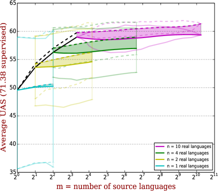
Figure 5: Comprehensive results for single-source transfer from a pool of $m$ languages (the horizontal axis) synthesized from $n$ real languages. For each color $1,2,\ldots,n$, the upper dashed line shows the UAS achieved by supervised selection; the lower solid line shows unsupervised selection; and the shaded area highlights the difference. The black dashed and solid lines connect the points where $m=n$, showing how rapidly UAS increases with $n$ when only real languages are used.
   Each point is the mean dev UAS over 10,000 experiments. We use paler lines in the same color and style to show the considerable variance of these UAS scores. These essentially delimit the interdecile range from the 10th to the 90th percentile of UAS score. However, if the plot shows a mean of 57, an interdecile range from 53 to 61 actually means that the middle 80% of experiments were within $\pm 4$ percentage points of the mean UAS for their target language. (In other words, before computing this range, we adjust each UAS score for target $T$ by subtracting the mean UAS from the experiments with target $T$, and adding back the mean UAS from all 10,000 experiments (e.g., 57).)
   Notice that on the $n=10$ curve, there is no variation among experiments either at the minimum $m$ (where the pool always consists of all 10 real languages) or at the maximum $m$ (where the pool always consists of all 1210 galactic languages).

The “selection graph” in Figure 6 visualizes the same experiments in a different way. Here we ask about the fraction of experiments in which using the full pool of $m$ source languages was strictly better than using only the $n$ real languages. We find that when $m$ has increased to its maximum, the full pool nearly always contains a synthetic source language that gets better results than anything in the real pool. After all, our generation of “random” languages is a scattershot attempt to hit the target: the more languages we generate, the higher our chances of coming close. However, our selection methods only manage to pick a better language in about 60% of those experiments.

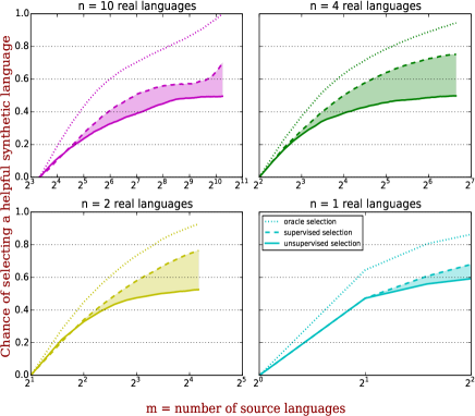
Figure 6: Chance that selecting a source from $m$ languages achieves strictly better dev UAS than just selecting from the $n$ real languages.

Figure 7 offers a fine-grained look at which real and synthetic source languages $S$ succeeded best when $T=\text{English}$. Each curve shows a different superstrate, with the $x$-axis ranging over substrates. (The figure omits the hundreds of synthetic source languages that use two distinct superstrates, $R_{\texttt{V}}\neq R_{\texttt{N}}$.) Real languages are shown as solid black dots, and are often beaten by synthetic languages. For comparison, this graph also plots results that “cheat” by using English supervision.

The above graphs are evaluated on development sentences in development languages. For our final results, Table 3, we finally allow ourselves to try transferring to the UD test languages, and we evaluate on test sentences. The comparison is similar to the comparison in the selection graph: do the synthetic treebanks add value? We use our largest source pools, $n=10$ and $m=1210$. With supervised selection, selecting the source language from the full pool of $m$ options (not just the $n$ real languages) tends to achieve significantly better UAS on the target language, often dramatically so. On average, the UAS on the test languages increases by 2.3 percentage points, and this increase is statistically significant across these 17 data points. Even with unsupervised selection, UAS still increases by 1.2 points on average, but this difference could be a chance effect.

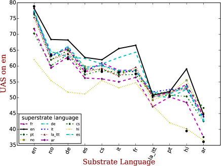
Figure 7: UAS performance of different source parsers when applied to English development sentences. The $x$ axis shows the 10 real training languages $S$, in decreasing order of their UAS performance (plotted as large black dots). For each superstrate $R$, we plot a curve showing—for each substrate $S$—the best UAS of the languages $S[R/{\texttt{N}}],S[R/{\texttt{V}}]$ and $S[R/{\texttt{N}},R/{\texttt{V}}]$. The points where $R=S$ are specially colored in black; these are instances of self-permutation (§5). We also add “cheating results” where English itself is used as the substrate (left column) and/or the superstrate (solid black line at top). Thus, the large black dot at the upper left is a supervised English parser.

	unsupervised		(weakly) supervised
target	real	+synthetic	real	+synthetic
el	60.07	65.72	65.87	66.98
he	63.39	60.65	62.86	64.28
la	46.79	51.82	56.62	59.06
hr	68.69	68.89	68.69	69.11
sv	74.96	74.96	74.96	74.96
hu	56.41	64.67	56.72	66.22
fa	53.41	58.37	53.41	60.18
fi_ftb	50.90	55.36	53.03	55.86
cu	54.11	57.89	54.11	59.28
ga	53.55	59.38	57.72	64.72
sl	80.41	80.41	80.41	80.41
eu	47.12	48.97	45.35	52.90
ro	66.33	68.01	71.38	69.19
ja_ktc	62.51	54.04	62.51	62.49
id	63.79	61.89	65.36	65.36
pl	75.69	74.63	75.69	73.05
ta	63.15	56.20	63.15	63.15
Test Avg.	61.25	62.46	62.81	65.13
bg	79.80	74.52	79.80	79.80
nl	58.44	57.94	58.44	57.85
et	68.83	72.21	68.83	74.75
la_proiel	48.50	49.66	48.50	49.66
da	71.65	71.65	71.65	70.79
en	63.37	61.37	63.37	65.43
grc	42.59	42.59	46.15	47.84
grc_proiel	50.76	51.29	52.04	54.06
fi	51.28	55.21	54.46	55.21
got	54.98	57.57	54.98	58.66
All Avg.	60.43	61.33	61.71	63.75

Table 3: Our final comparison on the 17 test languages appears in the upper part of this table. We ask whether single-source transfer to these 17 real target languages is improved by augmenting the source pool of 10 real languages with 1200 synthetic languages. When different languages are selected in these two settings, we boldface the setting with higher test UAS, or both settings if they are not significantly different (paired permutation test by sentence, $p<0.05$). For completeness, we extend the table with the 10 development languages. The “Avg.” lines report the average of 17 test or 27 test+dev languages. The two supervised-selection averages are significantly different (paired permutation test by language, $p<0.05$).

The results above use gold POS tag sequences for $T$. These may not be available if $T$ is a low-resource language; see Appendix B for a further experiment.

7.4 Discussion

Many of the curves in Figures 5–6 still seem to be increasing steadily at maximum $m$, which suggests that we would benefit from finding ways to generate even more synthetic languages. Diversity of languages seems to be crucial, since adding new real languages improves performance much faster than remixing existing languages. This suggests that we should explore making more extensive changes to the UD treebanks (see §8).

Surprisingly, Figures 5–6 show improvements even when $n=1$. Evidently, self-permutation of a single language introduces some useful variety, perhaps by transporting specialized word orders (e.g., English still allows some limited V2 constructions) into contexts where the source language would not ordinarily allow them but the target language does.

Figure 5 shows why unsupervised selection is considerably worse on average than supervised selection. Its 90th percentile is comparable, but at the 10th percentile—presumably representing experiments where no good sources are available—the unsupervised heuristic has more trouble at choosing among the mediocre options. The supervised method can actually test these options using the true loss function.

Figure 7 is interesting to inspect. English is essentially a Germanic language with French influence due to the Norman conquest, so it is reassuring that German and French substrates can each be improved by using the other as a superstrate. We also see that Arabic and Hindi are the worst source languages for English, but that Hindi[Arabic/V] is considerably better. This is because Hindi is reasonably similar to English once we correct its SOV word order to SVO (via almost any superstrate).

8 Conclusions and Future Work

This paper is the first release of a novel resource, the Galactic Dependencies treebank collection, that may unlock a wide variety of research opportunities (discussed in §1). Our empirical studies show that the synthetic languages in this collection remain somewhat natural while improving the diversity of the collection. As a simplistic but illustrative use of the resource, we carefully evaluated its impact on the naive technique of single-source transfer parsing. We found that performance could consistently be improved by adding synthetic languages to the pool of sources, assuming gold POS tags.

There are several non-trivial opportunities for improving and extending our treebank collection in future releases.

1. Our current method is fairly conservative, only synthesizing languages with word orders already attested in our small collection of real languages. This does not increase the diversity of the pool as much as when we add new real languages. Thus, we are particularly interested in generating a wider range of synthetic languages. We could condition reorderings on the surrounding tree structure, as noted in §3.2. We could choose reordering parameters ${\boldsymbol{\mathbf{\theta}}}_{X}$ more adventurously than by drawing them from a single known superstrate language. We could go beyond reordering, to systematically choose what function words (determiners, prepositions, particles), function morphemes, or punctuation symbols should appear in the synthetic tree, or to otherwise alter the structure of the tree Dorr (1993). These options may produce implausible languages. To mitigate this, we could filter or reweight our sample of synthetic languages—via rejection sampling or importance sampling—so that they are distributed more like real languages, as measured by their parsabilities, dependency lengths, and estimated WALS features Dryer and Haspelmath (2013).

2. Currently, our reordering method only generates projective dependency trees. We should extend it to allow non-projective trees as well—for example, by pseudo-projectivizing the substrate treebank Nivre and Nilsson (2005) and then deprojectivizing it after reordering.

3. The treebanks of real languages can typically be augmented with larger unannotated corpora in those languages Majliš (2011), which can be used to train word embeddings and language models, and can also be used for self-training and bootstrapping methods. We plan to release comparable unannotated corpora for our synthetic languages, by automatically parsing and permuting the unnanotated corpora of their substrate languages.

4. At present, all languages derived from an English substrate use the English vocabulary. In the future, we plan to encipher that vocabulary separately for each synthetic language, perhaps choosing a cipher so that the result loosely conforms to the realistic phonotactics and/or orthography of some superstrate language. This would let multilingual methods exploit lexical features without danger of overfitting to specific lexical items that appear in many synthetic training languages. Alphabetic ciphers can preserve features of words that are potentially informative for linguistic structure discovery: their cooccurrence statistics, their length and phonological shape, and the sharing of substrings among morphologically related words.

5. Finally, we note that this paper has focused on generating a broadly reusable collection of synthetic treebanks. For some applications (including single-source transfer), one might wish to tailor a synthetic language on demand, e.g., starting with one of our treebanks but modifying it further to more closely match the surface statistics of a given target language Dorr et al. (2002). In our setup, this would involve actively searching the space of reordering parameters, using algorithms such as gradient ascent or simulated annealing.

We conclude by revisiting our opening point. Unsupervised discovery of linguistic structure is difficult. We often do not know quite what function to maximize, or how to globally maximize it. If we could make labeled languages as plentiful as labeled images, then we could treat linguistic structure discovery as a problem of supervised prediction—one that need not succeed on all formal languages, but which should generalize at least to the domain of possible human languages.

Appendix A Constructing the Kite Graph

The mean lines in the “kite graph” (Figure 5) are actually obtained by averaging 10,000 graphs. Each of these graphs is “smooth” because it incrementally adds new languages as $n$ or $m$ increases. Pseudocode to generate one such graph is given as Algorithm 1; all random choices are made uniformly.

Algorithm 1 Data collection for one graph

1:Sets ${\cal T}$ (target languages), ${\cal S}$ (real source languages), ${\cal S}^{\prime}$ (synthetic source languages)

2:Sets of data points $D_{\text{sup}}$, $D_{\text{unsup}}$

3:procedure CollectData

4:    $D\leftarrow\varnothing$

5:    Sample a target language $T$ from $\cal T$

6:    $L\leftarrow\text{random.shuffle}(\mathcal{S}-\{T\})$

7:    $L^{\prime}\leftarrow\text{random.shuffle}(\mathcal{S^{\prime}})$

8:    for $n=1$ to $|L|$ do

9:         $L^{\prime\prime}\leftarrow{}$ a filtered version of $L^{\prime}$ that excludes languages with substrates or superstrates outside $\{L_{1},\ldots,L_{n}\}$

10:         for $n^{\prime}=1$ to $|L^{\prime\prime}|$ do

11:             ${\cal P}\leftarrow\{L_{1},\ldots,L_{n},L^{\prime\prime}_{1},\ldots,L^{\prime\prime}_{n^{\prime}}\}$

12:             $m\leftarrow|{\cal P}|$

13:             $D_{\text{sup}}\leftarrow{}$ $D_{\text{sup}}\cup\\ \{(n,m,\textsc{uas}_{\text{sup}}({\cal P},T))\}$

14:             $D_{\text{unsup}}\leftarrow{}$ $D_{\text{unsup}}\cup\\ \{(n,m,\textsc{uas}_{\text{unsup}}({\cal P},T))\}$              

15:    return $(D_{\text{sup}}$, $D_{\text{unsup}})$

Appendix B Experiment with Noisy Tags

Table 4 repeats the single-source transfer experiment using noisy automatic POS tags for $T$ for both parser input and unsupervised selection. We obtained the tags using RDRPOSTagger Nguyen et al. (2014) trained on just 100 gold-tagged sentences (the same set used for supervised selection). The low tagging accuracy does considerably degrade UAS and muddies the usefulness of the synthetic sources.

	tag	unsupervised		(weakly) superv.
target		real	+synth	real	+synth
bg	78.33	53.24	55.08	53.24	53.24
nl	71.70	39.40	38.99	42.42	42.75
et	72.88	45.19	54.81	56.07	55.09
la_proiel	71.83	37.25	38.26	37.25	38.10
da	78.04	47.98	43.40	47.98	45.89
en	77.33	48.29	44.40	48.29	48.15
grc	68.80	32.15	32.15	33.52	34.36
grc_proiel	72.93	42.46	41.39	43.49	44.19
fi	65.65	29.59	28.81	36.85	36.90
got	76.66	44.77	44.05	44.77	46.83
Avg.	73.42	42.03	42.13	44.39	44.55

Table 4: Tagging accuracy on the 10 dev languages, and UAS of the selected source parser with these noisy target-language tag sequences. The results are formatted as in Table 3, but here all results are on dev sentences.

Acknowledgements

This work was funded by the U.S. National Science Foundation under Grant No. 1423276. Our data release is derived from the Universal Dependencies project, whose many selfless contributors have our gratitude. We would also like to thank Matt Gormley and Sharon Li for early discussions and code prototypes, Mohammad Sadegh Rasooli for guidance on working with the Yara parser, and Jiang Guo, Tim Vieira, Adam Teichert, and Nathaniel Filardo for additional useful discussion. Finally, we thank TACL editors Joakim Nivre and Lillian Lee and the anonymous reviewers for several suggestions that improved the paper.

References

- Abu-Mostafa (1995) Yaser S. Abu-Mostafa. Hints. Neural Computation, 7:639–671, July 1995.
- Borg and Groenen (2005) Ingwer Borg and Patrick J.F. Groenen. Modern Multidimensional Scaling: Theory and Applications. 2005.
- Chomsky (1981) Noam Chomsky. Lectures on Government and Binding: The Pisa Lectures. Holland: Foris Publications, 1981.
- Collins et al. (2005) Michael Collins, Philipp Koehn, and Ivona Kucerova. Clause restructuring for statistical machine translation. In Proceedings of the 43rd Annual Meeting of the Association for Computational Linguistics, pages 531–540, 2005.
- Cotterell et al. (2015) Ryan Cotterell, Nanyun Peng, and Jason Eisner. Modeling word forms using latent underlying morphs and phonology. Transactions of the Association for Computational Linguistics, 3:433–447, 2015.
- Cui et al. (2015) Xiaodong Cui, Vaibhava Goel, and Brian Kingsbury. Data augmentation for deep neural network acoustic modeling. IEEE/ACM Transactions on Audio, Speech and Language Processing, 23(9):1469–1477, September 2015. ISSN 2329-9290.
- Dorr (1993) Bonnie J. Dorr. Machine Translation: A View from the Lexicon. MIT Press, Cambridge, MA, 1993.
- Dorr et al. (2002) Bonnie J. Dorr, Lisa Pearl, Rebecca Hwa, and Nizar Habash. DUSTer: A method for unraveling cross-language divergences for statistical word-level alignment. In Proceedings of the 5th Conference of the Association for Machine Translation in the Americas on Machine Translation: From Research to Real Users, AMTA ’02, pages 31–43, 2002.
- Dryer and Haspelmath (2013) Matthew S. Dryer and Martin Haspelmath, editors. The World Atlas of Language Structures Online. Max Planck Institute for Evolutionary Anthropology, Leipzig, 2013.
- Duong et al. (2015) Long Duong, Trevor Cohn, Steven Bird, and Paul Cook. Cross-lingual transfer for unsupervised dependency parsing without parallel data. In Proceedings of the 19th Conference on Computational Natural Language Learning, pages 113–122, 2015.
- Eisner and Smith (2010) Jason Eisner and Noah A. Smith. Favor short dependencies: Parsing with soft and hard constraints on dependency length. In Harry Bunt, Paola Merlo, and Joakim Nivre, editors, Trends in Parsing Technology: Dependency Parsing, Domain Adaptation, and Deep Parsing, chapter 8, pages 121–150. 2010.
- Ganchev et al. (2010) Kuzman Ganchev, Joao Graça, Jennifer Gillenwater, and Ben Taskar. Posterior regularization for structured latent variable models. Journal of Machine Learning Research, 11:2001–2049, 2010.
- Guo et al. (2015) Jiang Guo, Wanxiang Che, David Yarowsky, Haifeng Wang, and Ting Liu. Cross-lingual dependency parsing based on distributed representations. In Proceedings of the 53rd Annual Meeting of the Association for Computational Linguistics and the 7th International Joint Conference on Natural Language Processing, pages 1234–1244, 2015.
- Hawkins (1994) John Hawkins. A Performance Theory of Order and Constituency. Cambridge University Press, 1994.
- Hermann et al. (2015) Karl Moritz Hermann, Tomas Kocisky, Edward Grefenstette, Lasse Espeholt, Will Kay, Mustafa Suleyman, and Phil Blunsom. Teaching machines to read and comprehend. In Advances in Neural Information Processing Systems, pages 1684–1692, 2015.
- Howlett and Dras (2011) Susan Howlett and Mark Dras. Clause restructuring for SMT not absolutely helpful. In Proceedings of the 49th Annual Meeting of the Association for Computational Linguistics: Human Language Technologies, pages 384–388, 2011. Erratum at https://www.aclweb.org/anthology/P/P11/P11-2067e1.pdf.
- Jaitly and Hinton (2013) Navdeep Jaitly and Geoffrey E. Hinton. Vocal tract length perturbation (VTLP) improves speech recognition. In Proceedings of the 30th International Conference on Machine Learning Workshop on Deep Learning for Audio, Speech and Language, 2013.
- Klein and Manning (2004) Dan Klein and Christopher Manning. Corpus-based induction of syntactic structure: Models of dependency and constituency. In Proceedings of the 42nd Annual Meeting of the Association for Computational Linguistics, pages 478–485, 2004.
- Krizhevsky et al. (2012) Alex Krizhevsky, Ilya Sutskever, and Geoffrey E. Hinton. ImageNet classification with deep convolutional neural networks. In F. Pereira, C.J.C. Burges, L. Bottou, and K.Q. Weinberger, editors, Advances in Neural Information Processing Systems 25, pages 1097–1105. 2012.
- Ma and Xia (2014) Xuezhe Ma and Fei Xia. Unsupervised dependency parsing with transferring distribution via parallel guidance and entropy regularization. In Proceedings of the 52nd Annual Meeting of the Association for Computational Linguistics, volume 1, pages 1337–1348, 2014.
- Majliš (2011) Martin Majliš. W2C—web to corpus—corpora, 2011. LINDAT/CLARIN digital library at the Institute of Formal and Applied Linguistics, Charles University in Prague.
- McDonald et al. (2011) Ryan McDonald, Slav Petrov, and Keith Hall. Multi-source transfer of delexicalized dependency parsers. In Proceedings of the 2011 Conference on Empirical Methods in Natural Language Processing, pages 62–72, 2011.
- Naseem et al. (2010) Tahira Naseem, Harr Chen, Regina Barzilay, and Mark Johnson. Using universal linguistic knowledge to guide grammar induction. In Proceedings of the 2010 Conference on Empirical Methods in Natural Language Processing, pages 1234–1244, 2010.
- Nguyen et al. (2014) Dat Quoc Nguyen, Dai Quoc Nguyen, Dang Duc Pham, and Son Bao Pham. RDRPOSTagger: A ripple down rules-based part-of-speech tagger. In Proceedings of the Demonstrations at the 14th Conference of the European Chapter of the Association for Computational Linguistics, pages 17–20, 2014.
- Nivre and Nilsson (2005) Joakim Nivre and Jens Nilsson. Pseudo-projective dependency parsing. In Proceedings of the 43rd Annual Meeting of the Association for Computational Linguistics, pages 99–106, 2005.
- Nivre et al. (2015) Joakim Nivre, Željko Agić, Maria Jesus Aranzabe, Masayuki Asahara, Aitziber Atutxa, Miguel Ballesteros, John Bauer, Kepa Bengoetxea, Riyaz Ahmad Bhat, Cristina Bosco, Sam Bowman, Giuseppe G. A. Celano, Miriam Connor, Marie-Catherine de Marneffe, Arantza Diaz de Ilarraza, Kaja Dobrovoljc, Timothy Dozat, Tomaž Erjavec, Richárd Farkas, Jennifer Foster, Daniel Galbraith, Filip Ginter, Iakes Goenaga, Koldo Gojenola, Yoav Goldberg, Berta Gonzales, Bruno Guillaume, Jan Hajič, Dag Haug, Radu Ion, Elena Irimia, Anders Johannsen, Hiroshi Kanayama, Jenna Kanerva, Simon Krek, Veronika Laippala, Alessandro Lenci, Nikola Ljubešić, Teresa Lynn, Christopher Manning, Cătălina Mărănduc, David Mareček, Héctor Martínez Alonso, Jan Mašek, Yuji Matsumoto, Ryan McDonald, Anna Missilä, Verginica Mititelu, Yusuke Miyao, Simonetta Montemagni, Shunsuke Mori, Hanna Nurmi, Petya Osenova, Lilja Øvrelid, Elena Pascual, Marco Passarotti, Cenel-Augusto Perez, Slav Petrov, Jussi Piitulainen, Barbara Plank, Martin Popel, Prokopis Prokopidis, Sampo Pyysalo, Loganathan Ramasamy, Rudolf Rosa, Shadi Saleh, Sebastian Schuster, Wolfgang Seeker, Mojgan Seraji, Natalia Silveira, Maria Simi, Radu Simionescu, Katalin Simkó, Kiril Simov, Aaron Smith, Jan Štěpánek, Alane Suhr, Zsolt Szántó, Takaaki Tanaka, Reut Tsarfaty, Sumire Uematsu, Larraitz Uria, Viktor Varga, Veronika Vincze, Zdeněk Žabokrtský, Daniel Zeman, and Hanzhi Zhu. Universal dependencies 1.2, 2015. LINDAT/CLARIN digital library at the Institute of Formal and Applied Linguistics, Charles University in Prague.
- Nivre et al. (2016) Joakim Nivre, Marie-Catherine de Marneffe, Filip Ginter, Yoav Goldberg, Jan Hajič, Christopher Manning, Ryan McDonald, Slav Petrov, Sampo Pyysalo, Natalia Silveira, Reut Tsarfaty, and Daniel Zeman. Universal dependencies v1: A multilingual treebank collection. In Proceedings of the 10th International Conference on Language Resources and Evaluation, pages 1659–1666, 2016.
- Nunberg (1990) Geoffrey Nunberg. The Linguistics of Punctuation. Number 18 in CSLI Lecture Notes. Center for the Study of Language and Information, 1990.
- Rasooli and Collins (2015) Mohammad Sadegh Rasooli and Michael Collins. Density-driven cross-lingual transfer of dependency parsers. In Proceedings of the 2015 Conference on Empirical Methods in Natural Language Processing, pages 328–338, 2015.
- Rasooli and Tetreault (2015) Mohammad Sadegh Rasooli and Joel R. Tetreault. Yara parser: A fast and accurate dependency parser. Computing Research Repository, arXiv:1503.06733 (version 2), 2015.
- Rasooli et al. (2014) Mohammad Sadegh Rasooli, Thomas Lippincott, Nizar Habash, and Owen Rambow. Unsupervised morphology-based vocabulary expansion. In Proceedings of the 52nd Annual Meeting of the Association for Computational Linguistics (Volume 1: Long Papers), pages 1349–1359, June 2014.
- Rozovskaya and Roth (2010) Alla Rozovskaya and Dan Roth. Training paradigms for correcting errors in grammar and usage. In Human Language Technologies: The 2010 Annual Conference of the North American Chapter of the Association for Computational Linguistics, pages 154–162, 2010.
- Sedgewick (1977) Robert Sedgewick. Permutation generation methods. ACM Computing Surveys, 9(2):137–164, 1977.
- Serban et al. (2016) Iulian Vlad Serban, Alberto García-Durán, Caglar Gulcehre, Sungjin Ahn, Sarath Chandar, Aaron Courville, and Yoshua Bengio. Generating factoid questions with recurrent neural networks: The 30m factoid question-answer corpus. In Proceedings of the 54th Annual Meeting of the Association for Computational Linguistics (Volume 1: Long Papers), pages 588–598. Association for Computational Linguistics, 2016.
- Simard et al. (2003) Patrice Y. Simard, Dave Steinkraus, and John C. Platt. Best practices for convolutional neural networks applied to visual document analysis. In Proceedings of the 7th International Conference on Document Analysis and Recognition, pages 958–, 2003.
- Smith and Eisner (2006) Noah A. Smith and Jason Eisner. Annealing structural bias in multilingual weighted grammar induction. In Proceedings of the 21st International Conference on Computational Linguistics and 44th Annual Meeting of the Association for Computational Linguistics, pages 569–576, 2006.
- Søgaard (2011) Anders Søgaard. Data point selection for cross-language adaptation of dependency parsers. In Proceedings of the 49th Annual Meeting of the Association for Computational Linguistics: Human Language Technologies, pages 682–686, 2011.
- Spitkovsky (2013) Valentin I. Spitkovsky. Grammar Induction and Parsing with Dependency-and-Boundary Models. PhD thesis, Computer Science Department, Stanford University, Stanford, CA, 2013.
- Spitkovsky et al. (2013) Valentin I. Spitkovsky, Hiyan Alshawi, and Daniel Jurafsky. Breaking out of local optima with count transforms and model recombination: A study in grammar induction. In Proceedings of the 2013 Conference on Empirical Methods in Natural Language Processing, pages 1983–1995, 2013.
- Varjokallio and Klakow (2016) Matti Varjokallio and Dietrich Klakow. Unsupervised morph segmentation and statistical language models for vocabulary expansion. In Proceedings of the 54th Annual Meeting of the Association for Computational Linguistics (Volume 2: Short Papers), pages 175–180, 2016.
- Vilares et al. (2011) Jesús Vilares, Manuel Vilares, and Juan Otero. Managing misspelled queries in IR applications. Information Processing & Management, 47(2):263–286, 2011.
- Wang et al. (2015) Yushi Wang, Jonathan Berant, and Percy Liang. Building a semantic parser overnight. In Proceedings of the 53rd Annual Meeting of the Association for Computational Linguistics and the 7th International Joint Conference on Natural Language Processing (Volume 1: Long Papers), pages 1332–1342, 2015.
- Weston et al. (2016) Jason Weston, Antoine Bordes, Sumit Chopra, and Tomas Mikolov. Towards AI-complete question answering: A set of prerequisite toy tasks. In Proceedings of the International Conference on Learning Representations, 2016.