DeBroglie-Bohm interpretation of a Hořava-Lifshitz quantum cosmology model
Abstract
In the present letter, we consider the DeBroglie-Bohm interpretation of a Hořava-Lifshitz quantum cosmology model in the presence of a radiation perfect fluid. We compute the Bohm’s trajectories for the scale factor and show that it never goes to zero. That result gives a strong indication that this model is free from singularities, at the quantum level. We also compute the quantum potential. That quantity helps understanding why the scale factor never vanishes.
Any quantized theory of the gravitational interaction when applied to cosmology will face an important problem related to its interpretation. The well established Copenhagen interpretation of quantum mechanics cannot be applied to such theories because it is not possible to apply a statistical interpretation to a system composed of the entire Universe. One cannot repeat the experiments for that system. A very interesting interpretation of quantum mechanics, which in many aspects leads to the same results as the Copenhagen interpretation and can be applied to a system composed of the entire Universe is the DeBroglie-Bohm interpretation of quantum mechanics [1], [2]. That interpretation has been applied to several models of quantum cosmology with great success [3], [4], [5], [6], [7]. In most of those models, the authors compute the scale factor trajectory and shows that this quantity never vanishes. That result gives a strong indication that those models are free from singularities, at the quantum level. Another important quantity introduced by the DeBroglie-Bohm interpretation is the quantum potential () [1], [2]. For those quantum cosmology models, the determination of helps understanding why the scale factor never vanishes.
Some years ago a very interesting geometrical theory of gravity was introduced [8]. That theory, now called Hořava-Lifstz (HL), has an explicit asymmetry between space and time, which manifests through an anisotropic scaling between space and time. That property means that the Lorentz symmetry is broken, at least at high energies, where that asymmetry between space and time takes place. At low energies the HL theory tends to General Relativity (GR), recovering the Lorentz symmetry. Due to the asymmetry between space and time present in his geometrical theory of gravity, Hořava decided to formulate it using the Arnowitt-Deser-Misner (ADM) formalism, which splits the four dimensional spacetime in a time line plus three dimensional space [13]. In the ADM formalism the four dimensional metric () is decomposed in terms of the three dimensional metric (), of spatial sections, the shift vector and the lapse function . In general all those quantities depend on space and time. In his original work, Hořava considered the simplified assumption that should depend only on time [8]. This assumption became known as the projectable condition. The gravitational action of the HL theory was proposed such that the kinetic component was constructed separately from the potential one. The kinetic component was motivated by the one coming from general relativity, written in terms of the extrinsic curvature tensor. The potential component must depend only on the spatial metric and its spatial derivatives. As a geometrical theory of gravity the potential component of the HL theory should be composed of scalar contractions of the Riemann tensor and its spatial derivatives. In his original paper [8], Hořava considered a simplification in order to reduce the number of possible terms contributing to the potential component of his theory. It is called the detailed balance condition. The HL theory have been applied to cosmology and produced very interesting models [9], [10], [11], [12].
In the present letter, we consider the DeBroglie-Bohm interpretation of a Hořava-Lifshitz quantum cosmology model in the presence of a radiation perfect fluid. The model have already been studied in Ref. [11]. There, the authors solved the corresponding Wheeler-DeWitt equation, found the wavefunction and computed an approximate value of the scale factor expected value. Here, we compute the exact scale factor expected value and the Bohm’s trajectories for the scale factor of that model and show that they never go to zero. That result gives a strong indication that the model is free from singularities, at the quantum level. We also compare that trajectory with the scale factor expected value. Finally, we compute the quantum potential for that model. That quantity helps understanding why the scale factor never vanishes.
Following the authors of Ref. [11], we study, here, Friedmann-Robertson-Walker quantum cosmology models in the framework of a projectable HL gravity without detailed balance condition. The matter content of the models is a perfect fluid with equation of state: , where is the fluid pressure and its energy density. The constant curvature of the spatial sections may be positive (), negative () or zero (). The model may be written in its Hamiltonian form with the aid of the ADM formalism [13] and the Schutz’s variational formalism [14], [15]. The authors of Ref. [11] did that and found the following total hamiltonian,
| (1) |
The phase space of those models are described by the scale factor , a variable associated to the fluid and their canonically conjugated momenta and , respectively. All of them are functions only of the time coordinate . The coefficients , , and , are coupling constants introduced by the Hořava-Lifshitz theory [16]. The authors of Ref. [11], restricted their attention to the gauge .
The quantum version of the theory is obtained by replacing the moments by their corresponding operator expressions and the application of the resulting total hamiltonian operator to a wavefunction . The resulting equation is the Wheeler-DeWitt equation. For the present model it is given by [11],
| (2) |
where is a parameter that accounts for the ambiguity in the ordering of factors and in the first term of eq. (1). The authors of Ref. [11], restricted their attention to the case . Now, we perform the following separation of variables in ,
| (3) |
Introducing Eq. (3) in eq. (2), we find the following equation for ,
| (4) |
For , the authors of Ref. [11], found exact solutions to a simplified version of eq. (4), obtained by setting . The motivation for doing that simplification is the fact that one may neglect the terms with those coefficients at the beginning of the Universe. In particular, let us study the solution to the model with radiation () using the DeBroglie-Bohm interpretation.
Solution for and
For the present case, the authors of Ref. [11] found the following solution to a simplified version of eq. (4), obtained by setting ,
| (5) |
where is the Bessel function of the first kind. Now, introducing in eq. (3), it is possible to construct a wave-packet out of the resulting expression. In order to do that, one has to integrate, the resulting expression, over , from 0 to , with an appropriate weight function. The authors of Ref. [11] did that and found the following wave-packet,
| (6) |
where is a small positive constant. For simplicity let us choose . We want, now, to write eq. (6) in its polar form,
| (7) |
After some calculation, we obtain,
From eq. (Solution for and ), we may identify and as,
| (9) | |||||
| (10) |
From eq. (Solution for and ), it is possible to compute the scale factor expected value, using the expression,
| (11) |
Therefore, introducing eq. (Solution for and ) in eq. (11), we obtain the following exact expression for the scale factor expected value,
| (12) |
The authors of Ref. [11] found an approximate expression for the scale factor expected value.
Now, we want to describe that model in the DeBroglie-Bohm interpretation. In that interpretation, we may compute the scale factor trajectory using the following equation [2],
| (13) |
where is the phase, eq. (10), of , eq. (Solution for and ). From Ref. [11], we have that,
| (14) |
In the gauge , for the present case of radiation where , and eq. (14), we may write eq. (13) as,
| (15) |
Introducing the phase eq. (10) in eq. (15) and performing the partial derivative and integration indicated, we obtain the following scale factor trajectory,
| (16) |
where is the initial value of and is the value of . Comparing the scale factor expected value eq. (12) and its DeBroglie-Bohm trajectory eq. (16), we notice that those expressions depend on in the same way. If we fix and
| (17) |
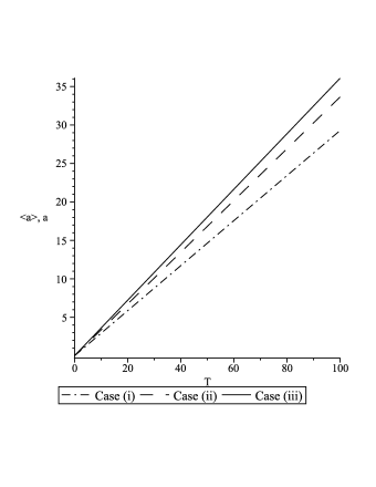
both scale factor expected value eq. (12) and its DeBroglie-Bohm trajectory eq. (16) are the same. That trajectory eq. (16), represents an universe that starts, at , from a minimum size eq. (17) and expands to an infinity size, as , when . Therefore, it is free from singularities at the quantum level. Observing the expressions of eq. (12) or eq. (16), which are the same for given by eq. (17), we notice that they depend on two parameters: and . After a detailed numerical study on how or depend on those parameters, we reached the following conclusions. Since and always appear together, as , in the expressions of or , we have three different cases: (i) , (ii) and (iii) . It is important to notice that for case (i) or will be real-valued only if the condition is satisfied. That restriction, in the values of the parameter , for case (i), shows the limitations of the present simplification used in order to obtain solution (5). We hope, in a future work, solving the complete equation (4). If one fixes the value of such that have the same absolute value, for cases (i) and (iii), one obtains that or always have the greater and expand more rapidly for case (iii), next for case (ii) and finally for case (i). Those results are in agreement to the corresponding classical model [11]. An example comparing the scale factor expected values or the DeBroglie-Bohm trajectories for those three cases is shown in Figure 1.
Using the quantum potential it is possible to understand why the scale factor trajectory eq. (16) does not go to zero when . In order to obtain the quantum potential , first we introduce the polar form of the wave function eq. (7) in the Wheeler-DeWitt equation (2), for the radiation perfect fluid () and the factor ordering ambiguities parameter . It will produce two equations: a real one and a purely imaginary one. The real equation is given by,
| (18) |
where the quantum potential is,
| (19) |
The second part of the expression of , comes from the choice of taking in account factor order ambiguities [17], [18]. For the simplified version of the Wheeler-DeWitt equation considered, in order to obtain the solution eq. (5), the classical potential is,
| (20) |
In order to compute , we introduce eq. (9) in eq. (19) and obtain the following expression,
| (21) |
Now, we have to evaluate the quantum potential eq. (21) over the DeBroglie-Bohm trajectory eq. (16) with given by eq. (17) and setting . We may write the quantum potential as a function of (),
| (22) |
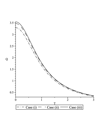
After a detailed numerical study of eq. (22), we find that for the three cases considered above: (i) , (ii) and (iii) , is positive and finite at , then it decreases as increases and asymptotically it goes to zero when , for all possible values of (depending on each case). An example of the quantum potential, over the DeBroglie-Bohm trajectory Q(T), for the three situations described in the text is shown in Figure 2. It is interesting to notice that, for case (i) , observing the classical potential eq. (20), we notice that gives rise to a potential well when . The effective potential, which is given by the sum of eq. (20) with eq. (22), is positive and finite at , then it decreases as increases and asymptotically it goes to zero when , for all possible values of . For case (ii) , the classical potential eq. (20) is zero. For that case, the model becomes similar to the corresponding one in quantum cosmology based on general relativity coupled to a radiation perfect fluid. The DeBroglie-Bohm interpretation of that model has already been treated in Ref. [19] and their results are in agreement with ours. For case (iii) , observing the classical potential eq. (20), we notice that , along with , also produces a potential barrier that prevents the value of the scale factor ever to go through zero, at . Therefore, for the three cases there will be a potential barrier, at , that prevents the value of the scale factor ever to go through zero.
Acknowledgements. L. G. Martins thanks CAPES for her scholarship. G. A. Monerat thanks UERJ for the Prociência grant, via FAPERJ.
References
- [1] D. Bohm and B. J. Hiley, The undivided universe: an ontological interpretation of quantum theory, Routledge, London, 1993;
- [2] P. R. Holland, The quantum theory of motion: an account of the de Broglie-Bohm interpretation of quantum mechanics, Cambridge University Press, Cambridge, 1993.
- [3] J. Acacio de Barros, N. Pinto-Neto and M. A. Sagioro-Leal, Phys. Lett. A 241 (1998) 229.
- [4] G. D. Barbosa and N. Pinto-Neto, Phys. Rev. D 70, 103512 (2004).
- [5] G. D. Barbosa, Phys. Rev. D 71, 063511 (2005).
- [6] G. Oliveira-Neto, E. V. Corrêa Silva, N. A. Lemos, G. A. Monerat, Phys. Lett. A 373, 2012 (2009).
- [7] G. Oliveira-Neto, M. Silva de Oliveira, G. A. Monerat and E. V. Corrêa Silva, Int. J. Mod. Phys. D 26, 1750011 (2016).
- [8] P. Hořava, Phys. Rev. D 79, 084008 (2009).
- [9] O. Bertolami and C. A. D. Zarro, Phys. Rev. D 84, 044042 (2011).
- [10] B. C. Paul, P. Thakur and A. Saha, Phys. Rev. D 85, 024039 (2012).
- [11] B. Vakili and V. Kord, Gen. Relativ. Gravit. 45, 1313 (2013).
- [12] H. Ardehali and P. Pedram, Phys. Rev. D 93, 043532 (2016).
- [13] R. Arnowitt, S. Deser and C. W. Misner, in Gravitation: an introduction to current research, ed. L. Witten (Wiley, New York, 1962), Chapter 7, pp 227-264 and arXiv:gr-qc/0405109.
- [14] Schutz, B. F., Phys. Rev. D 2, 2762, (1970).
- [15] Schutz, B. F., Phys. Rev. D 4, 3559, (1971).
- [16] K. Maeda, Y. Misonoh and T. Kobayashi, Phys. Rev. D 82, 064024 (2010).
- [17] R. Colistete, Jr., J. C. Fabris and N. Pinto-Neto, Phys. Rev. D 57, 4707 (1998).
- [18] H. Dongshan, G. Dongfeng and C. Qing-yu, Phys. Rev. D 89, 083510 (2014).
- [19] F.G. Alvarenga, J.C. Fabris, N.A. Lemos and G.A. Monerat, Gen. Rel. Grav. 34, 651 (2002).