Radiative Neutrino Mass & Majorana Dark Matter within an Inert Higgs Doublet Model

Abstract

We consider an extension of the standard model (SM) with an inert Higgs doublet and three Majorana singlet fermions to address both origin and the smallness of neutrino masses and dark matter (DM) problems. In this setup, the lightest Majorana singlet fermion plays the role of DM candidate and the model parameter space can be accommodated to avoid different experimental constraints such as lepton flavor violating processes and electroweak precision tests. The neutrino mass is generated at one-loop level a la Scotogenic model and its smallness is ensured by the degeneracy between the CP-odd and CP-even scalar members of the inert doublet. Interesting signatures at both leptonic and hadronic colliders are discussed.

I Introduction

The Discovery of the Higgs particle at the LHC in 2012 Aad:2012tfa , validated the standard model (SM) of particle physics. Although the SM has been very successful in describing and explaining the non-gravitational fundamental interactions between elementary particles, there are still open questions that it does not answer. For instance, the observation of neutrino oscillations in solar, atmospheric, reactor and accelerator experiments confirmed that neutrino have tiny non zero mass, unlike in the SM where they are strictly massless. Another issue that the SM does not account for is the existence of dark matter (DM) inferred from different astronomical and cosmological observations. Thus, going beyond the SM seems to be necessary in order to address these problems.

The most popular mechanism for explaining the smallness of neutrino mass is the see-saw mechanism, where a massive right handed neutrino (RHN) couples to the lepton and the Higgs doublets fields, and which at low energies induces the effective dimension five operator

$${\cal L}_{\text{eff}}^{(5)}=\frac{\kappa_{ij}}{\Lambda}~{}(\bar{L_{i}^{c}}~{}i\sigma_{2}~{}H)(L_{j}^{T}~{}i\sigma_{2}~{}H)+h.c,$$ (1)

where $\Lambda$ is the scale of new physics which is of order the RH neutrino mass, $\kappa_{ij}$ is a product of Yukawa couplings, $L$ and $L^{c}$ are the Lepton $SU(2)_{L}$ doublet and its charge conjugate, respectively, and $H$ is the Higgs doublet. However, on the basis of naturalness, the scale $\Lambda$ needs to be of order the GUT scale, making it impossible to probe it in high energy laboratory experiments. One way to lower the scale of the new physics is by generating neutrino masses radiatively where their smallness can be naturally explained by the loop suppression factor(s) and the Yukawa couplings. This can be realized at one loop Zee:1985rj , two loops Zee-86 , three loops Aoki:2008av ; knt , or four loops Nomura:2016fzs . In knt3 it has been shown that there is a class of three loop neutrino mass generation models, where the new particles that enter in the neutrino loop can be promoted to triplets knt3 , quintuplet knt5 , septuplets knt7 , and within a scale-invariant framework Ahriche:2015loa . An interesting features of these class of models is that the scale of new physics can be of order TeV, making them testable at high energy colliders hna ; Cheung:2004xm (For a review, see Cai:2017jrq ). Moreover, the electroweak phase transition can be strongly first order, an essential ingredient for successful electroweak baryogenesis EWPhT .

One of the simplest extensions of the scalar sector of the SM is the inert Higgs doublet model (IHDM) where one add an extra scalar doublet, $\Phi$, and assumes that there is a discrete $Z_{2}$ symmetry under which $\Phi$ is odd whereas the SM fields are even  Deshpande:1977rw . The Phenomenology of the (IHDM) has been studied extensively in the literature Gustafsson:2007pc . The discrete symmetry $Z_{2}$ has the following features: i) absence of the flavor changing neutral currents at tree level Glashow:1976nt , ii) the scalar of the inert doublet does not have interactions with active fermions and therefore its neutral component, denoted by $H^{0}$, can be a good candidate for DM. It has been shown that if $H^{0}$ is lighter than about $\leq 50\textrm{ GeV}$, the null results from DM direct detection experiment implies that annihilation cross section of the neutral inert scalar into SM light fermions is highly suppressed, giving too large relic density to what is observed by Planck experiment . In the mass range $140\textrm{ GeV}<m_{H^{0}}\leq 550\textrm{GeV}$, the annihilation into $W^{+}W^{-}$ is too large, rendering the relic density too small to be compatible with the astrophysical observations. There are three mass regions where the inert scalar can be a viable DM candidate: i) $m_{H^{0}}\simeq m_{h}/2$, with $m_{h}$ is the SM Higgs mass, corresponding to the annihilation via the s-channel resonance due to Higgs exchange Borah:2017dqx , ii) $m_{H^{0}}$ around the mass of the $W$ gauge boson, where the annihilation is into the three-body final state $WW^{*}\rightarrow Wff^{\prime}$  Honorez:2010re , and iii) $m_{H^{0}}\sim~{}\text{TeV}$ with scalar couplings of order unity Choubey:2017hsq . One possible way to produce the correct relic density and not being in conflict with DM direct detection experiment is by extending this model with heavy $SU(2)_{L}$ singlet vector-like charged leptons Borah:2017dqx .

In the present work, we consider the SM extended by an inert doublet and three RHNs Ma:2006km in order to address both neutrino mass and DM problem. We will investigate the case where the lightest Majorana singlet fermion plays the role of DM candidate instead of the neutral CP-odd or CP-even scalars. We will show that the model parameter space can be accommodated to avoid different experimental constraints such as lepton flavor violating processes and electroweak precision tests. In this setup, the neutrino mass smallness is ensured by making the splitting between the CP-even and CP-odd scalars very tiny. We will study different phenomenological aspects of the model and investigate the different regions of the parameter space that fulfill various theoretical and experimental constraints. In addition, we discuss the signatures for probing the model at both leptonic and hadronic colliders are discussed.

The paper is organized as follows; in section II, we highlight the model, its parameters and the different constraints under which the model is subject to. In section III, we present some selected results. In section IV, we discuss briefly the possible signatures of this model at hadronic and leptonic collider machines. In section V, we give our conclusion.

II The Model: Parameters and Constraints

II.1 The Model and Mass Spectrum

Here we consider the extension of the SM with an inert doublet $\Phi$ and three singlet Majorana fermions $N_{i}\sim(1,1,0)$, $i=1,2,3$, both odd under a discrete $Z_{2}$ symmetry. The relevant terms for generating neutrino mass at one loop are

$$\mathcal{L} \supset h_{ij}\bar{L}_{i}\epsilon\Phi N_{j}+\frac{1}{2}M_{i}\bar{N}_{i}^{C}N_{i}+h.c.,$$ (2)

where $\bar{L}_{i}$ is the left-handed lepton doublet and $\epsilon=i\sigma_{2}$ is an antisymmetric tensor. The scalar potential can be written as

$$V = -\mu_{1}^{2}|H|^{2}+\mu_{2}^{2}|\Phi|^{2}+\frac{\lambda_{1}}{6}|H|^{4}+\frac{\lambda_{2}}{6}|\Phi|^{4}+\lambda_{3}|H|^{2}|\Phi|^{2}+\frac{\lambda_{4}}{2}|H^{\dagger}\Phi|^{2}$$ (3)

$$+ \frac{\lambda_{5}}{4}\left[(H^{\dagger}\Phi)^{2}+h.c.\right],$$

and the SM Higgs and the inert doublets can be represented as

$$H=\left(\begin{array}[]{c}G^{+}\\ \frac{1}{\sqrt{2}}(\upsilon+h+iG^{0})\end{array}\right),~{}\Phi=\left(\begin{array}[]{c}H^{+}\\ \frac{1}{\sqrt{2}}(H^{0}+iA^{0})\end{array}\right).$$ (8)

Keeping in mind that all field dependent masses are written in the from $m_{i}^{2}(h)=\mu_{i}^{2}+\frac{1}{2}\alpha_{i}h^{2}$, the parameters $\lambda_{1}$ and $\mu_{1}^{2}$ in (3) can be eliminated in favor of the SM Higgs mass and its Vacuum Expectation Value ($\upsilon=246~{}GeV$), which is considered at one-loop level as

$$\lambda_{1} = \frac{3m_{h}^{2}}{\upsilon^{2}}-\frac{3}{32\pi^{2}}\sum_{i=\textrm{all}}n_{i}\alpha_{i}^{2}\log\frac{m_{i}^{2}}{m_{h}^{2}},$$

$$\mu_{1}^{2} = \frac{1}{6}\lambda_{1}\upsilon^{2}+\frac{1}{32\pi^{2}}\sum_{i=\textrm{all}}n_{i}\alpha_{i}m_{i}^{2}\left(\log\frac{m_{i}^{2}}{m_{h}^{2}}-1\right).$$ (9)

Here, the one-loop contribution to the effective potential is defined a la $\overline{DR}$ scheme Martin:2001vx , where the renormalization scale is taken to be the Higgs mass. After the spontaneous symmetry breaking, we are left with two CP-even scalars $(h,H^{0})$, one CP-odd scalar $A^{0}$ and a pair of charged scalars $H^{\pm}$. Their tree-level masses are given by:

$$m_{H^{\pm}}^{2} = \mu_{2}^{2}+\frac{1}{2}\lambda_{3}\upsilon^{2},~{}m_{H^{0},A^{0}}^{2}=m_{H^{\pm}}^{2}+\frac{1}{4}\left(\lambda_{4}\pm\lambda_{5}\right)\upsilon^{2}.$$ (10)

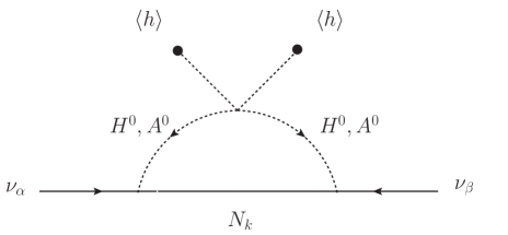
Figure 1: Feynman diagram responsible for the neutrino mass.

Note that the $Z_{2}$ symmetry forbids the term $Y_{ij}\bar{L}_{i}HN_{j}$ in the Lagrangian, and hence rendering neutrinos massless at the tree level. However they get mass at the one loop level (see Fig. 1), given

$$m_{\alpha\beta}^{(\nu)}=\sum_{k}\frac{h_{\alpha k}h_{\beta k}M_{k}}{32\pi^{2}}\left[\frac{m_{H^{0}}^{2}}{m_{H^{0}}^{2}-M_{k}^{2}}\ln\frac{m_{H^{0}}^{2}}{M_{k}^{2}}-\frac{m_{A^{0}}^{2}}{m_{A^{0}}^{2}-M_{k}^{2}}\ln\frac{m_{A^{0}}^{2}}{M_{k}^{2}}\right].$$ (11)

If the mass splitting $m_{H^{0}}^{2}-m_{A^{0}}^{2}=\frac{1}{2}|\lambda_{5}|\upsilon^{2}$ is small with respect to the average $\bar{m}^{2}=(m_{H^{0}}^{2}+m_{A^{0}}^{2})/2$, which is favored by the Electroweak precision measurements, then the expression of the mass matrix elements is simplified to

$$m_{\alpha\beta}^{(\nu)}\simeq\frac{|\lambda_{5}|\upsilon^{2}}{16\pi^{2}}\sum_{k}\frac{h_{\alpha k}h_{\beta k}M_{k}}{\bar{m}^{2}-M_{k}^{2}}\left[1-\frac{M_{k}^{2}}{\bar{m}^{2}-M_{k}^{2}}\ln\frac{\bar{m}^{2}}{M_{k}^{2}}\right].$$ (12)

The neutrino mass matrix elements in (12) can be related to the elements of the Pontecorvo-Maki-Nakawaga-Sakata (PMNS) mixing matrix Pontecorvo:1967fh elements. We parametrize the latter as

$$U_{\nu}=\left(\begin{array}[]{ccc}c_{12}c_{13}&c_{13}s_{12}&s_{13}e^{-i\delta_{d}}\\ -c_{23}s_{12}-c_{12}s_{13}s_{23}e^{i\delta_{d}}&c_{12}c_{23}-s_{12}s_{13}s_{23}e^{i\delta_{d}}&c_{13}s_{23}\\ s_{12}s_{23}-c_{12}c_{23}s_{13}e^{i\delta_{d}}&-c_{12}s_{23}-c_{23}s_{12}s_{13}e^{i\delta_{d}}&c_{13}c_{23}\end{array}\right)\times U_{m},$$ (13)

with $\delta_{d}$ the Dirac phase and $U_{m}=\mathrm{diag}(1,\,e^{i\theta_{\alpha}/2},\,e^{i\theta_{\beta}/2})$ encoding the Majorana phase dependence. The shorthand $s_{ij}\equiv\sin\theta_{ij}$ and $c_{ij}\equiv\cos\theta_{ij}$ refers to the mixing angles. For our numerical scans (discussed below) we fit to the best-fit experimental values for the mixing angles and mass-squared differences: $s_{12}^{2}=0.320_{-0.017}^{+0.016}$, $s_{23}^{2}=0.43_{-0.03}^{+0.03}$, $s_{13}^{2}=0.025_{-0.003}^{+0.003}$, $|\Delta m_{13}^{2}|=2.55_{-0.09}^{+0.06}\times 10^{-3}\mathrm{eV}^{2}$ and $\Delta m_{21}^{2}=7.62_{-0.19}^{+0.19}\times 10^{-5}\mathrm{eV}^{2}$ Tortola:2012te . Furthermore, we require that the contribution to neutrino-less double beta decay in this model satisfies the current bound. Within these ranges, one determines the parameter space where viable neutrino masses and mixing occur in the model.

II.2 Theoretical and Experimental Constraints

Here, we discuss different theoretical and experimental constraints on the model parameters.

Theoretical Constraints:

The parameters of the scalar potential have to satisfy these theoretical constraints:

• Perturbativity: all the quartic couplings of the physical fields should be less than $4\pi$, i.e.,

  $$\lambda_{1},\lambda_{2},\left|\lambda_{3}+\frac{1}{2}\lambda_{4}\right|,\left|\lambda_{3}+\frac{1}{2}(\lambda_{4}\mp\lambda_{5})\right|\leq 4\pi.$$ (14)

• Vacuum Stability: the scalar potential is required to be bounded from below in all the directions of the field space. In both field planes $h$–$H^{0}$ and $G^{0}$–$A^{0}$ the following the condition must be satisfied Klimenko

  $$\lambda_{1},\lambda_{2},\lambda_{3}+\frac{1}{2}(\lambda_{4}+\lambda_{5})+\sqrt{\lambda_{1}\lambda_{2}}>0,$$ (15)

  whereas in the plane $H^{{}^{\pm}}$–$G^{{}^{\mp}}$, we find

  $$\lambda_{3}+\frac{1}{2}\lambda_{4}+\frac{2}{3}\sqrt{\lambda_{1}\lambda_{2}}>0.$$ (16)

  In addition, we should consider the condition

  $$\frac{\mu_{1}^{2}}{\sqrt{\lambda_{1}}}\geq-\frac{\mu_{2}^{2}}{\sqrt{\lambda_{2}}},$$ (17)

  which is required to guarantee that the inert vacuum is the global minimum Ginzburg:2010wa .

• Perturbative unitarity: We demand that the perturbative unitarity is preserved in variety of processes involving scalars or gauge bosons at high energy. At high energies, the equivalence theorem replaces the $W$ and $Z$ bosons by the Goldstone bosons. Computing the decay amplitudes for these processes, one finds a set of $4$ matrices with quartic couplings as their entries Akeroyd:2000wc . The diagonalization of the scattering matrix gives the following eigenvalues

  $$e_{1,2} = \lambda_{3}\pm\frac{\lambda_{4}}{2},~{}e_{3,4}=\lambda_{3}\pm\frac{\lambda_{5}}{2},~{}e_{5,6}=\lambda_{3}+\lambda_{4}\pm\frac{3}{2}\lambda_{5},~{}e_{7,8}=-\frac{\lambda_{1}+\lambda_{2}}{6}\pm\sqrt{\left(\frac{\lambda_{1}+\lambda_{2}}{6}\right)^{2}+\frac{\lambda_{4}^{2}}{4}},$$

  $$e_{9,10} = -\frac{\lambda_{1}+\lambda_{2}}{2}\pm\sqrt{9\left(\frac{\lambda_{1}-\lambda_{2}}{6}\right)^{2}+\left(2\lambda_{3}+\frac{\lambda_{4}}{2}\right)^{2}},~{}e_{11,12}=-\frac{\lambda_{1}+\lambda_{2}}{6}\pm\sqrt{\left(\frac{\lambda_{1}-\lambda_{2}}{6}\right)^{2}+\frac{\lambda_{5}^{2}}{4}}.$$ (18)

  We require that the largest eigenvalue of these matrices to be smaller than $4\pi$.

Experimental Constraints

• Gauge bosons decay widths: in order to keep the $W$ and $Z$ gauge bosons decay modes unmodified, one needs to impose the following conditions:

  $$m_{H^{0}}+m_{A^{0}}>M_{Z}~{},~{}m_{H^{\pm}}+m_{A^{0}}>M_{W},$$

  $$2m_{H^{\pm}}>M_{Z}~{},~{}m_{H^{\pm}}+m_{H^{0}}>M_{W}.$$ (19)

• Lepton flavor violation (LFV) processes: in this model, LFV decay processes arise at one-loop level with the exchange of $H^{\pm}$ and $N_{k}$ particles. The branching ratio of the decay $\ell_{\alpha}\rightarrow\ell_{\beta}+\gamma$ due to the contribution of the interactions (2) is Toma:2013zsa .

  $$Br(\ell_{\alpha}\rightarrow\ell_{\beta}+\gamma)=\frac{3\alpha\upsilon^{4}}{32\pi m_{H^{\pm}}^{4}}\left|\sum_{i=1}^{3}h_{\beta i}^{\ast}h_{\alpha i}F\left(M_{i}^{2}/m_{H^{\pm}}^{2}\right)\right|^{2},$$ (20)

  where $\alpha=e^{2}/4\pi$ is the electromagnetic fine structure constant and $F\left(x\right)=\left(1-6x+3x^{2}+2x^{3}-6x^{2}\log x\right)/6\left(1-x\right)^{4}$. We will consider also the LFV decays $\ell_{\alpha}\rightarrow\ell_{\beta}\ell_{\beta}\ell_{\beta}$, where their branching ratio formulas are given in Toma:2013zsa . In our numerical scan, we will impose all the experimental limits on both $Br(\ell_{\alpha}\rightarrow\ell_{\beta}+\gamma)$ and $Br(\ell_{\alpha}\rightarrow\ell_{\beta}\ell_{\beta}\ell_{\beta})$  Patrignani:2016xqp .

• The electroweak precision tests: while taking $\Delta U=0$ in our analysis, the oblique parameters can be written in our model as Grimus:2008nb

  $$\varDelta T = \frac{1}{16\pi s_{\mathrm{w}}^{2}M_{W}^{2}}\left\{F\left(m_{H^{0}}^{2},m_{H^{\pm}}^{2}\right)+F\left(m_{A^{0}}^{2},m_{H^{\pm}}^{2}\right)-F\left(m_{H^{0}}^{2},m_{A^{0}}^{2}\right)\right\},$$

  $$\varDelta S = \frac{1}{24\pi}\left\{\left(2s_{\mathrm{w}}^{2}-1\right)^{2}G\left(m_{H^{\pm}}^{2},m_{H^{\pm}}^{2},M_{Z}^{2}\right)+G\left(m_{H^{0}}^{2},m_{A^{0}}^{2},M_{Z}^{2}\right)+\ln\left(\tfrac{m_{H^{0}}^{2}m_{A^{0}}^{2}}{m_{H^{\pm}}^{4}}\right)\right\},\hskip 14.22636pt$$ (21)

  where $s_{\mathrm{W}}\equiv\sin~{}\theta_{W}$, with $\theta_{W}$ is the Weinberg mixing angle, and the functions $F$ and $G$ are loop integrals that are given in the literature Grimus:2008nb .

• The ratio $R_{\gamma\gamma}$: The existence of the charged scalar $H^{\pm}$ modifies the value of the branching ratio $\mathcal{B}(h\rightarrow\gamma\gamma)$, which both ATLAS and CMS collaborations have reported their combined results on the ratio $R_{\gamma\gamma}:=\mathcal{B}(h\to\gamma\gamma)/\mathcal{B}(h\to\gamma\gamma)^{SM}=1.09\pm 0.12$ ATLAS:2017ovn . In the model we are considering, $R_{\gamma\gamma}$ reads

  $$R_{\gamma\gamma}=\left|1+\frac{\lambda_{3}\upsilon^{2}}{2m_{H^{\pm}}^{2}}\frac{A_{0}^{\gamma\gamma}\left(\frac{m_{h}^{2}}{4m_{H^{\pm}}^{2}}\right)}{A_{1}^{\gamma\gamma}\left(\frac{m_{h}^{2}}{4M_{W}^{2}}\right)+N_{c}Q_{t}^{2}A_{1/2}^{\gamma\gamma}\left(\frac{m_{h}^{2}}{4m_{t}^{2}}\right)}\right|^{2},$$ (22)

  where the functions $A_{i}^{\gamma\gamma}$ are given in Chen:2013vi . Another Higgs decay branching ratio that gets modified is $h\rightarrow\gamma Z$, with the signal strength is given by

  $$R_{\gamma Z}=\left|1-\frac{1-2s_{\mathrm{w}}^{2}}{c_{\mathrm{w}}}\frac{\lambda_{3}\upsilon^{2}}{2m_{H^{\pm}}^{2}}\frac{A_{0}^{\gamma Z}\left(\frac{m_{h}^{2}}{4m_{H^{\pm}}^{2}},\frac{M_{Z}^{2}}{4m_{H^{\pm}}^{2}}\right)}{c_{\mathrm{w}}A_{1}^{\gamma Z}\left(\frac{m_{h}^{2}}{4M_{W}^{2}},\frac{M_{Z}^{2}}{4M_{W}^{2}}\right)+\frac{6-16s_{\mathrm{w}}^{2}}{3c_{\mathrm{w}}}A_{1/2}^{\gamma Z}\left(\frac{m_{h}^{2}}{4m_{t}^{2}},\frac{M_{Z}^{2}}{4m_{t}^{2}}\right)}\right|^{2},$$ (23)

  where $c_{\mathrm{w}}^{2}=1-s_{\mathrm{w}}^{2}$ and the functions $A_{i}^{\gamma Z}$ are given in Chen:2013vi . The branching ratio $h\rightarrow\gamma Z$ is not measured yet, but when it will be measured with a good precision, it can give a hint about the extra charged scalar whether it is a singlet or it belongs to a higher order multiplet.

• LEP direct searches of charginos and neutralinos: The search for the inert particles have never been done at colliders. However, their signature is very similar to those of neutralinos and charginos in supersymmetric models Abdallah:2003xe . We take a conservative approach and impose the following lower bounds

  $$m_{H^{\pm}}>113.5~{}\text{GeV}~{},\quad\max\{m_{H^{0}},m_{A^{0}}\}>100~{}\text{GeV},$$ (24)

  where the last bound comes from a re-interpretation of neutralino searches at LEP Lundstrom:2008ai in the context of the IHDM.

• Dark matter relic density: In this model, we are considering the lightest right handed neutrino to be the DM candidate. Its annihilation occurs onto SM neutrinos and charged leptons via t-channel diagrams mediated by the members of the Inert doublet. After computing the thermally averaged cross section Gondolo:1990dk , $<\sigma_{N_{1}N_{1}}v_{r}>=<\sigma(N_{1}N_{1}\rightarrow\ell^{+}\ell^{-},\nu\bar{\nu})v_{r}>$, the DM relic abundance can be expressed as Jungman:1995df

  $$\Omega_{N_{1}}h^{2}\simeq\frac{3\times 10^{-26}~{}\text{cm}^{3}s^{-1}}{<\sigma_{N_{1}N_{1}}v_{r}>},$$ (25)

  which we require to be in agreement with the measured values by WMAP Hinshaw:2012aka and Planck Ade:2015xua collaborations. The expression of the relic density in (25) is estimated without taking into account the co-annihilation effect. Such effect can be important when $N_{2}$ and/or $N_{3}$ have masses very close to that of $N_{1}$, i.e., $\Delta_{i}=(M_{i}-M_{1})/M_{1}\ll 1$, and hence one should not neglect it when computing the relic density. However, co-annihilation with the inert members, such as the process $N_{1}H^{\pm}\rightarrow\ell_{\alpha}\gamma$, is less important due to the smallness the electromagnetic coupling as compared to the Yukawa couplings $h_{ik}$.

  In order to account for such effect, one substitute $<\sigma_{N_{1}N_{1}}v_{r}>$ in (25) by the thermal average of the effective cross section Kong:2005hn

  $$\sigma_{eff}(x_{f}) = \sum_{i,k}^{3}\tfrac{2^{2}}{g_{eff}^{2}}\left(1+\Delta_{i}\right)^{3/2}\left(1+\Delta_{k}\right)^{3/2}e^{-x_{f}\left(\Delta_{i}+\Delta_{k}\right)}\left\langle\sigma_{ik}v_{r}\right\rangle$$ (26)

  with

  $$g_{eff}(x_{f}) = \sum_{i}^{3}2\left(1+\Delta_{i}\right)^{3/2}e^{-x_{f}\Delta_{i}},$$ (27)

  Here, $x_{f}=M_{1}/T_{f}$ is the freeze-out parameter, $g_{eff}(x_{f})$ accounts for the effective multiplicity at the freeze-out, and $\left\langle\sigma_{ik}v_{r}\right\rangle$ is the thermally averaged cross section of $N_{i}N_{k}\rightarrow\ell_{\alpha}^{-}\ell_{\beta}^{+},\nu_{\alpha}\bar{\nu}_{\beta}$ at the freeze-out. Here, the ratio

  $$\Delta_{i}=\frac{M_{i}-M_{1}}{M_{1}},$$ (28)

  is the relative mass difference. The cross section formulas for the processes $N_{i}N_{k}\rightarrow\ell_{\alpha}^{-}\ell_{\beta}^{+},\nu_{\alpha}\bar{\nu}_{\beta}$ are given in Eq. (36) in the appendix.

• Dark matter direct detection: Although $N_{1}$ does not couple directly to the Higgs boson or $Z$ gauge boson, it acquire an effective vertex $hN_{1}\bar{N}_{1}$ at one loop. In this case, the spin independent (SI) scattering cross section of $N_{1}$ off a nucleon ${\cal N}$ reads

  $$\sigma_{det}(N_{1}+{\cal N}\rightarrow N_{1}+{\cal N}) = \frac{\tilde{y}_{hN_{1}\bar{N}_{1}}^{2}(m_{{\cal N}}-\frac{7}{9}m_{{\cal B}})^{2}m_{{\cal N}}^{2}M_{1}^{2}}{4\pi\upsilon^{2}m_{h}^{4}(m_{{\cal N}}+M_{1})^{2}},$$ (29)

  where $m_{{\cal N}}$ and $m_{{\cal B}}$ are the nucleon and baryon masses in the Chiral limit He:2008qm , and $\tilde{y}_{hN_{1}\bar{N}_{1}}$ is the induced one loop effective dark matter coupling to the Higgs boson. There are three generic contributions to the effective $\tilde{y}_{hN_{1}\bar{N}_{1}}$ coupling that lead to the SI interaction as are shown in Fig. 2.

  

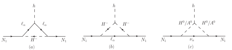
  Figure 2: Feynman diagrams that are responsible to the effective coupling $\tilde{y}_{hN_{1}\bar{N}_{1}}$.

  In non-relativistic limit and $m_{\ell_{\alpha}}\ll M_{1}$, the effective coupling can be approximated by Okada:2013rha

  $$\tilde{y}_{hN_{1}N_{1}} = -\frac{\lambda_{3}\upsilon\sum_{\alpha}|h_{\alpha 1}|^{2}}{16\pi^{2}M_{1}^{3}}\left(M_{1}^{2}+\left(m_{H^{\pm}}^{2}-M_{1}^{2}\right)ln\left(\frac{m_{H^{\pm}}^{2}-M_{1}^{2}}{m_{H^{\pm}}^{2}}\right)\right)$$ (30)

  $$-\frac{\left(\lambda_{3}+\lambda_{4}/2\right)\upsilon\sum_{\alpha}|h_{\alpha 1}|^{2}}{16\pi^{2}M_{1}^{3}}\left(M_{1}^{2}+\left(\bar{m}^{2}-M_{1}^{2}\right)ln\left(\frac{\bar{m}^{2}-M_{1}^{2}}{\bar{m}^{2}}\right)\right),$$

  where $\bar{m}^{2}=(m_{H^{0}}^{2}+m_{A^{0}}^{2})/2$. In the above expression, the first [second] line corresponds to diagram (b), and the second line [(c)], whereas diagram (a) contribution is negligible since it is $m_{\ell_{\alpha}}^{2}/m_{H^{\pm}}^{2}$ proportional. Thus, in our scan of the parameter space we will impose the recent bounds on the dark matter-nucleon scattering cross section from the LUX Akerib:2016vxi and XENON1T Aprile:2017iyp direct detection experiments.

III Numerical Analysis and Discussion

The model contains 26 free parameters: 4 quartic couplings in the scalar potential $\lambda_{i},i=2..5$, 18 (9 complex) Yukawa couplings $h_{ij},i,j=1..3$, 3 RHNs masses $M_{k},k=1..3$ and the squared-mass parameter $\mu_{2}^{2}$ of the inert Higgs. In our numerical analysis, we perform a scan of those parameters over the parameters ranges

$$0<\lambda_{2},|\lambda_{3,4}|<2,$$

$$1\textrm{ GeV}<M_{1}<M_{2}<M_{3}<2\textrm{ TeV},$$

$$-\upsilon^{2}<\mu_{2}^{2}<7\upsilon^{2},\qquad 10^{-5}<|h_{ij}|<1.$$ (31)

Taking into account all theoretical and experimental constraints mentioned in the previous section, we scan over the parameters range (31). Within this parameters range, one can estimate the effect of the one-loop corrections in (9) on the observables $X=\lambda,\,\mu^{2}$, by showing the ratio $\delta X=\left(X-X_{tree-level}\right)/X_{tree-level}$ in Fig. 3, where we consider 3000 benchmark points that fulfill all the conditions mentioned in the previous section.

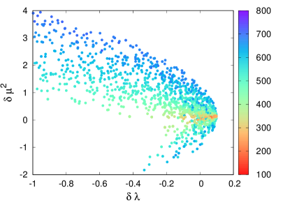
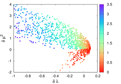
Figure 3: The ratios $\delta\lambda$ and $\delta\mu^{2}$ that represent the relative corrections due to the inert members. In the palette, we read the large inert members mass (right) and its coupling to the Higgs, i.e., $|\lambda_{3}|$ ($|\lambda_{3}+\lambda_{4}/2\pm\lambda_{5}/2|$) if $m_{H^{+}}>m_{H^{0},A^{0}}$ ($m_{H^{+}}<m_{H^{0},A^{0}}$).

One has to notice that the one-loop effect is very important for massive and strongly coupled inert members. For instance, the inert corrections in (9) gives $\delta\lambda=-1\sim 0.098$ and $\delta\mu^{2}=-1.83\sim 3.94$, i.e., the Higgs mass and quartic coupling could be fully radiative $\delta\lambda\sim-1$.

In Fig. 4, we depict the DM relic density, co-annihilation effect and the direct detection spin-independent cross section as a function of the DM mass for the benchmark points used in Fig. 3.

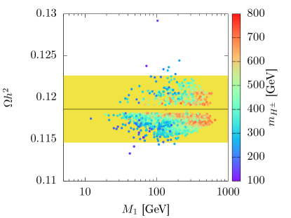
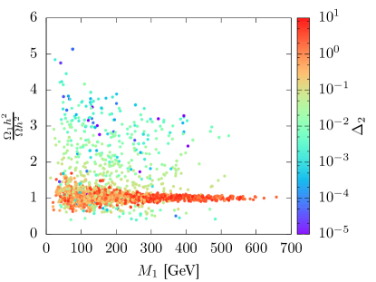
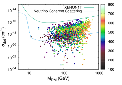
Figure 4: Top left: the relic density of the DM as a function of its mass. The yellow band shows the experimental measurement of $\Omega_{N_{1}}h^{2}$ at $2\sigma$. Top right: the ratio of $\Omega_{1}h^{2}/\Omega h^{2}$, where $\Omega_{1}h^{2}$ ($\Omega h^{2}$) does (not) include the co-annihilation effect. The palette represents the degeneracy parameter $\Delta_{2}$ defined in (28). Bottom: the direct detection cross section as a function of the DM mass, with the exclusion plot obtained from the Xenon1T experiment. The blue curve represents the irreducible neutrino background due to the coherent neutrino-nucleus scattering.

From Fig. 4, one remarks that: (1) most of the benchmark points are within the $1\sigma$ envelope on the relic density measurement. (2) We see that the lightest RHN can be a viable DM candidate for masses in the range $10-700~{}\textrm{GeV}$ and with a spin-independent direct detection cross section below the experimental bound. Note that a large fraction of the benchmark points are above the irreducible neutrino background and hence can be probed in future direct detection experiments. (3) The ratio co-annihilation effect that is presented with the ratio $\Omega_{1}h^{2}/\Omega h^{2}$, where $\Omega_{1}h^{2}$ ($\Omega h^{2}$) refers to the relic density within (without) the co-annihilation effect. As expected, the co-annihilation effect is important only for benchmark points where the two RHN’s ($N_{1},N_{2}$) are degenerate, i.e., very small mass difference values. It is worth mentioning that even though one could allow $M_{1}$ to vary over the mass range in (31), for DM heavier than $700~{}GeV$ the relic density requires the couplings $h_{i,1}$ to be much larger than unity so that the relic density will be in agreement with the observed value. However, this will make the constraints on the LFV processes very difficult to satisfy.

For the same benchmark points, we present in Fig. 5, the different branching fractions of the LFV processes $\ell_{\alpha}\to\ell_{\beta}+\gamma$ (left panel) and $\ell_{\alpha}\to 3\ell_{\beta}$ (right panel), normalized to their experimental bounds, versus the DM mass. We Note that the stringent lepton flavor violation constraint comes from the process $\mu\to e\gamma$, where it is severely fulfilled for most of the benchmark points. This could be achieved by cancellation between different terms in (20), since the right relic density value does not allow the Yukawa couplings to have smaller values.

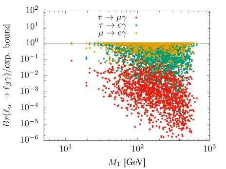
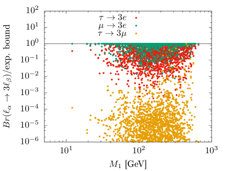
Figure 5: The branching ratios $\text{Br}(\ell_{\alpha}\to\ell_{\beta}+\gamma)$ (left) and $\text{Br}(\ell_{\alpha}\to 3\ell_{\beta})$ (right) normalized by their experimental bounds as a function of $M_{1}$

In Fig. 6-left, we depict the oblique parameters $S$ versus $T$ where the different ellipses represent the $68\%$, $95\%$ and $99\%$ CL intervals obtained from the precise measurements of various observables. The color map shows a ratio defined by

$$\Delta=\frac{2m_{H^{\pm}}-m_{A^{0}}-m_{H^{0}}}{2m_{H^{\pm}}},$$ (32)

which parametrizes how close is the charged Higgs mass to the arithmetic mean of the CP-even and CP-odd Higgs masses. In the right panel of Fig. 6, we show $R_{\gamma\gamma}$ vs $R_{\gamma Z}$. As can be seen from left panel in the figure, one remarks that the electroweak precision tests exclude the benchmark points with larger values of the parameter $\Delta$. From Fig. 6-right, one can see that the two branching ratios are proportional to each other due to the nature of the new additional scalar multiplet, i.e., the inert doublet. This can be understood from the factor $(1-2s_{\mathrm{w}}^{2})/c_{\mathrm{w}}$ in (23).

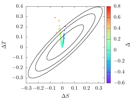
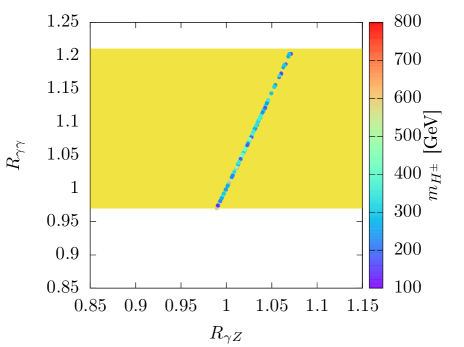
Figure 6: Left: Constraints due to oblique parameters $S$ and $T$ with the palette showing the ratio $\Delta$ defined in (32). Right: the scatter plot of ($R_{\gamma\gamma}$,$R_{\gamma Z}$), where the palette shows the value of $m_{H^{\pm}}$ allowed by theoretical and experimental constraints. The yellow band in the right panel shows the $1\sigma$ interval of $R_{\gamma\gamma}$ of both ATLAS and CMS.

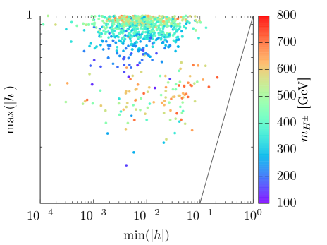
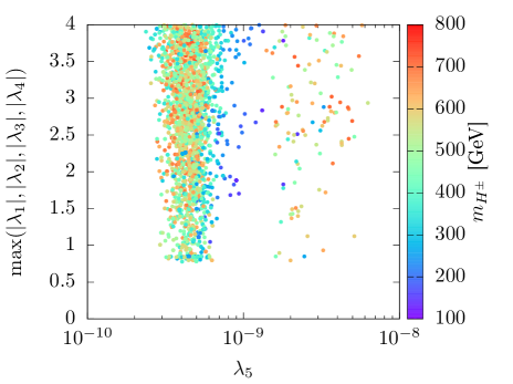
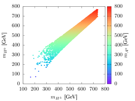
Figure 7: Allowed model parameters by various constraints. Top left: $\max(|h|)$ versus $\min(|h|)$ where $h\equiv h_{ij}$ are the new Yukawa couplings (2). Top right: $\max(\lambda_{1},\lambda_{2},|\lambda_{3}|,|\lambda_{4}|)$ versus $\lambda_{5}$. Bottom panel: scatter plot of $m_{H^{\pm}}$ versus $m_{H^{0}}$, where $m_{A^{0}}$ is shown in the palette.

We give in Fig. 7 the range of parameter space of the model after passing all the theoretical and experimental constraints, leading to the results presented in the previous figures. In the left top panel, we show $\min(|h|)$ versus $\max(|h|)$ where $h\equiv h_{ij}$ are the new Yukawa couplings. The line displayed in that figure define the regime couplings are degenerate couplings regime, and farther from it the less degenerate the couplings are. Moreover, the Yukawa h-couplings values that fit the neutrino oscillation, fulfill the LFV and the relic density have the same order of magnitude whether the CP violating phases are vanishing or not. Thus, in this model there is no favored values or range of CP violating phases. Furthermore, in both cases of normal and inverted neutrino mass hierarchy, the allowed parameter space is similar. For the case of real Yukawa h-couplings, they need to be about one order of magnitude smaller than the complex case of complex, which is due to the fact that the cancellations in (20) required to fulfill the LFV constraints is much easier to achieve for complex valued Yukawa couplings than real ones.

In the right top panel of the same figure, we show $\max(|\lambda_{1,2,3,4}|)$ as a function of the coupling $|\lambda_{5}|$. One can see that $\lambda_{5}$ take very small values, and this is required to be in agreement with the observed neutrino masses and mixing angles. This allow the new Yukawa couplings $h_{ij}$ to be unsuppressed as opposed to the case considered in Ma:2006km . The bottom panel, represents the allowed masses of the CP-odd scalar, $m_{A^{0}}$, projected on the $(m_{H^{0}},m_{H^{\pm}})$ plan. The implication of the smallness of $\lambda_{5}$ is that the CP-odd and CP-even states are quasi degenerate, which render the constraints on the oblique parameters easy to satisfy.

IV Collider phenomenology

IV.1 Possible signatures

The RHNs, $N_{i}$, can be pair produced through several processes both at hadron as well at lepton colliders. At hadron colliders, however, it cannot be produced directly because of the absence of the vertices $Z^{0}N\bar{N}$, $\gamma N\bar{N}$ and $hN\bar{N}$ in this model, and can only be found in the decay products of the inert doublet members. At lepton colliders such as the ILC or the FCC-ee, $N_{i}$ can be produced in $t$-channel processes with charged boson exchange. For the lightest RHN, $N_{1}$, when produced at colliders, it is accounted as missing energy, however, $N_{2}$ and $N_{3}$ depending on their decay width $\Gamma(N_{2,3}\rightarrow N_{1}+\ell^{+}\ell^{-})$ may or may not behave as missing energy. This depends on the decay lengths $l_{i}=E_{i}/M_{i}/\Gamma_{N_{i}}$ (i=2,3), with $E_{i}$ and $\Gamma_{N_{i}}$ are the energy and total decay width of $N_{i}$, respectively.

From the different theoretical and experimental constraints, especially from neutrino mass and the electroweak precision observables, the neutral scalar particles are degenerate and hence the decays such as $A^{0}\to H^{0}Z^{0}$ are kinematically forbidden. Thus, these particles can only undergo invisible decays (if kinematically allowed) into a RHN $N_{i}$ and a SM neutrino. At the LHC, the charged Higgs boson can be produced in pair or in association with $A^{0}/H^{0}$ with $\sigma\simeq 200$ fb for light charged Higgs boson mass in the $H^{0}H^{\pm}(A^{0}H^{\pm})$ mode (see Fig. 8). This channel, for $\Delta_{H^{\pm}}=m_{H^{\pm}}-m_{H^{0},A^{0}}<M_{W^{\pm}}$, leads exclusively to the spectacular mono-lepton signature. While dilepton signals can be observed in the case of the pair production of charged Higgs boson again for $\Delta_{H^{\pm}}<M_{W^{\pm}}$. On the other hand, for $\Delta_{H^{\pm}}>M_{W^{\pm}}$, the decays $H^{\pm}\to A^{0}/H^{0}W^{\pm}$ are kinematically allowed and hence a wide range of signatures are possible (see Table 1). For the case of $H^{0}H^{0}$ ($A^{0}A^{0}$ or $H^{0}A^{0}$) channels, the two particles decay exclusively into a $N_{i}\nu_{\ell}$ giving a mono-jet or mono-photon signature where the additional jet/photon is produced from Initial State Radiation (ISR) off the scattered quarks. However, due to the large $\alpha_{s}(Q)/\alpha_{\textrm{em}}(Q)$ ratio, QCD radiation is dominant and mono-jet signature is more relevant in this case.

At lepton colliders, the $N_{1}$ can be pair produced through $H^{\pm}$ exchange leading to mono-photon signature where the additional photon is emitted either from the $e^{\pm}$ lines or from the intermediate charged Higgs boson. Pair production of charged Higgs boson or a CP-odd (CP-even) particle is also possible at lepton colliders. In table 1, we summarize the different signatures that can be used to either look for $N_{1}$ in the next LHC-run or to constrain the model using the old measurements.

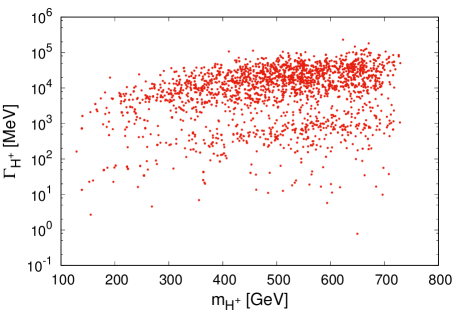
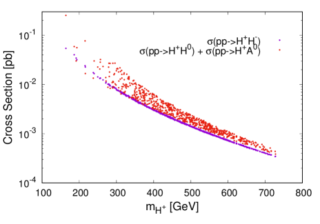
Figure 8: Total width of the charged Higgs boson (left panel) and its inclusive cross section (right panel) as a function of of $m_{H^{\pm}}$.

In Fig. 8, we show the total decay width of the charged Higgs (left) as a function of its mass for some of the benchmarks used previously. We see that the width can be as large as few hundred of GeV for heavy charged Higgs bosons. The reason is that scalar decays $H^{\pm}\to W^{\pm}A^{0}/H^{0}$ are kinematically allowed in certain regions of the parameter space. In the right panel, we present the cross section at the LHC at $\sqrt{s}=14$ TeV of $H^{\pm}H^{\mp}$ and $H^{\pm}H^{0}(A^{0})$ as a function of the charged Higgs mass. We can see that the $H^{\pm}H^{0}(A^{0})$ have larger cross sections and approache $200$ fb for light charged Higgs boson. We stress that for heavy scalar masses, the production cross section is extremely small. This makes the observation of the new states extremely difficult at moderate luminosities.

Process Decay mode signature $pp,e^{+}e^{-}\to H^{\pm}H^{\mp}$ $H^{\pm}\to W^{\pm}H^{0}/A^{0}\to q_{1}\bar{q}_{2}N_{1}\nu_{\ell}$, $H^{\mp}\to W^{\mp}H^{0}/A^{0}\to q_{3}\bar{q}_{4}N_{1}\bar{\nu}_{\ell}$ $4\textrm{ jets}+\not{E}_{T}$ $H^{\pm}\to W^{\pm}H^{0}/A^{0}\to\ell^{\pm}\nu_{\ell}N_{1}\nu_{\ell}$, $H^{\mp}\to W^{\mp}H^{0}/A^{0}\to q_{3}\bar{q}_{4}N_{1}\bar{\nu}_{\ell}$ $1\ell+2\textrm{ jets}+\not{E}_{T}$ $H^{\pm}\to W^{\pm}H^{0}/A^{0}\to\ell_{1}^{\pm}\nu_{\ell}N_{1}\nu_{\ell}$, $H^{\mp}\to W^{\mp}H^{0}/A^{0}\to\ell_{2}^{\mp}\bar{\nu}_{\ell}N_{1}\nu_{\ell}$ $2\ell+\not{E}_{T}$ $H^{\pm}\to W^{\pm}H^{0}/A^{0}\to\ell_{1}^{\pm}\nu_{\ell}N_{1}\nu_{\ell}$, $H^{\mp}\to\ell_{2}^{\mp}N_{1}$ $2\ell+\not{E}_{T}$ $H^{\pm}\to W^{\pm}H^{0}/A^{0}\to q_{1}\bar{q}_{2}N_{1}\nu_{\ell}$, $H^{\mp}\to\ell^{\mp}N_{1}$ $1\ell+2\textrm{ jets}+\not{E}_{T}$ $pp,e^{+}e^{-}\to H^{\pm}H^{0}/A^{0}$ $H^{\pm}\to W^{\pm}H^{0}/A^{0}\to q_{1}\bar{q}_{2}N_{1}\nu_{\ell}$, $H^{0}\to N_{1}\nu_{\ell}$ $1\ell+2\textrm{ jets}+\not{E}_{T}$ $H^{\pm}\to W^{\pm}H^{0}/A^{0}\to\ell^{\pm}\nu_{\ell}N_{1}\nu_{\ell}$, $H^{0}\to N_{1}\nu_{\ell}$ $1\ell+\not{E}_{T}$ $H^{\pm}\to N_{1}\ell^{\pm}$ $1\ell+\not{E}_{T}$ $pp,e^{+}e^{-}\to H^{0}H^{0}$ $H^{0}\to N_{1}\nu_{\ell}$ $\not{E}_{T}+\textrm{ ISR}$ (mono-jet, mono-$\gamma$) $e^{+}e^{-}\to N_{1}N_{1}\gamma$ stable final state $\not{E}_{T}+\gamma$

Table 1: Summary of various signatures of the inert Higgs doublet members and the lightest RHN at the LHC and lepton colliders.

In the rest of this section, we will investigate the monolepton signature at the LHC, that is mentioned in Table. 1.

IV.2 Monolepton signature at the LHC

As a benchmark study, we consider the $1\ell+E_{T}^{\textrm{miss}}$ ($\ell=e,\mu$) final state in $pp$ collisions at $\sqrt{s}=14$ TeV and a luminosity of $300$ fb^-1. Such a signature can arise from $H^{\pm}H^{0}/A^{0}$ production followed by the decay of the charged Higgs either into 1) a charged lepton and a Majorana fermion or 2) a $W$ gauge boson and a dark Higgs where the gauge boson decays leptonically. Feynman diagrams showing the $1\ell+E_{T}^{\textrm{miss}}$ in the signal process are depicted in Fig. 9.

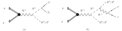
Figure 9: Feynman diagrams for the charged monolepton signature.

Two benchmark points, denoted by BP1 and BP2, are considered in this study where the corresponding parameters are given in Table. 2. Moreover, the chosen benchmarks satisfy all the theoretical and experimental constraints and yield a cross section of order $460$ fb and $127$ fb for BP1 and BP2, respectively. A contribution from $H^{0}H^{0}W^{\pm},A^{0}A^{0}W^{\pm}$ with the $W$-boson decaying leptonically is relevant in BP1 since $\sigma(pp\to H^{0}H^{0}W^{\pm}\to\ell^{\pm}E_{T}^{\mathrm{miss}})\approx 45$ fb. However, the same contribution is very negligible for BP2 and will not be taken into account. Furthermore, they have distinct features regarding collider phenomenology and dark matter relic density. For the first benchmark point (BP1), co-annihilation effects are important since $\Delta_{2}\approx 0.08$, whereas, due to the relatively larger value of $\Delta_{2}$, co-annihilation effects are negligible for the second benchmark (BP2). However, in both scenarios, the decay $H^{\pm}\to W^{\pm}A^{0}/H^{0}\to\ell^{\pm}E_{T}^{\mathrm{miss}}$ has a very small branching ratio, compared to $Br(H^{\pm}\to\ell^{\pm}N_{i})$, which is about $8.27\%$ ($3.21\%$) for BP1 (BP2).

Benchmark Point Parameters $m_{N_{i}}\left(\mathrm{GeV}\right)$ $28.52,~{}30.97,~{}109$, BP1 $m_{H^{\pm}},m_{H^{0}}$ $\left(\mathrm{GeV}\right)$ $164.2,~{}70.49$, $\lambda_{2},\lambda_{3},\lambda_{4},\lambda_{5}$ $2.662,~{}-0.153,~{}-1.451,1.379\times 10^{-10}$, $h_{ij}/10^{-2}$ $\left(\begin{array}[]{ccc}-14.218-i0.997&-2.030-i0.999&62.265-i0.025\\ 69.991+i0.438&-0.544+i0.107&-5.559+i0.719\\ -57.401+i0.980&-0.188+i0.472&-24.365-i0.419\end{array}\right)$, $m_{N_{i}}\left(\mathrm{GeV}\right)$ $17.93,~{}29.27,~{}54.49$, BP2 $m_{H^{\pm}},m_{H^{0}}$ $\left(\mathrm{GeV}\right)$ $215.7,~{}124$, $\lambda_{2},\lambda_{3},\lambda_{4},\lambda_{5}$ $1.069,~{}0.429,~{}-2.05,1.85\times 10^{-10}$, $h_{ij}/10^{-2}$ $\left(\begin{array}[]{ccc}133.45+i5.739&0.239+i0.071&-26.05+i0.57\\ 0.79-i1.028&-2.867+i2.957&78.53-i0.459\\ -68.17+i2.869&0.413+i0.082&-57.06-i1.276\end{array}\right)$.

Table 2: The parameters values the benchmark points BP1 and BP2.

	$\sigma(pp\to H^{\pm}H^{0}/A^{0})$	$Br(W^{\pm}H^{0}/A^{0})$	$\sum_{i}Br(e^{\pm}N_{i})$	$\sum_{i}Br(\mu^{\pm}N_{i})$	$\sum_{i}Br(\tau^{\pm}N_{i})$
BP1	$460.78$ fb	$37.22\%$	$19.74\%$	$24.07\%$	$18.95\%$
BP2	$125.67$ fb	$14.46\%$	$49.62\%$	$16.25\%$	$21.02\%$

Table 3: $H^{\pm}S(S=A^{0},H^{0})$ production cross section and decays branching ratios of the charged Higgs boson in the two benchmark scenarios.

The background contributions to $\ell+E_{T}^{\mathrm{miss}}$ signal can be classified into two categories: irreducible and reducible. The $W$ production followed by its leptonic is the dominant irreducible background with a cross section of order $\mathcal{O}(20)~{}nb$ at Leading Order (LO). Diboson processes, $WZ,WW$ and $ZZ$, contribute as well to the background sources in the $\ell+E_{T}^{\textrm{miss}}$ final state especially $W(\to\ell\nu)Z(\to\nu\bar{\nu})$ which is irreducible. Important contributions might come from $t\bar{t}$ and single top production where the top quark decays leptonically. Furthermore, there are several background processes whose contribution cannot be estimated at the parton level. In such background categories, charged lepton and missing energy arise either from i) multi-jet production where they are produced from hadron decays, and ii) in Drell-Yan process ($Z/\gamma^{*}\to\ell^{+}\ell^{-}$) where one lepton is not detected. We do not consider these background in this study since their contribution can be significantly reduced by imposing isolation cuts and by requiring that the lepton and missing must have a back-to-back topology. These requirements are translated into cuts on the ratio of $p_{T}^{\ell}/E_{T}^{\mathrm{miss}}$ and $\Delta\Phi(\ell,E_{T}^{\mathrm{miss}})$. A perfect balance in the transverse plane between the charged lepton is reached when a charged lepton is produced in association with an invisible particle yielding a ratio $p_{T}^{\ell}/E_{T}^{\mathrm{miss}}\simeq 1$ and an azimuthal separation $\Delta\Phi\simeq\pi$. However, in hadronic collisions, there are QCD radiation off partons in the proton beams which result in a recoil of the lepton and missing energy system and yield a shift in the values $p_{T}^{\ell}/E_{T}^{\mathrm{miss}}$ and $\Delta\Phi(\ell,E_{T}^{\mathrm{miss}})$ but with an unmodified peak position. For reference, in Fig. 10 we show the imbalance between the lepton $p_{T}^{\ell}$ and transverse missing energy in the two benchmark points and the SM background. We can see that for the signal, $W^{\pm}$ and $W^{\pm}Z$, this distribution is peaked around a value about $1$ while it is a smooth function in the case of top quark processes.

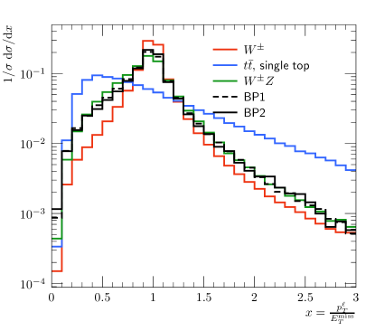
Figure 10: Transverse momentum imbalance between the charged lepton and the missing energy in the two benchmark points and the SM background. The distribution is normalized to unity.

Signal events were generated at LO using CalcHEP Belyaev:2012qa while $W^{\pm}$ and $W^{\pm}Z$ events were generated using Madgraph5_aMC@NLO Alwall:2011uj . PYTHIA8 Sjostrand:2007gs was used for showering and hadronization of the parton level events and for generation of top quark events. Due to its large cross section, $W^{\pm}$ boson events were generated with strong cuts, i.e with $p_{T}^{\ell}>100$ GeV and $E_{T}^{\textrm{miss}}>50$ GeV. Such cuts reduce the total $W$ boson production cross section from $19$ nb to about $6$ pb. While for the other background processes, no cuts were imposed on the generated MC samples. At the analysis level, further cuts are imposed on the charged lepton $p_{T}^{\ell}$ and $E_{T}^{\textrm{miss}}$ to further reduce the SM background contribution. We, first, select events which contains exactly one charged lepton (either electron or muon) with $p_{T}^{\ell}>30$ GeV and $|\eta|<2.4$, and a missing transverse energy (MET) with $E_{T}^{\mathrm{miss}}>30$ GeV. Furthermore, the imbalance between the lepton $p_{T}$ and MET was required to be $0.4<p_{T}^{\ell}/E_{T}^{\mathrm{miss}}<1.4$. Such a cut reduce the amount of events for the signal and the irreducible background by about $20$-$25\%$. However, reducible backgrounds such as $t\bar{t}$ and single top quark production are reduced by a factor of $0.91$. No cuts were imposed on the jet multiplicity, jet $p_{T}$ or $b$-tagging since jet activity is involved in all the processes. We recommend for a more complete analysis to be done at the experimental level. We further refine our selection criteria and define two signal regions; the first signal region is defined by $p_{T}^{\ell}>250$ GeV and $E_{T}^{\mathrm{miss}}>150$ GeV while the second signal region is defined as $p_{T}^{\ell}>250$ GeV and $E_{T}^{\mathrm{miss}}>300$ GeV. In Fig. 11, we show the corresponding distributions for the signal as well as background events.

To quantify the potential discovery of the model in the two benchmark points, we use the general formula for the signal significance which is defined by

$$\mathcal{S}=\sqrt{2\times\left[(N_{\textrm{S}}+N_{\textrm{BG}})\times\log\left(1+\frac{N_{\textrm{S}}}{N_{\textrm{BG}}}\right)-N_{\textrm{S}}\right]},$$ (33)

We compute $\mathcal{S}$ for different values of the cut on the transverse mass of the lepton and missing transverse energy system defined by

$$M_{T}=\sqrt{2p_{T}^{\ell}E_{T}^{\textrm{miss}}(1-\cos\Delta\Phi(\ell,E_{T}^{\textrm{miss}}))}$$ (34)

In Fig. 12, we plot the significance as function of the cut on $M_{T}$ for the two considered benchmark points and in the two signal regions. For $M_{T}^{\mathrm{min}}<1$ TeV, the significance reaches about $5\sigma$ level, and decreases quickly for $M_{T}^{\mathrm{min}}>1$ TeV. This behavior at $M_{T}^{\mathrm{min}}>1$ TeV is due to the relatively low statistics at that region which is a consequence of the light scalars chosen in our benchmark points. On the other hand, benchmark points with heavier scalars hardly achieve the $5\sigma$ level due to the smallness of the corresponding cross section. We notice that in the observability region, systematic uncertainties are quite moderate. They are dominated by uncertainties due to electron and muon energy resolution. Statistical uncertainties are also not important in this region of interest. We found that even for lower luminosities of about $100$ fb^-1, the significance can reach the $5\sigma$ level for $M_{T}^{\mathrm{min}}<600$ GeV in BP1. We leave a more detailed study of all the systematic uncertainties in mono-lepton signatures and interplay with the other channels for a future work  Ahriche:2018 .

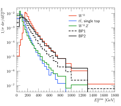
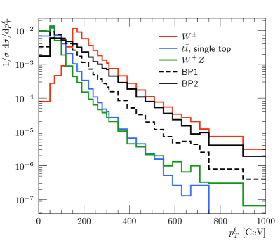
Figure 11: Normalized distributions for missing transverse energy (left panel) and lepton $p_{T}$ (right panel) for signal and background events.

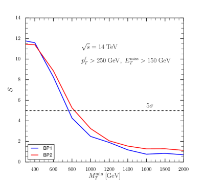
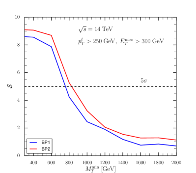
Figure 12: Signal significance as function of $M_{T}^{\mathrm{min}}$ for the first (left panel) and second (right panel) signal regions.

V Conclusion

In this paper, we considered the inert Higgs Doublet Model extended by three right handed neutrinos where both neutrino mass and dark matter are addressed. We considered the DM to be the lightest right handed neutrino and showed that its relic density can be in agreement with the observation provided that Yukawa couplings in the neutrino sector are not highly suppressed. We carried out a detailed numerical analysis to determine the different regions of the parameter space that are consistent with theoretical and experimental constraints. Fitting the observed neutrino mass squared differences and mixing angles requires that the CP-odd and the CP-even components of the inert doublet to have quasi-degenerate masses. We also discussed a number of experimental signatures of this model at high energy colliders. In particular, mono-lepton, mono-jet and mono-photon signals are particularly interesting and can be used to search for the right handed neutrinos both at the LHC and future lepton colliders, such as the ILC. We have performed at detailed analysis of the mono-lepton signature at the LHC and showed that with a $300~{}fb^{-1}$ luminosity it is possible to probe the right handed neutrino signal.

Appendix A The cross section of $N_{i}-N_{k}$ Co-annihilation

In this appendix, we derive the analytic expression annihilation cross of two right handed neutrinos, $N_{i}$ and $N_{k}$, into charged leptons or light neutrinos. For the charged leptons channel, there are two diagrams that contribute to this process, as shown in Fig. 13.

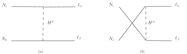
Figure 13: Diagrams contributing to the annihilation $N_{i}N_{k}\rightarrow\ell_{\alpha}^{-}\ell_{\beta}^{+}$. Clearly, the second diagram is possible only if the two RHN’s are identical $(i=k)$. Similar diagrams exit for the channels $N_{i}N_{k}\rightarrow\nu_{\alpha}\bar{\nu}_{\beta}$, where the mediators are $H^{0}/A^{0}$.

After averaging and summing over the initial and final spin states, the corresponding squared amplitude is given by

$$\left|\mathcal{M}\right|^{2} =\frac{\left|g_{i\alpha}g_{k\beta}^{\ast}\right|^{2}}{4}\left[\tfrac{\left(M_{i}^{2}+m_{\ell_{\alpha}}^{2}-t\right)\left(M_{k}^{2}+m_{\ell_{\beta}}^{2}-t\right)}{\left(t-m_{H^{+}}^{2}\right)^{2}}+\delta_{ik}\tfrac{\left(M_{i}^{2}+m_{\ell_{\alpha}}^{2}-u\right)\left(M_{i}^{2}+m_{\ell_{\beta}}^{2}-u\right)}{\left(u-m_{H^{+}}^{2}\right)^{2}}-\delta_{ik}\tfrac{2M_{i}^{2}\left(s-m_{\ell_{\alpha}}^{2}-m_{\ell_{\beta}}^{2}\right)}{\left(t-m_{H^{+}}^{2}\right)\left(u-m_{H^{+}}^{2}\right)}\right],$$ (35)

with $s,t,u$ and $s$ are the Lorentz invariant Mandelstam variables.

After integrating over the phase space, the cross section times the relative velocity of $N_{i}$ and $N_{k}$ reads

$$\upsilon_{r}\sigma =\frac{\left|g_{i\alpha}g_{k\beta}^{\ast}\right|^{2}}{32\pi}\frac{\sqrt{s^{2}-2s\left(m_{\ell_{\alpha}}^{2}+m_{\ell_{\beta}}^{2}\right)+\left(m_{\ell_{\alpha}}^{2}-m_{\ell_{\beta}}^{2}\right)^{2}}}{s^{2}-\left(M_{i}^{2}-M_{k}^{2}\right)^{2}}\left[\tfrac{A_{1}^{2}-B^{2}+Q_{1}Q_{2}}{A_{1}^{2}-B^{2}}-\frac{Q_{1}+Q_{2}}{2B}\log\left|\frac{A_{1}+B}{A_{1}-B}\right|\right|+\delta_{ik}\times$$

$$\left.\left\{\tfrac{A_{2}^{2}-B^{2}+Q_{1}Q_{2}}{A_{2}^{2}-B^{2}}-\frac{Q_{1}+Q_{2}}{2B}log\left|\frac{A_{2}+B}{A_{2}-B}\right|-\frac{M_{i}^{2}\left(s-m_{\ell_{\alpha}}^{2}-m_{\ell_{\beta}}^{2}\right)}{B\left(Q_{1}+Q_{2}-s\right)}\left(\log\left|\frac{A_{1}+B}{A_{1}-B}\right|+\log\left|\frac{A_{2}+B}{A_{2}-B}\right|\right)\right\}\right],$$ (36)

where

$$Q_{1} =M_{i}^{2}+m_{\ell_{\alpha}}^{2}-m_{H^{+}}^{2},~{}Q_{2}=M_{k}^{2}+m_{\ell_{\beta}}^{2}-m_{H^{+}}^{2},$$

$$A_{1} =\frac{M_{i}^{2}+M_{k}^{2}+m_{\ell_{\alpha}}^{2}+m_{\ell_{\beta}}^{2}-2m_{H^{+}}^{2}-s}{2}-\frac{\left(M_{i}^{2}-M_{k}^{2}\right)\left(m_{\ell_{\alpha}}^{2}-m_{\ell_{\beta}}^{2}\right)}{2s},$$

$$A_{2} =M_{i}^{2}-m_{H^{+}}^{2}+\frac{m_{\ell_{\alpha}}^{2}+m_{\ell_{\beta}}^{2}-s}{2},\,B=2\frac{\sqrt{s^{2}-2s\left(m_{\ell_{\alpha}}^{2}+m_{\ell_{\beta}}^{2}\right)+\left(m_{\ell_{\alpha}}^{2}-m_{\ell_{\beta}}^{2}\right)^{2}}}{2\sqrt{s}}p.$$

Here $p=\sqrt{s^{2}-2s\left(M_{i}^{2}+M_{k}^{2}\right)+\left(M_{i}^{2}-M_{k}^{2}\right)^{2}}/2\sqrt{s}$ is the magnitude of the momentum of the incoming RHN in the center of mass frame. The cross section of $\sigma(N_{i}N_{k}\rightarrow\nu_{\alpha}\nu_{\beta}$ can be obtained by simply making the replacement $~{}m_{H^{+}}^{2}\rightarrow\bar{m}^{2}=\frac{1}{2}(m_{H^{0}}^{2}+m_{A^{0}}^{2})$ and $m_{\ell_{\alpha}}^{2}=m_{\ell_{\beta}}^{2}=0,$ in the above expression (36).

In the non-relativistic limit, we can expand the logarithms in (36) in power of $p$, equivalently $B$, to obtain

$$\upsilon_{r}\sigma \approx\frac{\left|g_{i\alpha}g_{k\beta}^{\ast}\right|^{2}}{32\pi}\frac{\sqrt{s^{2}-2s\left(m_{\ell_{\alpha}}^{2}+m_{\ell_{\beta}}^{2}\right)+\left(m_{\ell_{\alpha}}^{2}-m_{\ell_{\beta}}^{2}\right)^{2}}}{s^{2}-\left(M_{i}^{2}-M_{k}^{2}\right)^{2}}\left[\frac{A_{1}-Q-Q_{2}}{A_{1}}+\tfrac{Q_{1}Q_{2}}{A_{1}^{2}}\left(1+\frac{B^{2}}{A_{1}^{2}}\right)\right.$$

$$\left.+\delta_{ik}\left\{\frac{A_{2}-Q_{1}-Q_{2}}{A_{2}}+\tfrac{Q_{1}Q_{2}}{A_{2}^{2}}\left(1+\frac{B^{2}}{A_{2}^{2}}\right)-\frac{2M_{i}^{2}\left(s-m_{\ell_{\alpha}}^{2}-m_{\ell_{\beta}}^{2}\right)}{A_{2}^{2}}\right\}\right].$$

For $i=k=1$, the expression of the annihilation cross section agrees with the one given in Cheung:2004xm .

Appendix B The effective $hN_{1}\bar{N}_{1}$ coupling

Here, we present the different contributions to the effective $hN_{1}\bar{N}_{1}$ coupling in terms of the Passarino-Veltman three-point functions (denoted by $C_{i}$ in what follows). To compute the effective $\tilde{y}_{hN_{1}\bar{N}_{1}}$ coupling, we consider the process $h(p)\to N_{1}(k_{1})+\bar{N}_{1}(k_{2})$, at one-loop level. The corresponding Feynman diagrams are depicted in Fig. 2. The evaluation of the Feynman amplitudes was performed analytically and compared to the result of FeynArts and FormCalc FA2 while numerical evaluations of the coupling were performed with the help of the LoopTools package FF and compared to the approximate result shown in (30). The amplitude of the first contribution (diagram (a) in Fig. 2) can be written as

$$i\Gamma_{a}\left(p,k_{1},k_{2}\right) = \int\frac{d^{4}Q}{\left(2\pi\right)^{4}}\left(-ih_{\alpha 1}^{*}P_{L}\right)\frac{i}{\not{Q}-m_{\ell_{\alpha}}}\left(i\frac{m_{\ell_{\alpha}}}{\upsilon}\right)\frac{i}{\not{Q}+\not{p}-m_{\ell_{\alpha}}}\left(ih_{\alpha 1}P_{R}\right)\frac{i}{\left(k_{1}-Q\right)^{2}-m_{H^{+}}^{2}}$$

$$= h_{\alpha 1}^{*}h_{\alpha 1}\frac{m_{\ell_{\alpha}}}{\upsilon}\int\frac{d^{4}Q}{\left(2\pi\right)^{4}}\frac{P_{L}\left(\not{Q}+m_{\ell_{\alpha}}\right)\left(\not{Q}+\not{p}+m_{\ell_{\alpha}}\right)P_{R}}{\left[Q^{2}-m_{\ell_{\alpha}}^{2}\right]\left[\left(Q-p\right)^{2}-m_{\ell_{\alpha}}^{2}\right]\left[\left(k_{1}-Q\right)^{2}-m_{H^{+}}^{2}\right]}$$

$$= \frac{h_{\alpha 1}^{*}h_{\alpha 1}m_{\ell_{\alpha}}^{2}}{\upsilon}P_{L}\int\frac{d^{4}Q}{\left(2\pi\right)^{4}}\frac{2\not{Q}+\not{p}}{\left[Q^{2}-m_{\ell_{\alpha}}^{2}\right]\left[\left(Q-p\right)^{2}-m_{\ell_{\alpha}}^{2}\right]\left[\left(k_{1}-Q\right)^{2}-m_{H^{+}}^{2}\right]}.$$ (38)

Using the Passarino-Veltman reduction Passarino:1978jh , we find for the first contribution

$$\Gamma_{a}\left(p,k_{1},k_{2}\right) =\frac{1}{16\pi^{2}\upsilon}\sum_{\alpha}|h_{\alpha 1}|^{2}m_{\ell_{\alpha}}^{2}\left\{C_{0}(M_{1}^{2},p^{2},M_{1}^{2},m_{H^{\pm}}^{2},m_{\ell_{\alpha}}^{2},m_{\ell_{\alpha}}^{2})\right.$$

$$+\left.C_{1}(M_{1}^{2},p^{2},M_{1}^{2},m_{H^{\pm}}^{2},m_{\ell_{\alpha}}^{2},m_{\ell_{\alpha}}^{2})+C_{2}(M_{1}^{2},p^{2},M_{1}^{2},m_{H^{\pm}}^{2},m_{\ell_{\alpha}}^{2},m_{\ell_{\alpha}}^{2})\right\}.$$ (39)

The amplitude for the second contribution (diagram (b) in Fig. 2) is given by

$$i\Gamma_{b}\left(p,k_{1},k_{2}\right) =\int\frac{d^{4}Q}{\left(2\pi\right)^{4}}\left(-ih_{\alpha 1}^{*}P_{L}\right)\frac{i}{\not{k}_{1}-\not{Q}-m_{\ell_{\alpha}}}\left(ih_{\alpha 1}P_{R}\right)\frac{i}{\left(p+Q\right)^{2}-m_{H^{+}}^{2}}\left(i\lambda_{3}\upsilon\right)\frac{i}{Q^{2}-m_{H^{+}}^{2}}$$

$$+(P_{L}\longleftrightarrow P_{R}).$$ (40)

After some algebra, we get

$$\Gamma_{b}\left(p,k_{1},k_{2}\right) =-\frac{1}{16\pi^{2}}\lambda_{3}\upsilon M_{1}\sum_{\alpha}|h_{\alpha 1}|^{2}\left\{C_{0}(p^{2},M_{1}^{2},M_{1}^{2},m_{H^{\pm}}^{2},m_{H^{\pm}}^{2},m_{\ell_{\alpha}}^{2})\right.$$

$$+\left.C_{2}(p^{2},M_{1}^{2},M_{1}^{2},m_{H^{\pm}}^{2},m_{H^{\pm}}^{2},m_{\ell_{\alpha}}^{2})\right\}.$$ (41)

The contribution of diagram (c) can be evaluated similarly to give

$$\Gamma_{c}\left(p,k_{1},k_{2}\right) =-\frac{1}{16\pi^{2}}(\lambda_{3}+\lambda_{4}/2)M_{1}\upsilon\sum_{S=H^{0},A^{0}}\sum_{\alpha}|h_{\alpha 1}|^{2}\left\{C_{1}(p^{2},M_{1}^{2},M_{1}^{2},0,m_{S}^{2},m_{S}^{2})\right.$$

$$+\left.C_{2}(p^{2},M_{1}^{2},M_{1}^{2},0,m_{S}^{2},m_{S}^{2})\right\}.$$ (42)

Numerically, we found that the contribution of diagram (a) is much smaller than the contribution of diagrams (b) and (c). Furthermore, in our numerical analysis, we use the expression quoted in (30) since it agrees very well with the full expression in terms of the Passarino-Veltman functions.

- (1) G. Aad et al. [ATLAS Collaboration ], Phys. Lett. B 716, 1 (2012) [arXiv:1207.7214 [hep-ex]]. S. Chatrchyan et al. [CMS Collaboration], Phys. Lett. B 716, 30 (2012) [arXiv:1207.7235 [hep-ex]].
- (2) A. Zee, Phys. Lett. 161B, 141 (1985). E. Ma, Phys. Rev. Lett. 81, 1171 (1998) [hep-ph/9805219].
- (3) A. Zee, Nucl. Phys. B 264, 99 (1986); K. S. Babu, Phys. Lett. B 203, 132 (1988); M. Aoki, S. Kanemura, T. Shindou, and K. Yagyu, J. High Energy Phys. 10 1007 (2010) 084; J. High Energy Phys. 11 (2010) 049; G. Guo, X. G. He, and G. N. Li, J. High Energy Phys. 10 (2012) 044; Y. Kajiyama, H. Okada, and K. Yagyu, Nucl. Phys. B874, 198 (2013).
- (4) M. Aoki, S. Kanemura, and O. Seto, Phys. Rev. Lett. 102, 051805 (2009); M. Aoki, S. Kanemura, and O. Seto, Phys. Rev. D 80, 033007 (2009).
- (5) L. M. Krauss, S. Nasri, and M. Trodden, Phys. Rev. D 67, 085002 (2003).
- (6) T. Nomura and H. Okada, Phys. Lett. B 755, 306 (2016) [arXiv:1601.00386 [hep-ph]].
- (7) A. Ahriche, C. S. Chen, K. L. McDonald, and S. Nasri, Phys. Rev. D 90, 015024 (2014).
- (8) A. Ahriche, K. L. McDonald, and S. Nasri, J. High Energy Phys. 10 (2014) 167.
- (9) A. Ahriche, K. L. McDonald, S. Nasri, and T. Toma, Phys. Lett. B 746, 430 (2015).
- (10) A. Ahriche, K. L. McDonald, and S. Nasri, JHEP 1602 (2016) 038 [arXiv:1508.02607 [hep-ph]].
- (11) A. Ahriche, S. Nasri, and R. Soualah, Phys. Rev. D 89, 095010 (2014), C. Guella, D. Cherigui, A. Ahriche, S. Nasri and R. Soualah, Phys. Rev. D 93, no. 9, 095022 (2016) [arXiv:1601.04342 [hep-ph]], D. Cherigui, C. Guella, A. Ahriche and S. Nasri, Phys. Lett. B 762, 225 (2016) [arXiv:1605.03640 [hep-ph]], M. Chekkal, A. Ahriche, A. B. Hammou and S. Nasri, Phys. Rev. D 95, no. 9, 095025 (2017). [arXiv:1702.04399 [hep-ph]].
- (12) K. Cheung and O. Seto, Phys. Rev. D 69, 113009 (2004).
- (13) Y. Cai, J. Herrero-GarcÃa, M. A. Schmidt, A. Vicente and R. R. Volkas, Front. in Phys. 5, 63 (2017) [arXiv:1706.08524 [hep-ph]].
- (14) A. Ahriche, and S. Nasri, J. Cosmol. Astropart. Phys. 07 (2013) 035, A. Ahriche, K. L. McDonald, and S. Nasri, Phys. Rev. D 92, 095020 (2015).
- (15) N. G. Deshpande and E. Ma, Phys. Rev. D 18, 2574 (1978). R. Barbieri, L. J. Hall and V. S. Rychkov, Phys. Rev. D 74, 015007 (2006) [hep-ph/0603188].
- (16) M. Gustafsson, E. Lundstrom, L. Bergstrom and J. Edsjo, Phys. Rev. Lett. 99, 041301 (2007), [astro-ph/0703512 [ASTRO-PH]], T. Hambye and M. H. G. Tytgat, Phys. Lett. B 659, 651 (2008), [arXiv:0707.0633 [hep-ph]], P. Agrawal, E. M. Dolle and C. A. Krenke, Phys. Rev. D 79, 015015 (2009) [arXiv:0811.1798 [hep-ph]], E. M. Dolle and S. Su, Phys. Rev. D 80, 055012 (2009) [arXiv:0906.1609 [hep-ph]], E. Dolle, X. Miao, S. Su and B. Thomas, Phys. Rev. D 81, 035003 (2010) [arXiv:0909.3094 [hep-ph]]. S. Andreas, M. H. G. Tytgat and Q. Swillens, JCAP 0904, 004 (2009) [arXiv:0901.1750 [hep-ph]]. D. Borah and J. M. Cline, Phys. Rev. D 86, 055001 (2012) [arXiv:1204.4722 [hep-ph]]. E. Nezri, M. H. G. Tytgat and G. Vertongen, JCAP 0904, 014 (2009) [arXiv:0901.2556 [hep-ph]]. I. F. Ginzburg, K. A. Kanishev, M. Krawczyk and D. Sokolowska, Phys. Rev. D 82, 123533 (2010) [arXiv:1009.4593 [hep-ph]]. X. Miao, S. Su and B. Thomas, Phys. Rev. D 82, 035009 (2010) [arXiv:1005.0090 [hep-ph]]. M. Gustafsson, S. Rydbeck, L. Lopez-Honorez and E. Lundstrom, Phys. Rev. D 86, 075019 (2012) [arXiv:1206.6316 [hep-ph]]. A. Arhrib, R. Benbrik and N. Gaur, Phys. Rev. D 85, 095021 (2012) [arXiv:1201.2644 [hep-ph]]. A. Arhrib, Y. L. S. Tsai, Q. Yuan and T. C. Yuan, JCAP 1406, 030 (2014) [arXiv:1310.0358 [hep-ph]]. A. Goudelis, B. Herrmann and O. Stål, JHEP 1309, 106 (2013) [arXiv:1303.3010 [hep-ph]]. A. Arhrib, R. Benbrik and T. C. Yuan, Eur. Phys. J. C 74, 2892 (2014) [arXiv:1401.6698 [hep-ph]]. G. Belanger, B. Dumont, A. Goudelis, B. Herrmann, S. Kraml and D. Sengupta, Phys. Rev. D 91, no. 11, 115011 (2015) [arXiv:1503.07367 [hep-ph]]. A. Arhrib, R. Benbrik, J. El Falaki and A. Jueid, JHEP 1512, 007 (2015) [arXiv:1507.03630 [hep-ph]]. S. Banerjee and N. Chakrabarty, arXiv:1612.01973 [hep-ph]. S. Kanemura, M. Kikuchi and K. Sakurai, Phys. Rev. D 94, no. 11, 115011 (2016) [arXiv:1605.08520 [hep-ph]]. P. Poulose, S. Sahoo and K. Sridhar, Phys. Lett. B 765, 300 (2017) [arXiv:1604.03045 [hep-ph]]. F. P. Huang and J. H. Yu, arXiv:1704.04201 [hep-ph]. A. Vicente and C. E. Yaguna, JHEP 1502, 144 (2015) [arXiv:1412.2545 [hep-ph]]. F. S. Queiroz and C. E. Yaguna, JCAP 1602, no. 02, 038 (2016) [arXiv:1511.05967 [hep-ph]]. A. Alves, D. A. Camargo, A. G. Dias, R. Longas, C. C. Nishi and F. S. Queiroz, JHEP 1610, 015 (2016) [arXiv:1606.07086 [hep-ph]]. T. A. Chowdhury, M. Nemevsek, G. Senjanovic and Y. Zhang, JCAP 1202, 029 (2012) [arXiv:1110.5334 [hep-ph]].
- (17) S. L. Glashow and S. Weinberg, Phys. Rev. D 15, 1958 (1977).
- (18) A. Ahriche, K. L. McDonald and S. Nasri, JHEP 1606, 182 (2016) [arXiv:1604.05569 [hep-ph]].
- (19) D. Borah, S. Sadhukhan and S. Sahoo, Phys. Lett. B 771, 624 (2017).
- (20) L. Lopez Honorez and C. E. Yaguna, JHEP 1009, 046 (2010).
- (21) S. Choubey and A. Kumar, JHEP 1711, 080 (2017) [arXiv:1707.06587 [hep-ph]].
- (22) E. Ma, Phys. Rev. D 73, 077301 (2006) [hep-ph/0601225].
- (23) S. P. Martin, Phys. Rev. D 65, 116003 (2002) [hep-ph/0111209].
- (24) A. Merle and M. Platscher, Phys. Rev. D 92, no. 9, 095002 (2015) [arXiv:1502.03098v1 [hep-ph]].
- (25) B. Pontecorvo, Sov. Phys. JETP 26, 984 (1968) [Zh. Eksp. Teor. Fiz. 53, 1717 (1967)].
- (26) D. V. Forero, M. Tortola and J. W. F. Valle, Phys. Rev. D 86, 073012 (2012) [arXiv:1205.4018 [hep-ph]].
- (27) K. G. Klimenko, Theor. Math. Phys. 62 (1985) 58 [Teor. Mat. Fiz. 62 (1985) 87].
- (28) I. F. Ginzburg, K. A. Kanishev, M. Krawczyk and D. Sokolowska, Phys. Rev. D 82, 123533 (2010) [arXiv:1009.4593 [hep-ph]]. B. ?wie?ewska, Phys. Rev. D 88, no. 5, 055027 (2013) Erratum: [Phys. Rev. D 88, no. 11, 119903 (2013)] [arXiv:1209.5725 [hep-ph]].
- (29) A. G. Akeroyd, A. Arhrib and E. M. Naimi, Phys. Lett. B 490, 119 (2000) [hep-ph/0006035].
- (30) T. Toma and A. Vicente, JHEP 1401, 160 (2014) [arXiv:1312.2840 [hep-ph]].
- (31) C. Patrignani et al. [Particle Data Group], Chin. Phys. C 40, no. 10, 100001 (2016). A. M. Baldini et al. [MEG Collaboration], Eur. Phys. J. C 76, no. 8, 434 (2016) [arXiv:1605.05081 [hep-ex]]. B. Aubert et al. [BaBar Collaboration], Phys. Rev. Lett. 104, 021802 (2010) [arXiv:0908.2381 [hep-ex]]. K. Hayasaka et al., Phys. Lett. B 687, 139 (2010) [arXiv:1001.3221 [hep-ex]]. U. Bellgardt et al. [SINDRUM Collaboration], Nucl. Phys. B 299, 1 (1988).
- (32) W. Grimus, L. Lavoura, O. M. Ogreid and P. Osland, Nucl. Phys. B 801, 81 (2008) [arXiv:0802.4353 [hep-ph]].
- (33) The ATLAS collaboration [ATLAS Collaboration], ATLAS-CONF-2017-047.
- (34) C. S. Chen, C. Q. Geng, D. Huang and L. H. Tsai, Phys. Rev. D 87, 075019 (2013) [arXiv:1301.4694 [hep-ph]].
- (35) J. Abdallah et al. [DELPHI Collaboration], Eur. Phys. J. C 31, 421 (2003) [hep-ex/0311019]. M. Acciarri et al. [L3 Collaboration], Phys. Lett. B 472, 420 (2000) [hep-ex/9910007]. R. Barate et al. [ALEPH Collaboration], Phys. Lett. B 499, 67 (2001) [hep-ex/0011047]. G. Abbiendi et al. [OPAL Collaboration], Eur. Phys. J. C 35, 1 (2004) [hep-ex/0401026].
- (36) E. Lundstrom, M. Gustafsson and J. Edsjo, Phys. Rev. D 79, 035013 (2009) [arXiv:0810.3924 [hep-ph]].
- (37) P. Gondolo and G. Gelmini, Nucl. Phys. B 360, 145 (1991).
- (38) G. Jungman, M. Kamionkowski and K. Kong:2005hn, Phys. Rept. 267, 195 (1996).
- (39) G. Hinshaw et al. [WMAP Collaboration], Astrophys. J. Suppl. 208, 19 (2013).
- (40) P. A. R. Ade et al. [Planck Collaboration], Astron. Astrophys. 594, A13 (2016).
- (41) K. Kong and K. T. Matchev, JHEP 0601, 038 (2006) [hep-ph/0509119].
- (42) X. G. He, T. Li, X. Q. Li, J. Tandean and H. C. Tsai, Phys. Rev. D 79, 023521 (2009) [arXiv:0811.0658 [hep-ph]].
- (43) N. Okada and T. Yamada, JHEP 1310, 017 (2013) [arXiv:1304.2962 [hep-ph]].
- (44) D. S. Akerib et al. [LUX Collaboration], Phys. Rev. Lett. 118 (2017) no.2, 021303.
- (45) E. Aprile et al. [XENON Collaboration], Phys. Rev. Lett. 119, no. 18, 181301 (2017) [arXiv:1705.06655 [astro-ph.CO]].
- (46) A. Belyaev, N. D. Christensen and A. Pukhov, Comput. Phys. Commun. 184 (2013) 1729 doi:10.1016/j.cpc.2013.01.014 [arXiv:1207.6082 [hep-ph]].
- (47) J. Alwall, M. Herquet, F. Maltoni, O. Mattelaer and T. Stelzer, JHEP 1106 (2011) 128 [arXiv:1106.0522 [hep-ph]].
- (48) T. Sjostrand, S. Mrenna and P. Z. Skands, Comput. Phys. Commun. 178 (2008) 852 [arXiv:0710.3820 [hep-ph]].
- (49) A. Ahriche, A. Arhrib, A. Jueid, S. Nasri and A. de la Puente, in progress.
- (50) T. Hahn, Comput. Phys. Commun. 140, 418 (2001); T. Hahn, C. Schappacher, Comput. Phys. Commun. 143, 54 (2002); T. Hahn and M. Perez-Victoria, Comput. Phys. Commun. 118, 153 (1999); J. Küblbeck, M. Böhm and A. Denner, Comput. Phys. Commun. 60, 165 (1990).
- (51) G. J. van Oldenborgh, Comput. Phys. Commun. 66, 1 (1991); T. Hahn, Acta Phys. Polon. B 30, 3469 (1999), PoS ACAT 2010, 078 (2010) [arXiv:1006.2231 [hep-ph]].
- (52) G. Passarino and M. J. G. Veltman, Nucl. Phys. B 160, 151 (1979).