The MUSE Hubble Ultra Deep Field Survey:

We have conducted a two-layered spectroscopic survey ($1\arcmin\times 1\arcmin$ ultra deep and $3\arcmin\times 3\arcmin$ deep regions) in the Hubble Ultra Deep Field (HUDF) with the Multi Unit Spectroscopic Explorer (MUSE). The combination of a large field of view, high sensitivity, and wide wavelength coverage provides an order of magnitude improvement in spectroscopically confirmed redshifts in the HUDF; i.e., $1206$ secure spectroscopic redshifts for HST continuum selected objects, which corresponds to $15\%$ of the total ($7904$). The redshift distribution extends well beyond $z>3$ and to HST/F775W magnitudes as faint as $\approx 30$ mag (AB, $1\sigma$). In addition, $132$ secure redshifts were obtained for sources with no Hubble Space Telescope (HST) counterparts that were discovered in the MUSE data cubes by a blind search for emission-line features. In total, we present $1338$ high quality redshifts, which is a factor of eight increase compared with the previously known spectroscopic redshifts in the same field. We assessed redshifts mainly with the spectral features [O ii] at $z<1.5$ (473 objects) and Ly$\alpha$ at $2.9<z<6.7$ (692 objects). With respect to F775W magnitude, a $50\%$ completeness is reached at $26.5$ mag for ultra deep and $25.5$ mag for deep fields, and the completeness remains $\gtrsim 20\%$ up to $28-29$ mag and $\approx 27$ mag, respectively. We used the determined redshifts to test continuum color selection (dropout) diagrams of high-$z$ galaxies. The selection condition for F336W dropouts successfully captures $\approx 80\%$ of the targeted $z\sim 2.7$ galaxies. However, for higher redshift selections (F435W, F606W, and F775W dropouts), the success rates decrease to $\approx 20-40\%$. We empirically redefine the selection boundaries to make an attempt to improve them to $\approx 60\%$. The revised boundaries allow bluer colors that capture Ly$\alpha$ emitters with high Ly$\alpha$ equivalent widths falling in the broadbands used for the color-color selection. Along with this paper, we release the redshift and line flux catalog.

1 Introduction

The distance from an observer to a galaxy is nearly a prerequisite for any scientific study. Fundamental physical properties of galaxies (e.g., luminosity, star formation rate, and stellar masses) always include uncertainties from distance measurements. Ideally, precise redshifts are desired for all galaxies detected by imaging. Although the current technology cannot yet meet this demand, large efforts have been made to obtain spectroscopic data as efficiently as possible.

Large spectroscopic galaxy surveys have greatly enhanced our ability to explore the formation and evolution of galaxies by gathering a wealth of data sets of spectral features (emission lines, absorptions lines, and breaks), which in turn provide redshifts (e.g., York et al., 2000; Lilly et al., 2007; Newman et al., 2013; Le Fèvre et al., 2015). Multi-object spectroscopy (MOS) is the most widely used technique for simultaneously obtaining a large number of spectra over a wide area, but this technique requires preselection of the targets from imaging data and has difficulty with dense fields because of potential slit or fiber collisions (when only passing the field once). A magnitude cut is a typical selection method for a target sample. This process can exclude faint galaxies, including quiescent absorption line galaxies or dust attenuated red galaxies. Also, a relatively bright magnitude cut on the target sample and restrictions on slit positioning lead to sparse sky sampling and introduce low spectroscopic completeness, in particular toward higher density regions.

Another approach is photometric redshift (photo-$z$), which is derived by fitting multiple galaxy templates as a function of redshift to the observed photometry of a source. Although photo-$z$ may be an alternative to redshifts from MOS observations, its error is typically $\Delta z/(1+z)\sim 0.05$ (e.g., Bonnett et al., 2016; Beck et al., 2017). This precision is inadequate for tasks such as finding (close) galaxy pairs, identifying overdensity regions, and studying (local) environmental effects.

An integral field unit (IFU) with a wide field of view (FoV), high sensitivity, wide wavelength coverage, and high spectral resolution can remedy some of these issues. The IFU yields spectroscopy for each individual pixel over the entire FoV, which means that every detected object in the field has a spectrum. However, earlier generation IFUs had FoV sizes that were too restrictive, insufficient spectral resolution, or spatial sampling that was too low for spectral surveys.

The Multi Unit Spectroscopic Explorer (MUSE; Bacon et al., 2010), is an IFU on the Very Large Telescope (VLT) Yepun (UT4) of the European Southern Observatory (ESO). It is unique in having a large FoV ($1\arcmin\times 1\arcmin$), wide simultaneous wavelength coverage ($4650-9300$${\rm\AA}$), relatively high spectral resolution ($R\sim 3000$), and high throughput (35% end-to-end). The MUSE instrument has a wide range of applications for observing objects such as H ii regions, globular clusters, nearby galaxies, lensing cluster fields, quasars, and cosmological deep fields. Despite its universality, MUSE was originally designed and optimized for deep spectroscopic observations. One of its advantages is that it can deal with dense fields without making any target preselection, achieving a spatially homogeneous spectroscopic completeness and reducing the uncertainty in assigning a measured redshift to a photometric object (cf. Bacon et al., 2015; Brinchmann et al., 2017).

We have conducted deep cosmological surveys in the Hubble Ultra Deep Field (HUDF; Beckwith et al., 2006) with MUSE. This field has some of the deepest multiwavelength observations on the sky, from X-ray to radio. However, the previously known secure spectroscopic redshifts (spec-$z$) in the HUDF are limited to about only $2\%$ of the detected galaxies (169 out of 9927 galaxies; Rafelski et al., 2015). The three-dimensional data of MUSE also facilitate blind identifications of previously unknown sources by searching for emission lines directly in the data cube (cf. Bacon et al., 2015). In addition to increasing the spectroscopic completeness in the HUDF with MUSE, the unique capabilities of MUSE have permitted some of the first detailed investigations of photo-$z$ calibration of faint objects up to 30th magnitude (Brinchmann et al., 2017, hereafter Paper III), properties of a statistical sample of C iii] emitters (Maseda et al., 2017), spatially resolved stellar kinematics of intermediate redshift galaxies (Guérou et al., 2017), constraints on the faint-end slope of Lyman-$\alpha$ (Ly$\alpha$) luminosity functions and its evolution (Drake et al., 2017), spatial extents of a large number of Ly$\alpha$ haloes (Leclercq et al., 2017), redshift dependence of the Ly$\alpha$ equivalent width and the UV continuum slope (Hashimoto et al., 2017), galactic winds in star-forming galaxies (Finley et al., 2017), evolution of the galaxy merger rate (Ventou et al., 2017), and analyses of the cosmic web (Gallego et al., 2017). In this paper, we report on the first set of redshift determinations in the two layered MUSE UDF fields with $\sim 10$ hour and $\sim 30$ hour integration times used for all of the studies above.

The paper is organized as follows: In §2, we explain our deep surveys, observations, and data reduction in brief. Then we describe the source and spectral extraction methods, procedure of the redshift determination, detected emission line flux measurements, and continuum flux measurements in §3. The resulting redshift distributions and global properties are shown in §4, followed by §5 in which we discuss success rates of the redshift measurements, emission line detected objects, comparisons with previous spec-$z$ and photo-$z$, and color selections of high-$z$ galaxies. Finally, the summary and conclusion are given in §6. Along with this paper, we release the redshift catalogs (see Appendix A). The magnitudes are given in the AB system throughout the paper.

2 Observations and data reduction

The detailed survey strategy, data reduction, and data quality assessments are presented in Bacon et al. (2017, hereafter Paper I). Here we provide a brief outline. As part of the MUSE Guaranteed Time Observing (GTO) program, we carried out deep surveys in the HUDF. There are two layers of different depths in overlapping areas: the $3\arcmin\times 3\arcmin$ medium deep and $1\arcmin\times 1\arcmin$ ultra deep fields. The medium deep field was observed at a position angle (PA) of $-42\deg$ with a $3\arcmin\times 3\arcmin$ mosaic (udf-01 to udf-09), and thus it is named the mosaic. The ultra deep region (named udf-10) is located inside the mosaic with a PA of $0\deg$. We selected this field to maximize the overlap region with the ASPECS  project (Walter et al., 2016).

The observations were conducted between September 2014 and February 2016. during eight GTO runs under clear nights, good seeing, and photometric conditions. The average seeing measured with the obtained data has a full width at the half maximum (FWHM) of $\approx 0.6^{\prime\prime}$ at $7750$${\rm\AA}$. The total integration time for the mosaic is $\approx 10$ hours for the entire field ($9.92$ sq. arcmin). The udf-10 was observed for $\approx 21$ hours (at a PA of $0\deg$), but the final product was added together with the overlap region of the mosaic to achieve $\approx 31$ hours.

The data reduction begins with the MUSE standard pipeline (Weilbacher et al., 2012). For each exposure, it uses the corresponding calibration files (flats, bias, arc lamps) to generate a pixtable (pixel table), which stores information of wavelength, photon count, and its variance at each pixel location. After performing astrometric and flux calibrations on the pixtable, a data cube is built. Then we implemented the following calibrations beyond the standard pipeline. The remaining low-level flat fielding was removed by self-calibration, artifacts were masked, and the sky background was subtracted. Finally, we combined the 227 individual data cubes to create the final data cube for the mosaic. For udf-10, 51 of the PA $0\deg$ data cubes and 105 overlapping mosaic data cubes were used to make the final product.

The MUSE data cubes used for this work are version 0.42 for both the udf-10 and mosaic. The estimated $1\sigma$ surface brightness limits are $2.8$ and $5.5\times 10^{-20}\,{\rm erg\,s^{-1}\,cm^{-2\,}\,\AA^{-1}\,arcsec^{-2}}$ in the wavelength range of $7000-8500$${\rm\AA}$ (excluding regions of OH sky emission) for udf-10 and the mosaic, respectively. The $3\sigma$ emission line flux limits for a point-like source are $1.5$ and $3.1\times 10^{-19}\,{\rm erg\,s^{-1}\,cm^{-2\,}}$, respectively, at $\sim 7000$${\rm\AA}$, where has no OH sky emission line.

3 Analysis

3.1 Source and spectral extractions

We performed two different source extractions in the MUSE Ultra Deep Field (UDF). One uses the HST detected sources from the UVUDF catalog  (Rafelski et al., 2015) as the priors to extract continuum selected objects. The other searches for emission lines blindly (without prior information) in the cube directly. The details of the source detections in the MUSE UDF are discussed in Paper I. Here we briefly summarize the methods of the source detection and spectral extraction of the detected sources.

3.1.1 Continuum selected objects

Among all of the 9969 galaxies in the UVUDF catalog, $1095$ and $7904$ of these serve as the priors to extract objects in the udf-10 and mosaic survey fields, respectively. We performed the extraction at all of the HST source positions regardless of whether they are detected in the MUSE data cube. When the HST-detected galaxies are located within $0.6^{\prime\prime}$, which cannot be spatially resolved by our observations, they were merged and treated as a single object. We computed the new coordinates for a merged object via the HST F775W flux-weighted center of all objects composing the new merged source. We neither used their photometric measurements in this work nor reported the photometric measurements in the catalogs (see note (e) of Table 18). In total, we acquired $854$ and $6288$ MUSE objects  for the udf-10 and mosaic fields, respectively. Then we made a $5\arcsec\times 5\arcsec$ subcube (or larger for extended objects) for each of the extracted objects so that they are easy to handle. For each object, we convolved its HST segmentation map (provided by the UVUDF catalog) with the MUSE point spread function (PSF) to construct a mask image to mask out emission from nearby objects.

For the purpose of redshift determination, while we used all of the extracted objects in udf-10, we only inspected the objects with $\rm F775W\leq 27$ mag ($1147$ MUSE objects) in the mosaic. This magnitude cut was selected after we completed the redshift analysis in udf-10. We discuss in detail how we decided to make the cut at this magnitude in Section 4.2.1.

3.1.2 Emission line selected objects

We also searched for emission lines directly in the data cubes to identify objects. We adopted the software ORIGIN (detectiOn and extRactIon of Galaxy emIssion liNes; Mary et al., in prep.) to perform blind detections.

The ORIGIN software uses a matched filter in three-dimensional data to detect signals by correlating with a set of spectral templates. It first uses a principal component analysis (PCA) to remove continuum emission. A matched filter is then applied to the continuum removed data cube and the $P$-value test is used to assign a detection probability to each emission line candidate. When the test gives a high probability, a narrowband image is created using the raw data cube to further test the significance of the line. The line is only considered to be a real detected line when it survives the narrowband image test. Finally, the spatial position of each detected line is estimated by spatial deconvolution. For more details on the procedures and parameters used for the detections in udf-10 and the mosaic, we refer to Paper I. In udf-10 and the mosaic, $306$ and $1251$ emission line objects were detected with ORIGIN, respectively.

In addition to ORIGIN, we also used the MUSELET software  to test our blind search for line emitters in the Mosaic field. The MUSELET software is a SExtractor-based detection tool, which identifies line emission sources in continuum-subtracted narrowband images of a cube. The narrowband images are produced by collapsing (weighted average) the closest 5 wavelength planes (6.25${\rm\AA}$) and subtracting a median continuum from the closest 20 wavelength planes (25${\rm\AA}$) on each of the blue and red sides of the narrowband regions. By comparing the UVUDF sources and ORIGIN detections with the raw MUSELET catalogs of emission line sources in the mosaic, MUSELET only detects 60% of the objects which ORIGIN detects, but it finds 16 additional sources. The lower detection rate and small number of additional detections of MUSELET strengthens our choice of ORIGIN as the primary line detection software for the analyses of these fields. All of the sources detected only by MUSELET are also included in the analyses of this work and the released catalogs.

3.1.3 Spectral extractions

We adopted three different methods for spatially integrating the data cube to create one-dimensional spectral extractions: unweighted sum, white-light weighted, and PSF weighted. The unweighted sum is a simple summation of all of the flux in each wavelength slice over the mask region (the MUSE PSF convolved HST segmentation map). The white-light weighted spectrum is computed by giving a weight based on the flux in each spatial element of the MUSE white-light image, which is made by collapsing the MUSE data in the wavelength direction. For the PSF-weighted spectrum, the estimated PSF (as a function of wavelength) is used as the weight for the spectral extraction. Local residual background emission is then subtracted from the extracted spectrum. The local background region is defined by the area outside of the combined resampled HST segmentation maps of all of the prior sources in the $5\arcsec\times 5\arcsec$ subcube. The global sky background emission has already been removed during the data reduction.

The weighted optimal extractions offer the advantage of reducing contamination from neighboring objects that are not covered by the mask. Although in many cases the weighted extractions provide a higher signal-to-noise ratio (S/N) in the extracted spectrum, they can be disadvantageous for objects whose emission line features are spatially extended or offset from the position of the white-light emission or the PSF. This characteristic is often seen in Ly$\alpha$ emitters (e.g., Wisotzki et al., 2016; Leclercq et al., 2017).

As the default for the redshift determination process, because we preferentially require spectra with a good S/N, we primarily use white-light and PSF weighted spectra, depending on the galaxy size found by SExtractor (Bertin & Arnouts, 1996) in the HST F775W image reported in the UVUDF catalog. When the FWHM of an object is extended more than the average seeing, 0.7″, the primary spectrum to inspect is white-light weighted. For the galaxies with FWHM $<0.7$″, the PSF-weighted spectrum is used. However, when necessary, redshift investigators can use any of the extracted spectra or a user-defined spectrum to investigate spectral features in depth. For some cases, a simple extraction in a small circular aperture ($\approx 0.8^{\prime\prime}$ in diameter) is useful to confirm observed features.

3.2 Redshift determination

We adopted a semi-automatic method for the redshift identification. For the continuum selected galaxies, we used the redshift fitting software MARZ (Hinton et al., 2016). The redshift determination of MARZ is based on a modified version of the AUTOZ cross-correlation algorithm (Baldry et al., 2014). From a user-defined input list of spectral templates, it automatically finds the best-fit template to the input spectrum and determines the redshift. If the resulting redshift is not ideal, then the user can also update it interactively in the same window. We used the peak position of the most significant detected feature to define redshift, including Ly$\alpha$. The Ly$\alpha$ peak emission may not represent the systemic redshift due to radiation transfer effects of the resonant Ly$\alpha$ line in bulk motion of neutral hydrogen gas (Hashimoto et al., 2013).

In addition to its original capabilities, we customized MARZ to match our needs. We added a panel to display HST images along with the UVUDF ID numbers and MUSE white-light images. The original MARZ already has a button for confidence level implemented (called the quality operator, QOP, in MARZ) and, in addition, we integrated TYPE and DEFECT buttons (see below for the description of these parameters). Instead of only inputting a one-dimensional spectrum, we can feed the subcube such that it can create narrowband images simultaneously when a redshift is selected or when certain emission/absorption features are selected in the spectrum. A screenshot of the customized MARZ is presented in Figure 1.

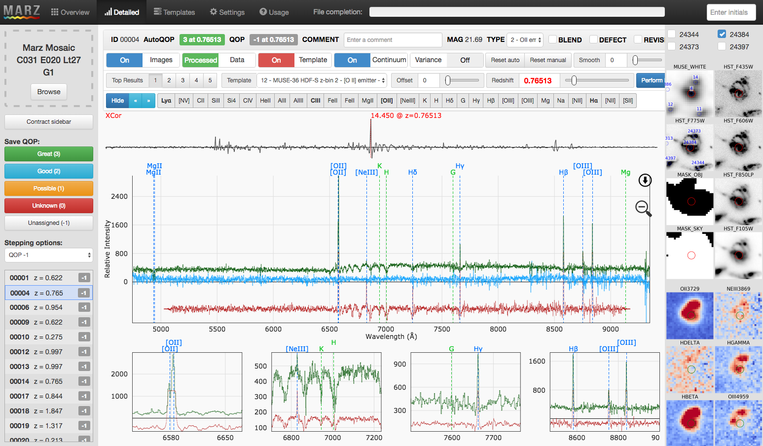
Figure 1: Redshift tool MARZ with some modifications for our redshift analysis. This tool reports the most likely redshift and the quality (QOP) by cross-correlating with input spectral templates. The redshift identifiers verify the suggested redshift or manually find a better redshift and provide its quality (indicated as CONFID in the catalogs). We also implement a feature to show images in the panel on the right.

The input spectral templates for MARZ are listed and explained in Appendix B. Some of the templates ($\rm No.\,6-19$) are made using the MUSE data. During the redshift identification process, no photometric redshift information is provided to the inspectors to avoid biases when we compare MUSE determined redshift against photometric redshift (Paper III). Instead, we display all of the existing HST UV to near-infrared images as supplemental information to the MUSE spectra. Although it is not yet implemented in our modified MARZ, we found that HST color images also help constrain spectroscopic redshifts and identify the corresponding object that is associated with the determined redshift.

For each of the determined redshifts, a confidence level (CONFID) from 3 to 1 is assigned:

• Secure redshift, determined by multiple features

• Secure redshift, determined by a single feature

• Possible redshift, determined by a single feature whose spectral identification remains uncertain

Although we identified emission and absorption features in the one-dimensional spectra, we employed narrowband images of the features to confirm the significance of the detections. The CONFID is assigned only when the identified features are seen in its narrowband images. The redshifts with CONFID of 2 or 3 are reliable, but if one is interested in using the redshifts with CONFID of 1, it is highly recommended to double check the spectrum and use it with care.

While measuring redshifts, we kept records of which feature is mainly used for the identification. This parameter is saved as the integer, TYPE, corresponding to

• Star

• Nearby emission line object

• [O ii] emitter

• Absorption line galaxy

• C iii] emitter

• [O iii] emitter

• Ly$\alpha$ emitter

• Other types

In general, the most prominent feature is used to define the type. We distinguished nearby galaxies (1) and [O ii] emitters (2) by a detection of H$\alpha$. Thanks to the relatively high spectral resolution of MUSE, it is possible to distinguish the [O ii] $\lambda\lambda 3726,3729$ and C iii] $\lambda\lambda 1907,1909$ doublet features based on their intrinsic separations at a certain redshift. It also helps to resolve the distinctive asymmetric profile of Ly$\alpha$. We discuss this further in §4, but the majority of redshifts are determined by identifying the most prominent feature, the [O ii] and Ly$\alpha$ emission at low redshift ($z<1.5$), and high redshift ($z>3$), respectively. Galaxies are only classified as [O iii] emitters when [O iii] is more prominent than [O ii] in cases both are detected.

We also kept the information of the data quality with the parameter DEFECT. The default is $\rm DEFECT=0$, meaning no problem is found in the data. When $\rm DEFECT=1$, it indicates that there are some issues with the data, but the data are still usable. This flag is raised often owing to the object lying at the edge of the survey area. This may indicate that line fluxes of these sources are underestimated because they are truncated in the data. As long as a spectral feature can be identified, we are able to determine a redshift, but we cannot recover the total line fluxes beyond the edge of the survey area.

For each continuum detected object, at least three investigators independently assessed the redshift. For udf-10, because it is our reference field, we had six investigators look at all of the objects. For the mosaic, $1147$ objects ($\rm F775W\leq 27$ mag, see Section 3.1.1) are divided equally for two groups with three investigators each. In the case of the emission line detected objects, two investigators individually determined redshift for all of these objects for both udf-10 and the mosaic. For both continuum and emission line detected objects, among each of the groups, any disagreements in their determinations of redshift, CONFID, TYPE, and DEFECT were consolidated to provide a single set of redshift results. With the consolidated results, we had at least one more person, who is not in the group, check all of the determined redshifts and related parameters to finalize the redshift assessment.

Then we refined the redshift by simultaneously fitting all of the detected emission lines and measure line fluxes using a spectral fitting software. This process is discussed in the next subsection.

3.3 Line flux measurements

For the redshift determination, the spectra utilized were primarily extracted based on either the white-light or PSF weighted extraction in order to optimize S/N. For the purpose of cataloging line fluxes, we alternatively used the unweighted summed spectra for all of the sources within each segmentation map . This avoids possible biases introduced by the weighting scheme. It is also better when the spatial distribution of the line emission is more extended than the white-light emission or PSF. This is especially relevant for Ly$\alpha$ emission (cf. Wisotzki et al., 2016; Leclercq et al., 2017). However, this results in an increased scatter for faint emission lines.

For the detected emission lines with $\rm S/N>3$, the line flux and its uncertainty are provided along with the measured redshift in the released catalog (Appendix A). We used the spectral line fitting software PLATEFIT (Tremonti et al., 2004; Brinchmann et al., 2008) to simultaneously fit all of the emission lines falling within the spectral range. This tool first uses a set of model template spectra from Bruzual & Charlot (2003) with stellar spectra from MILES (Sánchez-Blázquez et al., 2006) to fit the continuum of the observed spectrum at a predefined redshift with strong emission lines masked. After subtracting the fitted continuum from the observed spectrum, a single Gaussian profile is fitted to each expected emission line in velocity space. The velocity offset (the velocity shift relative to the redshift of the galaxy) and velocity dispersion of all of the emission lines are tied to be the same. See Tremonti et al. (2004) for a more detailed description of the software.

The velocity offset is limited to vary within $\pm 300\,{\rm km\,s^{-1}}$. For emission line galaxies, we used the velocity offset output from PLATEFIT to refine the original (input) redshift. The calculation of the velocity offset includes Ly$\alpha$ when it is detected. The typical velocity offset is about $10$ km s^-1 on average. When the original redshift is obtained directly from MARZ’s cross-correlation, we do not expect the offset to be significant, but it can be larger when the redshift identifiers manually estimate the redshift.

As described above, PLATEFIT fits single Gaussian functions to the emission lines. However, this is not suitable for Ly$\alpha$ because it is often observed to have an asymmetric profile. Thus, we added a feature to the software to fit the complicated profile of Ly$\alpha$. Instead of fitting Ly$\alpha$ with a single Gaussian function, we used a combination of multiple Gaussian functions (up to 21, although typically much fewer are used) at fixed relative positions to fit the Ly$\alpha$ profile. We placed a central component Gaussian function at the position of Ly$\alpha$ as determined by the single Gaussian fitting carried out in the previous step. We placed an additional 10 components on either side of this, at a constant spacing of $120\,{\rm km\,s^{-1}}$ to be consistent with the spectral resolution of the data. As such the fitting covers a velocity range of $\pm 1200\,{\rm km\,s^{-1}}$ from the expected position of the line.

We then performed the minimization via a nonlinear least squares method. During this process, the fluxes of each Gaussian component are allowed to vary independently (with most falling to 0 as they lie in the spectrum where Ly$\alpha$ has no emission) until the aggregate of all components best matches the observed spectrum. The separation between each component is kept constant (in velocity) but the wavelength of the central component is allowed to shift ($\pm 300\,{\rm km\,s^{-1}}$, consistent with fits for other lines). This allows for the fitting to correct for small discrepancies in the central position determined during the multiple Gaussian component fitting so that it produces a more accurate fit to Ly$\alpha$. The widths of individual Gaussian components are forced to be the same but the width itself is a free parameter. The PLATEFIT tool places a limit of $<500\,{\rm km\,s^{-1}}$ for each line width, but in general the Gaussian components only vary slightly from the initial guess of $70\,{\rm km\,s^{-1}}$ and fall between $60$ and $120\,{\rm km\,s^{-1}}$. Allowing the widths of the components to vary in this way produces a better fit to the data in a few cases, compared to running the fitting with a single fixed width for all of the components. However, the improvement is much less significant than that obtained by allowing the central velocity of the components to shift.

After the fitting, we studied the output spectrum of the complex fitted regions and identified individual complex “lines” (a composite of multiple Gaussian components) by searching the fit spectrum for local maxima. The routine then scans out from each maxima on either side of the peak until it identifies a local minimum or the fitted spectrum returns to 0. The flux of each complex line is then calculated along with its associated error and fitted “lines” with a S/N of less than 3 are dropped. This S/N cut successfully avoids overfitting the noise and removes unphysical fits (such as more than two components or very broad components) in most cases. The properties of the remaining lines are then calculated directly from the fitted spectrum using a model independent approach. Errors are determined using a Monte Carlo method by modifying the input spectrum with random values within the associated errors at each point 100 times. Each line property is then re-extracted for each realization and the standard deviation of these values is given as the error. An example of the complex fitting is presented in Figure 2.

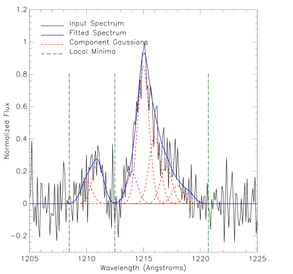
Figure 2: Demonstration of the complex fitting for a Ly$\alpha$ emission line presenting blue and red bumps. The fitting is performed on a simulated spectrum (black line) to better illustrate the procedure (the flux is in arbitrarily units). In the real data, the final fit is usually comprised of fewer components. The dashed red lines are the individual Gaussian components and the solid blue line is the total of these components (the final fit). The vertical green dashed lines indicate the local minima. We use the Ly$\alpha$ peak position to measure the redshift (see § 3.2).

3.4 Continuum flux measurements

Throughout the paper, we used the continuum fluxes from the HST observations provided in the UVUDF catalog. In addition to that, we measured our own continuum fluxes for the objects that are not in the UVUDF catalog but are identified by directly detecting their emission line features with ORIGIN and MUSELET (see §3.1.2). For these objects, we performed our own photometric measurements on the HST images to obtain segmentation maps and continuum fluxes or upper limits. A full analysis of why these objects are not in the UVUDF catalog and our method of extracting their broadband properties are described in Paper I. Here we provide a brief summary.

Among $160$ objects that are only found by ORIGIN/MUSELET, roughly one-quarter have very low or no continuum emission, and thus they are hardly detectable in any broadband images. The rest of the objects can be visually identified in the images, but they are not detected by SExtractor  (Bertin & Arnouts, 1996). In order to measure continuum fluxes (or upper limits) of these objects, we used NoiseChisel , which is an image analysis software employing a noise-based detection concept (Akhlaghi & Ichikawa, 2015). It is run independently on each of the HST images and the largest (from all the filters) object closer than $0.30\arcsec$ to the position reported by ORIGIN/MUSELET is taken as representing the pixels associated with it to create a segmentation map for each object. We are able to associate a NoiseChisel segmentation map for $76\%$ of the objects only found by ORIGIN/MUSELET. However, for the rest of the objects, no NoiseChisel segmentation map (in any of the HST broadband images) can be found within $0.30\arcsec$. For these objects, a $0.50\arcsec$ diameter circular aperture was placed on the position reported by ORIGIN/MUSELET.

The broadband magnitude is found by feeding the image of each filter and the final segmentation map into MakeCatalog, which takes output of NoiseChisel as input to directly create a catalog. The error in magnitude for each segment is derived from the S/N relation: $\sigma_{M}=2.5/(S/N\times\ln{(10)})$ (see Eq. (3) in Akhlaghi & Ichikawa, 2015). MakeCatalog produces upper limit magnitudes for each object, by randomly positioning its segment in $200$ different blank positions over each broadband image and using $3\sigma$ of the standard deviation of the resulting distribution. If the derived magnitude for an object in a filter is fainter than this upper limit, the upper limit magnitude is used instead.

4 Results

4.1 Redshift determination in the MUSE Ultra Deep Field (udf-10)

In this subsection, first we report the measured redshift and the parameters associated with it in our reference field, the MUSE Ultra Deep Field (udf-10). In addition to being the deepest spectroscopic field so far observed with MUSE, all of the extracted MUSE spectra in this field have been visually inspected. In the udf-10 field, as discussed in §3, we used two different procedures to extract the sources. Their redshifts were determined independently first, and then reconciled. Here we first present the basic properties of the objects associated with their redshift measurements for each extraction method independently. Based on our understanding of the differences and the relationship between the two source extraction methods and the redshift properties, we tried to find the best combination of these two methods to efficiently maximize the detection rate of redshifts in the even larger sample size of the MUSE Deep Field (the mosaic).

4.1.1 Redshifts of the continuum selected objects

Among $854$ continuum selected objects in the MUSE Ultra Deep Field (udf-10), we successfully measured the redshifts of $282$ objects in the redshift range from $z=0.21$ to $6.64$. The number of redshifts with confidence level $\geq 2$ is $223$.

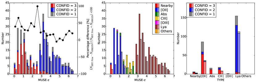
Figure 3: MUSE redshift distributions of the objects extracted with the HST continuum-detected priors (filled bars) and the direct line emission searches (ORIGIN; filled and faded color bars on the right in each bin) in the MUSE Ultra Deep Field (udf-10). All of the extracted sources are shown without removing overlaps between the extraction methods. [Left] The redshift histogram in bins of $\Delta z=0.35$. The red, blue, and gray represent the confidence levels 3, 2, and 1, respectively, for the determined redshifts. The filled dots show the percentage difference relative to the total of HST prior and ORIGIN MUSE-$z$ distributions. [Middle] The same redshift distribution as the left panel, but color coded by the classified type of the objects. [Right] The histogram of the classified type of the objects color coded by the redshift confidence levels.

In the left two panels of Figure 3, we show the distributions of redshifts found with the MUSE data. Because most of the objects at $0<z<1.5$ are usually identified by the [O ii] doublet, their CONFID is mostly 3 by definition when the double peaks are resolved and clearly seen. There are six cases in which CONFID is 2 in this redshift range, whose spectra in general have lower S/Ns but the features are obviously detected in narrowband images.

On the other hand, galaxies at $z>3$ are often found by a single feature Ly$\alpha$, which gives CONFID of 2. For the case of $\rm CONFID=3$ at $z>3$, the C iii] emission or UV absorption features, and in some rare cases He ii, are also discerned. The number of determined redshifts drops significantly at $1.5\lesssim z\lesssim 3.0$. This is a well-known “redshift desert”, where [O ii] shifts out from the red end of the spectral coverage, although Ly$\alpha$ is still too blue to be detected. With the deep data, we are able to recover some of the redshifts in this range by detecting C iii] emission and some absorption features (e.g., Fe ii).

There are also 59 redshifts with $\rm CONFID=1$. Their redshifts are difficult to determine with confidence, because in most cases, it is ambiguous to use their line profile to specify the feature (e.g., [O ii] versus Ly$\alpha$). For [O ii] emitter at $0.25<z<0.85$, H$\beta$ and [O iii] are in general also available, but they lie in a sky line crowded region, which can sometimes prevent further constraint on the measured redshift to give a higher CONFID.

4.1.2 Redshifts of the emission line selected objects

Of the $306$ emission line selected objects (objects detected with ORIGIN regardless of whether they have UVUDF counterparts), $154$ objects have secure redshift measurements with CONFID of 2 or 3 in the redshift range of $0.28-6.64$. When we include the $\rm CONFID=1$ redshifts, the resulting number of measured redshifts is $160$. Since we have to actually detect the emission features to select this sample, it is expected that the number fraction of $\rm CONFID=1$ redshifts is much smaller for the emission line selected objects compared with the continuum selected objects. A crucial difference between the continuum and line emission selected objects is that the former are extracted regardless of whether they are detected with MUSE or not, but the latter requires actual line detections.

The redshift distributions of the emission line objects are shown as the faded color bars (on the right in each bin) in Figure 3. Similar to the continuum selected objects, the majority of the redshifts at $z<3$ have $\rm CONFID=3$, while mostly $\rm CONFID=2$ at $z>3$, because of the detectable spectral features. The main features that ORIGIN detects to facilitate the redshift identifications are [O ii], Ly$\alpha$, and C iii]. The lack of redshifts in this range is more significant for the emission line selected objects because by nature ORIGIN does not have the ability to find any absorption galaxies.

4.1.3 Redshift comparisons between the continuum and emission line selected objects

When we only consider the secure redshifts ($\rm CONFID\geq 2$), the derived redshifts of both the continuum and emission line selected galaxies cover a similar range, from $z=0.2$ to $6.7$. A large difference is the numbers of identified redshifts between these two data sets. The continuum selected galaxies have $223$ secure redshifts, while the emission line selected galaxies have $154$. If we consider that of these $154$ objects, $30$ do not have a continuum detection (not in the prior list), the difference is even larger.

In the left panel of Figure 3, the percentage difference of the numbers of determined MUSE redshifts between the two extraction methods (HST prior or ORIGIN) is shown with the filled dots. The ORIGIN method is optimized to detect compact emission line objects with faint continuum, such that it is more sensitive to the detection of high-$z$ emission lines. This method misses $44\%$ of the [O ii] emitters identified in the continuum selected galaxies. For the Ly$\alpha$ emitters, $38\%$ of the continuum detected sample are not found by ORIGIN. There is no obvious trend of the fraction of missed [O ii] or Ly$\alpha$ with redshift (Figure 4). There is no trend found with line surface brightness either.

At $1.5<z<3$, the number of confirmed redshifts is smaller for the emission line selected galaxies because in this redshift range we mostly rely on galaxies with absorption features to find their redshifts in addition to C iii]. The ORIGIN method is not designed to detect absorption features, and thus it is not able to detect any of these objects. While the other feature, C iii], is in emission, it is fairly weak, which makes it harder for ORIGIN to detect. As shown in Figure 4, line fluxes of the C iii] emission not detected by ORIGIN are at the low end of the line fluxes. Although it is possible to tune ORIGIN to detect fainter emission features in the cube, it also dramatically increases the number of spurious detections.

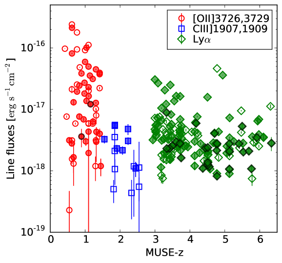
Figure 4: Line fluxes of [O ii] $\lambda\lambda 3726,3729$ (the red circles), C iii] $\lambda\lambda 1907,1909$ (the blue squares), and Ly$\alpha$ (the green diamonds) of the redshift-identified galaxies in udf-10 (CONFID $\geq 2$). The open and filled symbols are the HST continuum and emission line selected objects, respectively. The filled symbols with the black edge indicate that they are detected only by ORIGIN.

4.1.4 Final redshifts for the MUSE Ultra Deep Field (udf-10)

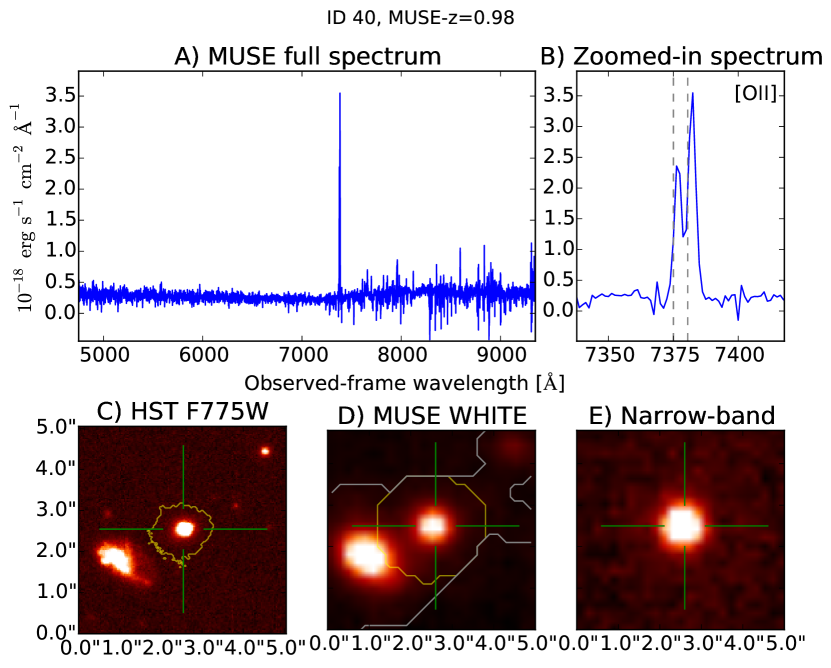
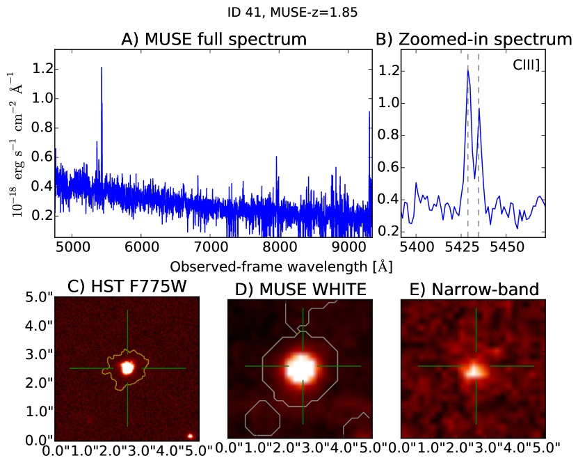
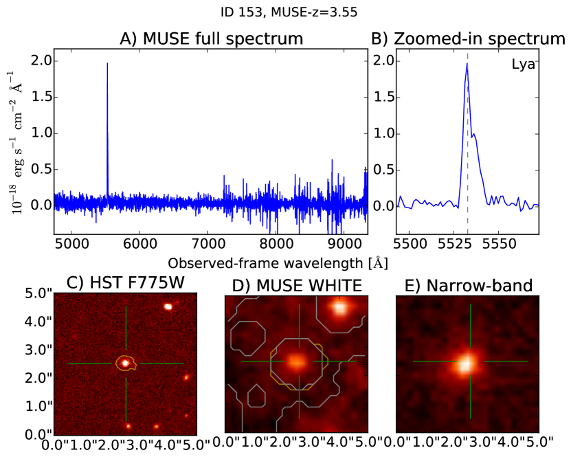
Figure 5: Full MUSE spectrum and a zoomed-in portion of the [O ii], C iii], and Ly$\alpha$ detected wavelength region at the top of each panel, and the HST F775W, MUSE white-light, and narrowband images of each emission line in the bottom of each panel. The yellow contours in the images are the boundary of the UVUDF catalog segmentation for the object, but those in the MUSE white-light image are convolved with the MUSE beam size. The white boundaries indicate masked objects excluded from local sky residual estimates. The green cross indicates the central position of the extracted object. The ID numbers and measured redshift are indicated at the top of each panel. All of these redshifts are secure ($\rm CONFID=2\,or\,3)$.

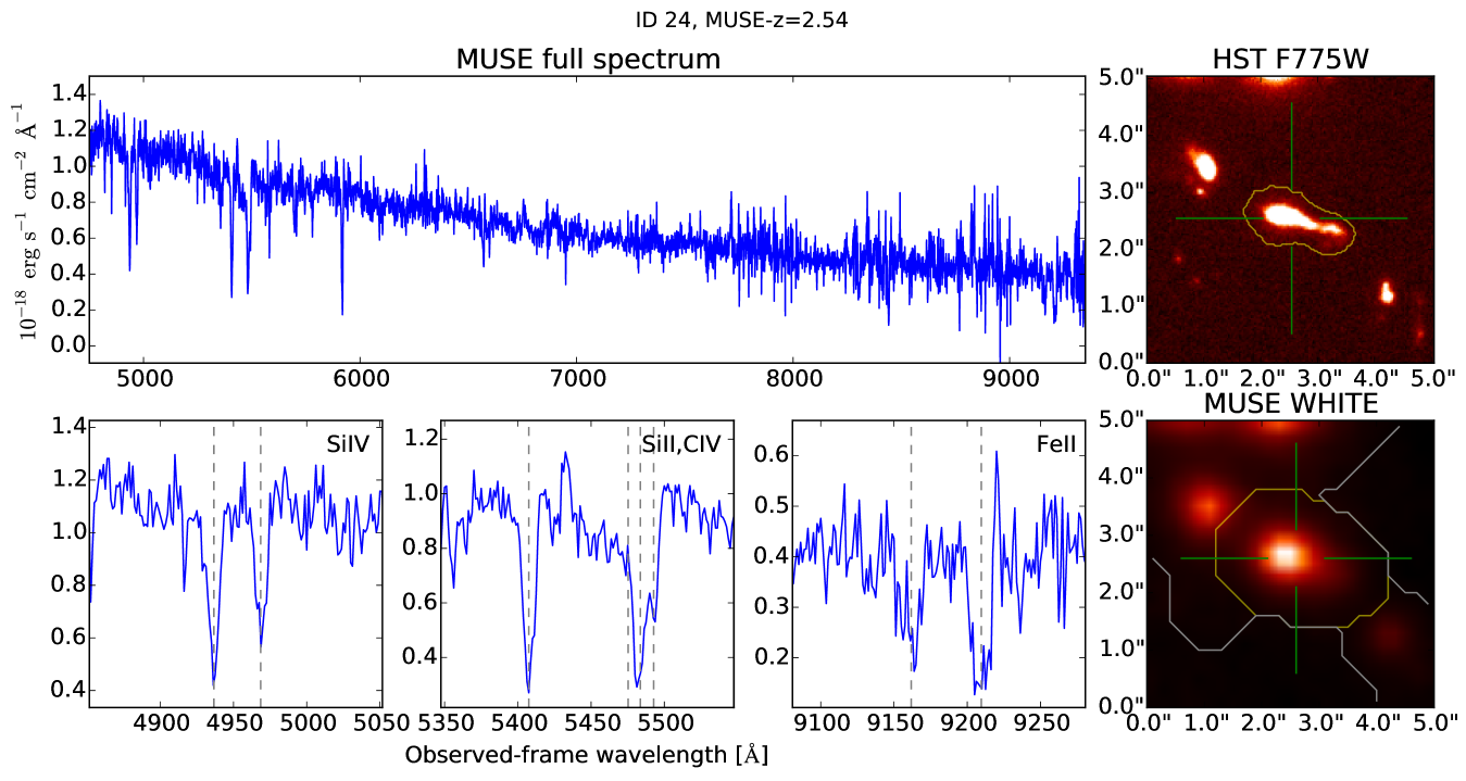
Figure 6: Full MUSE spectrum and a zoomed-in portion of the SiIV, SiII and CIV, and FeII absorption features. The HST F775W and the MUSE white-light images are shown on the right. The yellow contours in the images are the boundary of the UVUDF catalog segmentation for the object, but those in the MUSE white-light image are convolved with the MUSE beam size. The white boundaries indicate masked objects excluded from local sky residual estimates. The green cross indicates the central position of the extracted object. The ID number and measured redshift are indicated at the top.

We combined and compared the results from the independent measurements of the continuum and emission line selected objects to obtain the final redshifts. All of the determined redshifts are provided in the catalog (Appendix A). We show some example spectra and narrowband images of [O ii], C iii], and Ly$\alpha$ emitters, and an absorption line galaxy in Figures 5 and 6.

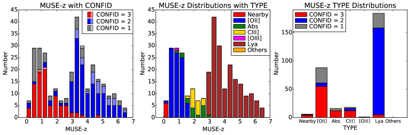
Figure 7: Final MUSE redshift distribution of the unique objects (i.e., overlapping objects are removed) combine both the continuum and emission line detected sources in the MUSE Ultra Deep Field (udf-10). [Left] The redshift histogram in bins of $\Delta z=0.35$. The red, blue, and gray colors represent the confidence levels 3, 2, and 1, respectively, for the determined redshift. The objects only found by ORIGIN are indicated by the faded colors, whereas in Fig. 3 all of the ORIGIN detected objects are shown. [Middle] The same redshift distribution as the left planel, but color coded by classified type of the objects. [Right] The histogram of the classified type of the objects color coded by the redshift confidence levels.

We successfully measured $313$ and $253$ redshifts with $\rm CONFID\geq 1$ and $\geq 2$, respectively, for the unique objects selected with the continuum or line emission (i.e., overlapping objects are removed). The final MUSE redshift distribution in udf-10 is shown in Figure 7 and summarized in Tables 8 and 9. The shape of the histogram does not change compared with the individual redshift assessments (Figure 3): two peaks at $z\approx 1$ and $z\approx 3$. The number of $\rm CONFID=2$ redshifts at $z\leq 1.5$ is $69$, at $1.5<z\leq 3$ (redshift desert) it is $29$, and at $3<z\leq 6.7$ it is $155$.

Table 1: Counts of determined redshifts for different source extractions in the MUSE Ultra Deep (udf-10), Deep field (mosaic), and the unique objects of udf-10 $+$ the mosaic

	udf-10 ($1\arcmin\times 1\arcmin$)			mosaic ($3\arcmin\times 3\arcmin$)			combined
Confidence level (CONFID)	$\geq 3$	$\geq 2$	$\geq 1$	$\geq 3$	$\geq 2$	$\geq 1$	$\geq 3$	$\geq 2$	$\geq 1$
HST continuum selected	$87$	$223$	$282$	$515$	$636$	$714$	$570$	$1206$	$1414$
With UVUDF counterparts				$547$	$1133$	$1295$
Emission line selected	$46$	$154$	$160$	$450$	$1057$	$1163$	$467$	$1112$	$1214$
Emission line only	$2$	$30$	$31$	$15$	$114$	$144$	$15$	$132$	$160$
Total unique objects	$89$	$253$	$313$	$562$	$1247$	$1439$	$585$	$1338$	$1574$

Table 2: Census of the objects in the MUSE Ultra Deep (udf-10) and Deep field (the mosaic) sorted by categories

	udf-10 ($1\arcmin\times 1\arcmin$)			mosaic ($3\arcmin\times 3\arcmin$)			combined
Category/Type	Counts	Redshift	F775W mag	Counts	Redshift	F775W mag	Counts
0. Stars	0 (0)	…	…	9 (1)	…	$19.0-24.8$	9 (1)
1. Nearby galaxies	5 (1)	$0.21-0.31$	$22.6-30.0$	47 (2)	$0.10-0.42$	$18.6-27.1$	47 (3)
2. [O ii] emitters	61 (27)	$0.33-1.45$	$20.4-28.8$	465 (49)	$0.28-1.49$	$19.4-28.3$	473 (73)
3. Absorption line galaxies	12 (4)	$0.95-3.00$	$21.9-26.1$	57 (22)	$0.60-2.95$	$21.0-26.2$	63 (23)
4. C iii] emitters	16 (2)	$1.55-2.54$	$23.8-29.8$	41 (18)	$1.55-2.86$	$23.4-27.0$	50 (18)
5. [O iii] emitters	1 (0)	$0.71$	$27.3$	2 (1)	$0.42-0.71$	$27.0-27.3$	2 (1)
6. Ly$\alpha$ emitters	158 (26)	$2.94-6.64$	$25.5-31.1+$	624 (97)	$2.91-6.63$	$24.4-31.2+$	692 (115)
7. Others	0 (1)	…	…	2 (2)	$1.22-3.19$	$21.0-24.6$	2 (2)

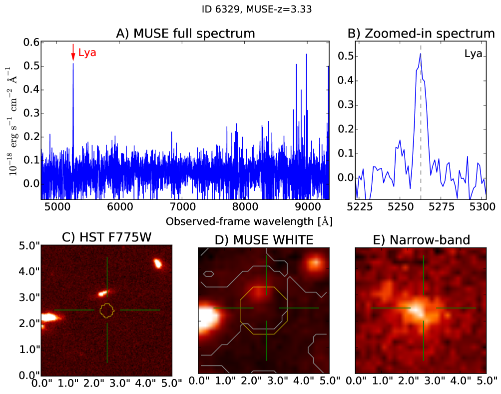
Figure 8: Example of an object that is not detected by continumm emission but found by ORIGIN. The full MUSE spectrum and zoomed-in part of the Ly$\alpha$ detected wavelength region are presented at the top. The HST F775W, MUSE white-light, and Ly$\alpha$ narrowband images are at the bottom.

In Figure 7, it is also immediately noticeable that beyond $z=3$, the fraction of confirmed redshifts of the objects detected only by ORIGIN (the faded color regions) increases. By $z\approx 6$, it reaches $\approx 50\%$. According to Figure 4, the ORIGIN detections do not seem to favor any specific redshift ranges or line fluxes (except of course when the line flux is below its detection limit). Two [OII] emitters ($\rm CONFID\geq 2$) were only detected by ORIGIN: MUSE ID 6314 and 6315. The disturbed morphology of ID 6314 in the HST imaging likely accounts for the no detection with SExtractor. The other object, ID 6315, is blended with a nearby bright source and are difficult to separate using solely imaging data. For the 28 Ly$\alpha$ emitters identified only by ORIGIN, most of these sources have surface brightness continuum emission that is too low to be detected with SExtractor (we measured $\approx 30$ mag with NoiseChisel) or are not visible by eye (Figure 8), but there are a small number of cases that are missed in the UVUDF catalog because of blending or because they are lying close to nearby bright sources (ID 6313) and disturbed/complex morphology in the HST images (ID 6324). We emphasize that these 28 objects represent $\sim 20\%$ of Ly$\alpha$ emitters found in this work and they are in a small $1\arcmin\times 1\arcmin$ area of the entire sky where the deepest HST data exist.

4.2 Redshift determination in the MUSE Deep Field (the mosaic)

4.2.1 Strategy based on the results in udf-10

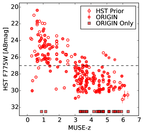
Figure 9: Magnitudes of HST F775W plotted against determined redshift ($\rm CONFID\geq 2$) for udf-10. The open and filled symbols represent the continuum (HST prior) and emission line (ORIGIN or MUSELET) extracted objects. The filled squares are the objects detected only with ORIGIN or MUSELET, and thus their F775W mags are upper limits. The horizontal dashed line indicates 27 mag where we make the cut to the continuum selected galaxies to perform the redshift determination in the mosaic field (see §4.2.1).

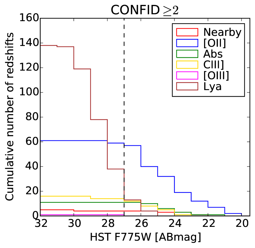
Figure 10: Cumulative counts of secure redshifts in udf-10. The colors indicate different types with the same scheme as in Figure 3.

Based on the redshift analysis in our deepest survey field udf-10, we tried to find the best combination of the two extraction methods to maximize the efficiency of redshift identifications. As shown in Figure 9, for the objects with redshift determined, 85 out of 98 objects at $z<3$ ($\rm CONFID\geq 2$), mostly [O ii] emitters, have $\rm F775W\leq 27$ mag (see also Figure 10). While the majority at $z>3$ are fainter than 27 mag, $106$ out of $155$ objects ($70\%$) in this redshift range are detected by line emission directly in the data cube with ORIGIN. In addition, all of the absorption galaxies, which ORIGIN cannot detect, are brighter than $26.1$ mag.

We simulated expected [O ii] line fluxes to investigate the sudden reduction of [O ii] emitters fainter than 27 mag visible in Figure 10. With the spectral energy distribution (SED) fitting code FAST  (Kriek et al., 2009), we used all of the galaxies in the mosaic with photo-$z$ (BPZ) of $0-1.5$ provided in the UVUDF catalog to predict their [O ii] fluxes. With the simple assumption that all of the [O ii] emission originates from star formation, we can directly translate the star formation rates obtained from SED fits of the HST photometry into expected [O ii] fluxes. Then we correct the [O ii] fluxes for dust extinction using the median dust correction factor, which is derived for the galaxies that are detected with MUSE using the Balmer decrement. The modeled [O ii] fluxes decrease with the F775W magnitude. From the $3\sigma$ line flux detection limit of the mosaic, $\approx 3\times 10^{-19}\,{\rm erg\,s^{-1}\,cm^{-2}}$, the fraction of detectable [O ii] emitters drastically decreases at $\rm F775W\gtrsim 27$ mag. At 27 mag, we expect $\approx 80\%$ of the [O ii] emitters to be detected, but it abruptly decreases to $\approx 20-50\%$ between $27-28$ mag. These numbers are likely to be upper limits because, for simplicity of the model, all galaxies are assumed to be star forming.

Thus, we make a cut at $\rm F775W\leq 27$ mag to limit the number of the continuum selected objects based on the HST priors for which we need to perform the visual inspection on redshift determination. This reduces the total number of $6288$ continuum selected objects to $1147$ to be inspected. For the emission line selected objects, we do not apply any preselection and examine all of the $1251$ spectra of the emission line detected objects.

In the near future, we plan to extend the redshift determination toward galaxies with $\rm F775W>27$ mag. At present, we only release the redshift measured in the $\rm F775W\leq 27$ mag continuum selected sample and all of the emission line selected sample as the first version of the MUSE UDF redshift catalog (Appendix A).

4.2.2 Redshifts in the mosaic

The process of the redshift evaluation in the mosaic follows the same procedure as udf-10. We inspected the continuum detected and emission line detected objects individually, and then reconciled these two objects to obtain the final redshifts.

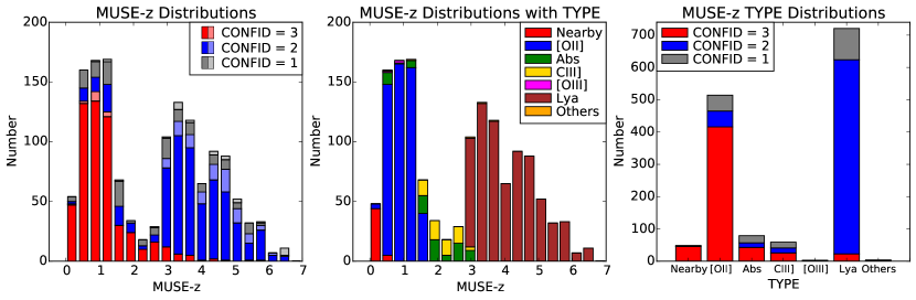
Figure 11: Same histograms as Figure 7 but for the MUSE Deep Field (the mosaic).

The summary and distributions of the determined redshifts are shown in Tables 8 and 9 and Figure 11. Out of the $1147$ continuum selected objects ($\rm F775W\leq 27$ mag), redshifts of $714$ and $636$ objects are determined with confidence levels of $\geq 1$ and $\geq 2$, respectively. When we include the emission line selected objects, these numbers increase to $1439$ and $1247$. Among these, $1295$ and $1133$ objects, respectively, have detectable UVUDF counterparts.

The fractions of the identified redshifts below and above $z=3$ are different compared with those in udf-10. Out of $1247$ redshifts with $\rm CONFID\geq 2$ in the mosaic, $52\%$ ($650$) are at $z\leq 3$ and $48\%$ ($597$) are at $3<z\leq 6.7$. Whereas, in udf-10, there are $39\%$ ($98$) and $61\%$ ($155$), respectively, out of $253$ redshifts with $\rm CONFID\geq 2$. A larger percentage of Ly$\alpha$ emitters are detected in the deeper data of udf-10 than in the mosaic, whose integration times are about three times different. This trend stays the same, even when we only account for the continuum detected objects (i.e., excluding the objects detected only by ORIGIN and MUSELET): $56\%$ ($631$) at $z\leq 3$ and $44\%$ ($502$) at $z>3$ for the mosaic, and $43\%$ ($96$) and $57\%$ ($127$), respectively, for udf-10. In addition, a smaller fraction of redshifts ($10\%$) is found in the “redshift desert” at $1.5<z\leq 3.0$ compared with udf-10 ($13\%$). These differences between the mosaic and udf-10, due to the depth of the data, are also implied by the higher fraction of $\rm CONFID=2$ redshifts at $z<3$ in the mosaic. Interestingly, the deeper data of the udf-10 increase the number fraction of $\rm CONFID=1$ redshifts in the [O ii] emitters compared to the mosaic. Among all of the determined [O ii] and Ly$\alpha$ emitters, the $\rm CONFID=1$ redshift is 11% and 16% of the $\rm CONFID\geq 2$ redshift, respectively, for the mosaic, while it is 44% and 16%, respectively, for udf-10. This is possibly because with higher S/N spectra, it is easier to find more features. The depth of the data also affects the detection rate of the ORIGIN/MUSELET-only objects at $z>3$. We do not see the same tendency as in udf-10, where the fraction of the determined redshifts of the ORIGIN/MUSELET-only objects to the continuum extracted objects increases with redshift. One nearby galaxy, 14 [O ii] emitters, and 99 Ly$\alpha$ emitters are found only by ORIGIN/MUSELET with $\rm CONFID\geq 2$ in the mosaic.

Thanks to the larger survey area of the mosaic, we find more rare objects than in udf-10. As an example, the one-dimensional spectrum of a quasar at $z=1.22$ (MUSE ID 872 or UVUDF ID 23796) with prominent Mg ii emission is shown in Figure 12 . This spectrum also exhibits Fe ii and Mg ii absorption features. These features only appear in the spectrum when it is extracted within the quasar PSF and are likely to be due to an intervening absorber at $z=0.98$ (cf. Rigby et al., 2002).

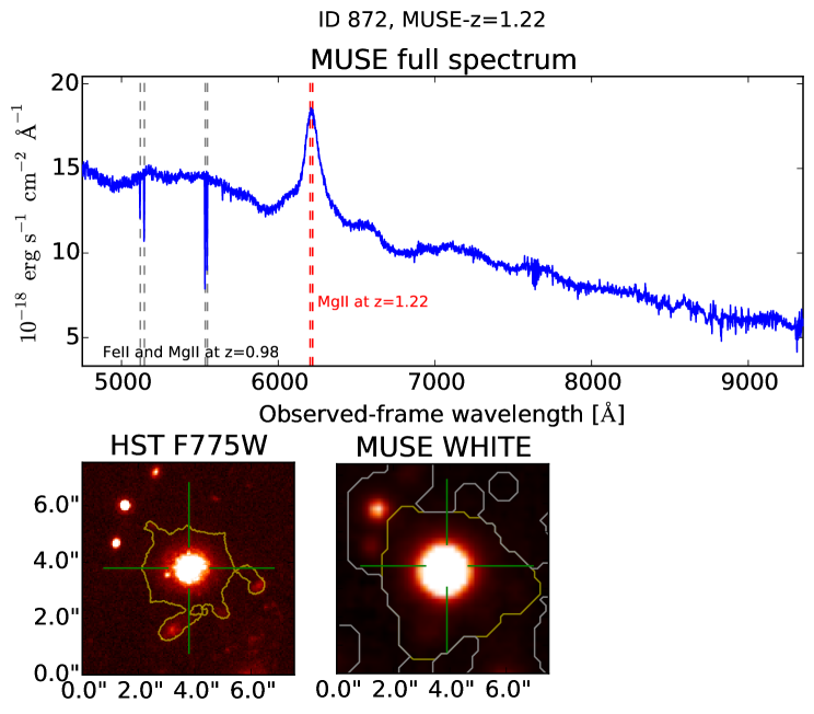
Figure 12: Full MUSE spectrum of a quasar at $z=1.22$ detected with a broad, prominent Mg ii emission feature. An intervening absorber (Fe ii and Mg ii) at $z=0.98$ is also detected. The cutout ($7.6\arcsec\times 7.6\arcsec$) for this object is larger than the standard $5\arcsec\times 5\arcsec$.

4.3 Redshift comparisons between the overlap region in MUSE Ultra Deep (udf-10) & Deep Field (the mosaic)

The mosaic redshift determination is performed independently from udf-10. In this subsection, we show direct comparisons of the measured redshifts and the associated parameters in the overlap region of these two fields.

In the overlapping part of the mosaic and udf-10 fields, all of the redshifts (regardless of CONFID) identified in the mosaic are also identified in udf-10 with the same CONFID or higher, except MUSE ID 275 and four objects detected only by ORIGIN or MUSELET (MUSE IDs 6432, 6447, 6865, and 7396). The redshift of ID 275 is measured to be $z=2.9$ in both udf-10 and the mosaic, but CONFID are 1 and 2, respectively. This is because the object lies at the edge of the udf-10 field, which gives less confidence. The four objects detected only by emission lines found in the mosaic data cube (with $\rm CONFID\geq 2$) are missed by the ORIGIN run in udf-10.

Among $313$ redshifts identified in udf-10, there are 13 redshifts that disagree with the redshifts identified in the mosaic by $|\Delta z|>0.01$. For the object discussed above, MUSE ID 275, the redshift is measured to be $z=2.899$ and $2.931$ in udf-10 and the mosaic, respectively. Apart from this object, one (MUSE ID 6684) has the same CONFID of 2 and four (MUSE IDs 44, 49, 90, 127) have the same CONFID of 1 in both udf-10 and the mosaic, but all of the rest (MUSE IDs 64, 103, 718, 6335, 6339, 6676, 6686) have the high CONFID of 2 or 3 in the udf-10 whereas CONFID of 1 in the mosaic. Below, we analyze why the obtained redshifts have differences (CONFID is given in the parentheses):

With the same CONFID

6684 $z_{\rm\textsf{udf-10}}=4.740$ (2), $z_{\rm\textsf{mosaic}}=0.871$ (2)

A clear emission feature is detected in both udf-10 and the mosaic, but it is identified as Ly$\alpha$ in udf-10 and as [O ii] in the mosaic. This is because the line profile in the mosaic spectrum shows double peaks (due to lower S/N) whose separation matches that of [O ii] at $z=0.871$. However, because this object is not detected in the UV imaging, it is more likely at higher redshift. Thus, we conclude that the feature is Ly$\alpha$ and its redshift should be $4.740$ as determined in udf-10.

44 $z_{\rm\textsf{udf-10}}=1.610$ (1), $z_{\rm\textsf{mosaic}}=1.436$ (1)

Both of the redshifts are from absorption features, but a set of multiple Fe ii absorption features are found in different wavelength regions. The CONFID for both of these redshifts are low.

49 $z_{\rm\textsf{udf-10}}=1.864$ (1), $z_{\rm\textsf{mosaic}}=1.578$ (1)

The Al iii and Fe ii absorptions are identified in udf-10, but a different set of absorptions are possibly seen in the mosaic. Owing to low S/N in the continua, they are both not certain.

90 $z_{\rm\textsf{udf-10}}=0.734$ (1), $z_{\rm\textsf{mosaic}}=2.389$ (1)

The same emission feature detected at $6465$${\rm\AA}$ in udf-10 and the mosaic is identified as [O ii] and C iii], respectively. With the low S/N data, it is difficult to confidently distinguish whether it is [O ii] or C iii].

127 $z_{\rm\textsf{udf-10}}=0.616$ (1), $z_{\rm\textsf{mosaic}}=4.035$ (1)

This is an interesting case in which different sets of emission features are spotted in the udf-10 and mosaic spectra. In udf-10, emission features at $6025$${\rm\AA}$, $7855$${\rm\AA}$, and $8090$${\rm\AA}$ are identified as [O ii], H$\beta$, and [O iii] 5007 at $z=0.616$. In contrast, none of these features are identified in the mosaic, but an emission line is identified at $6120$${\rm\AA}$. This feature is attributed to Ly$\alpha$. Reviewing the udf-10 spectrum, this feature is clearly detected. Thus, we think that there are probably two objects at $z=0.616$ and $z=4.035$ lying along the sightline. In the combined udf-10 and mosaic catalog, we use $z=0.616$ for ID 127 and add a new object with ID 7582 for the Ly$\alpha$ emitter at $z=4.035$.

Higher CONFID in udf-10

64 $z_{\rm\textsf{udf-10}}=1.847$ (2), $z_{\rm\textsf{mosaic}}=1.566$ (1)

The C iii] doublet is well detected at $5430$${\rm\AA}$ in udf-10. The mosaic redshift was measured by tentative absorption features. However, with a closer look, the same C iii] seen in udf-10 is weakly detected in the mosaic. Thus, the redshift of this object is likely to be $1.847$ as measured in udf-10.

103 $z_{\rm\textsf{udf-10}}=3.002$ (3), $z_{\rm\textsf{mosaic}}=2.986$ (1)

A clear Ly$\alpha$ absorption detected in both udf-10 and the mosaic spectra. In udf-10, there are also multiple UV absorption lines. Taking into account that the features used to determine the redshift are absorption and very broad, $|\Delta z|$ of 0.016 is not a significant difference. We use the udf-10 redshift as the final redshift.

718 $z_{\rm\textsf{udf-10}}=4.524$ (2), $z_{\rm\textsf{mosaic}}=0.801$ (1)

Similar to ID 6684, the spectrum of the mosaic is noisier than udf-10, which causes spurious double peaks of the identified emission feature. In the udf-10 spectrum, the feature shows a clear asymmetric profile with a red wing, indicating Ly$\alpha$. Thus, the redshift should be $4.524$ as in udf-10.

6335 $z_{\rm\textsf{udf-10}}=4.370$ (2), $z_{\rm\textsf{mosaic}}=1.098$ (1)

A clear emission feature is detected in udf-10 at $6525$${\rm\AA}$ whose profile indicates Ly$\alpha$, while the identified feature ([O ii]) in the mosaic is unclear. We do not see any obvious features around $6525$${\rm\AA}$ in the mosaic spectrum. This is not surprising because the line flux is $\approx 1\times 10^{-18}\,{\rm erg\,s^{-1}\,cm^{-2}}$, just around the $3\sigma$ detection limit of the mosaic.

6339 $z_{\rm\textsf{udf-10}}=5.131$ (2), $z_{\rm\textsf{mosaic}}=5.121$ (1)

The same emission feature is recognized as Ly$\alpha$. It looks as if the detected Ly$\alpha$ has a blue bump (which is likely to be sky residual) in the mosaic. The blue bump is used to determine redshift, causing a redshift difference of 0.01. However, this blue bump is not visible in the deeper data of udf-10. Using $z=5.131$ from udf-10 is reasonable.

6676 $z_{\rm\textsf{udf-10}}=3.723$ (2), $z_{\rm\textsf{mosaic}}=0.541$ (1)

The emission line clearly looks like Ly$\alpha$ in the udf-10 spectrum and the UV continuum emission is not detected. However, in the mosaic spectrum, although the same feature is identified, it is classified as [O ii]. Thus, the udf-10 redshift should be the correct one.

6686 $z_{\rm\textsf{udf-10}}=0.307$ (2), $z_{\rm\textsf{mosaic}}=4.383$ (1)

In the udf-10 spectrum, two emission features at $4875$${\rm\AA}$ and $6545$${\rm\AA}$ correspond to [O ii] and [O iii] 5007, which gives $z=0.307$. The former feature, in addition to not being convincing in udf-10, is not seen in the mosaic. The latter feature in the mosaic is recognized as Ly$\alpha$ because of its distinctive profile. This object is not detected up to the F435W band, which indicates that this object is likely to be at high redshift. Thus, the correct redshift is probably $z=4.383$ measured in the mosaic.

These results suggest that it is not necessary true that the success rate of CONFID in the shallower mosaic region is lower when comparing the same CONFID. We only found one case (ID 6684) in which the redshift in the mosaic field is not correct when both of the redshifts are $\rm CONFID=2$. When both redshifts are $\rm CONFID=1$ (IDs 44, 49 90, 127), their redshifts are too uncertain to make a judgement for the quality.

Because of the shallower depth of the mosaic, not all of the redshifts measured in udf-10 are found in the mosaic. Excluding the objects only found by ORIGIN/MUSELET, the mosaic misses 118 out of $282$ redshifts with $\rm CONFID\geq 1$ and 64 out of $223$ with $\rm CONFID\geq 2$ (night [O ii] emitters, six absorption line galaxies, six C iii] emitters, and 43 Ly$\alpha$ emitters). We only visually inspected the spectra of galaxies with $\rm F775W\leq 27$ mag and for the rest we relied on ORIGIN (and MUSELET). Thus, a subset of these missing redshifts may be recovered if we actually look at the spectra or change the tuning of ORIGIN (and MUSELET). If we include the objects that have no UVUDF counterpart (i.e., detected only by ORIGIN/MUSELET), then these numbers increase to 133 and 78 for $\rm CONFID\geq 1$ and $\geq 2$, respectively. The smaller number of ORIGIN/MUSELET detections in the overlap region in the mosaic can also be attributed to the depth of the data.

Together with this paper, we release both the udf-10 and mosaic redshift catalogs (Appendix A). As explained above, the ID numbers of the objects in the overlapping region are the same in udf-10 and the mosaic. In addition, we compiled a final redshift catalog combining the udf-10 and mosaic results. For the objects that have measurements from both of the catalogs, the information is from udf-10, unless there is a disagreement with the mosaic. For those cases, we adopted the redshifts discussed above. For the discussion below, we used the redshifts and the associated parameters from this combined catalog.

4.4 Final redshifts in the entire MUSE UDF survey region

In the entire MUSE UDF survey region (udf-10 $+$ the mosaic), there are $7904$ UVUDF sources that we used as priors to extract the continuum selected objects. As shown in Table 8, for $1206$ (15%) of them, we successfully obtained secure redshifts ($\rm CONFID\geq 2$). As discussed above, some of the objects were merged because of the lower spatial resolution of MUSE than HST and we did not investigate a subset ($\rm F775W\leq 27$ mag in the mosaic where not overlapping with udf-10) of their spectra to determine redshifts. The direct searches of emission line objects enabled us to find $132$ more redshifts in addition. Thus, in total, we obtained $1338$ unique redshifts with high confidence ($\rm CONFID\geq 2$). The final redshift distribution is presented in Figure 13. As a simple test, we compared the broadband (F775W) luminosity against the measured MUSE redshifts ($\rm CONFID\geq 2$) to check whether there are any catastrophic measured redshifts. This test does not show any extreme outliers.

We used the redshifts determined in both udf-10 and the mosaic to derive the distribution of redshift differences between these two catalogs. The standard deviation of the $\Delta z/(1+z)$ distribution is 0.00017. Assuming that the errors are similar for the udf-10 and mosaic redshifts (i.e., assuming that the depth of the data is not a dominant factor for redshift errors), then we obtain a global estimate of the redshift/velocity uncertainty to be $\sigma_{z}=0.00012(1+z)$ or $\sigma_{v}\approx 40\,{\rm km\,s^{-1}}$.

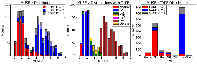
Figure 13: Same histograms as Figures 7 and 11, but for the combined redshifts of the unique objects from the MUSE Ultra Deep Field (udf-10) and MUSE Deep Field (the mosaic).

5 Discussion

5.1 Redshift measurement success rates

Assuming all of the determined redshifts are correct for $\rm CONFID\geq 2$, we calculated the success rates of the redshift measurements. Here we define the success rate as the number fraction of the obtained secure redshifts over the sample size we inspected. We only used the sample extracted with the HST priors for this calculation (i.e., the objects detected only by ORIGIN/MUSELET are excluded). In the mosaic, all galaxies with $\rm F775W>27$ mag are extracted by ORIGIN/MUSELET (or due to splitting; see §5.3). In other words, the success rates at $\rm F775W>27$ mag for the mosaic should be considered as lower limits.

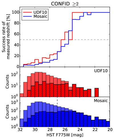
Figure 14: Success rates of obtained secure redshifts are shown in the top panel for udf-10 (red) and mosaic (blue). The horizontal dashed line indicates $50\%$ completeness. We only use the objects with HST counterparts in the UVUDF catalog in this plot (i.e., the objects detected only by ORIGIN/MUSELET are excluded). The middle and bottom panels show the counts of the total number of the HST objects (solid bars) and the MUSE redshift determined objects (hatched bars). The vertical dashed line in the bottom panel indicates the magnitude cut where we perform the redshift investigation on the continuum detected objects.

In Figure 14, the success rates of udf-10 and mosaic are plotted against the HST F775W magnitude. In udf-10, we successfully measured secure redshifts ($\rm CONFID\geq 2$) for all of the galaxies brighter than $25$ mag. At the same magnitude, the success rate for the mosaic is $87\%$. The $100\%$ success rate for the mosaic is at $<22.5$ mag (or $23.5$ mag if we ignore one object MUSE ID 6934 without MUSE redshift in the $22.5-23.0$ mag bin). The 50% completeness with respect to the HST F775W magnitude is reached at $26.5$ mag and $25.5$ mag, in udf-10 and the mosaic, respectively. The success rates decrease with the F775W magnitudes, in particular there is a sudden drop at $\approx 25$ mag for both of the fields. However, the success rate remains greater than $\approx 20\%$ at $<28-29$ mag in udf-10 and $\lesssim 27$ mag in the mosaic. Except in the $25.0-25.5$ mag bin, at all magnitudes, the udf-10 success rate is higher than the mosaic.

Another MUSE deep survey in the Hubble Deep Field South (HDFS; Bacon et al., 2015), whose coverage is also a single MUSE field of view as our udf-10 and has a similar depth ($27$ hours), reaches the $50\%$ completeness at $26$ mag in the HST F814W band. The achieved slightly higher completeness in udf-10 is a natural consequence of the better line flux detection limit, which results from the improved data reduction and analysis compared to the HDFS data cubes (Bacon et al., 2015).

The spectroscopic completeness and comparisons with photometric redshifts are discussed in Paper III.

5.2 Objects only detected by ORIGIN or MUSELET

Owing to its wide FoV IFU with high sensitivity, MUSE enables direct detection of emission line objects with very faint continuum emission, which are improbable to target with slit spectroscopy and inefficient to find with narrowband imaging. In the entire $3\arcmin\times 3\arcmin$ survey area, we discovered $132$ emission line detected objects with confident redshifts which are not on the HST prior list. In the deepest region ($1\arcmin\times 1\arcmin$ area of udf-10), this number is $30$. Among these $132$ emission line objects, the majority are Ly$\alpha$ emitters (117). The rest are [O ii] emitters (14) and a nearby galaxy (1). Some of these objects in fact can be visually identified in the images but are blended  (see §4.1.4). However, especially for the Ly$\alpha$ emitters, even when they can be visually identified, they have very low surface brightness or are not detected in the continuum. As mentioned in §3.4, we performed our own flux or upper limit measurements for these galaxies, but here we look into the most recent HST catalogs in more detail to investigate their properties.

Our prior list is based on the UVUDF catalog created by running ColorPro (a wrapper of SExtractor; Coe et al., 2006) with the detection image obtained by averaging four optical (F435W; F606W, F775W, F850LP) and four near-infrared (F105W, F125W, F140W, F160W) images (Rafelski et al., 2015). Except for the blended galaxies, the continuum of the MUSE emission line objects was still too faint to be originally detected in the combination of this deepest detection image.

We also checked if any of the emission line only objects are in the CANDELS  GOODS-S multiwavelength catalog (Guo et al., 2013), and identified 52 objects (one nearby object, eight [O ii] emitters, and 43 Ly$\alpha$ emitters) that have potential counterparts within $1^{\prime\prime}$. This does not immediately mean that they are the actual corresponding objects because some ORIGIN/MUSELET detected objects are completely blended with known objects or happen to lie on the same sightline. We inspected these objects one by one and found one nearby galaxy, seven [O ii] emitters, and one Ly$\alpha$ emitter that exist in the CANDELS catalog. For this Ly$\alpha$ emitter (MUSE ID 6343 or CANDELS ID 15913), based on the prospective Ly$\alpha$ in its MUSE spectrum, its redshift is determined to be $5.5$. However, its $U$ magnitude is 28.5 mag in the CANDELS catalog, which is not probable for a high-$z$ galaxy because of the Lyman break at 912Å. It is more likely that this Ly$\alpha$ emitter happens to lie on the same line of sight as this galaxy. The template-fitting technique, TFIT (Laidler et al., 2007), is utilized for the CANDELS catalog. The TFIT tool uses spatial positions and morphologies in a high-resolution image as the priors to fit objects in lower resolution images. Until objects cannot be resolved in the high-resolution image, it can further perform deblending in the lower resolution images even when object separations are $\lesssim 1.5$ times the PSF FWHM, which is the limit for SExtractor. Thus, some of these closely separated objects could not be deblended in the UVUDF catalog but were in CANDELS. In fact, the one [O ii] emitter (MUSE ID 6315) that is not in the CANDELS catalog is not resolved even with HST, and the 42 Ly$\alpha$ emitters are barely detected or not at all.

5.3 Blend and split of merged objects

During the redshift evaluation process, we found some cases in which we were able to split the merged MUSE objects (see §3.1.1). Comparisons between a detected emission line narrowband image and the HST image provide the spatial information of the corresponding HST counterpart of the emission line object. An example is shown in Figure 15. The object shown in the MUSE white image (the middle panel) is originally extracted as a merged object, which corresponds to two HST-detected objects with UVUDF IDs of 8147 and 8118. While these two objects are clearly resolved in the HST F775W image (the left panel), they are not resolved in the MUSE white image (the middle panel). We managed to associate the determined redshift (based on Ly$\alpha$) with one of the HST objects, UVUDF ID 8147, by creating a narrowband image of the detected Ly$\alpha$ at $z=3.67$ (the right panel). Although we cannot fully deblend the MUSE emission because of the limited spatial resolution, we can assign individual MUSE ID numbers for these objects using their UVUDF coordinates (“split”). This Ly$\alpha$ emitter is given MUSE ID 6290 and the other is 6749. This process does not increase or decrease the number of objects whose redshifts are successfully reported as identified in the earlier sections, unless both (or multiple) of the split objects show clear features that can be used to determine redshift.

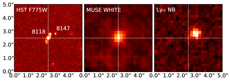
Figure 15: Stamp impage of $5\arcsec\times 5\arcsec$ centered at $\rm R.A.=53.169458$ and $\rm Dec=-27.778191$. The HST F775W image (white-light, left panel), the MUSE $\lambda$-collapsed image (middle), and the continuum subtracted narrowband image created at $\lambda=5676$${\rm\AA}$ with a width of $10$${\rm\AA}$ (right). While it is not possible to resolve the two nearby HST objects (UVUDF IDs of 8147 and 8118) with the MUSE white-light image, the combination of the HST image with the narrowband image of the detected emission line (Ly$\alpha$ in this case) makes it possible to identify the origin of the emission (UVUDF ID 8147 corresponds to MUSE ID 6290 with $z=3.67$).

Although small in number, there are also cases in which multiple redshifts are found in a single merged object. The MUSE IDs of 6877 and 6878 are originally merged and treated as a single MUSE extracted object. However, clear detections of the [O ii] doublet, [O iii] $\lambda\lambda 4959,5007$, and several Balmer lines at $z=0.734$ for ID 6877 and Ly$\alpha$ at $z=3.609$ for ID 6878 allow us to assign confident redshifts for both of the objects in addition to splitting them (Figure 16).

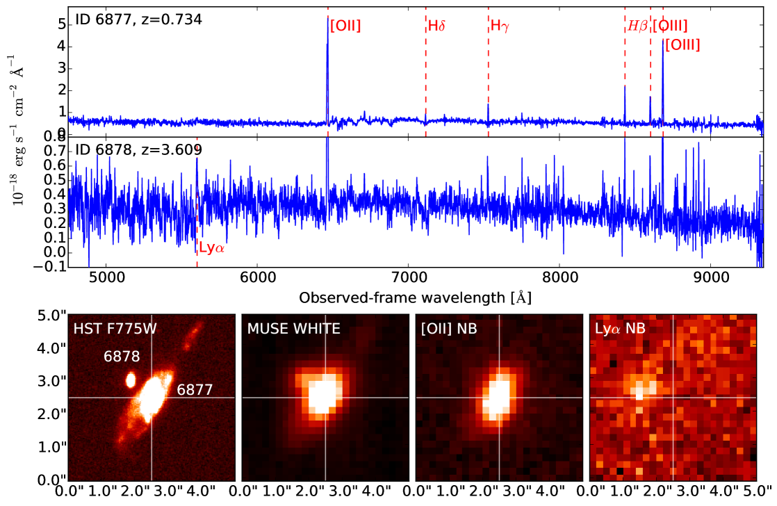
Figure 16: Spectra (extracted by PSF weighting) of MUSE IDs 6877 ($z=0.734$) and 6878 ($z=3.609$) at the top. The images shown at the bottom are HST F775W, MUSE white-light, and narrowband images of [O ii] at $z=0.734$ and Ly$\alpha$ at $z=3.609$, from left to right. Because these two objects are barely resolved with MUSE, they were originally treated as a single “merged” object. However, their spectra and a comparison of the narrowband images with the HST image help to “split” and associate the MUSE redshifts with the corresponding HST counterparts.

There are also some rare cases in which even though two or more of the merged objects have more than one redshift identified, they cannot be associated with any of the known objects owing to complex morphology, too close separation even for the HST, or no continuum detection. As shown in Figure 17, in the one-dimensional spectrum of an absorption galaxy at $z=2.575$, MUSE ID 942, multiple emission lines are visible at $7805$${\rm\AA}$, $8100$${\rm\AA}$, $8590$${\rm\AA}$, and $9090$${\rm\AA}$. These features do not correspond to any of the features that can be seen at $z=2.575$ of ID 942, but are consistent with [O ii], [Ne iii] $3869$, H$\delta$, and H$\gamma$ at $z=1.094$ (MUSE ID 7382), respectively. We use the center of the [O ii] narrowband image as the coordinates of this object. This particular case was found by hand, but ORIGIN has played an important role in finding these kinds of blended objects that are hard to find by humans. For example, multiple pronounced emission features seen in MUSE ID 945 immediately reveal its redshift to be $z=0.605$. It is very easy to neglect a weaker emission feature detected at $7230$${\rm\AA}$ in the same spectrum, which is not associated with ID 945. ORIGIN successfully found this feature and we identify it as Ly$\alpha$ at $z=4.947$ (MUSE ID 6470, no UVUDF counterpart).

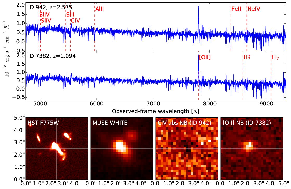
Figure 17: Similar to Figure 16, but for MUSE IDs 942 ($z=2.575$) and 7382 ($z=1.094$). The extracted spectra clearly show that there are at least two objects lying on the same sight line. A small offset is also seen between the narrowband images of the C iv absorption feature at $z=2.575$ and [O ii] at $z=1.094$. However, there is no obvious HST object to provide the counterpart for the [O ii] emitter.

In the end, we split about 150 of the merged objects. Among $1574$ objects with MUSE-$z$ ($\rm CONFID\geq 1$), there are 79 that remain as merged objects. We stress that we do not use or provide the photometric measurements for the merged objects. When merged objects have been successfully split during the redshift determination, the split objects have been associated with the corresponding photometries from the UVUDF catalog. If we find multiple redshifts in an object that is not merged (the case of Figure 17), only the object with the centroid in the narrowband images of the detected features closest to the UVUDF coordinates or the object with the reasonable HST color is assigned to have the UVUDF photometries.

5.4 Comparisons with previous spectroscopic redshifts

There has been a large effort to measure spectroscopic redshifts (spec-$z$) in the UDF and the surrounding regions, such as GOODS, VVDS, and VUDS. According to the list of spec-$z$ compiled in the UVUDF catalog by Rafelski et al. (2015) , there are $150$ previously known secure spec-$z$ in our survey region ($3^{\prime}\times 3^{\prime}$). The total number of published redshifts in the UVUDF catalog is 169 over the entire HUDF area. In addition, within a $0.5^{\prime\prime}$ search radius, we find that there are $11$ MUSE objects  that have previously known spec-$z$ measured by VUDS with high reliability (redshift flags of 4, 3, or 2; Tasca et al., 2017). Thus, in total, we compile $161$ previously known reliable spec-$z$ in our survey field. It is noteworthy that MUSE delivers a drastic improvement not only in the number of spec-$z$, but also in the range of redshift and the limiting magnitude of the objects with confident spec-$z$ (Figure 18).

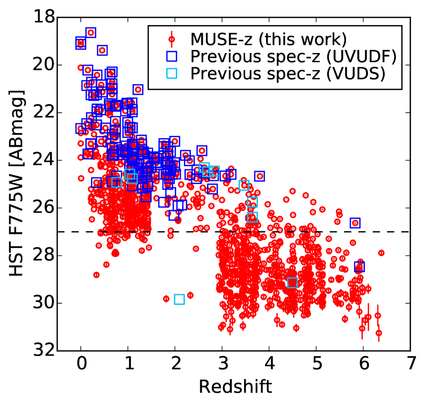
Figure 18: Magnitude vs. redshift space of secure MUSE-$z$ ($\rm CONFID\geq 2$; red circles) and previous reliable spec-$z$ for the unique objects in the entire MUSE deep survey region (udf-10 $+$ mosaic). The previously known spec-$z$ taken from the UVUDF and VUDS catalogs are indicated with blue and cyan squares, respectively. The horizontal dashed line indicates 27 mag where we make the cut to the continuum selected galaxies to perform the redshift determination in the mosaic field (see §4.2.1).

The majority (all for udf-10) of the published spec-$z$ are in the redshift range of $0<z<3$ and F775W magnitude of $<25$. The three objects at $z>3.5$ in the UVUDF catalog are from the spectroscopic observations of Lyman break galaxies (Vanzella et al., 2009) .

A simple check of MUSE redshifts is to compare them with the published spectroscopic redshifts. In Fig. 19, our MUSE spectroscopic redshifts are compared to these previously known spectroscopic redshifts. When we only use the robust redshifts (CONFID $\geq 2$), we find six objects with $|\Delta z|>0.01$ (MUSE IDs 29, 949, 957, 997, and 1048 from UVUDF and MUSE ID 6891 from VUDS), but all except IDs 997 and 6891 have $0.01<|\Delta z|<0.02,$ which is expected to happen owing to observations with different spectroscopic resolutions. We investigate the two objects with catastrophic differences below (CONFID of MUSE-$z$ is given in the parentheses):

997 $z_{\rm MUSE}=1.041$ (3), $z_{\rm known}=1.603$ (Morris et al., 2015)

The previous spec-$z$ is measured from WFC3 grism (G141) data by identifying H$\beta$ and [O iii] (with a good quality, 3 out of 4), while MUSE-$z$ is determined by a well-detected [O ii] doublet, [Ne iii] $3869$, H$\delta$, and H$\gamma$ (with CONFID of 3, the highest). Reinspecting the WFC3 grism spectrum verifies that $z=1.603$ is not as convincing as originally determined. In addition, there is an extra complication in extracting the grism slitless spectrum due to multiple nearby objects. Thus, we conclude that our MUSE redshift is likely to be correct for MUSE ID 997 (UVUDF ID 8592).

6891 $z_{\rm MUSE}=0.227$ (3), $z_{\rm known}=3.647$ (Tasca et al., 2017)

Although the redshift of ID 6891 (UVUDF ID 4864) is identified by good detections of H$\beta$, [O iii], and H$\alpha$, its spectrum is blended with ID 6892 (UVUDF ID 4863), which shows a Ly$\alpha$ emission line at $z_{\rm MUSE}=3.648$ ($\rm CONFID=2$). The separation of these two objects is $0.3^{\prime\prime}$. The previously measured spec-$z$ corresponds to MUSE ID 6892, but the pointing coordinates are closer to MUSE ID 6891. Also, these two objects were not successfully deblended in the CANDELS catalog (CANDELS ID 13745 for both of the objects). Thus, we think that our MUSE redshift measurement for MUSE ID 6891 (and 6892) has no problem.

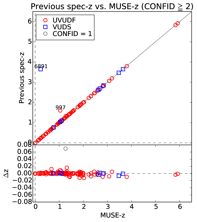
Figure 19: Comparisons of MUSE-$z$ to the previous spectroscopic redshifts from the other ground- and space-based telescopes compiled in the UVUDF catalog. The high and low confidence MUSE-$z$ are shown as red and gray symbols, respectively. MUSE ID 997 indicated in the figure is the only object with a catastrophic difference in the spec-$z$ comparisons. See the text for more details.

When including $\rm CONFID=1$ redshifts, one MUSE object (MUSE ID 1143) has previously known spectroscopic redshifts but disagrees with our MUSE redshifts ($z_{\rm MUSE}=1.262$ and $z_{\rm known}=1.332$ from Morris et al., 2015). The previously known redshift 1.332 is measured in the near-infrared spectrum obtained with HST/WFC3 grism (G141) spectroscopy. Morris et al. (2015) identified H$\beta$ and [O iii]. In our MUSE spectrum, we identified [O ii] $\lambda 3729$ at $8435$${\rm\AA}$, which gives $z=1.262$. Its CONFID is 1 because [O ii] $\lambda 3726$ is not detected probably because it overlies a sky line. The difference in redshift is $\delta z=0.07,$ which cannot be explained by the low spectral resolution ($R\sim 130$) of the grism spectroscopy. We found that the 3D-HST survey (Brammer et al., 2012) also published a redshift for this object of $z=1.299$ (by identifying H$\alpha$; Momcheva et al., 2016), which is consistent with our measurement. The slight discrepancy ($|\Delta z|=0.037$) can be attributed to the fact that the object is spatially extended in the dispersion direction for the grism. Thus, we assessed that the MUSE redshift for this object is more feasible.

There are 10 objects whose spec-$z$ are reported in the UVUDF (seven objects) and VUDS (three objects) catalogs but are missed by our redshift determination. These objects are listed below with MUSE ID, UVUDF ID in the parentheses, previously measured spec-$z$, and the reference:

55 (24380): $z=1.39\pm 0.01$ (Daddi et al., 2005)

The spectrum was obtained with HST/ACS grism low-resolution spectroscopy (G800L, $R\approx 100$ at $8000$${\rm\AA}$ for a point source), which detected a broad Mg ii absorption line. This feature is not seen in our MUSE spectrum even with smoothing probably due to much higher noise level in the continuum. This object is located in the overlapping region of the mosaic and udf-10, but we cannot find a redshift from the spectrum extracted from the deeper udf-10 data.

1199 (3482): $z=1.91\pm 0.01$ (Daddi et al., 2005)

Daddi et al. (2005) found a broad blended Mg ii $\lambda\lambda 2796,2803$ doublet absorption feature (and likely the Fe ii multiplet absorption) in their spectrum taken with HST/ACS grism spectroscopy. This feature can be identified in our MUSE spectrum too, but only after knowing the redshift or heavily smoothing the spectrum.

1308 (10544): $z=1.313$ (Morris et al., 2015)

The known redshift was determined using the spectrum taken with HST/WFC3 grism spectroscopy (G141, $R\approx 130$ at $1.1\leq\lambda\,{\rm[\mu m]}\leq 1.7$). The emission features H$\beta$, [O iii], and H$\alpha$ were identified to obtain $z=1.313$. With this redshift, we confirm the [O ii] emission at $8630$${\rm\AA}$ in our MUSE spectrum. It is located in the wavelength region where sky emission dominates, which made it easily missed during our redshift determination process. This redshift is added into the combined catalog by hand ($z_{\rm MUSE}=1.315$ with $\rm CONFID=3$).

1312 (21773): $z=1.76\pm 0.02$ (Daddi et al., 2005)

The HST/ACS grism spectrum detected a broad Mg ii absorption line. With the previously determined redshift, we can confirm the same feature in the MUSE data. However, it lies in a wavelength region crowded with sky lines, which makes it even harder to identify the feature without the a priori information.

1351 (4562): $z=2.145$ (Balestra et al., 2010)

The spectrum was taken with VLT/VIMOS. The previously known redshift was determined based on the O i ($1302.20$${\rm\AA}$) and C ii ($1335.10$${\rm\AA}$) absorption features detected at $4095$${\rm\AA}$ and $4200$${\rm\AA}$, respectively. These features are both outside the MUSE wavelength coverage, preventing us from recovering its redshift with MUSE. At this redshift, C iii] and some absorption features are covered by the MUSE wavelength range, but none of these features are visible.

1364 (8292): $z=2.067$ (Morris et al., 2015)

The redshift was measured in the spectrum taken with the HST/WFC3 near-infrared grism. These authors detected H$\beta$ and [O iii]. We can indeed recognize the Mg ii $\lambda\lambda 2796,2803$ absorption lines (and possibly Fe ii $\lambda 2344$ and Fe ii $\lambda\lambda 2374,2382$) in the MUSE data with this redshift. It is difficult to notice these features in our data because at this redshift, the Mg ii features lie in the low S/N region due to many sky lines.

1520 (21730): $z=1.98\pm 0.02$ (Daddi et al., 2005)

A broad Mg ii absorption feature (and possibly the Fe ii multiplet absorption) was detected in their HST/ACS grism spectrum. This feature might be visible in the MUSE data, but is not obvious because of crowded sky lines. It is difficult to use our MUSE data solely to determine this redshift.

4070 (635): $z=4.498$ ($z_{\rm flag}=3$) (Tasca et al., 2017)

The VUDS redshift (VUDS ID 532000222) may have been determined by a tentative Ly$\alpha$ emission at 6685${\rm\AA}$. In our MUSE spectrum we also discern an emission line at 6685${\rm\AA}$, but this is contamination from MUSE ID 1185 (Ly$\alpha$ at $z_{\rm MUSE}=4.50$), which is $2.38^{\prime\prime}$ away. It is possible that the VUDS slit also covered the extended Ly$\alpha$ emission from ID 1185, which led to $z=4.498$.

5216 (8384): $z=2.095$ ($z_{\rm flag}=2$) (Tasca et al., 2017)

It looks as though the VUDS redshift (VUDS ID 539990803) was derived from a good cross-correlation signal. However, our cross-correlation with MARZ does not provide a good signal and we are not able to find the expected absorption features at this redshift in our MUSE spectrum.

5494 (7285,7374): $z=0.768$ ($z_{\rm flag}=3$) (Tasca et al., 2017)

At the VUDS redshift (VUDS ID 532000256), we might expect to detect Fe ii, Mg ii, H$\beta$, and [O iii] in the MUSE spectrum, but none of these features are seen. The VUDS redshift is likely obtained through a good cross-correlation signal, but we are not able to do so with the MARZ cross-correlation.

Of these 10 redshifts that were missed by our redshift determination process, four were obtained via ground-based spectroscopy. However, for one of these redshifts (MUSE ID 1351), the detected features are not accessible with MUSE, and for the other three, we cannot confirm the previously measured redshifts in the MUSE spectra (IDs 4070, 5216, and 5494). The rest were taken with sky emission free space-based spectroscopy. The four optical spectra (HST/ACS) provide much higher sensitivity, especially in the continua, which facilitates detections of absorption features (Mg ii in this case). An extremely broad feature is also easily washed out in our higher resolution spectra without smoothing. The remaining two redshifts were measured with the near-infrared spectra from space (HST/WFC3). We can confirm the expected features in the MUSE spectra with the known redshift, although they are difficult to identify because their wavelengths are in the region of many strong sky emission lines.

5.5 Comparisons with photometric redshifts

We compared our MUSE determined spec-$z$ against the published photometric redshifts (photo-$z$) from Rafelski et al. (2015) in Figure 20. The merged objects (extracted with HST priors that cannot be resolved by MUSE) are not included in the plots. Rafelski et al. (2015) provide two sets of photo-$z$, based on the Bayesian photometric redshift (BPZ) estimation (Benítez, 2000) and the EAZY software (Brammer et al., 2008).

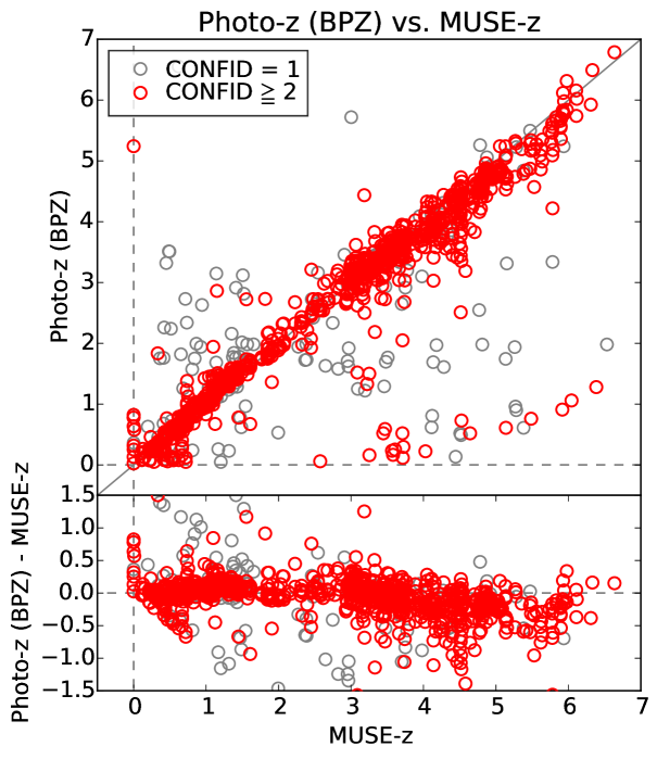
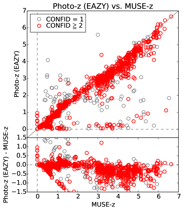
Figure 20: Comparisons of redshifts measured from the MUSE data in udf-10 $+$ mosaic compared with photometric redshifts, computed with BPZ (left) and EAZY (right). The redshifts with $\rm CONFID\geq 2$ and $\rm CONFID=1$ are plotted with the red and gray circles, respectively.

Although MUSE spec-$z$ and photo-$z$ agree well with both BPZ and EAZY up to $z\approx 3$, a systematic difference appears at $z\gtrsim 3$. Both of the photo-$z$ measurements tend to underestimate the redshift. All of the MUSE redshifts at $z>3$ are identified by Ly$\alpha$, which is known to cause the apparent offset toward higher redshift (of a few hundred $\rm km\,s^{-1}$; Shapley et al., 2003; Steidel et al., 2010; Hashimoto et al., 2013) attributed to galactic-scale outflows or absorption by the intergalactic medium. However, this Ly$\alpha$ apparent offset is not the major cause of the photo-$z$ offset because the median of the measured offsets ($\Delta z$) between MUSE-$z$ ($\rm CONFID\geq 2$) and photo-$z$ is significantly larger than the expected Ly$\alpha$ velocity offset ($\approx-0.13$ and $\approx-0.32$ for BPZ and EAZY, respectively). In Figure 21, the redshift difference is plotted against the HST F775W magnitude. It is clear that the photo-$z$ measurements are biased at the faint end.

Further analyses and discussions including the redshift completeness can be found in Paper III. In this paper, we checked the catastrophic redshift outliers and systematic biases. We found that changes in model of treatments of inter-galactic medium (IGM) absorption for Ly$\alpha$-forest and Lyman continuum absorption can reduce the photo-$z$ and MUSE-$z$ discrepancy. We also adopted photometric redshifts from the BEAGLE software (Chevallard & Charlot, 2016).

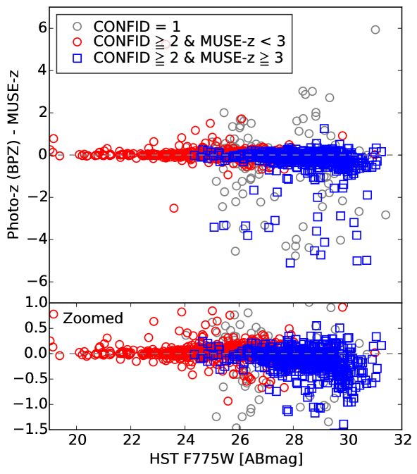
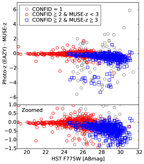
Figure 21: Difference in the photometric redshift and MUSE redshift (udf-10 $+$ mosaic) against the F775W magnitude. The redshifts with $\rm CONFID=1$ are plotted with gray circles. The secure redshifts ($\rm CONFID\geq 2$) are separated into two groups: $z<3$ (red circles) and $z\geq 3$ (blue squares).

5.6 Color selections of high-z galaxies

The presence of the 912${\rm\AA}$ Lyman break enables selection of high-redshift galaxies using their colors. Here we compared MUSE-$z$ to some commonly used color-color selection diagrams to discuss the fraction of successful color selections. The combination of the MUSE wavelength coverage and the HST filter sets observed in our deep field facilitates some tests on the color selection technique of $2\lesssim z\lesssim 6$ candidate galaxies. Known stars are excluded from all of these plots.

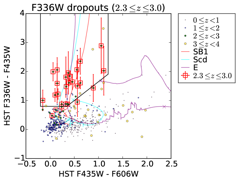
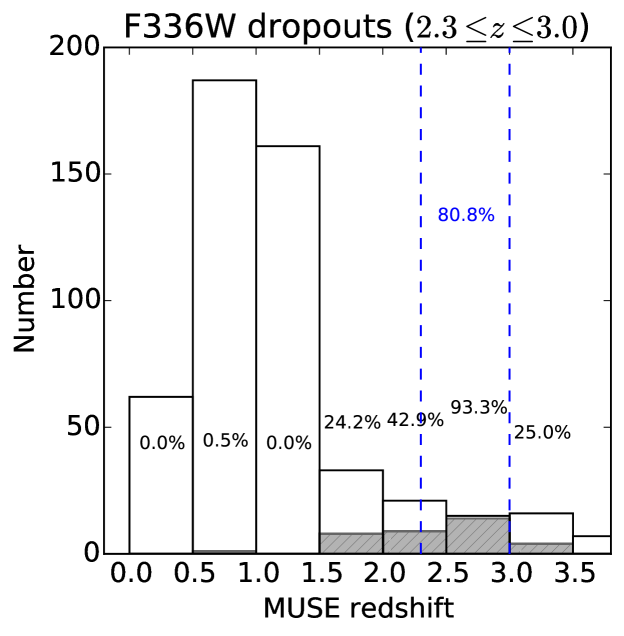
Figure 22: [Left] Color-color diagram of $F336W-F435W$ vs. $F435W-F606W$ to select $z\sim 2.7$ galaxies (F336W dropouts). Only the MUSE spectroscopic redshifts with $\rm CONFID\geq 2$ are plotted. The galaxies in the targeted redshift range ($2.3\leq z\leq 3.0$) are shown with red open squares. The violet, blue, green, gold, orange, magenta, and red filled circles, with sizes from small to large, indicate galaxies in $0\leq z<4$ with steps of $\Delta z=1$, respectively. The model tracks of the starburst template (SB1; Kinney et al., 1996) and the CWW templates (Scd and E, Coleman et al., 1980) are overlaid. The crosses on the model tracks indicate redshifts from $z=0$ in increments of $\Delta z=1$. [Right] The counts of galaxies in each redshift bin (only the galaxies detected in all of the F336W, F435W, and F606W bands are used here). The empty bars are all of the galaxies with MUSE redshifts and the filled bars are a subset of the MUSE redshifts lying within the F336W dropout selection boundary (the left panel). The percentages shown above each bar are the fractions of the galaxies within the color-color boundary for each bin. The vertical dashed blue lines indicate the targeted redshift range, $2.3\leq z\leq 3.0$. The percentage indicated in between these lines in blue is the fraction of the galaxies within the color-color boundary for the targeted redshift range.

In Figure 22 (left panel), we overplot all of the MUSE-$z$ on the F336W dropout selection diagram ($\rm F336W-F435W$ versus $\rm F435W-F606W$). The bandwidth of F336W favors Lyman break galaxies (LBGs) at $2.3\lesssim z\lesssim 3.0$. Although Hathi et al. (2010) and Teplitz et al. (2013) also show the F225W and F275W dropout selections, we exclude these from this paper because they preferentially select $z\sim 1.7$ and $z\sim 2.1$, respectively, which is a range in which MUSE does not recover a large number of redshifts. We follow the selection criteria of Hathi et al. (2010), i.e.,

F336W dropouts:

$$\begin{cases}&{\rm F336W-F435W>0.8}\\ &{\rm F435W-F606W<1.2}\\ &{\rm F435W-F606W>-0.2}\\ &{\rm F336W-F435W>0.35+[1.3\times(F435W-F606W)]}\end{cases}$$

The original selection conditions also apply a magnitude cut of ${\rm F435W\leq 26.5}$ mag and S/N limits of ${\rm S/N(F435W)>3}$, ${\rm S/N(F336W)<3}$, ${\rm S/N(F275W)<1}$, and ${\rm S/N(F225W)<1}$ to securely find high-$z$ candidates. We do not adopt these limits because our purpose here is to demonstrate where our galaxies with measured redshift lie in the diagrams. However, we do require solid detections, and thus no limit is shown in the diagrams.

The fraction of galaxies that meet these selection criteria in each redshift bin is shown in the right panel of Figure 22. This plot indeed identifies galaxies at $2.3\lesssim z\lesssim 3.0$ among the galaxies with secure redshift ($81\%$). If we limit to $2.5<z<3.0$, $93\%$ of the galaxies in this redshift range are classified as F336W dropouts. Those missed (the filled green circles in the left panel of Figure 22) lie very close to the selection boundary where lower-$z$ galaxies start to get intermingled, in particular around $\rm 0.5\lesssim F336W-F435W\lesssim 0.8$ and $\rm-0.2\lesssim F435W-F606W\lesssim 0.4$. There is only one interloper from galaxies at $0\leq z<1$ at $\rm F336W-F435W=0.93$ and $\rm F435W-F606W=0.27$, almost on the borderline. This object is MUSE ID 2537 ($z=0.717$) whose redshift is identified by H$\delta$ and [O iii] $\lambda\lambda 4959,5007$.

For even higher redshifts, we utilize the F435W, F606W, and F775W dropout techniques to inspect $z\sim 3.5$, $z\sim 5.0$, and $z\sim 6.0$ galaxy selections, respectively (Stark et al., 2009, 2010), as shown in Figure 23. The selection boundaries are listed below. Again, here we do not include any S/N cuts on the dropout conditions.

F435W dropouts:

$$\begin{cases}&{\rm F435W-F606W>1.1}\\ &{\rm F606W-F850LP<1.6}\\ &{\rm F435W-F606W>1.1+F606W-F850LP}\end{cases}$$

F606W dropouts:

$$\begin{cases}&{\rm F606W-F775W>1.2}\\ &{\rm F775W-F850LP<1.3}\\ &{\rm F606W-F775W>1.47+(F775W-F850LP)\leavevmode\nobreak\ or\leavevmode\nobreak\ 2.0}\end{cases}$$

F775W dropouts:

$$\begin{cases}&{\rm F775W-F850LP>1.3}\end{cases}$$

In all of these dropout selections, the targeted dropout galaxies are well captured. No low-$z$ interloper is found in any of these selections. The fraction of galaxies that lie within the boundaries is much smaller compared the F336W selection (Figure 24). This fraction also decreases from the lower-$z$ to higher-$z$ dropout selections ($41\%$, $34\%$, and $22\%$ for the F435W, F606, and F775W dropouts, respectively). If we limit the redshift bin to $3.5<z<4.0$, which is the most sensitive redshift range for the F435W filter to detect the dropouts, then $81\%$ of galaxies in this redshift bin meet the dropout criteria. Similarly, for selecting F606W and F775W dropouts, the fractions are highest ($67\%$ for both) in the redshift bins of $5.0<z<5.5$ and $6.0<z<6.5$. Although error bars are not shown in the diagrams (in order to make them readable), the errors of the objects outside of the selection boundaries are almost always smaller than those in the boundaries. Their positions are reliable in the color-color planes.

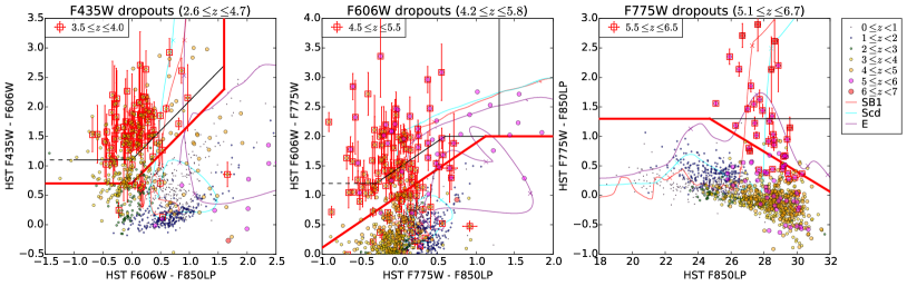
Figure 23: Similar to the left panel of Figure 22 but selecting $z\sim 3.5$ (F435W dropouts), $z\sim 5.0$ (F606W dropouts), and $z\sim 6.0$ (F775W dropouts), shown in the left, middle, and right panels, respectively. For the F435W and F606W dropouts, we do not plot the objects at $z>5.0$ and $z>6.0$, respectively. The galaxies indicated with the red squares are not in the full targeted redshift range, but are restricted to narrower ranges (see also Figure 24). The solid and dashed black lines are the boundaries of the selection criteria from Stark et al. (2009, 2010). The dashed black lines are shown because they are at the outside of the plotting regions in Stark et al. (2009, 2010). The solid red lines are our empirically redefined new selection boundaries to gain more galaxies in the targeted redshift ranges. The model tracks for the F850LP magnitude in the F775W dropout diagram is computed for an absolute magnitude of $-22$ mag. The 5$\sigma$ limit of the F850LP magnitude is 28.9 mag (Rafelski et al., 2015).

Figure 24: Similar to the right panel of Figure 22 but for investigating the fractions of galaxies that meet the dropout conditions at $z\sim 3.5$, $z\sim 5.0$, and $z\sim 6.0$, shown in the left, middle, and right panels, respectively.

From these results, we can empirically adjust the selection boundary to increase the fraction of the candidate galaxies at the targeted redshift ranges. Based on visual modifications, we relax the selection conditions based on our MUSE redshifts as follows:

Redefined F435W dropouts from MUSE-$z$:

$$\begin{cases}&{\rm F435W-F606W>0.7}\\ &{\rm F606W-F850LP<1.6}\\ &{\rm F435W-F606W>0.7+F606W-F850LP}\\ \end{cases}$$

Redefined F606W dropouts from MUSE-$z$:

$$\begin{cases}&{\rm F606W-F775W>1.0+0.89\times(F775W-F850LP)\leavevmode\nobreak\ or\leavevmode\nobreak\ 2.0}\\ \end{cases}$$

Redefined F775W dropouts from MUSE-$z$:

$$\begin{cases}&{\rm F775W-F850LP>-0.17\times F850LP+5.5\leavevmode\nobreak\ or\leavevmode\nobreak\ 1.3}\\ \end{cases}$$

These updated boundaries are shown with the solid red lines in Figure 23. The histograms of the selected galaxies with these new criteria are shown in Figure 25. We are trying this experiment, but not all of our sample galaxies in the diagrams (in particular those lying between the original and new boundaries) necessarily show a clear Lyman break because we only use Ly$\alpha$ emission to determine their redshifts.

Figure 25: Same plots as Figure 24, but for our empirically redefined new selection boundaries shown in Figure 23 with the red lines.

We allow a slightly bluer $\rm F435W-F606W$ color for selecting $z\sim 3$ galaxies (F435W dropouts) because there is a crowd of $3\leq z<4$ galaxies lying right below the original boundary. The new boundary significantly improves the $z\sim 3$ galaxy selection without picking up contaminants. In particular, now it finds $\approx 40\%$ more galaxies at $3.0<z<3.5$.

For the F606W dropouts, the targeted $z\sim 5$ galaxies also extend toward bluer $\rm F606W-F775W$ colors. Thus, we lower the color limit of $\rm F606W-F775W$. In addition, we remove the border at $\rm F775W-F850LP=1.3$ because some of galaxies at $5.5<z<6.0$ have redder colors. These new conditions successfully increase the fraction of $z\sim 5$ galaxies lying within the boundary from $34\%$ to $59\%$ and now capture $88\%$ of the galaxies in the $5.0<z<5.5$ bin and $66\%$ in the $4.5<z<5.0$ bin. This also adds one low-$z$ interloper and two galaxies at $3.0<z<4.0$ .

It is more difficult to enhance the $z\sim 6$ galaxy selection. We double the number of galaxies at $5\lesssim z\lesssim 6.5$ to meet the new conditions, but this also increases the number of galaxies at lower redshifts. With the newly suggested criteria, we cover galaxies at $6.0<z<6.5$ well ($83\%$) and improve a lot for galaxies at $5.5<z<6.0$ (from $29\%$ to $63\%$). There are more galaxies below $z=5$ in the new selection box, but only one is below $z=1$ (MUSE ID 2478 $z=0.73$). The remaining eight lower-$z$ galaxies have redshifts between $3$ and $5$. In total, we successfully select 29 galaxies at $5.0<z<6.5$. It is challenging to purely select galaxies at $5.0<z<5.5$ with this color-magnitude diagram because galaxies at $3<z<5$ have similar colors and magnitudes. We only collect two galaxies ($5.3\%$) in this bin using the new diagram (0 in the original one).

There are still significant numbers of high-$z$ galaxies lying outside of the selection boxes. We have checked these galaxies individually to determine whether their bluer colors are due to blending or photometric issues. In the F435W dropout diagram, we find 10 objects with $3.5\leq z\leq 4.0$ for $\rm F435W-F606W<0.9$. Among these objects, one may be blended with a nearby object, one is a dusty galaxy (ID 6672, see Figure 26) and one may have an ambiguous Ly$\alpha$ feature. In the remaining seven objects, two have good photometries lying near the revised selection box, and five have $S/N{\rm(F435W)}<5$ but the error budgets of their photometries make them agree with the revised selection box. For the F606W dropout diagram, we checked 12 galaxies with $4.5\leq z\leq 5.5$ for $\rm 0\lesssim F606W-F775W\lesssim 0.4$. There is one (ID 6324, Figure 26) whose photometries may be contaminated by a neighboring object, but the rest of the objects have good photometries (seven with $S/N{\rm(F606W)}\gtrsim 5$ and four with $S/N{\rm(F606W)}>10$; e.g., ID 2727, Figure 26). However, we find that all of these objects have the Ly$\alpha$ emission line lying in the F606W coverage, which is likely to produce bluer $\rm F606W-F775W$ colors. This effect is visible in the diagrams in Figures 25 and 24. Allowing the boundary of $\rm F606W-F775W$ to be bluer increases more lower-z selections in the targeted redshift range of $4.2<z<5.8$. In fact, this trend is also seen in the 13 outlier galaxies with $5.5\leq z\leq 6.5$ for $\rm 0\lesssim F775W-F850LP\lesssim 0.5$ in the F775W dropout diagram (e.g., ID 3238, Figure 26). All of these galaxies have $S/N{\rm(F775W)}\gtrsim 5$ and the detected Ly$\alpha$ line is lying in the F775W coverage; three of these galaxies are starting to enter the F850LP coverage, but at the wavelength where the F850LP filter throughput is still $<50\%$. Similar to the outliers in the F606W dropout diagram, the enhanced blue $\rm F775W-F850LP$ colors of these objects can be ascribed to Ly$\alpha$ emission contributing to the F775W flux. The newly defined selection boundaries help to increase the completeness of $3\lesssim z\lesssim 7$ galaxy selections. It is not surprising that we find outliers as color selection criteria are not designed for comprehensive detection. Although rest-frame UV spectra of high-$z$ galaxies are affected by IGM transmission, the high equivalent width of Ly$\alpha$ emission also causes bluer colors, which makes the apparent Ly$\alpha$ break less significant (particularly in the F606W and F775W dropout selections). In addition, color selections are known to exclude some high-$z$ passive and dust-obscured galaxies (e.g., Daddi et al., 2004; Reddy et al., 2005; van Dokkum et al., 2006). The outliers in the dropout diagrams are also found in the VVDS survey (Le Fèvre et al., 2005; Paltani et al., 2007).

Here we limit to the comparisons of measured redshifts against the dropout selections. The galaxy populations plotted here are likely to be different from the traditional dropout selected galaxies because the majority of the redshifts are determined with emission lines. However, candidate galaxies lying between the original and new selection conditions may be able to serve as second highest priority targets for multi-object spectroscopy to increase the efficiency in finding high-$z$ galaxies. Also, we do not adopt any S/N or magnitude cuts here. For future work, we will discuss in more detail why some galaxies fail to meet the dropout conditions (with respect to their spectroscopic and photometric redshifts), the relationship between Ly$\alpha$ emitters and dropout galaxies and their physical properties, and the evolution of the fraction of Ly$\alpha$ emitters.

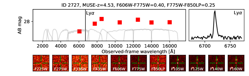
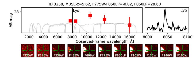
Figure 26: Examples of the outliers in the F435W (top panel), F606W (two middle panels), and F775W (bottom panel) dropout selections. In each panel, a spectral energy distribution using the HST photometries is shown at the top left, a zoomed-in part of the Ly$\alpha$ detected wavelength region is presented at the top right, and thumbnail HST images of the object are shown at the bottom. The object ID, MUSE spec-$z$, and the colors of each galaxy can be found at the top of each panel.

6 Summary and conclusions

We have conducted a deep spectroscopic survey in the HUDF with MUSE. The $3\arcmin\times 3\arcmin$ deep survey ($\approx 10$ hour depth, the mosaic) region almost covers the entire HUDF with the $1\arcmin\times 1\arcmin$ ultra deep survey ($\approx 30$ hour depth, udf-10) region enclosed. We used two different spectral extraction methods for the redshift identification: the HST prior continuum selected objects (based on the UVUDF catalog; Rafelski et al., 2015) and the emission line objects selected directly in the cubes without prior information. We visually inspected these spectra to determine redshifts via redshift analysis software. We also measured the line fluxes for the objects with redshifts determined. Along with this paper, we release the redshift and line flux catalogs. Here we summarize our findings in the redshift assessments:

1. In udf-10, we obtained $253$ secure redshifts ($\rm CONFID\geq 2$) in the redshift range $0.21\leq z\leq 6.64$. Among these, $30$ are not in the HST UVUDF catalog that we used for the prior based source extraction. The majority of these redshifts (28) are Ly$\alpha$ emitters. When we only count HST prior extracted objects, we managed to retrieve $223$ redshifts out of $854$ continuum selected objects ($26\%$). We reach a $50\%$ completeness at $26.5$ mag (F775W), and the completeness stays around $20\%$ up to $28-29$ mag.

2. In the mosaic, in addition to investigating all of the emission line galaxies, we performed visual inspections for those with $\rm F775W\leq 27$ mag for the continuum selected galaxies. This arbitrary cut is made based on our findings for udf-10 that $\approx 90\%$ of galaxies at $z<3$ are brighter than this magnitude. At $z>3$, although most of the galaxies are fainter than $27$ mag, we are able to detect $70\%$ of these galaxies with emission features directly in the data cube without any continuum information. Together with the direct search for emission line objects in the cube, this helps to increase the efficiency of redshift determination.

3. Out of the $1147$ continuum selected objects with $\rm F775W\leq 27$ mag in the mosaic field, we determined secure redshift of $636$ objects. When we included the emission line detected objects (regardless of magnitude), we obtained $1247$ unique redshifts with confidence. The $50\%$ completeness with respect to F775W mag is at $25.5$ mag.

4. In the overlapping region of udf-10 and mosaic, all of the redshifts measured in mosaic were also measured in the udf-10 with at least the same confidence level or higher, except one object lying at the edge of the udf-10 field and four objects detected only through emission lines in the mosaic cube. On the other hand, 78 secure redshifts were missing in mosaic when compared with udf-10. There are a few discrepancies but the measurements in the udf-10, which has higher S/N spectra, are usually more convincing.

5. Among $7904$ unique continuum selected galaxies in the entire MUSE UDF survey region (udf-10 $+$ the mosaic), we recovered redshifts for $1206$ (15%) objects. We also found $132$ objects only via emission line searches directly in the data cubes (no counterparts in the HST UVUDF catalog). Thus, in total, we obtained $1338$ unique redshifts with high confidence.

6. Compared with the HST beamsize, the MUSE data suffer from source confusion. However, we were able to partly solve this issue when an emission/absorption feature is identified. The location of the detected feature in its narrowband image can be associated with the location of the corresponding source in the HST images. There are also a few cases where two (or more) galaxies are completely blended even with the HST resolution, but we identified both (or all) of these cases with two (or more) different sets of emission lines at different redshifts. Finally, among $1574$ objects with MUSE-$z$ ($\rm CONFID\geq 1$), there are 79 that remain as merged objects.

7. Of the previously known $161$ spectroscopic redshifts in our survey field, we recovered all except 10 objects. Of these, four were measured in spectra taken with ground-based spectroscopy. However, for one of these redshifts, the detected features are at wavelengths shorter than the blue end of MUSE, and for the other three, we cannot confirm the previously measured redshifts based on the expected detectable features. The other six spectra were taken with HST grism spectroscopy. The features used for determining their redshifts either were a very broad absorption feature or lay on the red side of MUSE spectra where sky emission dominates.

8. The comparison of MUSE-$z$ and photometric redshifts revealed that they agree well up to $z\approx 3$. At higher redshift, an offset appears. Although most of the $z>3$ redshifts are determined with Ly$\alpha$, the median offset between MUSE-$z$ and photo-$z$ is much larger than the expected Ly$\alpha$ velocity offset to the systematic redshift due to gas motion. We observed a trend that the photo-$z$ offset increases with fainter continuum emission in HST/F775W.

9. We investigated all of the galaxies with secure MUSE-$z$ in some common color selection (dropout) diagrams of high-$z$ galaxies. With the F336W dropout selection criteria, $81\%$ of targeted $z\sim 2.7$ galaxies are captured. This fraction decreases for higher-$z$ selections: $41\%$ for F435W dropouts ($z\sim 3$), $34\%$ for F606 dropouts ($z\sim 5$), and $22\%$ for F775W dropouts ($z\sim 6$). We empirically redefined the selection boundaries to increase the fractions to $68\%$, $59\%$, and $45\%$, but our galaxy populations are likely to be different from the traditional dropout selected galaxies (continuum selected) because the majority of the redshifts were determined using emission lines.

With deep MUSE spectroscopic observations in HUDF, we dramatically improve the redshift completeness. The improvements are not only the increase in number from $161$ to $1338$, but also the coverage of the redshift range well beyond $z>3$ and depths up to the 30th magnitude (F775W). Together with existing large telescopes and planned future observatories such as JWST and 30 m class telescopes, it opens new horizons for exploring the early universe.

In the near future, we plan further advances in the analysis, such as investigating spectra extracted at the positions of continuum selected objects fainter than $27$ mag in the mosaic, fine tuning ORIGIN (and MUSELET) to further improve the direct detection of emission lines without enhancing spurious sources, upgrading MARZ to increase the accuracy of automated redshift determinations with newly built spectral templates, and developing deblending techniques based on prior information.

Appendix A MUSE UDF redshift catalogs

Along with this paper, we release the MUSE ultra deep field (udf-10) and deep field (mosaic) redshift and line flux catalogs. Because the udf-10 field is within the mosaic field, there is some overlap in the object entries. The combined catalog, which only includes a single set of redshift and the associated parameters (CONFID, TYPE, and DEFECT, and measurements in detected lines) for each unique galaxy, is also provided. For the cases with conflicting redshifts, we give the redshift discussed in §4.3, otherwise the udf-10 redshifts and the associated parameters are employed. In the Table 18, we describe the contents in the catalogs.

The UVUDF ID numbers are stored as strings (CSV) instead of integer numbers because some of the UVUDF objects are unresolved with MUSE and are merged to be treated as a single object (see Section 3.1.1). In order to find an object with the object ID from the UVUDF catalog, users can use the following commands in both Python 2 and 3:

from astropy.table import Table
import numpy as np

# Read catalog
>>> catalog = Table.read("catalog.fits", format="fits")

# Convert the catalog UVUDF_ID column to the string type
>>> UVUDF_IDs = catalog["UVUDF_ID"].astype(str)

# The UVUDF ID to search
>>> search_UVUDF_ID = "9525"

# Find the index number of the above UVUDF ID in the catalog
>>> idx = np.where(np.char.count(UVUDF_IDs, search_UVUDF_ID))[0][0]

# Print the above UVUDF ID and
#  its corresponding MUSE ID and the index number in the catalog
>>> print_format = "UVUDF ID={0} is MUSE ID={1} (UVUDF ID {2}) at index={3}"
>>> print(print_format.format(search_UVUDF_ID, catalog["MUSE_ID"][idx], UVUDF_IDs[idx], idx))

UVUDF ID=9525 is MUSE ID=70 (UVUDF ID 9525,9515) at index=61

Table 3: Column description of the redshift catalogs for the MUSE Hubble Ultra Deep Field (udf-10, mosaic, and combined)

No.	Title	Description
1	MUSE_ID	MUSE object identification number
2	RA	R.A. (J2000) in units of decimal degrees
3	DEC	Decl. (J2000) in units of decimal degrees
4	MERGED	Flag (boolean) indicating a merged object
5	UVUDF_ID	UVUDF object identification number (Rafelski et al., 2015)
6	ORIG_ID	ORIGIN object identification number
7	ORIG_RA	ORIGIN R.A. (J2000) in units of decimal degrees
8	ORIG_DEC	ORIGIN Decl. (J2000) in units of decimal degrees
9	MLET_ID	MUSELET object identification number
10	MLET_RA	MUSELET R.A. (J2000) in units of decimal degrees
11	MLET_DEC	MUSELET Decl. (J2000) in units of decimal degrees
12	EML_ONLY	Flag (boolean) for the objects detected only by ORIGIN or MUSELET (i.e., no UVUDF counterpart)
13	REF_SPEC	The main spectrum (PSF-weighted or MUSE white-light weighted) used to measure redshift
14	Z_MUSE	Spectroscopic redshift determined with MUSE
15	CONFID	Confidence level of Z_MUSE
16	TYPE	Type of feature used to identified Z_MUSE
17	DEFECT	Flag (0 or 1) indicating defect in the data (0 for no defect and 1 for some issues with the data)
18	F775W_MAG	HST F775W magnitude (AB) from Rafelski et al. (2015)   or NoiseChisel
19	F775W_MAG_ERR	The errors on the HST F775W magnitude (AB)
20-41	[LINE]_FLUX	Line fluxes ($\rm 10^{-20}\,erg\,s^{-1}cm^{-2}$) summed over the entire mask aperture   (see §3.3)
	[LINE]_FLUX_ERR	Errors on the line fluxes
Columns that only exist in the combined catalog
45	Z_FROM	The origin of the redshift (the udf-10 or the mosaic catalog)
46	IN_UDF10	Flag (boolean) indicating an object in the udf-10 field

Appendix B Spectral templates for MARZ

Table 4: Input spectral templates for MARZ.

Number	Template Name	Origin
1	A star	Sloan Digital Sky Survey (ID 4) / AUTOZ (1)
2	G star	Sloan Digital Sky Survey (ID 9) / AUTOZ (1)
3	M3 star	Sloan Digital Sky Survey (ID 13) / AUTOZ (1)
4	White dwarf star	Sloan Digital Sky Survey (ID 21) / AUTOZ (1)
5	Luminous red galaxy	Sloan Digital Sky Survey (ID 29) / AUTOZ (1)
6	HDFS star-forming galaxies ($0.1<z<1.4$)	MUSE HDFS $\rm CONFID=3$ (2)
7	UDF star-forming galaxies ($0.21<z<1.0$)	MUSE UDF IDs of 0, 1, 2, 6, 8, 10, 18, 21, 33, 36 (3)
8	UDF absorption line galaxies ($0.62<z<0.95$)	MUSE UDF IDs of 4, 5, 7 (3)
9	UDF intermediate-redshift galaxies ($1.8<z<2.5$)	MUSE UDF IDs of 16, 20, 22, 27, 31, 43, 45, 47, 53, 55, 90 (3)
10	MUSE high-redshift galaxy ($z=3.5$)	MUSE smoothed and normalized spectrum of SMACSJ2031.8-4036 (4)
11	HDFS z-bin 1 - H$\alpha$ emitter	MUSE HDFS IDs of 1, 26, 28, 53, 61, 62, 63, 67, 70, 98 (2)
12	HDFS z-bin 2 - [O ii] emitter - weak continuum	MUSE HDFS IDs of 12, 32, 90, 101, 115, 120 (2)
13	HDFS z-bin 2 - [O ii] emitter - strong continuum	MUSE HDFS IDs of 3, 4, 5, 6, 7, 8, 9, 11, 16, 20, 23, 29 (2)
14	HDFS z-bin 3 - [O ii] emitter - weak continuum	MUSE HDFS IDs of 37, 38, 39, 48, 49, 64, 68, 88, 96, 107, 160 (2)
15	HDFS z-bin 3 - [O ii] emitter - strong continuum	MUSE HDFS IDs of 13, 24, 27, 35, 45 (2)
16	HDFS z-bin 4 - Absorption line galaxy	MUSE HDFS IDs of 50, 51, 55, 60, 65, 83 (2)
17	HDFS z-bin 4 - C iii] emitter	MUSE HDFS IDs of 41, 78, 87, 97, 109 (2)
18	HDFS z-bin 5 - Ly$\alpha$ emitter - weak continuum	MUSE HDFS IDs of 112, 139, 144, 159, 181, 200, 202, 216, 218, 225, 232, 246, 271,
		290, 294, 308, 311, 325, 334, 422, 430, 433, 437, 441, 449, 484, 489, 492, 499, 503,
		513, 546, 547, 549, 551, 552, 553, 560, 563, 577, 584 (2)
19	HDFS z-bin 5 - Ly$\alpha$ emitter - strong continuum	MUSE HDFS IDs of 40, 43, 56, 92, 95 (2)