The JCMT Transient Survey: Identifying Submillimetre Continuum Variability over Several Year Timescales Using Archival JCMT Gould Belt Survey Observations

Abstract

Investigating variability at the earliest stages of low-mass star formation is fundamental in understanding how a protostar assembles mass. While many simulations of protostellar disks predict non-steady accretion onto protostars, deeper investigation requires robust observational constraints on the frequency and amplitude of variability events characterised across the observable SED. In this study, we develop methods to robustly analyse repeated observations of an area of the sky for submillimetre variability in order to determine constraints on the magnitude and frequency of deeply embedded protostars. We compare 850 $\mu$m JCMT Transient Survey data with archival JCMT Gould Belt Survey data to investigate variability over 2-4 year timescales. Out of 175 bright, independent emission sources identified in the overlapping fields, we find 7 variable candidates, 5 of which we classify as Strong and the remaining 2 as Extended to indicate the latter are associated with larger-scale structure. For the Strong variable candidates, we find an average fractional peak brightness change per year of $\lvert 4.0\rvert\%\mathrm{\>yr}^{-1}$ with a standard deviation of $2.7\%\mathrm{\>yr}^{-1}$. In total, 7% of the protostars associated with 850 $\mu$m emission in our sample show signs of variability. Four of the five Strong sources are associated with a known protostar. The remaining source is a good follow-up target for an object that is anticipated to contain an enshrouded, deeply embedded protostar. In addition, we estimate the 850 $\mu$m periodicity of the submillimetre variable source, EC 53, to be 567 $\pm$ 32 days based on the archival Gould Belt Survey data.

1 Introduction

The accretion history of low-mass stars has been under investigation for many years (see, for examples, Kenyon et al., 1990; Bell & Lin, 1994). Despite recent advances (Vorobyov & Basu, 2005; Rice et al., 2010; McKee & Offner, 2011; Dunham & Vorobyov, 2012; Bae et al., 2014; Vorobyov & Basu, 2015), few observational constraints exist regarding the dominant mass transfer processes occurring during the earliest phases of star formation. The presence of a disk around a protostar complicates how matter is moved from the nascent envelope to the central source. Through a combination of rotation and magnetic fields, anisotropies develop in the otherwise symmetric infalling material predicted in the seminal model of Shu (1977), causing this material to first accrete onto the disk before being transported to the protostar (for a review on pre-main sequence accretion, see Hartmann et al., 2016). The rate of this mass transport likely varies on both long and short timescales due to gravitational (Vorobyov & Basu, 2005, 2006), magnetorotational (Armitage et al., 2001; Zhu et al., 2009), and spiral wave (Bae et al., 2016) instabilities. Material that builds up in the disk can compress the magnetosphere of a forming star, leading gas to rapidly flow onto the star through directed funnels (Romanova et al. 2003; see also Cody et al. 2017). In addition, the formation of giant planets (Nayakshin & Lodato, 2012) and stellar encounters in binary systems (Forgan & Rice, 2010; Hodapp et al., 2012) can also affect the rate at which a protostar gains mass.

Episodic accretion (short bursts of mass accretion separated by long, quiescent periods) caused by these instabilities in the disk has been gaining considerable attention in the literature (see Audard et al., 2014, and references therein). These events may be related to known outbursts observed in FU Orionis (Herbig, 1977; Hartmann & Kenyon, 1985; Reipurth, 1990) and EX Lupi (Herbig, 1989) objects. In addition to these large outbursts, Classical T Tauri Stars (CTTS) have been known to exhibit lower levels of variability (e.g. Johns & Basri, 1995; Alencar et al., 2001; Bouvier et al., 2007; Donati et al., 2013; Blinova et al., 2016). Accretion variability events with analogous intensities and timescales may occur during the youngest stages of a forming star’s evolution. A non-steady accretion rate is also one solution to “the luminosity problem”: the order of magnitude discrepancy between the fainter, observed median protostellar luminosity and the predicted protostellar luminosity assuming constant, steady state accretion (Kenyon et al., 1990). Other solutions to this problem, such as longer timescales over which low-mass stars form, have also been posed (e.g. McKee & Offner, 2011). A recent study of 3000 Young Stellar Objects (YSOs) present within 18 different molecular clouds conducted by Dunham et al. (2015) using data obtained by the Spitzer Space Telescope, however, has provided evidence that Class 0+I protostellar lifetimes are relatively short (0.46-0.72 Myr; see also, Evans et al. 2009; Heiderman & Evans 2015; Ribas et al. 2015; Fischer et al. 2017).

Observing the changes in accretion rate around a forming star is fundamental to understanding the earliest stages of star formation. This is possible by measuring significant changes in the protostar’s peak brightness over time since the protostar’s luminosity is generated primarily by the accreting material. Johnstone et al. (2013) modelled the spectral energy distribution (SED) of a deeply embedded protostar undergoing an outburst due to an increased mass accretion rate and concluded that while a stronger signal will be detected at the peak of the SED (mid- and far-infrared wavelengths), the outburst also would be observable in the submillimetre regime. The submillimetre luminosity arises from cascade reprocessing of the stellar radiation by the surrounding dust. The negligible heat capacity for interstellar dust causes the time lag between the burst and the observation at submillimetre wavelengths to be dominated by the light crossing time of the protostellar envelope, which Johnstone et al. (2013) calculated to be several weeks to months long.

The benefit of observing variability at submillimetre wavelengths is that ground-based instruments such as the James Clerk Maxwell Telescope (JCMT) are available to monitor large areas of the sky at a regular cadence. The JCMT Transient Survey (Herczeg et al., 2017) is obtaining simultaneous continuum data at 450 $\mu$m and 850 $\mu$m on 8 nearby (<500 pc) star-forming molecular clouds at approximately 28 day intervals, when the targets are observable using the Submillimetre Common-User Bolometre Array 2 (SCUBA-2). These eight, 30$\arcmin$ in diameter, regions were originally selected from the JCMT Gould Belt Survey (GBS; Ward-Thompson et al. 2007) and shifted on sky to optimise the number of Class 0+I and Class II YSOs present in each field. The GBS data that overlap with the Transient Survey data were collected between 2012 and 2014 while the Transient Survey data collection began in December, 2015. Therefore, these two surveys can be compared to identify and investigate variable signals over 2-4 year timescales. Here, we consider Transient Survey data obtained prior to March 1^st, 2017. In the present work, we only use 850 $\mu$m data, which has higher signal to noise ratio than the 450 $\mu$m data (see Section 2).

The GBS data were not obtained with the goal of detecting protostellar variability, so the observations are not regularly spaced in time and they often occur over only one or two nights for a given field. Therefore, in this study, we measure the flux-calibrated peak brightnesses of extracted sources in the co-added GBS images and compare them to the same sources in the co-added Transient Survey images. In this way, we robustly characterise the properties of all identified sources and become more sensitive to long-term changes. Furthering our investigation, we also correlate the identified 850 $\mu$m emission sources with the positions of known YSOs (Megeath et al., 2012; Stutz et al., 2013; Dunham et al., 2015). This is the first study that systematically analyses two consistent submillimetre datasets separated in time in order to determine constraints on the magnitude and the frequency of deeply embedded, variable protostars.

This paper is organised as follows: in Section 2, we summarise the Transient Survey, GBS, and YSO catalogue observations we use throughout this work. In Section 3, we give an overview of our data reduction, image alignment, and relative flux calibration procedures. In Section 4, we present the results of the comparison between the GBS and Transient Survey. This includes the identification of variable candidates, a description of the quality of those candidates, and the calculated fractional peak brightness changes per year. In Section 5, we discuss the results, highlight previously known variable sources in our sample, and construct a light curve for the variable source EC 53 (Hodapp et al. 2012; Yoo et al. 2017). Finally, in Section 6, we summarise our main results and provide concluding remarks.

2 Observations

Table 1: A summary of the observed fields and their co-added noise at 850 $\mu$m. JCMT Transient Survey Fields are in bold and associated JCMT Gould Belt Survey fields are listed below each Transient Survey field.

Tile Namea	Central R.A.
	Central Dec
	Start Dateb	End Dateb	$\Delta t^{c}$	850 $\mu$m Noised
	# Obs.e	SCUBA-2 Programme		(Jy beam-1)
		Identification
IC348	03:44:18.3	32:05:16.0	20151222	20170209	–	0.0043	9	M16AL001
IC348-E	03:44:24.4	32:02:08.6	20120816	20130205	3.5	0.0055	4	MJLSG38
NGC 1333	03:28:54.5	31:17:09.0	20151222	20170206	–	0.0039	10	M16AL001
NGC1333-N	03:29:06.3	31:22:26.7	20120702	20120703	4.0	0.0052	4	MJLSG38
OMC 2-3	5:35:33.2	-5:00:32	20151226	20170206	–	0.0042	9	M16AL001
OMC1 tile4	5:35:49.4	-4:46:23	20120817	20130826	3.2	0.0045	4	MJLSG31
NGC 2068	5:46:13.0	-0:06:05	20151226	20170206	–	0.0039	10	M16AL001
OrionBN_450_S	5:46:13.0	-0:06:05	20141116	20141122	1.6	0.0046	6	MJLSG41
NGC 2024	5:41:41.0	-1:53:51	20151226	20170206	–	0.0043	11	M16AL001
OrionBS_450_E	5:42:48.0	-1:54:36	20141027	20141109	1.6	0.0045	6	MJLSG41
OrionBS_450_W	5:40:32.2	-1:48:00	20130212	20130303	3.3	0.0045	4	MJLSG41
Oph Core	16:27:03.2	-24:32:46.5	20160115	20170206	–	0.0050	8	M16AL001
L1688-1	16:27:02.9	-24:41:44.5	20120506	20120508	4.0	0.0053	4	MJLSG32
L1688-2	16:27:15.1	-24:10:09.7	20120518	20120520	4.0	0.0051	4	MJLSG32
Serpens Main	18:29:48.7	01:15:39.5	20160202	20170222	–	0.0045	9	M16AL001
SerpensMain1	18:29:59.8	01:14:46.9	20120518	20120519	4.1	0.0058	4	MJLSG33
Serpens South	18:30:02.2	-02:02:23.0	20160202	20170222	–	0.0047	9	M16AL001
SerpensS-NE	18:31:35.4	-01:53:50.3	20120421	20120503	4.2	0.0049	4	MJLSG33
SerpensS-NW	18:29:30.8	-01:47:07.3	20120503	20120505	4.2	0.0048	5	MJLSG33

^a The Tile Name corresponds to the target identifier in the JCMT archive

^b The start and end dates refer to the date of the first observation taken by each survey and the last observation taken before March $1^{\mathrm{st}}$, 2017 (yyyymmdd). ^c The time between the average GBS date and the average Transient Survey date (years). ^d These measurements of the 850 $\mu$m noise levels are based on a point source detection in each field’s co-added image after smoothing with a 6$\arcsec$ FWHM Gaussian kernel. The effective beam size after smoothing is 15.8$\arcsec$. ^e The number of observations included in the co-add.

In this analysis, we combine JCMT Transient Survey (Herczeg et al., 2017) observations with archival data of the same regions observed by the JCMT Gould Belt Survey (hereafter, GBS; Ward-Thompson et al. 2007). All observations in both surveys are performed using the Submillimetre Common-User Bolometer Array 2 (SCUBA-2) instrument (Holland et al., 2013) at the James Clerk Maxwell Telescope (JCMT). SCUBA-2 provides continuum coverage at both 450 $\mu$m and 850 $\mu$m simultaneously with half-power bandwidths of 32 $\mu$m and 85 $\mu$m (Holland et al., 2013) and effective beam sizes of 9.8$\arcsec$ and 14.6$\arcsec$, respectively (Dempsey et al., 2013). While we expect a stronger variability signal toward the peak of the spectral energy distribution, typically the mid to far-IR (Johnstone et al., 2013), the practical data reduction and analysis of SCUBA-2 450 $\mu$m images is complicated by a strong atmospheric water vapour dependency in addition to a less stable beam profile due to dish deformation and focus errors (Dempsey et al., 2013). These effects dramatically influence the signal to noise ratio (SNR) and require further investigation before careful corrections are possible.In this paper we focus only on the 850 $\mu$m data. All of the observations were taken in the PONG1800 mapping mode (Kackley et al., 2010), yielding circular maps (“PONGs”) $\sim$0.5°  in diameter.

In total, there are eight Transient Survey fields (Herczeg et al., 2017): three in the Orion A and B Molecular Clouds (OMC 2-3, NGC 2068, and NGC 2024), two in the Perseus Molecular Cloud (IC348 and NGC 1333), two in the Serpens Molecular Cloud (Serpens Main and Serpens South), and one in the Ophiuchus Molecular Cloud (Oph Core). Eleven Gould Belt Survey fields include bright, compact sources within areas of significant overlap of submillimetre emission with the Transient Survey data (central locations, observation dates, 850 $\mu$m noise, and programme identification numbers for all observations are summarised in Table 2). Figures 10 through 17 in Appendix A show the archival GBS data mosaicked with the JCMT Transient Survey data.

2.1 The JCMT Transient Survey

JCMT Transient Survey (Herczeg et al., 2017) observations began on December 26^th, 2015 and have continued at an approximate cadence of 28 days whenever a given field is observable at the JCMT. In this paper, we address all observations obtained prior to March 1^st, 2017. All of the observations performed in this survey were taken in either band 1, 2, or 3 weather, where the zenith opacity at 225 GHz, $\tau_{225\mathrm{\>GHz}}$ is less than 0.12 (corresponding to a precipitable water vapour of less than 2.58 mm). For more details on the individual observations included in this work, see Mairs et al. (2017).

2.2 The JCMT Gould Belt Survey

GBS data were obtained from 2012 to 2014 and are publicly available on the JCMT archive. The observed fields, however, are not necessarily centred on the same locations as the JCMT Transient Survey fields. Thus, multiple fields may overlap to cover the same area of the sky (see Table 2 and Figures 10 through 17). All GBS observations were designed to reach a uniform depth across a wide area of each star-forming cloud. The data were collected in weather bands 1, 2, or 3 with 4 to 6 repeats such that a consistent sensitivity was achieved across the different atmospheric conditions. The GBS observations were not originally intended for studying protostellar variability, so they were not taken at a regular cadence. Often, all integrations of a given field were obtained within 1-2 nights. These data, however, are useful to compare with our recent observations as they provide brightness measurements of our identified sources across longer time separations (see $\Delta$t in Table 2).

Additional GBS fields that overlap with the Transient Survey fields are not included in this study. Fields are excluded if a self-consistent relative flux calibration could not be performed for the data (see Section 3) or if there are no significantly bright or compact sources in the region of overlap between the two survey coverages. Often, these cases occur if a GBS field has a significant amount of extended structure (complicating the disentangling of compact structures from background emission as in the case of OMC 2-3) or compact structure that is very near the edge of the map where the noise is higher. In total, 24 GBS fields have some overlapping area with the Transient fields, of which 11 produced self-consistent flux calibration using bright, compact peaks that are also observed in the Transient fields (see Appendix A).

2.3 Spitzer Space Telescope and Herschel Space Observatory YSO Catalogues

In order to associate 850 $\mu$m emission sources with known Young Stellar Objects, we cross-match the Spitzer Space Telescope catalogues of Megeath et al. (2012) and Dunham et al. (2015), and the Herschel Space Observatory YSO catalogue presented by Stutz et al. (2013). Megeath et al. (2012) and Stutz et al. (2013) focus on the Orion A and B Molecular Clouds while the Dunham et al. (2015) catalogue provides information for the remaining regions addressed in this paper. We adopt the YSO classifications of Megeath et al. (2012) throughout the area of their survey. In the catalogue, the authors denote Class 0+I and Flat spectrum YSOs as “P”, for protostars, and Class II YSOs as “D”, for disks. They also include protostellar candidate designations “FP”, for faint protostar candidate, and “RP”, for red protostar candidate. We make no attempt to further differentiate these four classes. In the case of YSOs discovered by Stutz et al. (2013), we only include the objects labelled by the authors as reliable protostars (Flag 1) in our analysis and generically refer to them as “’protostars” throughout this work. Finally, Dunham et al. (2015) provides the extinction-corrected infrared spectral index, $\alpha^{\prime}$, for each YSO and the standard classification scheme to differentiate them (Greene et al., 1994; Dunham et al., 2015):

• Class 0+I: $\alpha^{\prime}\geq 0.3$

• Flat Spectrum: $-0.3\leq\alpha^{\prime}<0.3$

• Class II: $-1.6\leq\alpha^{\prime}<-0.3$

Where possible (all regions except those in the Orion A and B Molecular Clouds), we differentiate Flat Spectrum sources from protostars and refer to Class II sources as “disks” throughout the rest of this paper.

3 Data Reduction and Image Calibration

We largely follow the three step data reduction and calibration methodology adopted by the JCMT Transient Survey, which is described in detail by Mairs et al. (2017). We develop further methods, however, described in Section 3.2 to perform a relative flux calibration between the two independent datasets (the GBS and the Transient Survey). We first construct robust images from the raw SCUBA-2 data for all observations. Then, we perform a spatial alignment for each image using a reference field. Finally, we perform a relative flux calibration to bring all observations into agreement with the mean, co-added image (for the GBS and Transient surveys separately).

3.1 Data Reduction

Following Mairs et al. (2017), we first perform the data reduction using the iterative map-making software makemap (described in detail by Chapin et al. 2013) in the SMURF package (Jenness et al. 2013) found within the Starlink software (Currie et al., 2014). We grid each map to 3$\arcsec$ pixels and define convergence of the iterative solution when the difference in individual pixels changed on average by <0.1% of the rms noise present in the map. For both the GBS and Transient data independently, we first run an “auto-mask” reduction where the map-making software identifies regions of significant emission and separates this signal from the atmospheric noise that is eventually subtracted from the final output image. We co-add the first 4 observations for each survey individually in order to create corresponding “external masks” with boundaries defined by a signal to noise ratio of at least 3. The external masks applied to the GBS and Transient surveys have negligible differences. Then, we perform a second round of data reduction using these masks to define areas of robust astronomical emission as an additional constraint in makemap’s solution. In this way, we are able to simultaneously recover faint, extended structures as well as isolated and embedded compact sources. The final mosaic produced is in units of picowatts (pW), which we initially convert to Jy beam^-1 using the 850 $\mu$m JCMT default aperture flux conversion factor 565 Jy pW^-1 beam^-1, based on a beam FWHM of 14.6$\arcsec$ (Dempsey et al., 2013).

The constructed SCUBA-2 maps are not sensitive to large-scale structures because these are filtered out during the data reduction process (Chapin et al., 2013). For detecting submillimetre variability of compact sources, Mairs et al. (2017) determined that the most robust results can be obtained by filtering out information on scales $>200\arcsec$ (reduction R3 in Mairs et al. 2017). In this way, the peak fluxes of compact objects are well recovered and bright, compact source extraction is less confused by extended emission. The CO(J=3-2) emission line contributes to the flux measured in these 850 $\mu$m continuum observations (Johnstone & Bally 1999, Drabek et al. 2012, Coudé et al. 2016). Mairs et al. (2016) show, however, that the peak brightnesses of compact sources are not significantly affected by the removal of this line.

3.2 Post-Reduction Alignment and Flux Calibration

Nominally, the JCMT has a pointing error of 2$\arcsec$-6$\arcsec$ and a flux calibration uncertainty of $\sim 5\%-10\%$ (Dempsey et al., 2013; Mairs et al., 2017). Using the methods developed by Mairs et al. (2017), we achieve an alignment of $<1\arcsec$ and a flux calibration uncertainty (in a typical measurement) of 2%-3%. Since each image has a similar flux calibration uncertainty, co-adding the data further reduces the uncertainty in a given measurement by the square root of the number of observations included in the co-add. Therefore, a source’s peak brightness may have an uncertainty as low as 1% or less (see Tables 2 and 2). Briefly, the image alignment and flux calibration procedures rely on comparing the properties of bright, compact sources detected across multiple observations of the same area of the sky. To identify these sources, subtract larger-scale background flux, and extract properties such as the central position, size, and peak brightness, we employ the algorithm Gaussclumps (Stutzki & Guesten, 1990), which models each compact object with a Gaussian profile. Specifically, we use the starlink software (Currie et al., 2014) implementation of Gaussclumps found within the cupid (Berry et al., 2007) package. We expect the bright, point-like sources in an image to resemble Gaussian structures based on the shape of the JCMT beam. In order to mitigate spurious noise features, before running the source extraction algorithm we first smooth the maps with a 6$\arcsec$ (FWHM) Gaussian kernel (see Appendix B of Mairs et al., 2017).

As described by Mairs et al. (2017), the image alignment is performed by selecting the robust, Gaussian sources that have a peak brightness of at least 200 mJy beam^-1 (SNR $\sim$ 10 for an individual Transient Survey observation) and a maximum effective radius of 10$\arcsec$ (the effective radius is $r=\sqrt{\mathrm{FWHM_{\mathrm{1}}}\times\mathrm{FWHM}_{\mathrm{2}}}/2$ where the FWHM_N terms are the full widths at half maximum of the major and minor axes of the fitted two dimensional Gaussian), comparing their central locations in each observation to a reference image, and then correcting for that offset. For both the Gould Belt and Transient Surveys, the chosen reference field for each region is the first Transient Survey observation of that region. The absolute position of each source is of little importance for our goals, as the most critical measurement for understanding the variability of a given point source is the relative peak brightness and the alignment uncertainty is small enough that we are able to confidently associate known protostars with the emission peaks.

Mairs et al. (2017) describe the procedure to identify and use robust calibrator sources in each field to self-consistently perform a relative flux calibration. The chosen calibrator sources are referred to as Family members. A given Family Member in the Transient Survey is selected by measuring the peak brightness of all sources that are brighter than 500 mJy beam^-1 with effective radii $<10\arcsec$ normalised to their average peak brightness and comparing that value to all of the other sources in a given image with these properties. The largest set of sources that display a low amount of scatter from observation to observation with respect to one another (defined by a threshold of 6% in the standard deviation) is selected to be a Family. The fact that these sources agree well with one another over time suggests that none of them are intrinsically varying to the level we can detect and that they are tracking the flux uncertainty of the telescope. In this manner, we determine if each observation, as a whole, is slightly brighter or fainter than the mean image allowing each epoch (image) to be corrected by a constant multiplicative factor.

We perform the relative flux calibration individually for the GBS data and the Transient data. As described in Section 2, the GBS data were often taken over a short time frame (one or two days) while the Transient data were taken over more than one year. Therefore, sources that do not appear to vary across the GBS observations could show signs of variability in the Transient data. In addition, a slowly varying source may look constant in both datasets individually, but given the long separation in time between the two surveys (see Table 2), the peak brightness could be dramatically different when cross-compared (see Section 4).

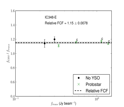
(a)

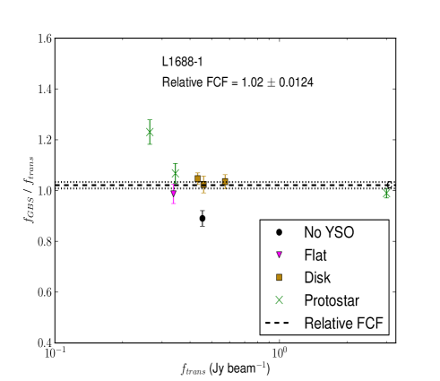
(c)

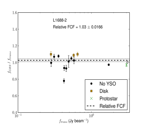
(d)

Figure 1: The mean GBS peak brightness divided by the mean Transient Survey peak brightness for all sources brighter than 200 mJy beam^-1 with radii less than $10\arcsec$ in the Perseus (top) and Ophiuchus (bottom) Molecular Cloud fields. The ratios are plotted against their mean peak brightnesses as measured across the Transient Survey. Points labeled with a “c” are chosen to be calibrators (Family members) in both the GBS and Transient Survey data independently. Each point is coloured according to its association with YSOs (see text and legend). The error bars represent the combination of the uncertainty in the rescaled GBS peak brightness measurements and the uncertainty in the Transient Survey peak brightness measurements. The dashed line represents the derived relative flux calibration factor between the GBS data and the Transient Survey data (the number by which to divide to bring the GBS data into relative calibration with the Transient Survey data). The dotted lines represent the FCF uncertainty.

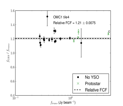
(a)

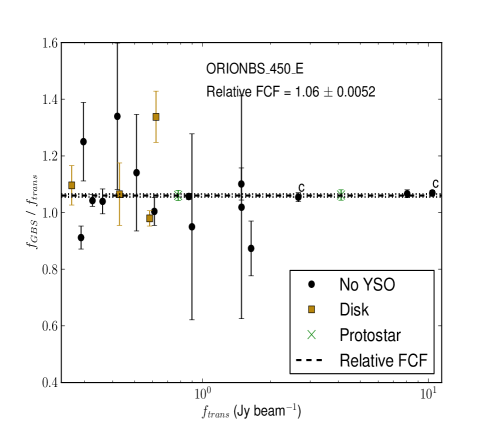
(c)

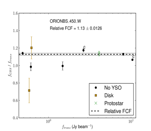
(d)

Figure 2: Same as Figure 2 for the Orion A and B Molecular Cloud fields.

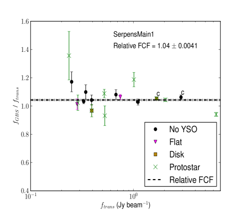
(a)

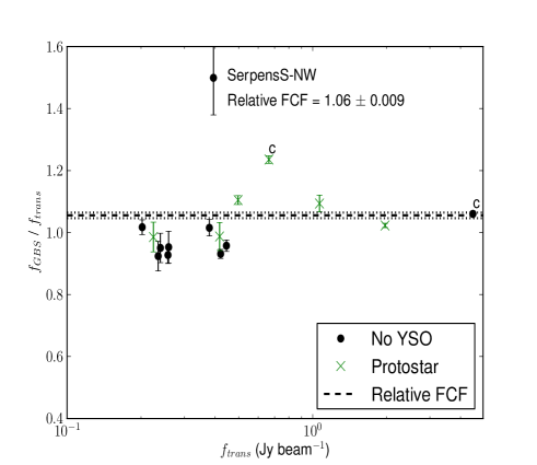
(c)

Figure 3: Same as Figure 2 for the Serpens Molecular Cloud fields.

In order to bring the GBS data and the Transient Survey data into relative flux calibration with one another, we first identify sources common to both surveys. The sources we select have peak brightnesses larger than $200\mathrm{\>mJy\>beam}^{-1}$ and effective radii less than $10\arcsec$. For each source, we measure the average peak brightness ($f_{\mathrm{GBS}}$ and $f_{\mathrm{trans}}$) and derive the associated uncertainties ($\sigma_{f_{\mathrm{GBS}}}$ and $\sigma_{f_{\mathrm{trans}}}$) by calculating the measured standard deviation across all observations within each survey individually and dividing the result by the square root of the number of observations that were included in the calculation (see Table 2).

We calculate a calibration factor using the measured source brightnesses by dividing the $f_{\mathrm{GBS}}$ values by their corresponding $f_{\mathrm{trans}}$ values. For the $i^{th}$ source, we label this ratio $R_{i}$ and we propagate the uncertainties, $\sigma_{R,i}$, in order to calculate the weighted mean, $\bar{R}$,

$$\bar{R}=\frac{\sum_{i=1}^{n}R_{i}w_{i}}{\Sigma_{i=1}^{n}w_{i}},$$ (1)

where $n$ is the number of sources and the weights are the inverse square of the propagated uncertainties,

$$w_{i}=\sigma_{R,i}^{-2}.$$ (2)

The uncertainty in the weighted mean, $\sigma_{\bar{R}}$, is given by

$$\sigma_{\bar{R}}=\sqrt{\frac{1}{\Sigma_{i=1}^{n}w_{i}}}.$$ (3)

Next, we calculate the difference, $\delta$, between each peak brightness ratio and the weighted mean by subtracting the latter from the former and dividing by the uncertainty associated with that source added in quadrature to the uncertainty in the weighted mean,

$$\sigma_{\mathrm{tot},i}=\sqrt{\sigma_{R,i}^{2}+\sigma_{\bar{R}}^{2}}$$ (4)

$$\delta_{i}=\frac{R_{i}-\bar{R}}{\sigma_{\mathrm{tot},i}}.$$ (5)

We consider all sources with $\lvert\delta\rvert>3$ to be deviant outliers that might skew the weighted mean. Therefore, we remove these sources from the calculation and recompute the weighted mean. This refined weighted mean (that excludes outliers) represents the initial approximation of the relative flux calibration factor between overlapping average GBS and Transient Survey images.

To explore how the peak brightness uncertainties in each data set ($\sigma_{f_{\mathrm{GBS}}}$ and $\sigma_{f_{\mathrm{trans}}}$) affect the refined weighted mean, we use a Monte Carlo analysis. We fix $\sigma_{f_{\mathrm{GBS}}}$ and $\sigma_{f_{\mathrm{trans}}}$ for each source and randomly draw new peak brightness measurements from normal distributions with mean values equal to $f_{\mathrm{GBS}}$ and $f_{\mathrm{trans}}$ and standard deviations equal to $\sigma_{f_{{\mathrm{GBS}}}}$ and $\sigma_{f_{\mathrm{trans}}}$. In this way, we calculate a new peak brightness ratio for each source, $R_{i}$, that is within the derived measurement uncertainties. Then, we calculate a new weighted mean (Equation 1) based on these values, discard outliers in the same manner as before, and compute a refined weighted mean. We repeat this process 10,000 times.

Of these 10,000 refined weighted mean values, we adopt the average as the relative flux calibration factor, or, relative FCF. This is the number by which we divide the GBS image to bring it into relative calibration with the Transient Survey image. The standard deviation in refined weighted mean values is the uncertainty in the relative FCF, $\sigma_{\mathrm{FCF}}$.

We plot the results in Figures 2 through 2. The colours represent a source’s association with known YSOs. In these figures, to be associated with a protostar, flat spectrum source, protostellar candidate, or disk, the peak position of the source must be within 10$\arcsec$ of the YSO location (to match the radius of the largest compact source we consider). Points labelled with a “c” are Family Members in both the GBS and Transient Surveys, i.e. they appear to have stable peak brightnesses in each dataset independently but not necessarily when compared over several year timescales. The FCF values are indicated by the dashed lines and $\sigma_{\mathrm{FCF}}$ is indicated by the dotted lines. As the noise is relatively constant across a map and large scale modes have been mostly removed in the data reduction procedure, we expect the relative FCF value to remain constant across the full field of any single image.

The GBS images were all originally calibrated at a level that is slightly brighter than their respective Transient Survey images obtained prior to March 1^st, 2017. This is the result of several factors that affect the nominal flux calibration performed at the JCMT, before we apply the relative flux calibration presented above. For instance, the nominal flux calibration values are based on data obtained between 2011 and 2012 (Dempsey et al., 2013), the water vapour monitor was replaced in 2015, and SCUBA-2 had a filter upgrade in late 2016. The combination of these factors have led to differences in the original calibration of the data obtained in the GBS and the Transient Survey eras. These effects are corrected for by our relative flux calibration.

4 Results

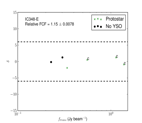
(a)

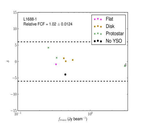
(c)

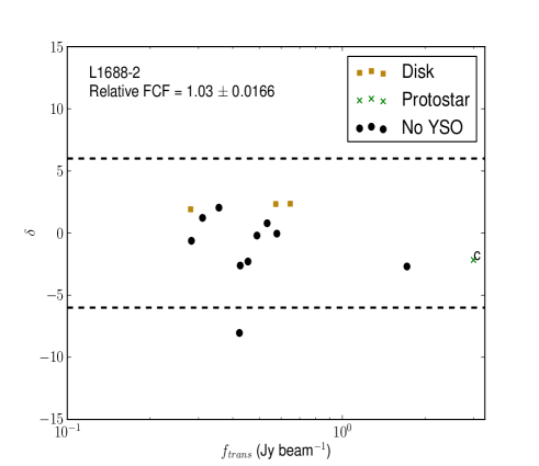
(d)

Figure 4: The deviation from the FCF for all sources brighter than 200 mJy beam^-1 with radii $<10\arcsec$ in the Perseus (top) and Ophiuchus (bottom) Molecular Cloud fields. The ratios are plotted against their mean peak brightness as measured across the Transient Survey. Points labeled with a “c” are chosen to be calibrators (Family members) in both the GBS and Transient Survey data independently. Each point is coloured according to its association with YSOs (see text and legend). Dashed lines are drawn at $\pm 4$ to highlight sources defined to be significant outliers.

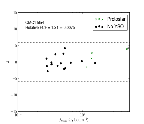
(a)

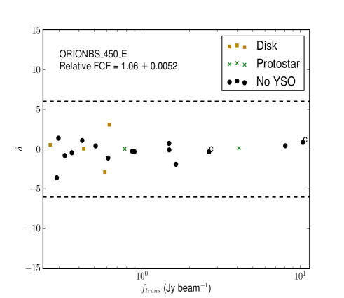
(c)

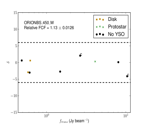
(d)

Figure 5: Same as Figure 2 for the Orion A and B Molecular Cloud fields.

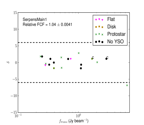
(a)

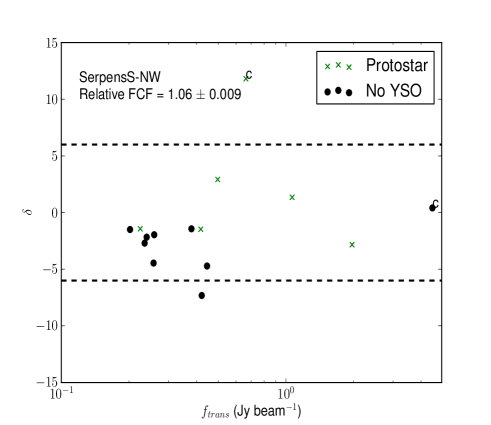
(c)

Figure 6: Same as Figure 2 for the Serpens Molecular Cloud fields.

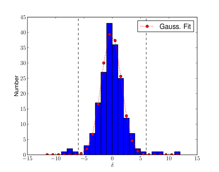
Figure 7: The distribution of $\delta$ values for all sources. The red points represent a Gaussian fit to the histogram. The vertical dashed lines indicate the threshold for a significant detection of a variable candidate.

Table 2: Summary of the variable candidate source properties.

GBS Field	ID	Other Name	R.A. (J2000)	Dec (J2000)	$f_{\mathrm{trans}}$	$\frac{\sigma_{f_{\mathrm{trans}}}}{f_{\mathrm{trans}}}$	$f_{\mathrm{GBS}}$b	$\frac{\sigma_{f_{\mathrm{GBS}}}}{f_{\mathrm{GBS}}}$c	$\lvert\delta\rvert$	$\frac{\dot{f}}{f_{\mathrm{trans}}}$ (% yr-1)	$\sigma_{\dot{f}/f}$	Category
NGC1333-N	PER-1	IRAS4A	3:29:10.42	31:13:30.63	8.83	1.0	8.10	0.4	7.66	2.09	0.28	S
NGC1333-N	PER-10	Bolo 40	3:28:59.86	31:21:33.09	0.60	1.0	0.67	0.7	7.99	-3.03	0.36	S
NGC1333-N	PER-34	[LAL96] 213	3:29:07.66	31:21:54.05	0.28	2.8	0.38	1.2	8.31	-8.64	0.87	S
SerpensMain1	SER-1	[KOB2004] 258b	18:29:49.80	1:15:19.33	6.38	1.5	5.76	0.4	6.85	2.37	0.39	S
SerpensS-NW	SER-10	IRAS 18270-0153	18:29:37.99	-1:51:04.66	0.66	0.8	0.78	0.6	11.81	-4.05	0.35	S
L1688-2	OPH-14	–	16:26:24.95	-24:24:23.92	0.42	1.9	0.32	2.7	8.04	6.10	0.78	E
SerpensS-NW	SER-21	SerpS-MM15	18:30:02.69	-2:01:09.33	0.42	0.9	0.37	1.3	7.32	2.82	0.38	E
OMC1 tile4	ORA-36	HOPS 383	5:35:29.67	-4:59:37.25	0.53	0.9	0.58	1.6	4.17	-2.66	0.64	Pos.

In Section 3.2, above, we described how we bring the mean GBS data and the mean Transient Survey data into relative flux calibration with one another by using the bright, compact sources in each overlapping field. Once the relative FCF has been computed, we repeat our calculation to search for significant outliers by replacing the individually calculated weighted mean of the source peak ratios, $\bar{R}$, with the mean FCF and $\sigma_{\bar{R}}$ with $\sigma_{\mathrm{FCF}}$ in Equation 5. Here, we define the significance of outliers based on the distribution of these newly calculated $\delta$ values.

Figures 2 to 2 show the $\delta$ value of every source. In Figure 7, we show the distribution of $\delta$ values for all sources fit with a Gaussian curve. The fitted Gaussian has a standard deviation of $\sigma_{GaussFit}=1.76$. The measured $\delta$ values significantly deviate from the fitted Gaussian profile beyond a threshold of $\delta=\pm 6$. Therefore, we define sources that have $\lvert\delta\rvert>6$ as noteworthy outliers. The probability of detecting a source with $\lvert\delta\rvert>6$ from the Gaussian distribution of values is 0.06%. Over all 11 GBS fields that overlap with the Transient Survey data, however, we find that 7 out of 175 independent sources brighter than 200 mJy beam^-1 with radii <10″ exceed this threshold. Thus, 96% of the identified sources show no sign of variation between the average GBS data and the average Transient data to our sensitivity, while the remaining 4% are considered variable candidates and form the basis of all further investigation. We summarise the properties of the variable candidates in Table 2.

In order to discern the quality of each of the variable candidates, we construct difference maps, subtracting the GBS co-add from the Transient co-add for each region, and perform a visual analysis on each map to note sources with extended features in confused regions as well as larger-scale differences between the maps which can complicate our measurements (see Figures 2 and 19 in Appendix A).

Table 3: Associations between variable candidate and YSOs.

GBS Field	ID	Other Name	Nproto	Distproto	Category
NGC1333-N	PER-1	IRAS4A	2	2.64	S
NGC1333-N	PER-10	Bolo 40	0	–	S
NGC1333-N	PER-34	[LAL96] 213	1	2.56	S
SerpensMain1	SER-1	[KOB2004] 258b	1	3.16	S
SerpensS-NW	SER-10	IRAS 18270-0153	1	6.22	S
L1688-2	OPH-14	–	0	11.31	E
SerpensS-NW	SER-21	SerpS-MM15	0	–	E
OMC1 tile4	ORA-36	HOPS 383	0	13.49	Pos.

Table 4: Associations between 850 $\mu$m emission sources and YSOs.

	# 850 $\mu$m Sources	# With Proto (10$\arcsec$)	# With Disk (10$\arcsec$)	# With no known YSO
Total	175	54	13	108
Strong Var. Can.	5 (3%)	4 (7%)	0 (0%)	1 (1%)
All Var. Can.	7 (4%)	4 (7%)	0 (0%)	3 (3%)

While investigating the difference maps, we searched for any indication of compact sources that were present only in the GBS data and not in the Transient Survey data (or vice versa) in case an object had varied such that it fell below the detection threshold (200 mJy beam^-1) in one dataset but not in the other. No significant objects of this type were identified.

Through our visual inspection of each source in their respective difference maps, we define 2 categories of variable candidate:

• Strong Candidates (S): The source exceeds the significance threshold ($\lvert\delta\rvert>6$), has an average Transient Survey peak brightness measurement of $f_{\mathrm{trans}}>200\mathrm{\>mJy\>beam}^{-1}$, and has a radius less than 10$\arcsec$. These sources have an obvious indication of significant compact structure at the location of the source in the difference map.

• Extended Candidates (E): The source exceeds the significance threshold ($\lvert\delta\rvert>6$), has an average Transient Survey peak brightness measurement of $f_{\mathrm{trans}}>200\mathrm{\>mJy\>beam}^{-1}$, and a radius less than 10$\arcsec$. There is little indication of compact structure present at the location of the source in the difference map; surrounding extended structures complicate the measurements.

We find 5 Strong sources and 2 Extended sources. Extended variable candidates display very little evidence of real compact emission changing brightness between the GBS and Transient Survey datasets. It is likely that we are underestimating the uncertainty for these objects due to the uncertainty in the background subtraction computed by the Gaussclumps algorithm in confused areas. Both of these remain interesting sources, though they are less robust candidates for variability than those classified as Strong. The Extended source OPH-14 traces part of the larger scale structure around the prototypical Class 0 source VLA 1623 (Andre et al., 1993), though we see no significant evidence that the deeply embedded protostar itself is undergoing a significant brightness change at 850 $\mu$m. In addition to the Strong and Extended candidates, one Possible candidate (HOPS 383; Safron et al. 2015) is also identified in Tables 2 and 3 and is discussed further in Section 5.1.

In general, we expect the presence of a disk to influence the accretion rate of material onto the central protostar. Of the 5 Strong variable candidates, 4 are associated with a known protostar (and likely, therefore, a young circumstellar disk) and none are associated with a known evolved disk object (see N_proto in Table 3; see also Table 4). To be associated with a protostar or a disk, the peak position of the source must be within 10$\arcsec$ of the YSO location. Recall that the presence of a dusty envelope increases the likelihood of detecting variability at submillimetre wavelengths due to the reprocessing of the light emitted by a burst event. Generally, the envelope is faint or non-existant for known, more evolved disk candidates seen at infrared wavelengths.

In total, out of the 175 independent sources identified across all 8 Transient Survey fields and their 11 associated GBS fields, there are 54 protostars and 13 disk objects within 10$\arcsec$ of source peaks. Therefore, to the sensitivity achieved across these surveys, approximately 7% of known protostars associated with an 850 $\mu$m emission source to be potentially varying. Only 3% of the sources not known to be associated with a YSO show signs of variability. One of the Strong variable candidates, IRAS4A (PER-1), has two protostars associated with its peak. Another, SER-1, displays an elongated structure that may indicate multiple embedded sources or some outflow activity. Excluding the Extended sources, which are less robust detections, only one source without a known protostar or disk shows signs of variability. We do not expect starless cores to be variable. Therefore, the Strong variable candidate without a known embedded YSO, Bolo 40 (Enoch et al., 2006), is a good target for follow-up studies to identify signatures of very faint, deeply embedded protostars that have yet to be detected.

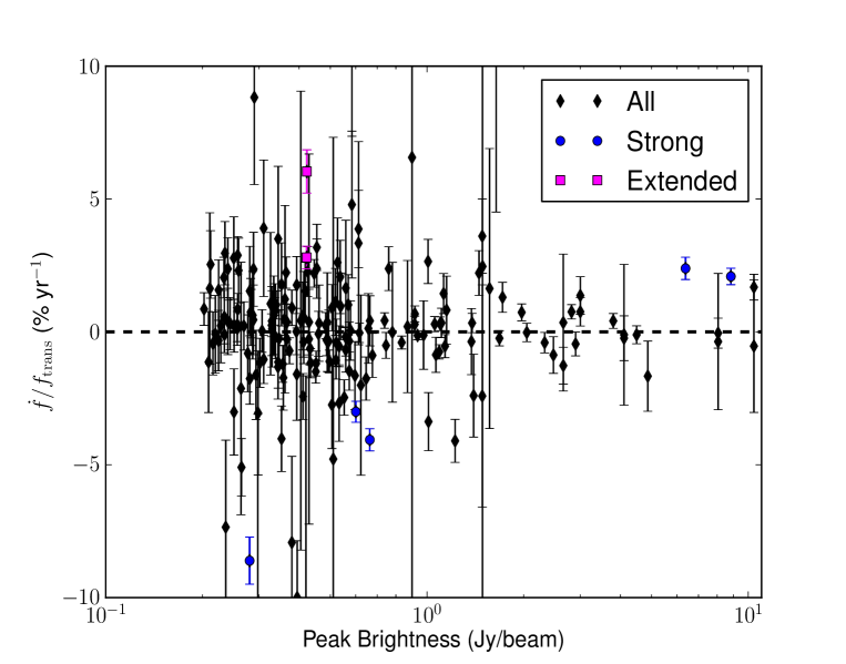
Figure 8: The change in peak brightness divided by the difference between the average GBS and Transient Survey observation dates, normalised to the average Transient Survey peak brightness (($\dot{f}/f_{\mathrm{trans}}$), Equation 6). Strong variable candidates are indicated by blue circles. Extended variable candidates are indicated by magenta squares. All other sources are indicated by black diamonds. Variable candidates are intermixed with non-variable sources as the detection sensitivity varies from field to field (see Table 5).

The GBS data and the Transient Survey data were obtained 2-4 years apart, depending on the field (see Table 2), which allows us to characterise the apparent, significant submillimetre brightness changes in terms of a fractional change per year (averaged over both datasets) assuming a linear change throughout the GBS/Transient Survey time lag,

$$\frac{\dot{f}}{f_{\mathrm{trans}}}=\frac{f_{\mathrm{trans}}-f_{\mathrm{GBS}}}{f_{\mathrm{trans}}}\times\left(\frac{1}{\bar{t}_{\mathrm{trans}}-\bar{t}_{\mathrm{GBS}}}\right),$$ (6)

where $\bar{t}_{\mathrm{GBS}}$ is the mean GBS observation date for that field and $\bar{t}_{\mathrm{trans}}$ is the mean Transient Survey observation date for that field (the parenthetical term in the denominator is the same as $\Delta t$ in Table 2). We choose to normalise the result to the mean Transient Survey observation to express the brightness change as a percentage of the (near) current source peak brightness. The associated error, $\sigma_{\dot{f}/f}$, is the combination of the Transient Survey average peak brightness error (see Section 3.2 and Table 2), the GBS peak brightness error, and the error in the weighted mean.

Table 5: Current $\dot{f}/f_{\mathrm{trans}}$ sensitivity limits.

GBS Field	$\Delta f$ Sensitivity Limit (%yr-1)	Typical $\Delta f$ Sensitivity (%yr-1)
IC348-E	2.2	2.9
L1688-1	3.3	5.0
L1688-2	2.9	4.8
NGC1333-N	1.4	3.6
OMC1 tile4	2.0	4.3
OrionBN_450_S	3.7	7.4
OrionBS_450_E	3.8	17.7
OrionBS_450_W	2.4	4.7
SerpensMain1	1.1	5.0
SerpensS-NE	1.0	4.6
SerpensS-NW	1.5	3.8

We plot $\dot{f}/f_{\mathrm{trans}}$ as a function of the Transient Survey average peak brightness in Figure 8, coloured according to category. A typical, Strong variable candidate has an average brightness change per year of $\lvert 4.0\rvert\%\mathrm{\>yr}^{-1}$ with a standard deviation of $2.7\%\mathrm{\>yr}^{-1}$. The Extended variable candidates are grouped in a similar area of parameter space. This grouping is primarily the result of poor background flux subtraction performed by the Gaussclumps algorithm in these more confused regions. This strengthens the notion that the uncertainties in these measurements are likely underestimated. Every calibrated GBS field includes a distribution of sources that appear slightly brighter and slightly fainter than their Transient Survey counterparts. The brightest Strong candidates all display a positive $\dot{f}/f_{\mathrm{trans}}$, while the fainter Strong candidates all show significant brightness decreases between the GBS and Transient Survey eras. This may indicate an intrinsic difference in the underlying accretion process for different types of protostars. This trend, however, is only based on small number statistics.

Three factors contribute to the sensitivity of $\lvert\dot{f}/f_{\mathrm{trans}}\rvert$: the uncertainties in the GBS and Transient Survey peak brightness measurements, the uncertainty in the calibration, and the time lag between the two data sets for each field (see $\Delta t$ in Table 2). In Table 5, we present both the sensitivity limit and the typical sensitivity in $\lvert\dot{f}/f_{\mathrm{trans}}\rvert$ for each field. To calculate the sensitivity limit for each field, we set Equation 5 (replacing $\bar{R}$ with the mean FCF and $\sigma_{R}$ with $\sigma_{\mathrm{FCF}}$) equal to 6 (the threshold at which we define a source to be a variable candidate) and solve for the GBS peak brightness in terms of the Transient Survey peak brightness. Then, we substitute the result into Equation 6 for each source and find the minimum allowed $\lvert\dot{f}/f_{\mathrm{trans}}\rvert$ for a variable candidate in each field. For the typical $\lvert\dot{f}/f_{\mathrm{trans}}\rvert$ sensitivity, we report the median $\lvert\dot{f}/f_{\mathrm{trans}}\rvert$ value calculated in this fashion. As the Transient Survey continues and we are able to observe longer time separations, our sensitivity will improve.

5 Discussion

The relative flux calibration agreement between GBS fields associated with the same Transient Survey field is robust. There are 13 sources in total that overlap two GBS fields and a Transient Survey field. There are no cases where a source is considered to be a variable candidate in one GBS field and not the other. In total, we find 7 sources with significantly discrepant GBS to Transient Survey peak brightness ratios, indicating they are candidates for variability. These sources are distributed around $\dot{f}/f_{\mathrm{trans}}=0\%\mathrm{\>yr}^{-1}$ (Figure 8). Though we do not necessarily expect linear changes over 2-4 year timescales, assuming linearity, the average $\lvert\dot{f}/f_{\mathrm{trans}}\rvert$ of the Strong variable candidates over several year timescales using co-added, well calibrated maps is $\lvert 4.0\rvert\%\mathrm{\>yr}^{-1}$ with a standard deviation of $2.7\%\mathrm{\>yr}^{-1}$ (see Table 2 and Figure 8). We are not sensitive to short timescale, small fluctuations that may average out the signal over time (see Section 5.2 for a further example of the limitations of time averaging), so we expect there to be more variable candidates in these fields that can be identified at higher time resolutions and sensitivities. An analysis of variability within the Transient Survey data alone is addressed by Johnstone et al., (in preparation).

The observed difference in the submillimetre flux of an embedded protostar undergoing a change in accretion rate is determined by the heating or cooling of the dusty envelope. As long as the dust temperature remains above $\sim$25 K, the sub-mm response will be approximately linear to this change in temperature. When the dust temperature is lower, the submillimetre response becomes much stronger. In equilibrium, the dust temperature, $T_{\mathrm{dust}}$, in most of the envelope is expected to vary with accretion luminosity, $L_{\mathrm{acc}}$, as $T_{\mathrm{dust}}\propto L_{\mathrm{acc}}^{1/4}$ (Johnstone et al., 2013). As Johnstone et al. (2013) note, however, this relationship will break down in the very outer envelope where significant heating comes from the external radiation field and therefore the temperature of the dust remains relatively fixed.

For small fractional changes in temperature, the accretion luminosity is approximated by

$$\frac{\Delta L_{\mathrm{p}}}{L_{\mathrm{p}}}\propto 4\times\frac{\Delta T_{\mathrm{dust}}}{T}.$$ (7)

Assuming the submillimetre response is roughly proportional to the dust temperature which itself is determined primarily by the accretion luminosity, a 4% change in the observed submillimetre flux corresponds to a $\sim$16% change in the accretion luminosity (accretion rate) of the central protostar. If the envelope temperature drops below $\sim$25 K, then the submillimetre response will be closer to one-to-one (i.e. a 4% change in the observed submillimetre flux corresponds to $\sim$4% change in accretion luminosity). Much work is still required to fully understand the relationship between the observed submillimetre flux and the accretion luminosity (see, for example, Johnstone et al. 2013).

We find 7% of the known protostars in our observed fields display a typical $16\%$ accretion variability over $\sim$3 years (using Equation 7). In Figure 3 of Herczeg et al. (2017), the authors summarise expectation values of accretion variability over specific timescales, taking into consideration a model in which the variability is driven by large-scale gravitational instabilities in the disk (Vorobyov & Basu, 2010) and a model in which smaller-scale magneto-rotational instabilities are included Bae et al. (2014). The models of Vorobyov & Basu (2010) predict that $\sim$7% of protostars will undergo a 7%-8% change in accretion luminosity over 3 years of observations. Bae et al. (2014), however, predict that $\sim 7\%$ of protostars will undergo a 40% change in accretion luminosity over this same timeframe. Under the simple assumption that submillimetre brightness varies linearly as dust temperature, Equation 7 predicts our results to lie between the two models. We note, however, that this result is tempered by uncertainties in the relationship between changes in the submillimetre flux due to the protostellar luminosity, the reliability expected from the models of protostellar episodic accretion over few year timsescales (as a detailed investigation relies on accurately tracing the physics of the inner disk), and the sensitivity of our source detection methods.

Future surveys studying accretion variability onto deeply embedded protostars would benefit from working in the far infrared, near the peak of the protostellar envelope spectral energy distribution in order to have a more linear relationship between observed brightness changes and the underlying accretion luminosity variation (see Johnstone et al., 2013). These surveys are likely to be undertaken by space observatories such as the Space Infrared Telescope for Cosmology and Astrophysics (SPICA; Roelfsema et al., submitted) or the Origins Space Telescope (OST; Meixner et al. 2016) which will further benefit from the stability of space-based observations, provided that the calibration and dynamic range of the instruments is excellent. As these missions are still a decade or more away, an obvious first undertaking will be to use Herschel Space Observatory observations of nearby star-forming regions as a previous epoch, yielding a multi-decade delta in time. As this paper shows, however, there are significant challenges in collating two disparate data sets and thus care will need to taken in order to reach relative uncertainties at the $1\%-2\%$ level.

5.1 Previously Known Signatures of Variability

Nearly all of the submillimetre emission sources in Table 2 are detected in previous surveys (see, for example, Johnstone et al., 2000, 2001; Skrutskie et al., 2006; Kirk et al., 2006; Di Francesco et al., 2008), and many have been associated with outflows. Two Strong sources have previously-known indicators of variability from outflow knots or inferences from spectroscopic diagnostics: IRAS4A (PER-1) and IRAS 18270-0153 (SER-10).

In the case of IRAS4A, the evidence is in the form of outflowing jets with compact knots (Choi, 2001), a phenomenon that has been characterised around protostellar and Herbig-Haro objects for many years (see, for examples, Reipurth, 1989; Cernicharo & Reipurth, 1996; Reipurth et al., 2004, and references therein). These jets may be caused by episodic outbursts (Choi, 2001) that increase the density of the ejected material for a short period of time, leaving some indication of the history of activity around the source. Other evidence, however, points to jet precession as the source of the knots (Choi et al., 2006; Santangelo et al., 2015).

IRAS 18270-0153 (Connelley et al., 2007) has been classified as an “FU Orionis-like” object, owing to its deep CO and water vapour absorption bands and lack of clearly defined photospheric absorption lines (Greene & Lada, 1996; Connelley & Greene, 2010). These features indicate the presence of a very hot, optically thick inner disk, which is a signpost for an ongoing FUor accretion outburst (Zhu et al., 2007). In addition, this protostar has a notable bipolar outflow in H₂ (Zhang et al., 2015). We observe a decrease in brightness at the rate of 4.3% yr^-1, assuming a linear change.

In addition to these Strong candidates, we highlight one further source of interest, ORA-36 (HOPS 383; Safron et al. 2015), which we list as a Possible variable candidate in Tables 2 and 3. HOPS 383 is a source that contains the youngest known Class 0 protostar that has shown evidence of an outburst in both infrared and submillimetre data (Safron et al., 2015). Mid- and far-infrared photometric data indicate that the source underwent a strong outburst between 2004 and 2012. By comparing 450 $\mu$m Submillimetre Common-User Bolometre Array (SCUBA) data from 1998 to 350 $\mu$m Submillimetre APEX Bolometer Camera (SABOCA) data in 2011, Safron et al. (2015) found that the source had doubled in brightness in the submillimetre. We expect that an accretion outburst would be much brighter in the infrared (Johnstone et al., 2013). Here, we see a clear indication of a compact emission source closely associated with HOPS 383. We do not consider it a robust variable candidate as its $\delta$ value is less than 6 ($\delta=4.17$; see Table 2), though it appears to be undergoing a brightness decrease between the GBS and Transient Survey data at the level of $-2.66\pm 0.64\%\>\mathrm{yr}^{-1}$. Fischer & Hillenbrand 2017 have also noted a recent brightness decrease in the $H$ and $K$-bands for this source. The extracted 2D Gaussian source traces an extended structure in which the compact feature is embedded (see Figure 2), causing the peak of the identified source to artificially shift further from the protostar it contains.

In addition to the variables, some non-varying sources are also of interest. Our observations coincide with 2 long-term radio (cm wavelength) variable sources in IC 348 (VLA 2 and VLA 3; Forbrich et al. 2011), but neither are significantly variable at 850 $\mu$m. VLA 2 was found to decrease in brightness from 0.09 mJy in 2001 (Avila et al., 2001) to 0.04 mJy in 2008, In this work, we have found no significant brightness change between the GBS and Transient Survey observations ($\delta=0.81$) for the associated 850 $\mu$m emission source. Similarly, we find no 850 $\mu$m emission source to coincide with VLA 3, which increased in radio brightness from 0.41 mJy in 2001 Avila et al. (2001) to 0.542 mJy in 2008, It is important to recognise that radio and submillimetre variability arise from different phenomena. In the former case, magnetic flares and synchrotron radiation dominate while in the latter case we are tracing accretion events.

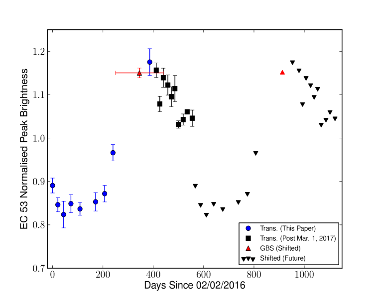
(b)

Figure 9: The 850 $\mu$m light curve of EC 53 (see also, Yoo et al. 2017). Top: The red (upward) triangle represents the average, calibrated GBS data, the blue circles represent data analysed in this paper, and the black squares represent data that has been collected between March 1^st, 2017 and July 5^th, 2017. Bottom: The black (downward) triangles represent all obtained Transient Survey data shifted one period (567 days) into the future. The GBS data presented in this Figure has been shifted three and then four increments of 567 days until it matched the current and next periodic cycles. The error bars in the GBS dates suggest a reasonable range of values that agree with the rise in the light curve.

5.2 The Period of the Submillimetre Variable EC 53

One prominent source in the Serpens Main Transient Survey field, EC 53 (Eiroa & Casali, 1992), is identified as a sub-mm variable in a companion paper (Yoo et al., 2017) and has previously been identified as a periodic variable in near-IR ($K$-band) photometry (Hodapp et al., 2012). The periodicity is thought to be driven by accretion instabilities triggered by a nearby companion (Hodapp et al., 2012). We do not detect it as a variable candidate in this paper ($\delta=2.83$) because EC 53’s periodicity is timed such that the difference between the GBS measurement and the average Transient measurement is only moderate. In addition, the uncertainty (standard deviation) in EC 53’s time averaged brightness across the Transient Survey data is high, because the brightness change over one period is significant (see Johnstone et al., in prep. for an analysis performed at a higher time resolution). To make this more clear, the source’s 850 $\mu$m light curve presented in Figure 2 (see also, Yoo et al. 2017). In the top panel, the GBS and Transient peak brightness data are plotted against the dates of observation. The red (upward) triangle represents the average, calibrated GBS data, the blue circles represent Transient Survey data included in the investigation presented in this paper (obtained between February 2^nd, 2016 and February 22^nd, 2017), and the black squares represent Transient Survey data obtained between March 1^st, 2017 and July 5^th, 2017. The Transient Survey error bars represent the standard deviation of the normalised peak brightnesses across the Family of calibrator sources for each epoch (whereas the uncertainty of the GBS data point includes all 4 GBS observations taken over two nights, see Table 2).

In the bottom panel, we shift the calibrated GBS data from its original observation date until it reasonably aligns with the Transient Survey observation dates. We find that a shift of 1700 days from the original observation date agrees well with the rise of the peak brightness (red, upward triangle) with a range of acceptable values from 1605 days to 1795 days (horizontal, red errorbars). A shift of 1700$\pm$95 days corresponds to 3 full periods of 567 $\pm$ 32 days at 850 $\mu$m. To this accuracy, we independently confirm the 850 $\mu$m periodicity is consistent with the 543 day $K$-band periodicity (Hodapp et al., 2012). In order to show the periodic nature of EC 53, we assume the cycle is continuously repeating and we display all of the obtained Transient Survey observations shifted by 567 days (black, downward triangles), once again including the average GBS data in this future cycle.

6 Summary and Conclusions

In this paper, we investigate signatures of 850 $\mu$m submillimetre variability by comparing archival GBS fields, observed between 2012 and 2014, to JCMT Transient Survey fields, observed between December 2015 and March 1^st 2017. We follow the data reduction and calibration procedures presented in Mairs et al. (2017) to self-consistently align and calibrate each set of observations from the two surveys individually before bringing the co-added GBS images into relative flux calibration with the co-added Transient Survey images (see Section 3 and Figures 2 through 2). Using the source extraction algorithm Gaussclumps (Stutzki & Guesten, 1990), we identify 175 independent bright (>200 mJy beam^-1), compact (effective radius <10$\arcsec$) compact emission objects that were well fit with Gaussian profiles, correlate them with known protostars (Class 0+I, Flat spectrum sources; see Section 2.3) and disks (Class II sources), and identify objects that are significant outliers in their GBS to Transient Survey average peak brightness ratio with respect to the other sources in the field (see Figures 2 through 2, Figure 7 and Equation 5). Based on a visual inspection for compact structure present around the area of each outlying source in calibrated difference maps (the Transient Survey co-add subtracted from the GBS co-add), we define two categories for the quality of each variable candidate.

Our main results are summarised as follows:

1. We have developed methods to robustly analyze repeated observations of an area of the sky for signatures of submillimeter variability. We identify 11 archival GBS fields that can be self-consistently flux calibrated and have significant overlap with the 8 Transient Survey fields (see Appendix A).

2. Out of 175 independent compact, 850 $\mu$m emission sources, we find a total of 7 variable candidates, 4 of which are associated with known protostars.

3. We classify 5 of the variable candidates as Strong and 2 as Extended (see Section 4), and we highlight one additional source, HOPS 383, as a Possible detection of variability. Two Strong sources (IRAS4A, IRAS 18270-0153) along with HOPS 383 have previously noted signatures of variability. There is one Strong variable candidate without a known protostellar or disk association (Bolo 40/PER-10). This is a good target for follow-up studies to identify signatures of very faint, deeply embedded protostars (see Table 2).

4. The average flux change for the strong variable candidates is $\lvert 4.0\rvert\%\mathrm{\>yr}^{-1}$ with a standard deviation of $2.7\%\mathrm{\>yr}^{-1}$ over 2-4 year timescales. Assuming the heating of the envelope is responsible for the changing luminosity, this corresponds to a change in accretion rate of $\sim 16\%$ (see Section 5). The observed changes in flux for all sources are distributed around $0\%\mathrm{\>yr}^{-1}$.

5. Using the archival GBS data, we strengthen the detection of the submillimetre variable source EC 53 by adding a critical data point to its periodic light curve and determine its 850 $\mu$m period to be 567 $\pm$ 32 days. This value is consistent with the 543 day period perviously reported in the $K$-band (see Figure 2, Yoo et al. 2017, and Hodapp et al. 2012).

Throughout this work, we have developed methods to robustly analyse repeated observations of an area of the sky for signatures of submillimetre variability. The JCMT Transient Survey will continue through at least January, 2019 and as more data are collected we will have the opportunity to continue this investigation to fainter sources and smaller levels of variability over longer timescales. Future directions include periodically co-adding sets of Transient Survey observations to construct very precise light curves (sacrificing temporal resolution for higher sensitivity), improving the flux calibration procedures such that more archival data can be included, comparing these observations with the simultaneous 450 $\mu$m datasets once the latter can be robustly reduced and calibrated, and applying these observational constraints to current simulations of variable protostellar accretion.

Acknowledgements

Steve Mairs was partially supported by the Natural Sciences and Engineering Research Council (NSERC) of Canada graduate scholarship program. Doug Johnstone is supported by the National Research Council of Canada and by an NSERC Discovery Grant. Gregory Herczeg is supported by general grant 11473005 awarded by the National Science Foundation of China. Andy Pon received partial salary support from a Canadian Institute for Theoretical Astrophysics ( CITA) National Fellowship. Miju Kang was supported by Basic Science Research Program through the National Research Foundation of Korea (NRF) funded by the Ministry of Science, ICT & Future Planning (No. NRF-2015R1C1A1A01052160).

The authors wish to recognise and acknowledge the very significant cultural role and reverence that the summit of Maunakea has always had within the indigenous Hawaiian community. We are most fortunate to have the opportunity to conduct observations from this mountain. The James Clerk Maxwell Telescope is operated by the East Asian Observatory on behalf of The National Astronomical Observatory of Japan, Academia Sinica Institute of Astronomy and Astrophysics, the Korea Astronomy and Space Science Institute, the National Astronomical Observatories of China and the Chinese Academy of Sciences (Grant No. XDB09000000), with additional funding support from the Science and Technology Facilities Council of the United Kingdom and participating universities in the United Kingdom and Canada. The James Clerk Maxwell Telescope has historically been operated by the Joint Astronomy Centre on behalf of the Science and Technology Facilities Council of the United Kingdom, the National Research Council of Canada and the Netherlands Organisation for Scientific Research. Additional funds for the construction of SCUBA-2 were provided by the Canada Foundation for Innovation. The identification number for the JCMT Transient Survey data used in this paper is M16AL001. The identification numbers for the archival Gould Belt Survey data used in this paper are: MJLSG31, MJLSG32, MJLSG33, MJLSG38, and MJLSG41. The authors thank the JCMT staff for their support of the data collection and reduction efforts. This research has made use of NASA’s Astrophysics Data System and the facilities of the Canadian Astronomy Data Centre operated by the National Research Council of Canada with the support of the Canadian Space Agency. The authors would especially like to thank Chang Won Lee and Harriet Parsons for their useful insights and suggestions along with the extended JCMT Transient Team for their support. This research used the services of the Canadian Advanced Network for Astronomy Research (CANFAR), which in turn is supported by CANARIE, Compute Canada, University of Victoria, the National Research Council of Canada, and the Canadian Space Agency. This research made use of APLpy, an open-source plotting package for Python hosted at http://aplpy.github.com, and matplotlib, a 2D plotting library for Python (Hunter, 2007).

JCMT (SCUBA-2) (Holland et al., 2013)

Appendix A Source Extraction and Comparison

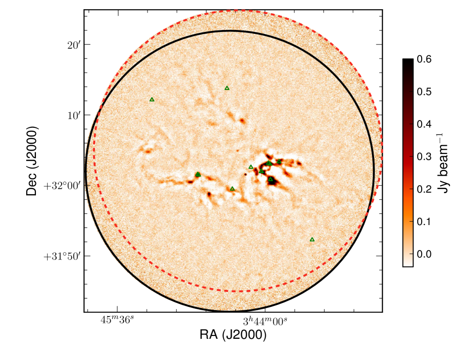
Figure 10: The Transient Survey field IC348 mosaicked with its corresponding archival GBS fields at 850 $\mu$m. The area of each observed GBS and Transient Survey field included in the mosaic is bounded by a circle. The solid black circle is the Transient Survey field. The red (dashed) circle shows the boundary of the IC348-E GBS field. The green triangles represent the positions of known protostars taken from the Spitzer Space Telescope catalogue of Dunham et al. (2015).

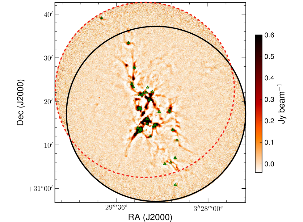
Figure 11: Same as Figure 10, but showing the NGC1333 field with its corresponding archival GBS field. The red (dashed) circle shows the NGC1333-N GBS field.

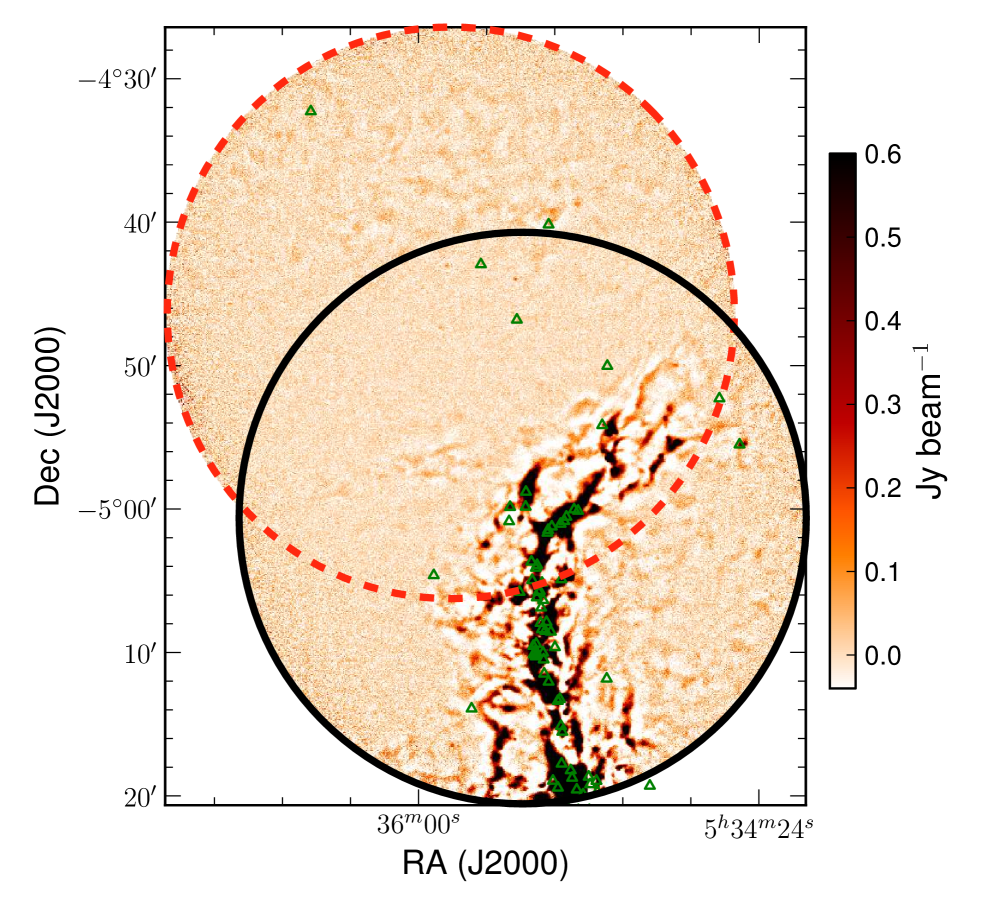
Figure 12: Same as Figure 10, but showing the OMC 2-3 field with its corresponding archival GBS fields. The red (dashed) circle shows the OMC1 tile4 GBS field. The green triangles represent the positions of known protostars taken from the Spitzer Space Telescope and Herschel Space Observatory catalogues of Megeath et al. (2012) and Stutz et al. (2013), respectively.

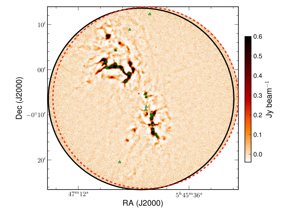
Figure 13: Same as Figure 10, but showing the NGC2068 field with its corresponding archival GBS field. The red (dashed) circle shows the ORIONBN_450_S GBS field. The green triangles represent the positions of known protostars taken from the Spitzer Space Telescope and Herschel Space Observatory catalogues of Megeath et al. (2012) and Stutz et al. (2013), respectively.

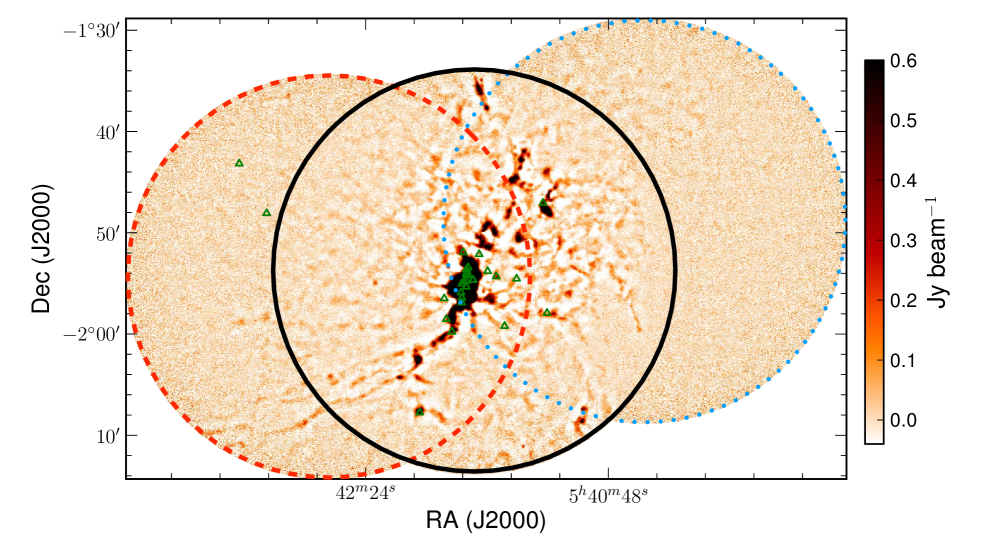
Figure 14: Same as Figure 10, but showing the NGC2024 field with its corresponding archival GBS fields. The red (dashed) circle shows the ORIONBS_450_E GBS field while the blue (dotted) circle shows the ORIONBS_450_W GBS field. The green triangles represent the positions of known protostars taken from the Spitzer Space Telescope and Herschel Space Observatory catalogues of Megeath et al. (2012) and Stutz et al. (2013), respectively.

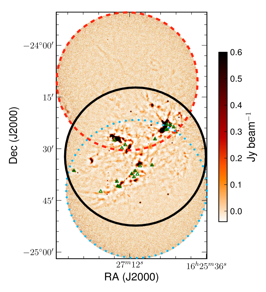
Figure 15: Same as Figure 10, but showing the Oph Core field with its corresponding archival GBS field. The red (dashed) circle shows the L1688-2 GBS field while the blue (dotted) circle shows the L1688-1 GBS field.

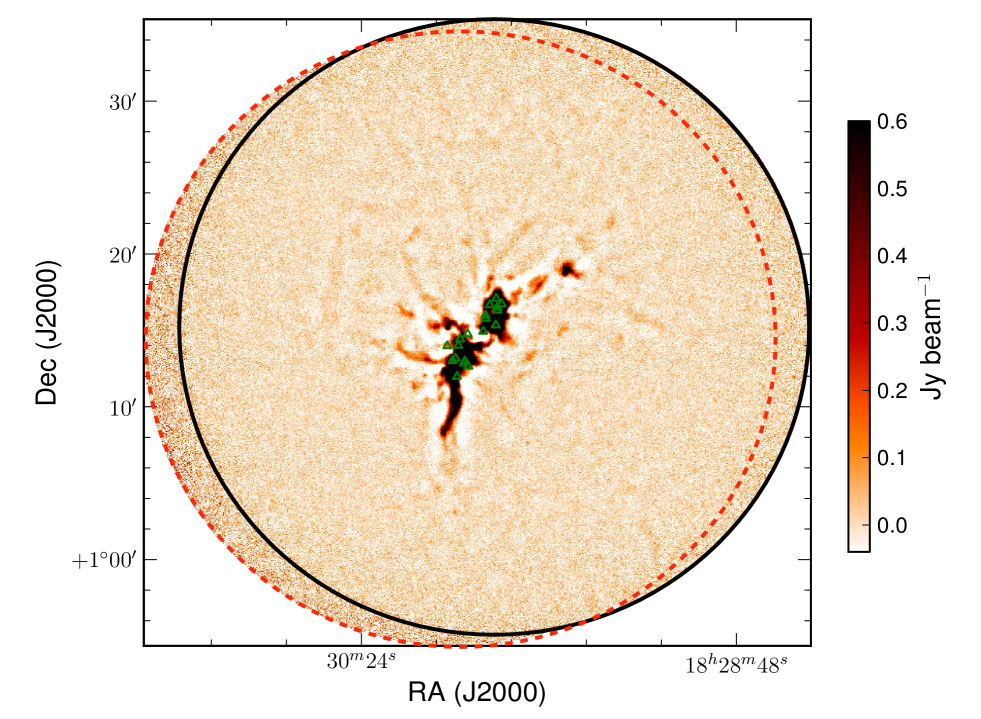
Figure 16: Same as Figure 10, but showing the Serpens Main field with its corresponding archival GBS field. The red (dashed) circle shows the SerpensMain1 GBS field.

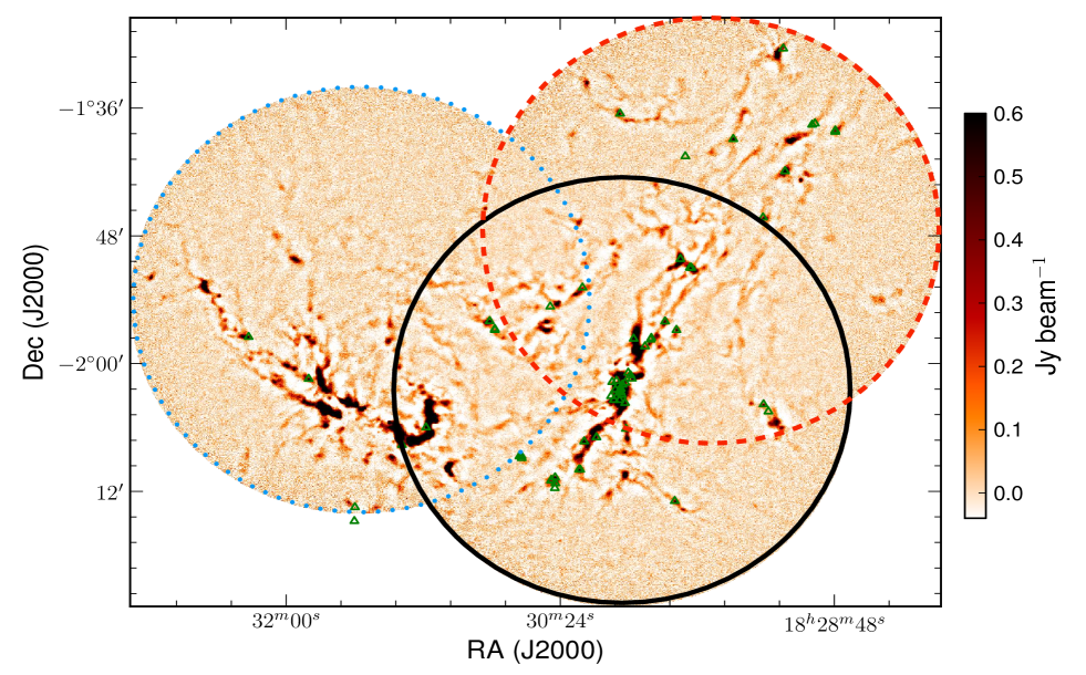
Figure 17: Same as Figure 10, but showing the Serpens South field with its corresponding archival GBS fields. The red (dashed) circle shows the SerpensS-NW GBS field while the blue (dotted) circle shows the SerpensSouthS-NE GBS field.

For maximum consistency in relative flux calibration across all the regions, we select individual GBS fields and compare each one to its respective Transient Survey field independently. For a given GBS field to be useful for this work, it must: 1) have enough bright, compact sources to undergo self calibration and 2) have significant overlap with a Transient field such that they share at least three sources of interest and a flux calibration between the two datasets can be performed. The first criterion generally causes GBS fields with some Transient field overlap to fail. In order for a specific GBS field to undergo relative flux calibration, we require at least two compact sources brighter than 0.5 Jy beam^-1 that are observed to have consistent peak brightnesses with respect to one another across all observations. If two potential calibrator sources are noted, but display discordant flux calibration factors, it is unclear which, if either, of the sources represents the more correct value without further investigation. Where we lack robust sources, we discard the field. Similarly, if only one potential calibrator source is noted, it is unclear whether or not that source is intrinsically variable and, again, we discard the field. A self-calibration failure is generally encountered when the field is very sparse, or when a field is inundated with complex, extended emission without isolated, well-defined point-like sources. In the latter case, the Gaussclumps algorithm has difficulties in defining source boundaries and properly subtracting background emission (see, for example, the “Integral Shaped Filament” in the OMC 2-3 region in Figure 12; two GBS fields with the southern extension of the filament present along the noisy edge of their field of view were discarded).

Note that a clear example of Gaussclumps having difficulty subtracting the background is in the ORIONBS_450_E field. The error bars for many sources in Figure 2 (bottom left) are large due to the inconsistency of the identified source boundaries. To appear in Figures 2 through 2, a source must be consistently observed in at least 2 GBS observations and at least 2 Transient Survey observations. Recall that we apply minimum peak brightness and maximum radius thresholds. Sources that have sizes that are near this threshold may be culled from many observations, yet detected in two or three as the extraction algorithm fits a slightly different Gaussian model to the same region on different dates, attempting to separate clustered structure. The lack of robust observations increases the uncertainty of the peak measurement but this is mitigated by well-defined, well recovered sources in conjunction with the calculation of a weighted mean to derive the relative FCF.

Source recovery in particularly confused and blended emission regions is also complicated by the fact that the recovery of extended background emission can vary from observation to observation, especially near the edges of the map. Reducing SCUBA-2 data is a complex process. Best practices for the GBS data reduction were developed by Mairs et al. (2015) and extended to the Transient Survey by Mairs et al. (2017). Adopting the methodology of Mairs et al. (2017) in this paper, we robustly recover compact structure in exchange for less information at extended scales. As discussed in Section 3.1, we perform a two-stage reduction where we employ an external mask in the final stage to help constrain makemap’s solution. These external masks are created individually for each field in the GBS and Transient surveys, due to the different central coordinates of the overlapping fields. Where the fields from the two surveys overlap (see Figures 10 through 17), the masked structures are nearly identical. Outside of these regions, however, the fields have their own structure that can slightly affect how astronomical signal across the rest of the recovered image grows in the final iteration of makemap. This effect is generally insignificant across the majority of the image but can cause slight differences near the edges of the fields where the noise levels are higher.

In many instances, the edges of GBS fields overlap with the centre of their associated Transient Survey field and the small differences in extended structure recovery create flux pedestals and negative bowling, which add to the uncertainty of a measured source in those regions (see Mairs et al., 2015, for more information). Since the telescope has to slow down and speed up near the edges, the time domain filtering has a different effect on structure near the edge of the map with respect to that at the centre of the map. We have addressed this by inspecting each of the variable candidate sources in Table 2 in difference maps we constructed (see Figures 2 and 19), looking for indications of larger-scale residual structures. We expect that compact, truly varying sources would show significant, point-like structure even in the midst of these extended regions.

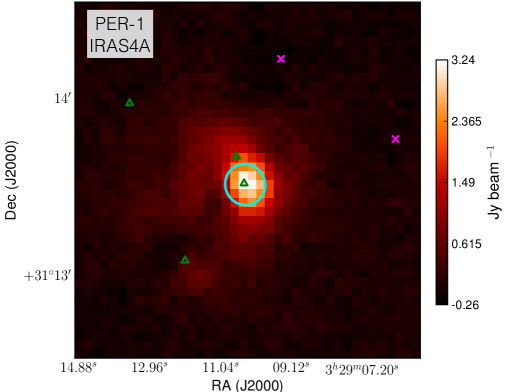
(a)

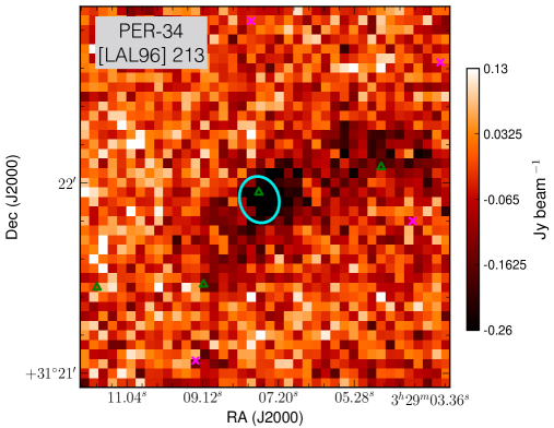
(c)

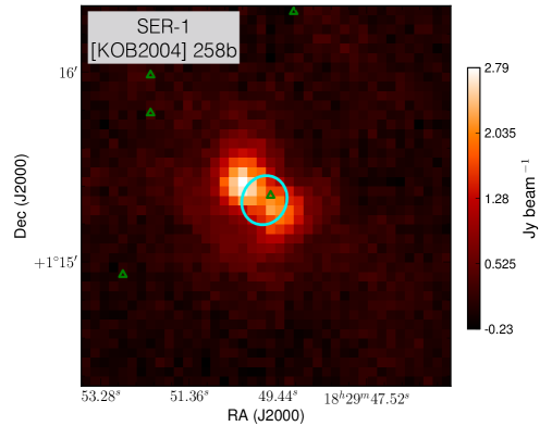
(d)

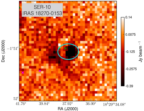
(e)

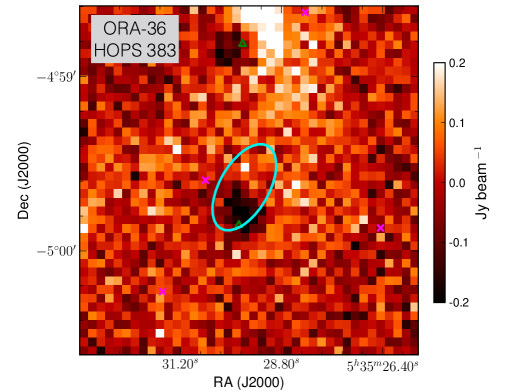
(f)

Figure 18: The 5 Strong variable candidates and the 1 Possible variable candidate (ORA-36/HOPS 383) extracted from difference maps where the GBS co-add has been subtracted from the Transient Survey co-add. Green triangles represent known protostars and magenta crosses represent known disk sources taken from the catalogues of Megeath et al. (2012), Stutz et al. (2013), and Dunham et al. (2015). Cyan boundaries show the fitted 2D Gaussian truncated at the level of 0.5$\sigma_{rms}$.

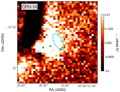
(a)

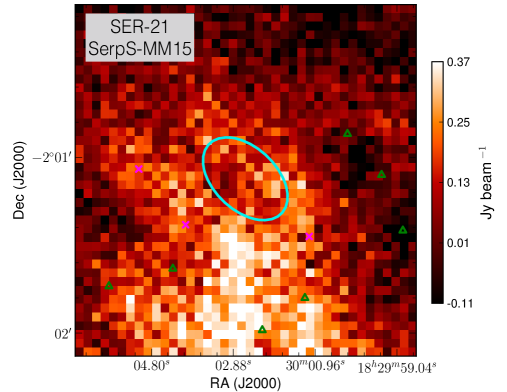
(b)

Figure 19: Same as Figure 2, but for Extended variable candidates.

In Figures 2 and 19, we present thumbnail images extracted from the constructed difference maps (the GBS co-added data subtracted from the Transient Survey co-added data) for all variable candidates in Table 2. All of the Strong variable candidates show significant, compact structure in their respective difference maps.

References

- Alencar et al. (2001) Alencar, S. H. P., Johns-Krull, C. M., & Basri, G. 2001, AJ, 122, 3335
- Andre et al. (1993) Andre, P., Ward-Thompson, D., & Barsony, M. 1993, ApJ, 406, 122
- Armitage et al. (2001) Armitage, P. J., Livio, M., & Pringle, J. E. 2001, MNRAS, 324, 705
- Astropy Collaboration et al. (2013) Astropy Collaboration, Robitaille, T. P., Tollerud, E. J., et al. 2013, A&A, 558, A33
- Audard et al. (2014) Audard, M., Ábrahám, P., Dunham, M. M., et al. 2014, Protostars and Planets VI, 387
- Avila et al. (2001) Avila, R., Rodríguez, L. F., & Curiel, S. 2001, RevMexAA, 37, 201
- Bae et al. (2014) Bae, J., Hartmann, L., Zhu, Z., & Nelson, R. P. 2014, ApJ, 795, 61
- Bae et al. (2016) Bae, J., Nelson, R. P., & Hartmann, L. 2016, ApJ, 833, 126
- Bell & Lin (1994) Bell, K. R., & Lin, D. N. C. 1994, ApJ, 427, 987
- Berry et al. (2007) Berry, D. S., Reinhold, K., Jenness, T., & Economou, F. 2007, in Astronomical Society of the Pacific Conference Series, Vol. 376, Astronomical Data Analysis Software and Systems XVI, ed. R. A. Shaw, F. Hill, & D. J. Bell, 425
- Blinova et al. (2016) Blinova, A. A., Romanova, M. M., & Lovelace, R. V. E. 2016, MNRAS, 459, 2354
- Bouvier et al. (2007) Bouvier, J., Alencar, S. H. P., Harries, T. J., Johns-Krull, C. M., & Romanova, M. M. 2007, Protostars and Planets V, 479
- Cernicharo & Reipurth (1996) Cernicharo, J., & Reipurth, B. 1996, ApJL, 460, L57
- Chapin et al. (2013) Chapin, E. L., Berry, D. S., Gibb, A. G., et al. 2013, MNRAS, 430, 2545
- Choi (2001) Choi, M. 2001, ApJ, 553, 219
- Choi et al. (2006) Choi, M., Hodapp, K. W., Hayashi, M., et al. 2006, ApJ, 646, 1050
- Cody et al. (2017) Cody, A. M., Hillenbrand, L. A., David, T. J., et al. 2017, ApJ, 836, 41
- Connelley & Greene (2010) Connelley, M. S., & Greene, T. P. 2010, AJ, 140, 1214
- Connelley et al. (2007) Connelley, M. S., Reipurth, B., & Tokunaga, A. T. 2007, AJ, 133, 1528
- Coudé et al. (2016) Coudé, S., Bastien, P., Kirk, H., et al. 2016, MNRAS, 457, 2139
- Currie et al. (2014) Currie, M. J., Berry, D. S., Jenness, T., et al. 2014, in Astronomical Society of the Pacific Conference Series, Vol. 485, Astronomical Data Analysis Software and Systems XXIII, ed. N. Manset & P. Forshay, 391
- Dempsey et al. (2013) Dempsey, J. T., Friberg, P., Jenness, T., et al. 2013, MNRAS, 430, 2534
- Di Francesco et al. (2008) Di Francesco, J., Johnstone, D., Kirk, H., MacKenzie, T., & Ledwosinska, E. 2008, ApJS, 175, 277
- Donati et al. (2013) Donati, J.-F., Gregory, S. G., Alencar, S. H. P., et al. 2013, MNRAS, 436, 881
- Drabek et al. (2012) Drabek, E., Hatchell, J., Friberg, P., et al. 2012, MNRAS, 426, 23
- Dunham & Vorobyov (2012) Dunham, M. M., & Vorobyov, E. I. 2012, ApJ, 747, 52
- Dunham et al. (2015) Dunham, M. M., Allen, L. E., Evans, II, N. J., et al. 2015, ApJS, 220, 11
- Eiroa & Casali (1992) Eiroa, C., & Casali, M. M. 1992, A&A, 262, 468
- Enoch et al. (2006) Enoch, M. L., Young, K. E., Glenn, J., et al. 2006, ApJ, 638, 293
- Evans et al. (2009) Evans, II, N. J., Dunham, M. M., Jørgensen, J. K., et al. 2009, ApJS, 181, 321
- Fischer & Hillenbrand (2017) Fischer, W. J., & Hillenbrand, L. 2017, The Astronomer’s Telegram, 9969
- Fischer et al. (2017) Fischer, W. J., Megeath, S. T., Furlan, E., et al. 2017, ApJ, 840, 69
- Forbrich et al. (2011) Forbrich, J., Osten, R. A., & Wolk, S. J. 2011, ApJ, 736, 25
- Forgan & Rice (2010) Forgan, D., & Rice, K. 2010, MNRAS, 402, 1349
- Greene & Lada (1996) Greene, T. P., & Lada, C. J. 1996, AJ, 112, 2184
- Greene et al. (1994) Greene, T. P., Wilking, B. A., Andre, P., Young, E. T., & Lada, C. J. 1994, ApJ, 434, 614
- Hartmann et al. (2016) Hartmann, L., Herczeg, G., & Calvet, N. 2016, ARAA, 54, 135
- Hartmann & Kenyon (1985) Hartmann, L., & Kenyon, S. J. 1985, ApJ, 299, 462
- Heiderman & Evans (2015) Heiderman, A., & Evans, II, N. J. 2015, ApJ, 806, 231
- Herbig (1977) Herbig, G. H. 1977, ApJ, 217, 693
- Herbig (1989) Herbig, G. H. 1989, in European Southern Observatory Conference and Workshop Proceedings, Vol. 33, European Southern Observatory Conference and Workshop Proceedings, ed. B. Reipurth, 233–246
- Herczeg et al. (2017) Herczeg, G. J., Johnstone, D., Mairs, S., et al. 2017, ArXiv e-prints, arXiv:1709.02052
- Hodapp et al. (2012) Hodapp, K. W., Chini, R., Watermann, R., & Lemke, R. 2012, ApJ, 744, 56
- Holland et al. (2013) Holland, W. S., Bintley, D., Chapin, E. L., et al. 2013, MNRAS, 430, 2513
- Hunter (2007) Hunter, J. D. 2007, Computing In Science & Engineering, 9, 90
- Jenness et al. (2013) Jenness, T., Chapin, E. L., Berry, D. S., et al. 2013, SMURF: SubMillimeter User Reduction Facility, Astrophysics Source Code Library., , , ascl:1310.007:
- Jennings et al. (1987) Jennings, R. E., Cameron, D. H. M., Cudlip, W., & Hirst, C. J. 1987, MNRAS, 226, 461
- Johns & Basri (1995) Johns, C. M., & Basri, G. 1995, ApJ, 449, 341
- Johnstone & Bally (1999) Johnstone, D., & Bally, J. 1999, ApJL, 510, L49
- Johnstone et al. (2001) Johnstone, D., Fich, M., Mitchell, G. F., & Moriarty-Schieven, G. 2001, ApJ, 559, 307
- Johnstone et al. (2013) Johnstone, D., Hendricks, B., Herczeg, G. J., & Bruderer, S. 2013, ApJ, 765, 133
- Johnstone et al. (2000) Johnstone, D., Wilson, C. D., Moriarty-Schieven, G., et al. 2000, ApJ, 545, 327
- Kaas et al. (2004) Kaas, A. A., Olofsson, G., Bontemps, S., et al. 2004, A&A, 421, 623
- Kackley et al. (2010) Kackley, R., Scott, D., Chapin, E., & Friberg, P. 2010, in Proc. SPIE, ed. T. G. Phillips & J. Zmuidzinas, Vol. 7740, 1. SPIE, Bellingham, WA
- Kenyon et al. (1990) Kenyon, S. J., Hartmann, L. W., Strom, K. M., & Strom, S. E. 1990, AJ, 99, 869
- Kirk et al. (2006) Kirk, H., Johnstone, D., & Di Francesco, J. 2006, ApJ, 646, 1009
- Lada et al. (1996) Lada, C. J., Alves, J., & Lada, E. A. 1996, AJ, 111, 1964
- Mairs et al. (2015) Mairs, S., Johnstone, D., Kirk, H., et al. 2015, MNRAS, 454, 2557
- Mairs et al. (2016) —. 2016, MNRAS, 461, 4022
- Mairs et al. (2017) Mairs, S., Lane, J., Johnstone, D., et al. 2017, ApJ, 843, 55
- Maury et al. (2011) Maury, A. J., André, P., Men’shchikov, A., Könyves, V., & Bontemps, S. 2011, A&A, 535, A77
- McKee & Offner (2011) McKee, C. F., & Offner, S. R. R. 2011, in IAU Symposium, Vol. 270, Computational Star Formation, ed. J. Alves, B. G. Elmegreen, J. M. Girart, & V. Trimble, 73–80
- Megeath et al. (2012) Megeath, S. T., Gutermuth, R., Muzerolle, J., et al. 2012, AJ, 144, 192
- Meixner et al. (2016) Meixner, M., Cooray, A., Carter, R., et al. 2016, in Proc. SPIE, Vol. 9904, Space Telescopes and Instrumentation 2016: Optical, Infrared, and Millimeter Wave, 99040K
- Nayakshin & Lodato (2012) Nayakshin, S., & Lodato, G. 2012, MNRAS, 426, 70
- Reipurth (1989) Reipurth, B. 1989, A&A, 220, 249
- Reipurth (1990) Reipurth, B. 1990, in IAU Symposium, Vol. 137, Flare Stars in Star Clusters, Associations and the Solar Vicinity, ed. L. V. Mirzoian, B. R. Pettersen, & M. K. Tsvetkov, 229–251
- Reipurth et al. (2004) Reipurth, B., Rodríguez, L. F., Anglada, G., & Bally, J. 2004, AJ, 127, 1736
- Ribas et al. (2015) Ribas, Á., Bouy, H., & Merín, B. 2015, A&A, 576, A52
- Rice et al. (2010) Rice, W. K. M., Mayo, J. H., & Armitage, P. J. 2010, MNRAS, 402, 1740
- Robitaille & Bressert (2012) Robitaille, T., & Bressert, E. 2012, APLpy: Astronomical Plotting Library in Python, Astrophysics Source Code Library, , , ascl:1208.017
- Romanova et al. (2003) Romanova, M. M., Toropina, O. D., Toropin, Y. M., & Lovelace, R. V. E. 2003, ApJ, 588, 400
- Safron et al. (2015) Safron, E. J., Fischer, W. J., Megeath, S. T., et al. 2015, ApJL, 800, L5
- Santangelo et al. (2015) Santangelo, G., Codella, C., Cabrit, S., et al. 2015, A&A, 584, A126
- Shu (1977) Shu, F. H. 1977, ApJ, 214, 488
- Skrutskie et al. (2006) Skrutskie, M. F., Cutri, R. M., Stiening, R., et al. 2006, AJ, 131, 1163
- Stutz et al. (2013) Stutz, A. M., Tobin, J. J., Stanke, T., et al. 2013, ApJ, 767, 36
- Stutzki & Guesten (1990) Stutzki, J., & Guesten, R. 1990, ApJ, 356, 513
- Vorobyov & Basu (2005) Vorobyov, E. I., & Basu, S. 2005, ApJL, 633, L137
- Vorobyov & Basu (2006) —. 2006, ApJ, 650, 956
- Vorobyov & Basu (2010) —. 2010, ApJ, 719, 1896
- Vorobyov & Basu (2015) —. 2015, ApJ, 805, 115
- Ward-Thompson et al. (2007) Ward-Thompson, D., Di Francesco, J., Hatchell, J., et al. 2007, PASP, 119, 855
- Yoo et al. (2017) Yoo, H., Lee, J.-E., Mairs, S., et al. 2017, ArXiv e-prints, arXiv:1709.04096
- Zhang et al. (2015) Zhang, M., Fang, M., Wang, H., et al. 2015, ApJS, 219, 21
- Zhu et al. (2007) Zhu, Z., Hartmann, L., Calvet, N., et al. 2007, ApJ, 669, 483
- Zhu et al. (2009) Zhu, Z., Hartmann, L., & Gammie, C. 2009, ApJ, 694, 1045