Flipping-shuttle oscillations of bright one- and two-dimensional solitons in spin-orbit-coupled Bose-Einstein condensates with Rabi mixing

Abstract

We analyze a possibility of macroscopic quantum effects in the form of coupled structural oscillations and shuttle motion of bright two-component spin-orbit-coupled striped (one-dimensional, 1D) and semi-vortex (two-dimensional, 2D) matter-wave solitons, under the action of linear mixing (Rabi coupling) between the components. In 1D, the intrinsic oscillations manifest themselves as flippings between spatially even and odd components of striped solitons, while in 2D the system features periodic transitions between zero-vorticity and vortical components of semi-vortex solitons. The consideration is performed by means of a combination of analytical and numerical methods.

I Introduction

Atomic Bose-Einstein condensates (BEC), in addition to exhibiting a great deal of their own dynamical regimes BEC-book1 ; Rev1 ; Rev2 , have drawn a lot of interest as testing grounds for the emulation of various effects from condensed-matter physics emulator , a prominent example  provided by the spin-orbit coupling (SOC). Although the true spin of bosonic atoms, such as ${}^{87}\mathrm{Rb}$, used for the SOC emulation in BEC, is zero, the wave function of the condensate may be composed as a mixture of two components representing different hyperfine atomic states. The resulting  pseudospin $1/2$ makes it possible to map the spinor wave function of electrons in solids into the two-component bosonic wave function of the atomic BEC. Breakthrough experiments Nature ; soc2 have demonstrated the real possibility to simulate the SOC effect in the bosonic gas, in the form of the linear interaction between the momentum and pseudospin of coherent matter waves. Two fundamental types of the SOC, well known from works on physics of semiconductors, which are represented by the Dresselhaus Dresselhaus and Rashba Rashba Hamiltonians, as well as the Zeeman-splitting effect Campbell , may be simulated in the atomic BEC. While the initial experiments on the SOC emulation realized effectively one-dimensional (1D) settings NatureRev ; Review , the implementation of the SOC in an effectively 2D geometry was reported too 2D-experiment .

The SOC being a linear effect by itself, its interplay with the intrinsic nonlinearity of the BEC, which is usually induced, in the mean-field approximation, by contact inter-atomic collisions or long-range dipole-dipole interactions, produces various localized structures, such as vortices vortex1 ; vortex2 ; vortex3 ; SL ; vortex4 , monopoles monopole , skyrmions skyrmions2 ; skyrmions1 , and dark solitons DS2 ; DS3 . The use of periodic potentials, induced by optical lattices, offers additional possibilities – in particular, the creation of gap solitons gap-sol1 ; gap-sol2 ; gap-sol3 .

The conventional repulsive sign of inter-atomic forces can be switched to attraction by means of the Feshbach resonance Cornish ; Feshbach , which suggests possibilities for the creation of bright matter-wave solitons Rice ; Paris ; Cornish2 ; Cornish3 , in addition to the well-known dark ones DS1 . In particular, the modulational instability MI and various options for the making of effectively 1D bright solitons under the action of SOC in attractive condensates have been theoretically analyzed in detail sol1 -He . A challenging possibility is to introduce 2D bright solitons, which are always unstable against the critical collapse in the usual BEC models based on the nonlinear Schrödinger – Gross-Pitaevskii equations (NLSEs-GPEs) with attractive cubic terms Fibich . As demonstrated in Ref. Sakaguchi , the SOC terms break the specific scaling invariance of the GPE system in the 2D space, lift the related degeneracy of the norm of the respective 2D solitons, and thus push the norm below the threshold necessary for the onset of the critical collapse, securing their stability. This unique possibility to stabilize bright solitons in the free 2D space was further elaborated in Refs. Cardoso -Sherman . Furthermore, the same mechanism may create free-space metastable solitons in the 3D geometry, although in that case the solitons cannot realize the system’s ground state Pu .

In addition to the realizations of SOC in BEC, the similarity between the GPEs for the binary condensate and the NLSE system modeling the copropagation of orthogonal polarizations of light in twisted nonlinear optical fibers old ; sol2 suggests to link the SOC to a broad range of nonlinear effects in optics. This link has been recently extended to 2D setting too optics ; NJP , making it possible to predict stable spatiotemporal optical solitons in planar dual-core waveguides. Manifestations of SOC are also known in other photonic settings Bliokh . In particular, SOC can be directly realized in exciton-polariton fields trapped in semiconductor microcavities cavity . Taking into regard nonlinearity in the latter setting makes it possible to predict 2D trapped modes similar to the solitons found in the 2D model of the BEC with SOC Dmitry .

A common feature of 1D and 2D bright solitons supported by the attractive nonlinearity in the two-component system coupled by the spin-orbit interaction is the different shape of solitons in the cases when the XPM/SPM ratio (the relative strength of the cross-attraction and self-attraction), $\gamma$, takes values $\gamma\leq 1$ or $\gamma\geq 1$. In the former case, the 1D system produces stable striped solitons (see, e.g., Ref. we ), built as patterns featuring multiple density peaks in the two components, with density maxima of one component coinciding with minima of the other. Accordingly, the two components of the striped solitons feature opposite spatial parities, one being even and the other odd. In the case of $\gamma\geq 1$, stable 1D solitons feature a smooth single-peak density profile, identical for both components. Similarly, the 2D system with $\gamma\leq 1$ supports semi-vortex (SV) solitons as stable modes, with isotropic components which carry, respectively, vorticities $0$ and $1$, while stable solitons produced by the same system with $\gamma\geq 1$ are mixed modes, which combine terms with zero and nonzero vorticities in each component Sakaguchi . Precisely at $\gamma=1$ (the Manakov’s nonlinearity Manakov ), solitons of both types stably coexist Sakaguchi ; we .

Because bright matter-wave solitons, predicted and observed in BEC, are macroscopic quantum objects, the consideration of the overall dynamics of solitons in binary condensates under the action of SOC suggests a possibility to observe macroscopic manifestations of SOC. An example is provided by recent work Beijing , in which an artificial magnetic field, induced by the SOC terms in the 1D system, drives precession of the soliton’s pseudospin, which, in turn, drives shuttle motion of the 1D soliton as a whole. Prior to that, coupling of the precession of the total pseudospin to the motion of a dark soliton in a ring-shaped effectively one-dimensional SOC system was predicted in Ref. Brand .

The objective of the present work is to report another kind of macroscopic dynamical effects featured by 1D and 2D solitons alike, under the combined action of the SOC and Rabi coupling (RC). These effect exhibit periodic flippings between the two components of the condensate, coupled to the shuttle motion of the soliton’s center, with the same period. In the 1D system, these are flippings between spatially even and odd components of striped solitons, while in the 2D setting the vorticity is periodically exchanged between two components of the SV soliton, if the motion of the soliton is restricted in one direction by a quasi-1D confining potential. The latter dynamical effect somewhat resembles periodic transfer of a single vortex between two Rabi-coupled components of a 2D condensate, with the repulsive nonlinearity acting in each component AFetter , although in that case the mode periodically exchanged between the components is not a bright soliton, but rather a vortex supported by the modulationally stable background. As for the RC, it represents linear mixing between two hyperfine atomic states (which constitute the two components), induced by a resonant electromagnetic (GHz-frequency) wave coupling the atomic levels RC1 -RC5 .

The rest of the paper is organized as follows. The flipping-shuttle motion of 1D solitons in considered, by means of analytical approximations and systematic simulations, in Section II. The regime of periodic flippings between the 2D SV soliton and its mirror-image counterpart, coupled to the shuttle motion of the soliton as a whole in the direction which is not restricted by the confining potential, is investigated, chiefly by means of numerical simulations, in Section III. It is also shown that the use of an isotropic trapping potential, instead of the quasi-1D one, leads to chaotic dynamics, instead of regular flipping-shuttle motion. The paper is concluded by Section IV.

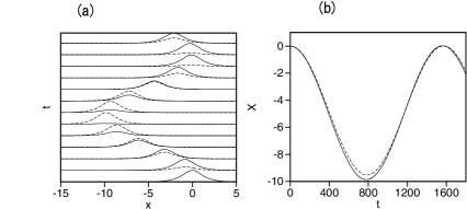
Figure 1: (a) Snapshots of components $|\phi_{+}(x)|$ and $|\phi_{-}(x)|$ of the 1D soliton (shown by continuous and dashed lines, respectively) at $t=150\times n$ ($n=1,2,\cdots,12$). (b) The continuous line depicts the motion of the soliton’s center of mass, $X(t)$, for $\lambda=0.02$, $d=0.002$, $\gamma=1$, and total norm $N=2$, see Eq. (3). The dashed line is the analytical prediction given by Eq. (17).

II Flipping-shuttle dynamics of one-dimensional solitons

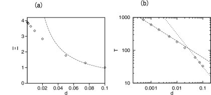
Figure 2: (a) Half-amplitude $\Xi$ of the shuttle motion vs. the Rabi-coupling strength, $d$, at $\lambda=0.2$, $\gamma=1$, and $N=2$. The dashed line is the analytical prediction $\Xi=(10/21)(\lambda/d)$ given by Eq. (18). (b) The period of the flipping-shuttle oscillations vs. $d$ at $\lambda=0.2$, $\gamma=1$, and $N=2$. The dotted line is $\pi/d$, which corresponds to Eq. (17), while the dashed line is $19/d^{1/2}$.

We consider the GPE system with SOC terms of the Rashba type and RC, which is written in a scaled form as

$$i\frac{\partial\phi_{+}}{\partial t} = -\frac{1}{2}\frac{\partial^{2}\phi_{+}}{\partial x^{2}}-(|\phi_{+}|^{2}+\gamma|\phi_{-}|^{2})\phi_{+}+\lambda\frac{\partial\phi_{-}}{\partial x}-d\phi_{-},$$

$$i\frac{\partial\phi_{-}}{\partial t} = -\frac{1}{2}\frac{\partial^{2}\phi_{-}}{\partial x^{2}}-(|\phi_{-}|^{2}+\gamma|\phi_{+}|^{2})\phi_{-}-\lambda\frac{\partial\phi_{+}}{\partial x}-d\phi_{+},$$

where $\gamma$ is the above-mentioned relative strength of the inter-component attraction, with respect to the self-attraction. Previous works, which addressed this system in the absence of the RC ($d=0$), have revealed striped bright solitons, composed of alternating segments occupied by the two components (with opposite parities, even and odd), at $\gamma<1$, and smooth solitons, with $\left|\phi_{+}(x)\right|=\left|\phi_{-}(x)\right|$, at $\gamma>1$ we . In fact, scattering lengths of interactions between atoms which represent different components of the pseudo-spinor wave function are almost exactly equal Ho , therefore we focus below, chiefly, on the case of $\gamma=1$, which corresponds the Manakov’s nonlinearity, in terms of optics models Manakov (nevertheless, the case of $\gamma\neq 1$ is briefly considered too, see Fig. 5 below). If SOC is absent ($\lambda=0$), the 1D Manakov’s system is integrable, including the case when the RC terms are present Tratnik . In the latter case, it is easy to find an exact bright-soliton solution with Rabi oscillations between the components:

$$\phi_{+}=\frac{A\cos(dt)e^{iA^{2}t/2}}{\cosh(Ax)},\;\phi_{-}=\frac{iA\sin(dt)e^{iA^{2}t/2}}{\cosh(Ax)}.$$ (2)

The total norm and energy of the general 1D system (LABEL:1DSOC), which includes the SOC and RC terms, are

$$N=\int_{-\infty}^{+\infty}\left(\left|\phi_{+}(x)\right|^{2}+\left|\phi_{-}(x)\right|^{2}\right)dx,$$ (3)

$$E=\int_{-\infty}^{+\infty}\left\{\frac{1}{2}\left(\frac{\partial\phi_{+}}{\partial x}\right)^{2}+\frac{1}{2}\left(\frac{\partial\phi_{-}}{\partial x}\right)^{2}-\frac{1}{2}\left(|\phi_{+}|^{2}+|\phi_{-}|^{2}\right)^{2}+\frac{\lambda}{2}\left(\phi_{+}^{\ast}\frac{\partial\phi_{-}}{\partial x}-\phi_{-}^{\ast}\frac{\partial\phi_{+}}{\partial x}+\mathrm{c.c.}\right)\right\}dx,$$ (4)

where $\mathrm{c.c.}$ stands for the complex-conjugate expression. When RC is absent, $d=0$, and SOC is weak, i.e., $\lambda$ is small, an approximate solution to Eq. (LABEL:1DSOC) with a large even component, $\phi_{+}$, and a small odd one, $\phi_{\_}$ (these assumptions are suggested by the presence of the weak SOC terms), may be sought for as

$$\phi_{+}=\frac{Ae^{iA^{2}t/2}}{\cosh(Ax)},\;\phi_{-}=\frac{B\sinh(Ax)e^{iA^{2}t/2}}{\cosh^{2}(Ax)},$$ (5)

with $B^{2}\ll A^{2}$. The substitution of this ansatz in Eq. (4) yields

$$E=\frac{7}{15}AB^{2}-\frac{B^{4}}{35A}+\frac{4}{3}\lambda AB-\frac{1}{3}A^{3}.$$ (6)

For given $A$ and small $\lambda$, the corresponding small amplitude $B$ is predicted by the variational equation $\partial E/\partial B=0$:

$$B=(-10/7)\lambda+O\left(\lambda^{2}/A^{2}\right).$$ (7)

Proceeding to simulations of the full GPE system (LABEL:1DSOC), but, at first, with small SOC and RC terms, Figs. 1(a) and (b) show, respectively, snapshots of profiles of $|\phi_{+}(x)|$ and $|\phi_{-}(x)|$ at time moments $t=150\times n$ ($n=1,2,\cdots,12$), and the corresponding numerically found law of motion of the soliton’s center-of-mass coordinate, $X(t)$, obtained for parameters $d=0.002$, $\lambda=0.02$, $\gamma=1$ and $N=2$. For these simulations, initial conditions, $\phi_{+}(x,t=0)$ and $\phi_{-}(x,t=0)$, were produced as stationary solutions of Eq. (LABEL:1DSOC) with $d=0$ (but $\lambda\neq 0$), by dint of the imaginary-time-evolution method. Due to the presence of the SOC terms, the two components have opposite spatial parities: $\phi_{+}(-x,t=0)=\phi_{+}(x,t=0),~{}\phi_{-}(-x,t=0)=-\phi_{-}(x,t=0)$. Thus, Fig. 1 demonstrates that, at $d\neq 0$, shuttle motion appears, coupled to flipping oscillations. For an analytical consideration of this dynamical regime, we adopt an ansatz in the form which is also suggested by exact solution (2) of the Manakov’s system, but, unlike the above ansatz (5), this time it combines expressions modeled on solution (2) in both components:

$$\left(\begin{array}[]{c}\phi_{+}\\ \phi_{-}\end{array}\right)=\exp\left[i\frac{A^{2}}{2}t+i\frac{d\xi}{dt}\left(x-\xi\right)\right]\mathrm{sech}\left[A(x-\xi)\right]$$ (10)

$$\times\left(\begin{array}[]{c}A\cos(dt)-iB\sin(dt)\tanh\left[A(x-\xi)\right]\\ iA\sin(dt)+B\cos(dt)\tanh\left[A(x-\xi)\right]\end{array}\right),$$ (13)

where $\xi(t)$ is the central position of the soliton. Then, applying the variational approximation to this system leads, eventually, to the same relation (7) between the small and large amplitudes, $A$ and $B$.

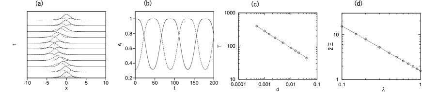
Figure 3: (a) The evolution of components $|\phi_{+}(x)|$ and $|\phi_{-}(x)|$ (solid and dashed lines) produced by simulations of the 1D system (LABEL:1DSOC) with $\gamma=1$, $d=0.01$, $\lambda=0.5$, and $N=2$. (b) Amplitudes of $|\phi_{+}(x)|$ and $\left|\phi_{-}(x)\right|$(solid and dashed curves, respectively) as functions of time. (c) Period $T$ of the shuttle-flipping oscillaltions vs. the Rabi-coupling coefficient, $d$, shown on the log-log scale, for $N=2$ and $\lambda=0.5$. The dashed line is $T=8.9d^{-1/2}$. (d) The amplitude of the shuttle motion, $2\Xi$, vs. the SOC coefficient, $\lambda$, on the log-log scale, for $N=2$ and $d=0.005$. The dashed line is $2\Xi=1.56\lambda^{-1}$.

Further, to address the motion of the soliton as a whole, it is relevant to consider the total momentum of the system,

$$P=i\int_{-\infty}^{+\infty}\left(\frac{\partial\phi_{+}^{\ast}}{\partial x}\phi_{+}+\frac{\partial\phi_{-}^{\ast}}{\partial x}\phi_{-}\right)dx.$$ (14)

Being a dynamical invariant of Eq. (LABEL:1DSOC), $P$ keeps zero initial value. On the other hand, ansatz (13), if substituted in Eq. (14), produces

$$P=-\frac{4}{3}AB\sin(dt)\cos(dt)+2\left(A+\frac{B^{2}}{3A}\right)\frac{d\xi}{dt}.$$ (15)

Finally, substituting $B$, as given by Eq. (7) for sufficiently small $\lambda$, in the momentum-conservation condition $P=0$ following from Eq. (15), leads to the prediction for the velocity of the moving soliton:

$$\frac{d\xi}{dt}=-\frac{20}{21}\lambda\sin(2dt).$$ (16)

A solution of this equation, satisfying the initial condition $\xi(0)=0$, is

$$\xi(t)=-\Xi_{\mathrm{pert}}\left[1-\cos(2dt)\right],$$ (17)

$$\Xi_{\mathrm{pert}}=\left(10/21\right)\left(\lambda/d\right).$$ (18)

Direct simulations of Eq. (LABEL:1DSOC), performed at sufficiently small $\lambda$, produce the shuttle motion of the soliton’s center-of-mass coordinate

$$X=N^{-1}\int_{-\infty}^{+\infty}x(|\phi_{+}|^{2}+|\phi_{-}|^{2})dx,$$ (19)

which is very close to analytical prediction (17), as seen in Fig. 1(b).

Figure 2(a) shows numerically evaluated half-amplitude of the shuttle oscillations, $\Xi$ and its perturbative prediction (the dashed line), given by Eq. (18), for $\lambda=0.2$, $\gamma=1$, and $N=2$. Figure 2(b) shows the numerically found period of the flipping-shuttle oscillations, $T$ and its perturbative prediction, $\pi/d$ (the dotted line), for the same parameters. They demonstrate that the predictions are fairly good unless the RC strength, $d$, becomes too small (roughly, smaller than $\lambda/L$, where $L$ is a characteristic width of the soliton), when it must be treated as a perturbation, see below [note that, to derive Eq. (16), the RC terms were taken into account not perturbatively but as leading ones, while the SOC was treated as a perturbation].

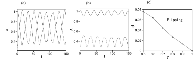
Figure 4: (a) The evolution of amplitudes of components $|\phi_{+}|$ and $\left|\phi_{-}\right|$ (solid and dashed curves), at $d=0.1$, $\gamma=0.5$, $\lambda=0.5$, and $N=2$. (b) The same, but at $d=0.05$. In the former case, flippings take place, while in the latter one flippings are suppressed. (c) The smallest value of $d$, at which flippings commence (for $\lambda=0.5$, $N=2$), vs. $\gamma$.

For stronger SOC (larger $\lambda$), the shuttle-flipping dynamics was studied by means of systematic simulations of Eq. (LABEL:1DSOC). Figure 3(a) shows snapshot profiles of $|\phi_{+}|$ and $|\phi_{-}|$ for $\lambda=0.5$ and $d=0.01$. In this case, flipping oscillations between even and odd spatial components, accompanying the shuttle motion of the soliton as a whole (with amplitude $2\Xi=3.08$) are clearly observed. Figure 3(b) illustrates this dynamical regime by displaying the evolution of amplitudes of components $|\phi_{+}|$ and $|\phi_{-}|$. This dynamical regime may be compared to a different one, which was reported, as mentioned above, in Ref. Beijing , which addressed the 1D system with SOC of the mixed Rashba-Dresselhaus type, RC, and Zeeman detuning. In Ref. Beijing , the variational approximation and direct simulations have revealed shuttle oscillations of two-component solitons, both bright and dark ones, coupled to the rotation of their pseudo-spin vectors around the artificial magnetic field (the bright soliton suffered decay if the cubic nonlinearity was not strong enough). Getting back to the present model, we note that it also applies in fiber optics to the bimodal light propagation in a nonlinear twisted fiber (the twist accounts for the effective RC between two polarizations of light), if the phase-velocity and group-velocity birefringence are taken into regard, emulating the Zeeman splitting and SOC, respectively old . In the fiber-optics model, similar oscillations of the polarization of light, coupled to shuttle motion of the soliton’s center along the temporal coordinate, were predicted long ago old , and a related dynamical regime was proposed for the use in rocking fiber-optics filters Wabnitz .

Figure 3(c) summarizes the numerical results by showing a relationship between the period, $T$, of the flipping-shuttle oscillations and small values of the RC coefficient, $d$, at $\lambda=0.5$. The figure demonstrates scaling $T\sim d^{-1/2}$, which is clearly different from that exhibited by the exact solution (2) of the Manakov’s system, as well as by the approximate solution (17) derived by means of the perturbation theory for small $\lambda$ (while the RC terms were treated as basic ones, rather than as a perturbation), $T_{0}=\pi/d$. Scaling $T\sim d^{-1/2}$ can be explained by the fact that, if the RC represents a perturbation, while the SOC terms are included in the main part of the system (even if it is not easy to do that explicitly), the restoration force, induced by the perturbation, scales as $d$, hence the frequency of small oscillations, induced by this force, scales as $\sqrt{d}$. A global picture of the $T(d)$ dependence is depicted in Fig. 2(b), showing the crossover from $T=19/d^{1/2}$ at smaller $d$ to $T_{0}=\pi/d$ at larger $d$.

Further, Fig. 3(d) displays the dependence of amplitude $2\Xi$ of the shuttle motion on non-small values of the SOC coefficient, $\lambda$, for fixed small $d=0.005$. The dependence suggests scaling $\Xi\sim\lambda^{-1}$, which is strongly different from that in Eq. (18), derived above for small $\lambda$. This scaling can be readily explained in the limit of large $\lambda$. Indeed, as shown in Refs. NJP and Raymond , for large $\lambda$ one may neglect, in the first approximation, the kinetic-energy terms in Eq. (LABEL:1DSOC), which lends the system a quasi-Dirac spectrum with a gap, $\omega^{2}=d^{2}+\lambda^{2}k^{2}$ ($\omega$ and $k$ are the frequency and wavenumber of small excitations), keeping $\lambda^{-1}$ as the single spatial scale.

In the case of the Manakov’s nonlinearity, considered above ($\gamma=1$), flipping occurs at arbitrarily small values of the RC strength, $d$, which is explained by the fact that this form of the nonlinearity supports rotational invariance in the plane of the two components, $\left(\phi_{+},\phi_{-}\right)$, thus facilitating their mutual conversion. However, at $\gamma<1$ there is a barrier against the conversion, which prevents flippings at small $d$. Figure 4(a) illustrates this effect, showing that flippings take place at $d=0.1$ for $\gamma=0.5$, $\lambda=0.5$, and $N=2$. On the other hand, in is seen in Fig. 4(b) that flippings are suppressed at $d=0.05$ (the amplitude of $|\phi_{+}|$ always remains larger that that of $|\phi_{-}|$). The evolution displayed in Figs. 4(a) and (b) shows some irregularity at $\gamma\neq 1$, due to the fact that the evolution was initiated by the initial condition constructed as the stationary solution of Eq. (LABEL:1DSOC) with $d=0$, while the simulations were performed with $d\neq 0$. Further, Fig. 4(c) shows the critical (smallest) value of $d$ at which flippings commence. To explain the nearly linear dependence between critical $d$ and $1-\gamma$, we recall the above-mentioned argument, according to which the RC terms, if treated as a perturbation, induce a force (torque) $\sim d$ driving the linear conversion in the plane of $\left(\phi_{+},\phi_{-}\right)$. On the other hand, the barrier blocking the rotation is proportional to $1-\gamma$ (the deviation from the Manakov’s case, $\gamma=1$). The onset of flipping is determined by the equilibrium between these factors, i.e., indeed, $d\sim 1-\gamma$.

At $\gamma>1$, the 1D bright smooth solitons with $\left|\phi_{+}(x)\right|=\left|\phi_{-}(x)\right|$ have a lower energy than the striped ones (which exist at $\gamma>1$ too), and the smooth solitons do not exhibit the flipping dynamics. Nevertheless, simulations performed at $d>1$ with the input in the form of the striped solitons demonstrate that regular flipping-shuttle dynamics still occurs, as shown in Fig. 5(a) and (b) for $\gamma=1.25$, $d=0.05$, $\lambda=0.2$, and $N=2$. The increase of $\gamma$ from $1.25$ to $1.30$, and of $d$ from $0.05$ to $0.1$ leads to chaotization of the flipping dynamics, as shown in Fig. 5(c).

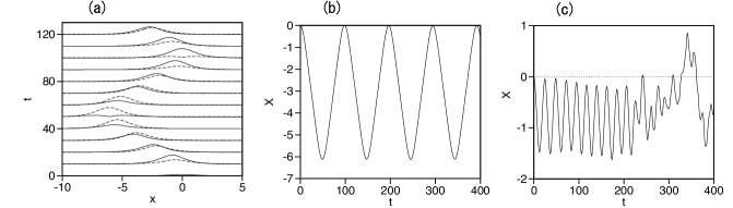
Figure 5: (a) The evolution of components $|\phi_{+}|$ and $\left|\phi_{-}\right|$ (solid and dashed curves) in the case of  $\gamma=1.25$; (b) the respective motion of the soliton’s center of mass. In this case, robust flipping-shuttle dynamics is observed at $\gamma>1$. Other parameters are $\lambda=0.2$, $d=0.05$, and $N=2$. (c) Chaotic motion of the center of mass at $d=0.1$ for $\gamma=1.3$ and $\lambda=0.2$.

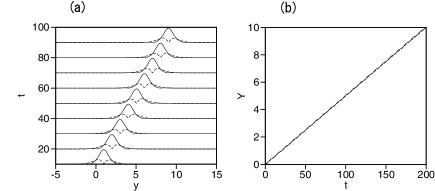
Figure 6: (a) The evolution of cross-sections $x=0$ of two-dimensional components $|\phi_{+}(x,y)|$ and $|\phi_{-}(x,y)|$ of the semi-vortex soliton (solid and dashed lines, respectively), produced as a numerical solution (semi-vortex) of Eq. (20) at $d=0.05$, $\gamma=1$, $\lambda=1$, with total 2D norm $N=5$, see Eq. (21). (b) The evolution of coordinate $Y$ of the soliton’s center, defined as per Eq. (24). The dashed line is $Y=0.05\cdot t$.

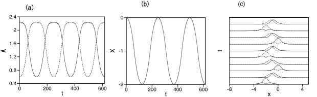
Figure 7: (a)  The evolution of amplitudes of components $|\phi_{+}\left(x,y\right)|$ and $\left|\phi_{-}\left(x,y\right)\right|$ (solid and dashed lines, respectively) of the 2D semi-vortex, obtained from simulations of Eq. (20), at $\gamma=1$, $d=0.001$, $\lambda=1$, $\Omega_{x}=0$, $\Omega_{y}=1$, and $N=5$. (b) The motion of the soliton’s center in the $y$ direction, in the course of the shuttle motion. (c) Cross-section profiles of components $|\phi_{+}\left(x,y\right)|$ and $\left|\phi_{-}\left(x,y\right)\right|$, drawn along $y=0$ (solid and dashed lines), at $t=61.5\times n$ ($n=0,1,\cdots,10$).

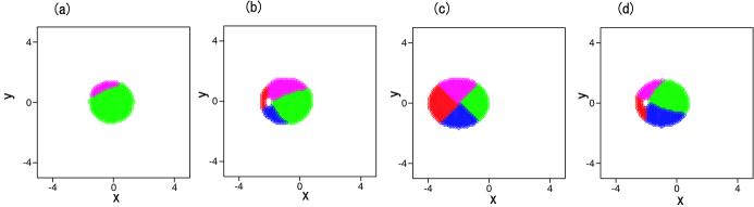
Figure 8: Four snapshot profiles of $\phi_{+}$, displayed at (a) $t=30.75$, (b) $t=61.5$, (c) $t=123$, and (d) $t=184.5$, illustrate the dynamics of the flipping evolution of a 2D semi-vortex, presented in Fig. 7. Different colors cover four regions, defined by $|\phi_{+}|>0.1$,$\;\mathrm{Re}\left(\phi_{+}\right)>0$,$\;\mathrm{Im}\left(\phi_{+}\right)>0$ (green) ; $|\phi_{+}|>0.1$,$\;\mathrm{Re}\left(\phi_{+}\right)<0$,$\;\mathrm{Im}\left(\phi_{+}\right)>0$ (blue); $|\phi_{+}|>0.1$,$\;\mathrm{Re}\left(\phi_{+}\right)<0$,$\;\mathrm{Im}\left(\phi_{+}\right)<0$ (red); $|\phi_{+}|>0.1$,$\;\mathrm{Re}\left(\phi_{+}\right)>0$,$\;\mathrm{Im}\left(\phi_{+}\right)<0$ (purple). The junction point of the four colors (sometimes seen as a while dot) is the pivot of the vortex, which enters the zero-vorticity component from outside through the edge, attains the central position, and then moves backwards, exiting the component through the same edge.

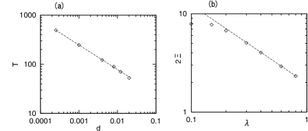
Figure 9: (a) The period of the flipping-shuttle motion of a robust 2D semivortex vs. $d$ at $\lambda=1$. (b) The amplitude $2\Xi$ vs. $\lambda$ of the shuttle motion at $d=0.01$. Other parameters are the same as in Fig. 7.

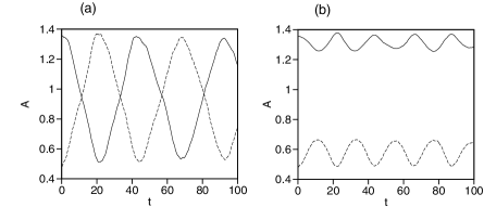
Figure 10: The evolution of amplitudes of components $|\phi_{+}\left(x,y\right)|$ and $\left|\phi_{-}\left(x,y\right)\right|$(solid and dashed lines, respectively) of the 2D semi-vortex soliton at $d=0.1$ (a) and $d=0.05$ (b). Other parameters are $\gamma=0$, $\lambda=1$, $\Omega_{x}=0$, $\Omega_{y}=1$, and $N=4$, in both cases.

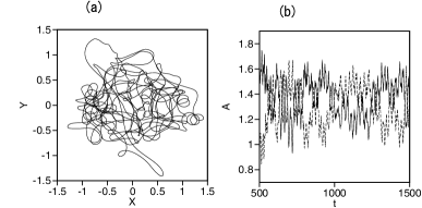
Figure 11: (a) The trajectory of chaotic motion of the center of mass of the semi-vortex soliton under the action of a shallow isotropic HO trapping potential, with $\Omega_{x}=\Omega_{y}=0.01$, other parameters being $d=0.02$, $\gamma=1$, $\lambda=1$. (b) The evolution of amplitudes of components $|\phi_{+}\left(x,y\right)|$ and $\left|\phi_{-}\left(x,y\right)\right|$ (solid and dashed curves, respectively) in the same case.

III Flipping-shuttle dynamics of two-dimensional SV (semi-vortex) solitons

The 2D GPE system, which includes the SOC of the Rashba type (again, with coefficient $\lambda$) and the RC terms in 2D, along with an harmonic-oscillator (HO) trapping potential (generally, an anisotropic one, with confining frequencies $\Omega_{x}\neq\Omega_{y}$), is written as a straightforward extension of the model considered in Ref. Sakaguchi :

$$i\frac{\partial\phi_{+}}{\partial t} = -\frac{1}{2}\nabla^{2}\phi_{+}-(|\phi_{+}|^{2}+\gamma|\phi_{-}|^{2})\phi_{+}+\lambda\left(\frac{\partial\phi_{-}}{\partial x}-i\frac{\partial\phi_{-}}{\partial y}\right)+\frac{1}{2}\left(\Omega_{x}^{2}x^{2}+\Omega_{y}^{2}y^{2}\right)\phi_{+}-d\phi_{-},$$

$$i\frac{\partial\phi_{-}}{\partial t} = -\frac{1}{2}\nabla^{2}\phi_{-}-(|\phi_{-}|^{2}+\gamma|\phi_{+}|^{2})\phi_{-}-\lambda\left(\frac{\partial\phi_{+}}{\partial x}+i\frac{\partial\phi_{+}}{\partial y}\right)+\frac{1}{2}\left(\Omega_{x}^{2}x^{2}+\Omega_{y}^{2}y^{2}\right)\phi_{-}-d\phi_{+}.$$ (20)

At $d=0$ and $\gamma\leq 1$, Eqs. (20) in free space (with $\Omega_{x,y}=0$) give rise to stable bright solitons in the form of the SVs, composed of an isotropic wave field with zero vorticity in one component, and a solitary vortex in the other. Loosely speaking, the SVs may be considered as the 2D generalization of the 1D striped solitons (in particular, the difference of even and odd parities of the two components of the 1D solitons resembles the difference of the zero and nonzero vorticities of the SV’s components). Note that, although coordinates $x$ and $y$ in the free-space version of Eq. (20) appear differently, the equations are invariant with respect to a change of the notation which readily swaps $x$ and $y$: $\tilde{\phi}_{+}\equiv\phi_{+}$, $\tilde{\phi}_{-}\equiv i\phi_{-}$, $\tilde{x}\equiv-y$, $\tilde{y}\equiv x$. The total norm of the 2D soliton is

$$N=\int\int\left[|\phi_{+}\left(x,y\right)|^{2}+\left|\phi_{-}\left(x,y\right)\right|^{2}\right]dxdy.$$ (21)

Similar to the 1D system, we here focus on the Manakov’s nonlinearity, with $\gamma=1$, which is quite close to the physically relevant situation, as mentioned above. First of all, in the free space ($\Omega_{x,y}=0$), results reported in Ref. Sakaguchi actually demonstrate that, under the action of the RC terms with strength $d$, the SV moves at a constant velocity,

$$v_{y}=d/\lambda.$$ (22)

Indeed, the transformation of Eq. (20) with $d=0$ and $\Omega_{x,y}=0$ into a reference frame moving in the $y$ direction with velocity $v_{y}$, which is carried out by means of the substitution,

$$\phi_{\pm}(x,y;t)=\tilde{\phi}_{\pm}\left(x,y-v_{y}t;t\right)\exp\left[iv_{y}y-\left(i/2\right)v_{y}^{2}t\right],$$ (23)

generates effective RC terms with $\tilde{d}=-\lambda v_{y}$ , which compensate the RC terms in Eq. (LABEL:1DSOC), thus making the existence of the solitons moving at velocity (22) obvious. In exact accordance with this, simulations of Eq. (20) with $\Omega_{x.y}=0$ produce stable SVs moving at a constant velocity in the $y$ direction, as shown in Fig. 6. The initial condition is taken not as Eq. (23) at $t=0$, but as the stationary SV state of Eq. (20) with $\Omega_{x,y}=0$ and without the RC term. The center of mass of the 2D solitons is defined as

$$\left\{X,Y\right\}=N^{-1}\int\int\left\{x,y\right\}(|\phi_{+}|^{2}+|\phi_{-}|^{2})dxdy$$ (24)

[cf. Eq. (19) in the 1D model], where $N$ is the 2D norm defined as per Eq. (21). The numerically found velocity, $v_{y}\equiv dY/dt=0.05$, corresponding to the situation displayed in Fig. 6, precisely agrees with the value given by Eq. (22). Note that the same argument is not valid for the 1D system (LABEL:1DSOC), as the application of the transformation similar to that defined by Eq. (23) to system (LABEL:1DSOC) does not generate the RC terms.

Similar to the flipping oscillations between the even and odd components of 1D stripe solitons, in 2D the RC may cause periodic flippings between the SV with vorticities $\left(0,+1\right)$ in its components $\left(\phi_{+},\phi_{-}\right)$, and its mirror-image counterpart, with the vorticity set $\left(-1,0\right)$, provided that free motion in the $y$ direction (see Fig. 6) is arrested by the confining HO potential in Eq. (20) with $\Omega_{y}$ large enough, while $\Omega_{x}=0$ may be set, the confinement in the $x$ direction being unnecessary, as suggested by the results for the 1D system presented above. The initial condition for the direct numerical simulation of Eq. (20) is the stationary ground state of Eq. (20) with $d=0$, which includes the HO potential with $\Omega_{y}=1$ . A typical example of robust periodic flippings, coupled to the shuttle motion of the SV as a whole, is presented in Fig. 7. Further, Fig. 8 shows a cycle of the transformations of the fundamental (zero-vorticity) component into a vortex and back. The vortex enters the fundamental component ($\phi_{+}$) from the edge at the moment of time close to $t=61.5$, attains the central position at $t=123$, and then moves backwards, leaving the pattern through the same edge from which it has entered at $t=184.5$, when $\phi_{+}$ recurs to the zero-vorticity shape. The shuttle motion coupled to the intrinsic flippings is synchronized with them: the soliton reaches the leftmost position of $X\simeq 2$ at $t=123$, and returns to the center, $X=0$, at $t=246$.

Figure 9(a) shows, on the log-log scale, the dependence of the evolution period on the RC strength, $T(d)$, for $\lambda=1$ and $\gamma=1$, which is found to be $T\sim 1/\sqrt{d}$. This dependence is essentially the same as in the 1D system, cf. 2 (c), and the same qualitative explanation for it, which was presented above for the 1D case, applies in the present case as well. Figure 9(b) shows, on the log-log scale, the respective dependence $2\Xi(\lambda)$ at $d=0.01$ and $\gamma=1$. The dashed line is a line of $2\Xi=1.95/\lambda^{0.8}$.

Similar to the 1D system considered above, the analysis of the 2D model in the “under-Manakov” case, with $\gamma<1$, demonstrates that the flipping oscillations do not occur at too small values of the RC strength, $d$. In particular, Fig. 10(a) shows that stable flippings take place at $d=0.1$, while other parameters are fixed as $\lambda=1$, $\gamma=0$, and $N=4$, but the flipping regime does not occur in Fig. 10(b) at $d$ reduced to $0.05$, when the amplitudes of the two components oscillate without crossing zero. In this case, the critical value at which the flipping regime sets in is $d_{c}\approx 0.08$, cf. Fig. 4(c) in the 1D case.

Lastly, it is relevant to stress that the presence of the anisotropic HO trapping potential, which acts only along the $y$ direction in the case corresponding to Figs. 7 and 9, is essential for supporting the robust flipping-shuttle dynamical regime for the SVs in the 2D geometry. If an isotropic HO trapping potential is used, with $\Omega_{x}=\Omega_{y}$, the evolution of the SV becomes chaotic under the action of the RC, and regular shuttle motion is not observed, as shown in Fig. 11. A possible explanation to this may be the mismatch between the isotropic shape of the trapping potential and anisotropic structure of the SOC operator in Eq. (20). In a detailed form, this situation may be analyzed in a finite-mode approximation, expanding the two components of the wave function over a truncated set of eigenstates of the isotropic HO Hamiltonian, and, accordingly, replacing the coupled GPEs by a system of ordinary differential equations for the evolution of amplitudes of the truncated expansion (cf. Ref. Driben ), but detailed analysis of this approach is beyond the scope of the present work.

IV Conclusion

The objective of this work is to expand the variety of macroscopic quantum effects produced by coherent evolution of matter waves in BEC. To this end, we have considered the dynamics of 1D and 2D solitons in the binary SOC (spin-orbit-coupled) system with intrinsic self- and cross-attractive interactions, under the action of the linear RC (Rabi coupling). The latter ingredient of the system can be readily induced by a resonant GHz-frequency electromagnetic wave mixing different atomic states representing the two components of the binary condensate. The RC gives rise to periodic flippings between the spatially even and odd components of 1D striped solitons, and between the zero-vorticity and vortical components of the stable 2D semi-vortices, in the presence of a quasi-1D confining potential. In both cases, the intrinsic oscillations of the internal structure of the soliton are coupled to the periodic shuttle motion of the soliton as a whole. These results predict a possibility to observe new macroscopic manifestations of the SOC in the matter-wave dynamics.

As an extension of the present analysis, it may be relevant to consider interactions, including collisions, between 1D and 2D solitons performing the flipping-shuttle oscillations. A challenging possibility is to extend the consideration to the full 3D setting.

References

- (1) L. Pitaevskii and S. Stringari, Bose-Einstein Condensation (Oxford University Press: Oxford, UK, 2003).
- (2) I. Bloch, J. Dalibard, and W. Zwerge, Many-body physics with ultracold gases, Rev. Mod. Phys. 80, 885-964 (2008).
- (3) R. Carretero-González, D. J. Frantzeskakis, and P. G. Kevrekidis, Nonlinear waves in Bose–Einstein condensates: physical relevance and mathematical techniques, Nonlinearity 21, R139-R202 (2008).
- (4) P. Hauke, F. M. Cucchietti, L. Tagliacozzo, I. Deutsch, and M. Lewenstein, Can one trust quantum simulators?, Rep. Prog. Phys. 75, 082401 (2012).
- (5) Y. J. Lin, K. Jimenez-Garcia, and I. B. Spielman, Spin-orbit coupled Bose - Einstein condensates, Nature 471, 83-86 (2011).
- (6) J. -Y. Zhang, S. -C. Ji, Z. Chen, L. Zhang, Z. -D. Du, B. Yan, G. -S. Pan, B. Zhao, Y. -J. Deng, H. Zhai, S. Chen, and J. -W. Pan, Collective dipole oscillations of a spin-orbit coupled Bose-Einstein condensate, Phys. Rev. Lett. 109, 115301 (2012).
- (7) D. L. Campbell, G. Juzeliūnas, and I. B. Spielman, Realistic Rashba and Dresselhaus spin-orbit coupling for neutral atoms, Phys. Rev. A 84, 025602 (2011).
- (8) Y. A. Bychkov and E. I. Rashba, Oscillatory effects and the magnetic susceptibility of carriers in inversion layers, J. Phys. C 17, 6039-6045 (1984).
- (9) G. Dresselhaus, Spin-orbit coupling effects in zinc blende structures, Phys. Rev 100, 580-586 (1955).
- (10) V. Galitski and I. B. Spielman, Spin-orbit coupling in quantum gases, Nature 494, 49-54 (2013).
- (11) H. Zhai, Degenerate quantum gases with spin–orbit coupling: a review, Rep. Prog. Phys. 78, 026001 (2015).
- (12) Z. Wu, L. Zhang, W. Sun, X. T. Xu, B. Z. Wang, S. C. Ji, Y. Deng, S. Chen, X. J. Liu, and J. W. Pan, Realization of two-dimensional spin-orbit coupling for Bose - Einstein condensates, Science 354, 83-88 (2016).
- (13) A. L. Fetter, Rotating trapped Bose-Einstein condensates. Rev. Mod. Phys. 81, 647-691 (2009).
- (14) T. Kawakami, T. Mizushima, and K. Machida,Textures of spinor Bose - Einstein condensates with spin-orbit coupling, Phys. Rev. A 84, 011607 (2011).
- (15) B. Ramachandhran, B. Opanchuk, X. J. Liu, H. Pu, P. D. Drummond, and H. Hu, Half - quantum vortex state in a spin-orbit-coupled Bose - Einstein condensate, Phys. Rev. A 85, 023606 (2012).
- (16) H. Sakaguchi and B. Li, Vortex lattice solutions to the Gross-Pitaevskii equation with spin-orbit coupling in optical lattices. Phys. Rev. A 87, 015602 (2013).
- (17) W. Han, X. F. Zhang, S. W. Song, H. Saito, W. Zhang, W. M. Liu, and S. G. Zhang, Double-quantum spin vortices in spin-orbit-coupled Bose gases, Phys. Rev. A 94, 033629 (2016).
- (18) G. J., Conduit,Line of Dirac monopoles embedded in a Bose-Einstein condensate. Phys. Rev. A 86, 021605 (2012).
- (19) C. J. Wu, I. Mondragon-Shem, and X. F. Zhou, Unconventional Bose-Einstein condensations from spin-orbit coupling, Chin. Phys. Lett. 28, 097102 (2011).
- (20) T. Kawakami, T. Mizushima, M. Nitta, and K. Machida, Stable skyrmions in gauged Bose - Einstein condensates, Phys. Rev. Lett. 109, 015301 (2012).
- (21) V. Achilleos, J. Stockhofe, P. G. Kevrekidis, D. J. Frantzeskakis and P. Schmelcher, Matter-wave dark solitons and their excitation spectra in spin-orbit coupled Bose-Einstein condensates, EPL 103, 20002 (2013).
- (22) V. Achilleos, D. J. Frantzeskakis, and P. G. Kevrekidis, Beating dark-dark solitons and Zitterbewegung in spin-orbit-coupled Bose-Einstein condensates, Phys. Rev. A 89, 033636 (2014)
- (23) Y. V. Kartashov, V. V. Konotop, and F. Kh. Abdullaev, Gap solitons in a spin-orbit-coupled Bose-Einstein condensate, Phys. Rev. Lett. 111, 060402 (2013).
- (24) V. E. Lobanov, Y. V. Kartashov, and V. V. Konotop, Fundamental, multipole, and half-vortex gap solitons in spin-orbit coupled Bose-Einstein condensates. Phys. Rev. Lett. 112, 180403 (2014).
- (25) O. Fialko, J. Brand, and U. Zülicke, Soliton magnetization dynamics in spin-orbit-coupled Bose-Einstein condensates, Phys. Rev. A 85, 051605(R) (2012).
- (26) S. L. Cornish, N. R. Claussen, J. L. Roberts, E. A. Cornell, and C. E. Wieman,Stable 85Rb Bose-Einstein condensates with widely tunable interactions, Phys. Rev. Lett. 85, 1795-1795 (2000).
- (27) C. Chin, R. Grimm, P. Julienne, and E. Tiesinga, Feshbach resonances in ultracold gases, Rev. Mod. Phys. 82, 1225-1286 (2010).
- (28) K. E. Strecker, K. E., G. B. Partridge, A. G. Truscott, and R. G. Hulet, Formation and propagation of matter-wave soliton trains, Nature 417, 150-153 (2002).
- (29) L. Khaykovich, F. Schreck, G. Ferrari, T. Bourdel, J. Cubizolles, L. D. Carr, Y. Castin, and C. Salomon, Formation of a matter-wave bright soliton, Science 296, 1290-1293 (2002).
- (30) S. L. Cornish, S. T. Thompson, and C. E. Wieman, Formation of bright matter-wave solitons during the collapse of attractive Bose-Einstein condensates, Phys. Rev. Lett. 96, 170401 (2006).
- (31) A. L. Marchant, T. P. Billam, T. P. Wiles, M. M. H. Yu, S. A. Gardiner, and S. L. Cornish, Controlled formation and reflection of a bright solitary matter-wave, Nature Comm. 4, 1865 (2013).
- (32) S. Burger, K. Bongs, S. Dettmer, W. Ertmer, K. Sengstock, A. Sanpera, G. V. Shlyapnikov, and M. Lewenstein, Dark solitons in Bose-Einstein condensates, Phys. Rev. Lett. 83, 5198-5201 (1999).
- (33) I. A. Bhat, T. Mithun, B. A. Malomed, and K. Porsezian, Modulational instability in binary spin-orbit-coupled Bose-Einstein condensates, Phys. Rev. A 92, 063606 (2015).
- (34) Y. Xu, Y. Zhang, and B. Wu, Bright solitons in spin-orbit-coupled Bose-Einstein condensates, Phys. Rev. A 87, 013614 (2013).
- (35) L. Salasnich and B. A. Malomed, Localized modes in dense repulsive and attractive Bose-Einstein condensates with spin-orbit and Rabi couplings, Phys. Rev. A 87, 063625 (2013).
- (36) V. Achilleos, D. J. Frantzeskakis, P. G. Kevrekidis, and D. E. Pelinovsky, Matter-wave bright solitons in spin-orbit coupled Bose-Einstein condensates, Phys. Rev. Lett. 110, 264101 (2013).
- (37) Y.-K. Liu and S.-J. Yang, Exact solitons and manifold mixing dynamics in the spin-orbit–coupled spinor condensates, EPL 108, 30004 (2014).
- (38) Y. V. Kartashov, V. V. Konotop, and D. A. Zezyulin, Bose-Einstein condensates with localized spin-orbit coupling: Soliton complexes and spinor dynamics, Phys. Rev. A 90, 063621 (2014).
- (39) S. Peotta, F. Mireles, and M. Di Ventra, Edge binding of sine-Gordon solitons in spin-orbit-coupled Bose-Einstein condensates, Phys. Rev. A 91, 021601(R) (2015).
- (40) P. Beličev, G. Gligorić, J. Petrović, A. Maluckov, L. Hadžievski, and B. Malomed, Composite localized modes in discretized spin-orbit-coupled Bose-Einstein condensates, J. Phys. B At. Mol. Opt. Phys. 48, 065301 (2015).
- (41) S. Gautam and S. K. Adhikari, Mobile vector soliton in a spin-orbit coupled spin-1 condensate, Laser Phys. 12, 045501 (2015).
- (42) S. Gautam and S. K. Adhikari, Vector solitons in a spin-orbit-coupled spin-2 Bose-Einstein condensate, Phys. Rev. A 91, 063617 (2015).
- (43) L. Wen, Q. Sun, Y. Chen, D.-S. Wang, J. Hu, H. Chen, W.-M. Liu, G. Juzeliūnas, B. A. Malomed, and A.-C. Ji, Motion of solitons in one-dimensional spin-orbit-coupled Bose-Einstein condensates, Phys. Rev. A 94, 061602(R) (2016).
- (44) X. Zhu, H. Li, Z. Shi, Y. Xiang, and Y. He, Gap solitons in spin-orbit-coupled Bose-Einstein condensates in mixed linear-nonlinear optical lattices, J. Phys. B: At. Mol. Opt. Phys. 50, 155004 (2017).
- (45) G. Fibich, The Nonlinear Schrödinger equation: Singular Solutions and Optical Collapse (Springer: Cham, Heidelberg, New York, Dordrecht, London, 2015).
- (46) H. Sakaguchi, B. Li, B. A. Malomed, Phys. Rev. E 89, 032920 (2014).
- (47) L. Salasnich, W. B. Cardoso, and B. A. Malomed, Localized modes in quasi-two-dimensional Bose-Einstein condensates with spin-orbit and Rabi couplings, Phys. Rev. A 90, 033629 (2014).
- (48) H. Sakaguchi and B. A. Malomed, Discrete and continuum composite solitons in Bose-Einstein condensates with the Rashba spin-orbit coupling in one and two dimensions, Phys. Rev. E 90, 062922 (2014).
- (49) Y. V. Kartashov, B. A. Malomed, V. V. Konotop, V. E. Lobanov, and L. Torner, Stabilization of solitons in bulk Kerr media by dispersive coupling, Opt. Lett. 40, 1045-1048 (2015).
- (50) H. Sakaguchi and B. A. Malomed, One- and two-dimensional solitons in -symmetric systems emulating spin-orbit coupling, New J. Phys. 18, 105005 (2016).
- (51) I. A. Shelykh, A. V. Kavokin, Y. G. Rubo, T. C. H. Liew, and G. Malpuech, Polariton polarization-sensitive phenomena in planar semiconductor microcavities, Semicond. Sci. Technol. 25, 013001 (2010); V. G. Sala, D. D. Solnyshkov, I. Carusotto, T. Jacqmin, A. Lemaître, H. Terças, A. Nalitov, M. Abbarchi, E. Galopin, I. Sagnes, J. Bloch, G. Malpuech, and A. Amo, Spin-orbit coupling for photons and polaritons in microstructures, Phys. Rev. X 5, 011034 (2015).
- (52) K. Y. Bliokh, F. J. Rodríguez-Fortuño, F. Nori, and A. V. Zayats, Spin-orbit interactions of light, Nature Photonics 9, 796-808 (2016).
- (53) H. Sakaguchi, B. A. Malomed, and D. V. Skryabin, Spin-orbit coupling and nonlinear modes of the polariton condensate in a harmonic trap, New J. Phys. 19, 08503 (2017).
- (54) H. Sakaguchi, E. Ya. Sherman, and B. A. Malomed, Vortex solitons in two-dimensional spin-orbit coupled Bose-Einstein condensates: Effects of the Rashba-Dresselhaus coupling and the Zeeman splitting, Phys. Rev. E 94, 032202 (2016).
- (55) B. A. Malomed, Polarization dynamics and interactions of solitons in a birefringent optical fiber, Phys. Rev. A 43, 410-423 (1991).
- (56) S. V. Manakov, Theory of 2-dimensional stationary self-focusing of electromagnetic waves, Zh. Eksp. Teor. Fiz. 65, 505-516 (1973) [Sov. Phys. JETP 38, 24S (1974)].
- (57) Y. Zhang, Y. Xu, and T. Busch, Gap solitons in spin-orbit-coupled Bose-Einstein condensates in optical lattices, Phys. Rev. A 91, 043629 (2015).
- (58) Y.-C. Zhang, Z.-W. Zhou, B. A. Malomed, and H. Pu, Stable solitons in three dimensional free space without the ground state: Self-trapped Bose-Einstein condensates with spin-orbit coupling, Phys. Rev. Lett. 115, 253902 (2015).
- (59) L. Calderaro, A. L. Fetter, P. Massignan, and P. Wittek, Vortex dynamics in coherently coupled Bose-Einstein condensates, Phys. Rev. A 95, 023605 (2017).
- (60) R. J. Ballagh, K. Burnett, and T. F. Scott, Theory of an output coupler for Bose-Einstein condensed atoms, Phys. Rev. Lett. 78, 1607-1611 (1997).
- (61) J. Williams, R. Walser, J. Cooper, E. Cornell, and M. Holland, Nonlinear Josephson-type oscillations of a driven, two-component Bose-Einstein condensate, Phys. Rev. A 59, R31-R34 (1999).
- (62) P. Öhberg and S. Stenholm, Internal Josephson effect in trapped double condensates, Phys. Rev. A 59, 3890-3895 (1999).
- (63) D. T. Son and M. A. Stephanov, Domain walls of relative phase in two-component Bose-Einstein condensates, Phys. Rev. A 65, 063621 (2002).
- (64) S. D. Jenkins and T. A. B. Kennedy, Dynamic stability of dressed condensate mixtures, Phys. Rev. A 68, 053607 (2003).
- (65) T. L. Ho, Spinor Bose condensates in optical traps, Phys. Rev. Lett. 81, 742-745 (1998).
- (66) M. V. Tratnik and J. E. Sipe, Bound solitary waves in a birefringent optical fiber, Phys. Rev. A 38, 2011-2017 (1988).
- (67) S. Trillo, S. Wabnitz, W. C. Banyai, N. Finlayson, C. T. Seaton, G. I. Stegeman, and R. H. Stolen, Observation of ultrafast nonlinear polarization switching induced by polarization instability in a birefringent fiber rocking filter, IEEE J. Quant. Elect. 25, 104-112 (1989).
- (68) Y. Li, Y. Liu, Z. Fan, W. Pang, S. Fu, and B. A. Malomed, Two-dimensional dipolar gap solitons in free space with spin-orbit coupling, Phys. Rev. A 95, 063613 (2017).
- (69) R. Driben, V. V. Konotop, B. A. Malomed, and T. Meier, Dynamics of dipoles and vortices in nonlinearly coupled three-dimensional field oscillators, Phys. Rev. E 94, 012207 (2016).