Self-similar profiles for homoenergetic solutions of the Boltzmann equation: particle velocity distribution and entropy

Abstract

In this paper we study a class of solutions of the Boltzmann equation which have the form $f\left(x,v,t\right)=g\left(v-L\left(t\right)x,t\right)$ where $L\left(t\right)=A\left(I+tA\right)^{-1}$ with the matrix $A$ describing a shear flow or a dilatation or a combination of both. These solutions are known as homoenergetic solutions. We prove existence of homoenergetic solutions for a large class of initial data. For different choices for the matrix $A$ and for different homogeneities of the collision kernel, we characterize the long time asymptotics of the velocity distribution for the corresponding homoenergetic solutions. For a large class of choices of $A$ we then prove rigorously the existence of self-similar solutions of the Boltzmann equation. The latter are non Maxwellian distributions and describe far-from-equilibrium flows. For Maxwell molecules we obtain exact formulas for the $H$-function for some of these flows. These formulas show that in some cases, despite being very far from equilibrium, the relationship between density, temperature and entropy is exactly the same as in the equilibrium case. We make conjectures about the asymptotics of homoenergetic solutions that do not have self-similar profiles.

1 Introduction.

In this paper we study homoenergetic solutions of the Boltzmann equation. Our approach is motivated by an invariant manifold of solutions of the equations of classical molecular dynamics with certain symmetry properties ([10, 11]).

Briefly and formally, this manifold can be described as follows. Choose a matrix $A\in M_{3\times 3}\left(\mathbb{R}\right)$, let $e_{1},e_{2},e_{3}$ be linearly independent vectors in $\mathbb{R}^{3}$, and consider a time interval $[0,a)$ such that $\det(I+tA)>0$ for $t\in[0,a)$ with $a>0$. Consider any number of atoms labeled $1,\dots,M$ with positive masses $m_{1},\dots,m_{M}$ and any initial conditions

$${y}_{k}(0)={y}^{0}_{k},\quad\dot{y}_{k}(0)={v}^{0}_{k},\quad k=1,\dots,M.$$ (1.1)

Call these $M$ atoms the simulated atoms. The simulated atoms will be subject to the equations of molecular dynamics (to be stated presently) with the initial conditions (1.1), yielding solutions $y_{k}(t)\in\mathbb{R}^{3},\ 0\leq t<a,\ k=1,\dots,M$. In addition there will be non-simulated atoms with time-dependent positions $y_{\nu,k}(t)$, indexed by a triple of integers $\nu=(\nu_{1},\nu_{2},\nu_{3})\in\mathbb{Z}^{3},\ \nu\neq(0,0,0)$ and $k=1,\dots,M$. The nonsimulated atom $(\nu,k)$ will have mass $m_{k}$. The positions of the nonsimulated atoms will be given by the following explicit formulas based on the positions of the simulated atoms:

$$y_{\nu,k}(t)=y_{k}(t)+(I+tA)(\nu_{1}e_{1}+\nu_{2}e_{2}+\nu_{3}e_{3}),\quad\nu=(\nu_{1},\nu_{2},\nu_{3})\in\mathbb{Z}^{3},\ k=1,\dots,M.$$ (1.2)

For $k=1,\dots,M$ let $f_{k}:\cdots\mathbb{R}^{3}\times\mathbb{R}^{3}\times{\mathbb{R}^{3}}\cdots\to\mathbb{R}$ be the force on simulated atom $k$. Naturally, the force on simulated atom $k$ depends on the positions of all the atoms. This force is required to satisfy the standard conditions of frame-indifference and permutation invariance [10]. Formally, the equations of molecular dynamics for the simulated atoms are:

$$m_{k}\ddot{y}_{k} = f_{k}(\dots,y_{\nu_{1},1},\dots,y_{\nu_{1},M},\dots,y_{\nu_{2},1},\dots,y_{\nu_{2},M},\dots),$$ (1.3)

$${y}_{k}(0) = {y}^{0}_{k},\quad\dot{y}_{k}(0)={v}^{0}_{k},\quad k=1,\dots,M.$$

Note that these are ODEs in standard form for the motions of the simulated atoms since, for the nonsimulated atoms, we assume that the formulas (1.2) have been substituted into the right hand side of (1.3). It is shown in [10] and [11] that, even though the motions of the nonsimulated atoms are only given by formulas, the equations of molecular dynamics are exactly satisfied for each nonsimulated atom.

While this is stated formally here, if conditions are given on the $f_{k}$ such that the standard existence and uniqueness theorem holds for the initial value problem (1.1), (1.3), then the result holds rigorously. The proof is a simple consequence of frame-indifference and permutation invariance of atomic forces. The result can be rephrased as the existence of a certain family of time-dependent invariant manifolds of molecular dynamics.

These results on molecular dynamics have a simple interpretation in terms of the molecular density function of the kinetic theory. Consider a molecular dynamics simulation of the type described above. Consider a ball $B_{r}(x)$ of any radius $r$ centered at $x=(I+tA)(\nu_{1}e_{1}+\nu_{2}e_{2}+\nu_{3}e_{3})$, $(\nu_{1},\nu_{2},\nu_{3})\in\mathbb{Z}^{3}$. The ansatz (1.2) implies that, the velocities of all atoms in the ball $B_{r}(x)$ are completely determined by those in the ball $B_{r}(0)$. But the molecular density function $f(t,x,v)$ of the kinetic theory is supposed to describe the probability density of finding velocities in the small neighborhood of a point $x$ at time $t$. Thus, the ansatz associated to this observation about balls can be immediately written down based on (1.2) and its time-derivative. It is

$$f(t,x,v)=g(t,v-A(I+tA)^{-1}x).$$ (1.4)

(The emergence of the quantity $A(I+tA)^{-1}$ arises from conversion to the Eulerian form of the kinetic theory.)

Besides the reasons mentioned below, the study of these solutions is interesting from the general perspective of non-equilibrium statistical mechanics. Essentially, we show for broad classes of choices of $A$, there exist solutions of the Boltzmann equation satisfying (1.4). This means that, in a precise sense, this invariant manifold of molecular dynamics is inherited by the Boltzmann equation. This is true despite the fact that the Boltzmann equation is time irreversible, while molecular dynamics is time reversible. It is then particularly interesting to look at the form of the entropy (minus the $H$-function) in these cases. We give explicit relations satisfied by the entropy in some cases, that can be considered as derived constitutive relations. It would now be extremely interesting to study these relations in molecular dynamics. Besides the entropy, our results give new insight into the relation between atomic forces and nonequilibrium behavior.

An alternative viewpoint leading to the same result is presented in Section 2. That derivation is based on the viewpoint of equidispersive solutions, i.e., an ansatz of the form

$$f\left(t,x,v\right)=g\left(t,w\right)\text{ \ \ with }w=v-\xi\left(t,x\right).$$ (1.5)

Under mild conditions of smoothness, this ansatz is found to reduce the Boltzmann equation if and only if $\xi(t,x)=A(I+tA)^{-1}x$.

Formally, if $f$ is a solution of the Boltzmann equation (2.1) of the form (1.4) the function $g$ satisfies

$$\partial_{t}g-L\left(t\right)w\cdot\partial_{w}g=\mathbb{C}g\left(w\right)$$ (1.6)

where the collision operator $\mathbb{C}$ is defined as in (2.1). These solutions are called homoenergetic solutions and were introduced by Galkin [14] and Truesdell [27].

Homoenergetic solutions of the Boltzmann equation have been studied in [1], [2], [3], [6], [7], [8], [14], [15], [16], [18], [24], [25], [27], [28]. Details about the precise contents of these papers will be given later in the corresponding sections where similar results appears. To summarize this literature, we refer to interaction potentials of the form $V\left(x\right)=\frac{1}{\left|x\right|^{\nu-1}}$, which have homogeneity of the kernel $\gamma=\frac{\nu-5}{\nu-1}$. The case of Maxwell molecules corresponds to the case $\nu=5$, that is, homogeneity $\gamma=0$. In this case the moments $M_{j,k}$ associated to the function $g$ defined in (2.6) satisfy a system of linear equations. As in the original work of Galkin [14] and Truesdell [27], most previous work is concerned with the computation of the evolution of the moments $M_{j,k}=\int v_{j}v_{k}gdv$, as well as higher order moments, in the case in which the kernel $B$ in (2.1) has homogeneity $\gamma=0$. The evolution equation for the moments yields a huge amount of information about quantities like the typical deviation of the velocity and similar quantities ([4, 18, 28]).

Referring to these studies of the equations of the moments, Truesdell and Muncaster [28] say, “To what extent the exact solutions in the class here exhibited correspond to solutions of the Maxwell-Boltzmann equation is not yet established $\dots$ It is not clear whether [the moments] correspond to a molecular density”. In this paper, although we will use at several places the information provided by the moments, we will be mostly concerned with a detailed description of the distribution of velocities and other quantities such as the $H$-function that are not accessible from the moment equations.

The initial value problem associated to (1.6) has been considered by Cercignani [6] for a particular choice of $L(t)$. More precisely, Cercignani in [6] (see also [7]) considered homoenergetic affine flows for the Boltzmann equation in the case of simple shear (cf., Theorem 3.7, case 3.7) proving existence in $L^{1}$ of the distribution function for a large class of interaction potentials which include hard sphere and angular cut-off interactions. These solutions are in general not self-similar.

In this paper we first prove the existence of a large class of homoenergetic solutions and we study their long time asymptotics. Their behavior strongly depends on the homogeneity of the collision kernel $B$ and on the particular form of the hyperbolic terms, namely $L\left(t\right)w\cdot\partial_{w}g$. We find that, depending on the homogeneity of the kernel, we have different behaviors of the solutions of the Boltzmann equations for large times. Indeed, we prove the existence of self-similar profiles for Maxwell molecules, when the hyperbolic part of the equation and the collision term are of the same order of magnitude as $t\rightarrow\infty$. The resulting self-similar solutions are different from the Maxwellian distributions. Indeed, they reflect a nonequilibrium regime due to the balance between the hyperbolic part of the equation (which reflects effects like shear, dilatation) and the collision term.

The plan of the paper is the following. In Section 2 we describe the main properties of homoenergetic solutions of the Boltzmann equation. In Section 3 we characterize the long time asymptotics of $\xi\left(t,x\right)=L\left(t\right)x=\left(I+tA\right)^{-1}Ax$, restricting ourselves to the case in which $\det(I+tA)>0$ holds for all $t\geq 0$. In Section 4 we prove well posedness for homoenergetic flows, and we prove existence of self-similar homoenergetic solutions. In Section 5 we apply the general theory of Section 4 to various homoenergetic flows described in Section 3. In Section 6 we propose some conjectures on solutions which cannot described by self-similar profiles. These correspond to cases of $L(t)$ and homogeneity $\gamma$ such that the collision term and the hyperbolic term do not balance. Some of these conjectures were arrived at by careful study of the corresponding formal Hilbert expansion, which is presented in a forthcoming paper [19].

An important comment on the solutions discussed in this paper concerns the thermodynamic entropy. Indeed, as we point out in Section 7, there are many analogies with the corresponding formulas for the entropy for equilibrium distributions, in spite of the fact that the distributions obtained in this paper concern non-equilibrium situations. For example, if we identify the entropy density $s$ with minus the $H$-function, then our asymptotic formulas for self-similar solutions yield the identity

$$\frac{s}{\rho}=\log\frac{e^{3/2}}{\rho}+C_{G}.$$ (1.7)

But despite the fact that $s,\rho$ and $e$ can be rapidly changing functions of time for self-similar homoenergetic solutions, the relation between them is asymptotically the same as in the equilibrium case (Maxwellian distribution), except for one important fact. That is, the constant $C_{G}$ is not the same as the constant as in the equibrium case: $C_{G}<C_{M}$ where $C_{M}$ is the corresponding value for the Maxwellian distribution.

Another interesting consequence of our results is further insight into the possibility (discussed in [28]) that our solutions for simple shear exhibit non-zero heat flux despite having zero temperature gradient, in contradiction to most versions of continuum thermodynamics. A conjectured scenario under which this could occur is described in Section 5.1.2.

At the end of the paper we give a table which summarizes the rigorous results and conjectures (see Section 8) and in Section 9 we conclude with a discussion to clarify the state-of-the-art of the analysis of homoenergetic solutions for the Boltzmann equation and we give some further perspectives.

2 Homoenergetic solutions of the Boltzmann equation

The classical Boltzmann equation has the form

$$\partial_{t}f+v\partial_{x}f =\mathbb{C}f\left(v\right)\ \ ,\ \ f=f\left(t,x,v\right)$$

$$\mathbb{C}f\left(v\right) =\int_{\mathbb{R}^{3}}dv_{\ast}\int_{S^{2}}d\omega B\left(n\cdot\omega,\left|v-v_{\ast}\right|\right)\left[f^{\prime}f_{\ast}^{\prime}-f_{\ast}f\right],\$$ (2.1)

where $S^{2}$ is the unit sphere in $\mathbb{R}^{3}$ and $n=n\left(v,v_{\ast}\right)=\frac{\left(v-v_{\ast}\right)}{\left|v-v_{\ast}\right|}.$ Here $(v,v_{\ast})$ is a pair of velocities in incoming collision configuration (see Figure 1) and $(v^{\prime},v_{\ast}^{\prime})$ is the corresponding pair of outgoing velocities defined by the collision rule

$$v^{\prime} =v+\left(\left(v_{\ast}-v\right)\cdot\omega\right)\omega,$$ (2.2)

$$v_{\ast}^{\prime} =v_{\ast}-\left(\left(v_{\ast}-v\right)\cdot\omega\right)\omega.$$ (2.3)

The unit vector $\omega=\omega(v,V)$ bisects the angle between the incoming relative velocity $V=v_{\ast}-v$ and the outgoing relative velocity $V^{\prime}=v_{\ast}^{\prime}-v^{\prime}$ as specified in Figure 1. The collision kernel $B\left(n\cdot\omega,\left|v-v_{\ast}\right|\right)$ is proportional to the cross section for the scattering problem associated to the collision between two particles. We use the conventional notation in kinetic theory, $f=f\left(t,x,v\right),\ f_{\ast}=f\left(t,x,v_{\ast}\right),\ f^{\prime}=f\left(t,x,v^{\prime}\right),\ \ f_{\ast}^{\prime}=f\left(t,x,v_{\ast}^{\prime}\right)$.

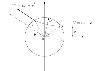
Figure 1: The two-body scattering. The solution of the two-body problem lies in a plane, which is taken to be the plane of the page, and the motion of molecule $\ast$ is plotted relative to the unstarred molecule. The scalar $\rho$ is the impact parameter expressed in microscopic units, $\rho\in[-1,1]$, and $\theta=\theta(\rho,|V|)$ is the scattering angle. The scattering vector of (2.2), (2.3) is the unit vector $\omega=\omega(v,V)$.

We will assume that the kernel $B$ is homogeneous with respect to the variable $\left|v-v_{\ast}\right|$ and we will denote its homogeneity by $\gamma,\$i.e.,

$$B\left(\frac{\left(v-v_{\ast}\right)\cdot\omega}{\left|v-v_{\ast}\right|},\lambda\left|v-v_{\ast}\right|\right)=\lambda^{\gamma}B\left(\frac{\left(v-v_{\ast}\right)\cdot\omega}{\left|v-v_{\ast}\right|},\left|v-v_{\ast}\right|\right),\ \ \lambda>0.$$ (2.4)

Given $f\left(t,x,v\right)$ we can compute the density $\rho$, the average velocity $V$ and the internal energy $\varepsilon$ at each point $x$ and time $t$ by means of

$$\rho\left(t,x\right)=\int_{\mathbb{R}^{3}}f\left(t,x,v\right)dv,\ \ \rho\left(t,x\right)V\left(t,x\right)=\int_{\mathbb{R}^{3}}f\left(t,x,v\right)vdv.$$ (2.5)

The internal energy $\varepsilon\left(t,x\right)$ (or temperature) is given by

$$\rho\left(t,x\right)\varepsilon\left(t,x\right)=\int_{\mathbb{R}^{3}}f\left(t,x,v\right)\left(v-V\left(t,x\right)\right)^{2}dv.$$

Homoenergetic solutions of (2.1) defined in [14] and [27] (cf., also [28]) are solutions of the Boltzmann equation having the form

$$f\left(t,x,v\right)=g\left(t,w\right)\text{ \ \ with }w=v-\xi\left(t,x\right).$$ (2.6)

Notice that, under suitable integrability conditions, every solution of (2.1) with the form (2.6) yields only time-dependent internal energy and density

$$\varepsilon\left(t,x\right)=\varepsilon\left(t\right)\ \ ,\ \ \rho\left(t,x\right)=\rho\left(t\right).$$ (2.7)

However, we have $V\left(t,x\right)=\xi\left(t,x\right)$ and therefore the average velocity depends also on the position.

A direct computation shows that in order to have solutions of (2.1) with the form (2.6) for a sufficiently large class of initial data we must have

$$\frac{\partial\xi_{k}}{\partial x_{j}}\text{ independent on }x\text{ and }\partial_{t}\xi+\xi\cdot\nabla\xi=0.$$ (2.8)

The first condition implies that $\xi$ is an affine function on $x$. However, we will restrict attention in this paper to the case in which $\xi$ is a linear function of $x,$ for simplicity, whence

$$\xi\left(t,x\right)=L\left(t\right)x,\$$ (2.9)

where $L\left(t\right)\in M_{3\times 3}\left(\mathbb{R}\right)$ is a $3\times 3$ real matrix. The second condition in (2.8) then implies that

$$\frac{dL\left(t\right)}{dt}+\left(L\left(t\right)\right)^{2}=0,\quad L(0)=A,$$ (2.10)

where we have added an initial condition.

Classical ODE theory shows that there is a unique continuous solution of (2.10),

$$L\left(t\right)=\left(I+tA\right)^{-1}A=A\left(I+tA\right)^{-1},\$$ (2.11)

defined on a maximal interval of existence $[0,a)$. On the interval $[0,a)$, $\det\left(I+tA\right)>0$.

3 Characterization of homoenergetic solutions defined for arbitrary large times.

In this section we describe the long time asymptotics of the function $\xi\left(t,x\right)=L\left(t\right)x=\left(I+tA\right)^{-1}Ax$ (cf. (2.9) and (2.11)). There are interesting choices of $A\in M_{3\times 3}\left(\mathbb{R}\right)$ for which $L\left(t\right)$ blows up in finite time, but we will restrict attention in this paper to the case in which the matrix $\det(I+tA)>0$ for all $t\geq 0$. We will use in the rest of the paper the following norm in $M_{3\times 3}\left(\mathbb{R}\right):$

$$\left\|M\right\|=\max_{i,j}\left\|m_{i,j}\right\|\ \ \text{with }M=\left(m_{i,j}\right)_{i,j=1,2,3}.$$ (3.1)

Theorem 3.1

Let $A\in M_{3\times 3}(\mathbb{R})$ satisfy $\det(I+tA)>0$ for $t\geq 0$ and let $L(t)=(I+tA)^{-1}A$. Assume $L$ does not vanish identically. Then, there is an orthonormal basis (possibly different in each case) such that the matrix of $L(t)$ in this basis has one of the following forms:

Case (i) Homogeneous dilatation:

$$L(t)=\frac{1}{t}I+O\bigg{(}\frac{1}{t^{2}}\bigg{)}\quad{\rm as}\ t\to\infty.$$ (3.2)

Case (ii) Cylindrical dilatation (K=0), or Case (iii) Cylindrical dilatation and shear ($K\neq 0$):

$$L(t)=\frac{1}{t}\left(\begin{array}[]{ccc}1&0&K\\ 0&1&0\\ 0&0&0\end{array}\right)+O\bigg{(}\frac{1}{t^{2}}\bigg{)}\quad{\rm as}\ t\to\infty.$$ (3.3)

Case (iv). Planar shear:

$$L(t)=\frac{1}{t}\left(\begin{array}[]{ccc}0&0&0\\ 0&0&K\\ 0&0&1\end{array}\right)+O\bigg{(}\frac{1}{t^{2}}\bigg{)}\quad{\rm as}\ t\to\infty.$$ (3.4)

Case (v). Simple shear:

$$L(t)=\left(\begin{array}[]{ccc}0&K&0\\ 0&0&0\\ 0&0&0\end{array}\right),\quad K\neq 0.$$ (3.5)

Case (vi). Simple shear with decaying planar dilatation/shear:

$$L(t)=\left(\begin{array}[]{ccc}0&K_{2}&0\\ 0&0&0\\ 0&0&0\end{array}\right)+\frac{1}{t}\left(\begin{array}[]{ccc}0&K_{1}K_{3}&K_{1}\\ 0&0&0\\ 0&K_{3}&1\end{array}\right)+O\bigg{(}\frac{1}{t^{2}}\bigg{)},\quad K_{2}\neq 0.$$ (3.6)

Case (vii). Combined orthogonal shear:

$$L(t)=\left(\begin{array}[]{ccc}0&K_{3}&K_{2}-tK_{1}K_{3}\\ 0&0&K_{1}\\ 0&0&0\end{array}\right),\quad K_{1}K_{3}\neq 0.$$ (3.7)

Proof of Theorem 3.7 The Jordan Canonical Form for real $3\times 3$ matrices says that there exists an orthonormal basis $e_{1},e_{2},e_{3}$ and a real invertible matrix $P$ such that $A=PJP^{-1}$, where the matrix $J$ has one of the following forms in this basis:

$$\left(\begin{array}[]{ccc}\alpha&\beta&0\\ -\beta&\alpha&0\\ 0&0&\gamma\end{array}\right),\left(\begin{array}[]{ccc}\lambda_{1}&0&0\\ 0&\lambda_{2}&0\\ 0&0&\lambda_{3}\end{array}\right),\left(\begin{array}[]{ccc}\xi&1&0\\ 0&\xi&0\\ 0&0&\eta\end{array}\right),\left(\begin{array}[]{ccc}\lambda&1&0\\ 0&\lambda&1\\ 0&0&\lambda\end{array}\right).$$ (3.8)

All entries are real and $\beta\neq 0$. In these four cases, respectively, we have that $\det(I+tA)$ is

$$((1+\alpha t)^{2}+t^{2}\beta^{2})(1+t\gamma),\quad(1+t\lambda_{1})(1+t\lambda_{2})(1+t\lambda_{3}),\quad(1+t\eta)(1+t\xi)^{2},\quad(1+t\lambda)^{3}$$ (3.9)

Therefore, necessary and sufficient conditions that $\det(I+tA)>0$ for $t\geq 0$ are, respectively,

$$\gamma\geq 0,\quad\quad\lambda_{1}\geq 0,\lambda_{2}\geq 0,\lambda_{3}\geq 0,\quad\quad\eta\geq 0,\xi\geq 0,\quad\quad\lambda\geq 0.$$ (3.10)

Again in this basis, we have that $L(t)=P(I+tJ)^{-1}JP^{-1}$ where, respectively,

$$(I+tJ)^{-1}J = \left(\begin{array}[]{ccc}\frac{\alpha+t(\alpha^{2}+\beta^{2})}{(1+t\alpha)^{2}+t^{2}\beta^{2}}&\frac{\beta}{(1+t\alpha)^{2}+t^{2}\beta^{2}}&0\\ \frac{-\beta}{(1+t\alpha)^{2}+t^{2}\beta^{2}}&\frac{\alpha+t(\alpha^{2}+\beta^{2})}{(1+t\alpha)^{2}+t^{2}\beta^{2}}&0\\ 0&0&\frac{\gamma}{1+t\gamma}\end{array}\right),\left(\begin{array}[]{ccc}\frac{\lambda_{1}}{1+t\lambda_{1}}&0&0\\ 0&\frac{\lambda_{2}}{1+t\lambda_{2}}&0\\ 0&0&\frac{\lambda_{3}}{1+t\lambda_{3}}\end{array}\right),$$ (3.24)

$$\left(\begin{array}[]{ccc}\frac{\xi}{1+t\xi}&\frac{1}{(1+t\xi)^{2}}&0\\ 0&\frac{\xi}{1+t\xi}&0\\ 0&0&\frac{\eta}{1+t\eta}\end{array}\right),\left(\begin{array}[]{ccc}\frac{\lambda}{1+t\lambda}&\frac{1}{(1+t\lambda)^{2}}&\frac{-t}{(1+t\lambda)^{3}}\\ 0&\frac{\lambda}{1+t\lambda}&\frac{1}{(1+t\lambda)^{2}}\\ 0&0&\frac{\lambda}{1+t\lambda}\end{array}\right)$$

The first matrix in (3.24) with $\gamma>0$ gives (3.2), and with $\gamma=0$ gives (3.3). To see the latter, note first that

$$\lim_{t\to\infty}P\left(\begin{array}[]{ccc}\frac{t\alpha+t^{2}(\alpha^{2}+\beta^{2})}{(1+t\alpha)^{2}+t^{2}\beta^{2}}&\frac{t\beta}{(1+t\alpha)^{2}+t^{2}\beta^{2}}&0\\ \frac{-t\beta}{(1+t\alpha)^{2}+t^{2}\beta^{2}}&\frac{t\alpha+t^{2}(\alpha^{2}+\beta^{2})}{(1+t\alpha)^{2}+t^{2}\beta^{2}}&0\\ 0&0&0\end{array}\right)P^{-1}=P(e_{1}\otimes e_{1}+e_{2}\otimes e_{2})P^{-1}=I-Pe_{3}\otimes P^{-T}e_{3}.$$ (3.25)

Let $a=Pe_{3}$ and $n=P^{-T}e_{3}$, so that $a\cdot n=1$. Note that any $a$ and $n$ satisfying $a\cdot n=1$ are possible by choosing (the invertible) $P=a\otimes e_{3}+n_{1}^{\perp}\otimes e_{2}+n_{2}^{\perp}\otimes e_{2}$, where $n_{1}^{\perp},n_{2}^{\perp}$ are orthonormal and perpendicular to $n$. The required basis can be taken as the orthonormal basis $\hat{e}_{1},\hat{e}_{2},n/|n|$ where $n\cdot\hat{e}_{2}=a\cdot\hat{e}_{2}=0$. In this basis $a=(-K/\nu,0,1/\nu)$ and $n=(0,0,\nu)$, $\nu\neq 0,K\in\mathbb{R}$, which gives (3.3).

Consider now the second matrix in (3.24). If $\lambda_{1}\lambda_{2}\lambda_{3}>0$ then we get the right hand expression in (3.2). If exactly one of $\lambda_{1},\lambda_{2},\lambda_{3}$ vanishes, say $\lambda_{3}=0$, we get the expression on the right of (3.25) multiplying $1/t$, and we recover case (3.3). If exactly two of $\lambda_{1},\lambda_{2},\lambda_{3}$ vanish, say $\lambda_{1}=\lambda_{2}=0$, then

$$\lim_{t\to\infty}P\left(\begin{array}[]{ccc}0&0&0\\ 0&0&0\\ 0&0&\frac{t\lambda_{3}}{1+t\lambda_{3}}\end{array}\right)P^{-1}=Pe_{3}\otimes e_{3}P^{-1}=Pe_{3}\otimes P^{-T}e_{3}.$$ (3.26)

As above, we write $a=Pe_{3},n=P^{-T}e_{3}$, so $a\cdot n=1$, and, as above, choose an orthonormal basis in which $a=(0,K\nu,\nu),n=(0,0,1/\nu)$, $K\in\mathbb{R},\nu\neq 0$. This gives (3.4).

Consider now the third matrix in (3.24). If $\xi=\eta=0$, we get immediately (3.5). If $\xi=0$ but $\eta\neq 0$, we have

$$P(I+tJ)^{-1}JP^{-1} = P\left(\begin{array}[]{ccc}0&1&0\\ 0&0&0\\ 0&0&0\end{array}\right)P^{-1}+\frac{1}{t}P\left(\begin{array}[]{ccc}0&0&0\\ 0&0&0\\ 0&0&\frac{t\eta}{1+t\eta}\end{array}\right)P^{-1}$$ (3.33)

$$= Pe_{1}\otimes P^{-T}e_{2}+\frac{1}{t}Pe_{3}\otimes P^{-T}e_{3}+O\bigg{(}\frac{1}{t^{2}}\bigg{)}.$$ (3.34)

Let $a=Pe_{1},n=P^{-T}e_{2},b=Pe_{3},m=P^{-T}e_{3}$. These are restricted by the necessary conditions

$$a\cdot n=0,\ b\cdot m=1,\ a\cdot m=0,\ b\cdot n=0,\ m\nparallel n,\ a\nparallel b.$$ (3.35)

Choose the orthonormal basis $\hat{e}_{1}=a/|a|,\hat{e}_{2}=n/|n|,\hat{e}_{3}=\hat{e}_{1}\times\hat{e}_{2}$. By scaling, we can assume without loss of generality that $a\cdot\hat{e}_{1}=1$ and $m\cdot\hat{e}_{3}=1$. In this basis $a=(1,0,0),n=(0,K_{2},0),b=(K_{1},0,1),m=(0,K_{3},1)$, $K_{2}\neq 0$. The conditions (3.35) are necessary and sufficient that the first two terms on the right hand side of (3.34) are $a\otimes n+(1/t)b\otimes m$, as can be verified by the choice $P=\hat{e}_{1}\otimes{e}_{1}+(1/K_{2})(\hat{e}_{2}-K_{3}\hat{e}_{3})\otimes{e}_{2}+(K_{1}\hat{e}_{1}+\hat{e}_{3})\otimes{e}_{3}$, which is invertible. The basis $\hat{e}_{1},\hat{e}_{2},\hat{e}_{3}$ is the required basis, and the result is given in (3.6).

Still considering the third matrix in (3.24), assume $\xi\neq 0$ and $\eta\neq 0$. We have

$$\lim_{t\to\infty}P\left(\begin{array}[]{ccc}\frac{t\xi}{1+t\xi}&\frac{t}{(1+t\xi)^{2}}&0\\ 0&\frac{t\xi}{1+t\xi}&0\\ 0&0&\frac{t\eta}{1+t\eta}\end{array}\right)=I,$$ (3.36)

and we recover case (3.2).

In cases (3.2)-(3.4) and (3.6) the error is clearly bounded by $const/t^{2}$.

Finally, consider the last matrix in (3.24). If $\lambda\neq 0$ we recover case (3.2). If $\lambda=0$, we have

$$P(I+tJ)^{-1}JP^{-1} = P\left(\begin{array}[]{ccc}0&1&-t\\ 0&0&1\\ 0&0&0\end{array}\right)P^{-1}$$ (3.40)

$$= Pe_{1}\otimes P^{-T}e_{2}+(Pe_{2}-tPe_{1})\otimes P^{-T}e_{3}.$$ (3.41)

Let $a=Pe_{1},n=P^{-T}e_{2},b=Pe_{2},m=P^{-T}e_{3}$. We have the necessary conditions

$$a\cdot n=0,\ b\cdot m=0,\ a\cdot m=0,\ b\cdot n=1,\ m\nparallel n,\ a\nparallel b.$$ (3.42)

Choose the basis $\hat{e}_{1}=a/|a|,\hat{e}_{3}=n/|n|,\hat{e}_{2}=\hat{e}_{3}\times\hat{e}_{1}$. By scaling, assume that $n\cdot\hat{e}_{2}=1$. In this basis $a=(K_{3},0,0),n=(0,1,K_{4}),b=(K_{5},1,0),m=(0,0,K_{1})$, $K_{1}K_{3}\neq 0$. The corresponding $P=K_{3}\hat{e}_{1}\otimes e_{1}+(K_{5}\hat{e}_{1}+\hat{e}_{2})\otimes e_{2}+(1/K_{1})(\hat{e}_{3}-K_{4}\hat{e}_{2})\otimes e_{3}$ is invertible. Putting $K_{2}=K_{3}K_{4}-K_{1}K_{5}$, we get case (3.7).

Remark 3.2

It is possible to obtain a more extensive classification of the homoenergetic flows if $\det(I+t^{*}A)=0$ at some $t^{*}>0$. In that case $L\left(t\right)$ blows-up at $t^{*}$ and the behavior of $L(t)$ can then be read off from (3.9), (3.24) in the proof of Theorem 3.7. Nevertheless, in this paper we will restrict our analysis only to the cases in which $L\left(t\right)$ is globally defined in time.

4 General properties of homoenergetic flows

4.1 Well posedness theory for homoenergetic flows of Maxwell molecules

We first prove using standard arguments for the Boltzmann equation that the homoenergetic flows with the form (2.6), (2.9), (2.10) exist for a large class of initial data $g_{0}\left(w\right).$ This question has been considered in [6], [7]. However, the approach used in those papers is based on the $L^{1}$ theory for Boltzmann equations (cf. [5]), and it will be more convenient for the type of arguments used in this paper to consider homoenergetic flows in the class of Radon measures. On the other hand, the analysis in [6], [7] is restricted to the case of simple shear (cf., (3.5)) and we will study more general classes of homoenergetic flows. Moreover, in some cases we will need to consider equations with additional terms which are due to rescalings of the solutions. For this reason we formulate here a well posedness theorem for a family of Boltzmann equations with the degree of generality that we will require. The class of equations that we will consider is the following one

$$\partial_{t}G-\partial_{w}\cdot\left(\left[Q(t)w\right]G\right) =\mathbb{C}G\left(w\right)$$ (4.1)

$$\mathbb{C}G\left(w\right) =\int_{\mathbb{R}^{3}}dw_{\ast}\int_{S^{2}}d\omega B\left(n\cdot\omega,\left|w-w_{\ast}\right|\right)\left[G^{\prime}G_{\ast}^{\prime}-G_{\ast}G\right]\ ,$$ (4.2)

$$G\left(0,w\right) =G_{0}\left(w\right),\$$ (4.3)

where

$$Q(\cdot)\in C^{1}\left(\left[0,\infty\right);M_{3\times 3}\left(\mathbb{R}\right)\right)\ \ ,\ \ \left\|Q(t)\right\|\leq c_{1}+c_{2}t,\text{ with }c_{1}>0,\ c_{2}>0.$$ (4.4)

with the norm $\left\|\cdot\right\|$ defined in (3.1). We will assume also in the following that the function

$$\Lambda\left(w,w_{\ast}\right)=\int_{S^{2}}B\left(n\cdot\omega,\left|w-w_{\ast}\right|\right)d\omega\ \ ,\ \ n=\frac{\left(w-w_{\ast}\right)}{\left|w-w_{\ast}\right|}$$ (4.5)

satisfies

$$\Lambda\text{ is continuous and}\ 0\leq\Lambda\left(w,w_{\ast}\right)\leq c_{3}\ \ \text{with }c_{3}>0.$$ (4.6)

We will prove well posedness results for the collision kernel associated to Maxwell molecules (or more generally Maxwell pseudomolecules in the notation of [28]). In this case, the kernel $B$ is homogeneous of degree zero in $\left|w-w_{\ast}\right|$ (e.g., the homogeneity parameter $\gamma=0$) and we then have $B\left(n\cdot\omega,\left|w-w_{\ast}\right|\right)=B\left(n\cdot\omega\right).$ This restriction to Maxwell molecules is the reason we assume the stringent boundedness condition (4.6).

We now introduce some definitions and notation. We denote by $\mathscr{M}_{+}\left(\mathbb{R}_{c}^{3}\right)$ the set of Radon measures in $\mathbb{R}_{c}^{3}$. We denote as $\mathbb{R}_{c}^{3}$ the compactification of $\mathbb{R}^{3}$ by means of a single point $\infty.$ This is a technical issue that we need in order to have convenient compactness properties for some subsets of $\mathscr{M}_{+}\left(\mathbb{R}_{c}^{3}\right).$ The space $C\left(\left[0,\infty\right):\mathscr{M}_{+}\left(\mathbb{R}_{c}^{3}\right)\right)$ is defined endowing $\mathscr{M}_{+}\left(\mathbb{R}_{c}^{3}\right)$ with the measure norm

$$\left\|\mu\right\|_{M}=\sup_{\varphi\in C\left(\mathbb{R}_{c}^{3}\right):\left\|\varphi\right\|_{\infty}=1}\left|\mu\left(\varphi\right)\right|=\int_{\mathbb{R}_{c}^{3}}\left|\mu\right|\left(dw\right).$$ (4.7)

We remark that this definition implies that the total measure of $\mathbb{R}_{c}^{3}$ is finite if $\mu\in\mathscr{M}_{+}\left(\mathbb{R}_{c}^{3}\right).$ Moreover $\varphi\in C\left(\mathbb{R}_{c}^{3}\right)$ implies that the limit value $\varphi\left(\infty\right)$ exists.

Given $G\in C\left(\left[0,\infty\right]:\mathscr{M}_{+}\left(\mathbb{R}_{c}^{3}\right)\right)$ we define

$$\mathbb{A}\left[G\right]\left(t,w\right)=\int_{\mathbb{R}^{3}}dw_{\ast}\int_{S^{2}}d\omega B\left(n\cdot\omega,\left|w-w_{\ast}\right|\right)G_{\ast}\left(t,\cdot\right).$$ (4.8)

Given $h_{0}\in\mathscr{M}_{+}\left(\mathbb{R}_{c}^{3}\right)$ we will denote as $S\left(t;t_{0}\right),\ t\geq t_{0}\geq 0,$ the operator $S_{G}\left(t;t_{0}\right):\mathscr{M}_{+}\left(\mathbb{R}_{c}^{3}\right)\rightarrow\mathscr{M}_{+}\left(\mathbb{R}_{c}^{3}\right)$ defined by means of

$$\partial_{t}h-\partial_{w}\cdot\left(\left[Q(t)w\right]h\right) =-\mathbb{A}\left[G\right]\left(t,w\right)h\ \ ,\ \ h\left(t_{0},\cdot\right)=h_{0}$$ (4.9)

$$h\left(t,w\right) =S_{G}\left(t;t_{0}\right)h_{0}.$$ (4.10)

The operator $S_{G}\left(t;t_{0}\right)$ is well defined, since (4.9) can be solved explicitly using the method of characteristics taking into account (4.4). The solution is given below in (4.22). A relevant point is that $\mathbb{A}\left[G\right]\left(w\right)\geq 0$ and as a consequence no divergences arise from large values of $\left|w\right|$. We will use the following concept of solutions of (4.1)-(4.3).

Definition 4.1

We will say that $G\in C\left(\left[0,\infty\right]:\mathscr{M}_{+}\left(\mathbb{R}_{c}^{3}\right)\right)$ is a mild solution of (4.1)-(4.3) with initial value $G\left(0,\cdot\right)=G_{0}\in\mathscr{M}_{+}\left(\mathbb{R}_{c}^{3}\right)$ if $G$ satisfies the following integral equation:

$$G\left(t,w\right)=S_{G}\left(t;0\right)G_{0}\left(w\right)+\int_{0}^{t}S_{G}\left(t;s\right)\mathbb{C}^{(+)}G\left(s,w\right)ds,$$ (4.11)

where the operator $S_{G}\left(t;s\right)$ is as in (4.10) and

$$\mathbb{C}^{\left(+\right)}G\left(w\right) =\int_{\mathbb{R}^{3}}dw_{\ast}\int_{S^{2}}d\omega B\left(n\cdot\omega,\left|w-w_{\ast}\right|\right)G^{\prime}G_{\ast}^{\prime},$$ (4.12)

$$\mathbb{C}^{\left(-\right)}G\left(w\right) =G\int_{\mathbb{R}^{3}}dw_{\ast}\int_{S^{2}}d\omega B\left(n\cdot\omega,\left|w-w_{\ast}\right|\right)G_{\ast}=\mathbb{A}\left[G\right]G.$$ (4.13)

We emphasize that (4.11) must be understood as an identity in the sense of measure, i.e., acting over an arbitrary test function $\varphi\in C\left(\mathbb{R}_{c}^{3}\right).$ Note also that all the operators appearing in (4.11) are well defined for $G\in C\left(\left[0,\infty\right]:\mathscr{M}_{+}\left(\mathbb{R}_{c}^{3}\right)\right)$ and that $S_{G}\left(t;s\right)$ is a bounded operator from $\mathscr{M}_{+}\left(\mathbb{R}_{c}^{3}\right)$ to $\mathscr{M}_{+}\left(\mathbb{R}_{c}^{3}\right)$ for $0\leq s\leq t\leq T<\infty.$

Theorem 4.2

Suppose that $G_{0}\in\mathscr{M}_{+}\left(\mathbb{R}^{3}\right)$ satisfies

$$\int_{\mathbb{R}^{3}}G_{0}\left(dw\right)<\infty,$$

Then, there exists a unique mild solution $G\in C\left(\left[0,\infty\right):\mathscr{M}_{+}\left(\mathbb{R}_{c}^{3}\right)\right)$ in the sense of Definition 4.1 to the initial value problem (4.1)-(4.3) with $Q$ and $B$ satisfying (4.4), (4.6). Moreover, the problem (4.1)-(4.3) is satisfied in the sense of measures.

Remark 4.3

Notice that since $B$ is continuous and it satisfies (4.6) we have that $\mathbb{C}^{\left(+\right)}G\left(w\right)$ and $\mathbb{C}^{\left(-\right)}G\left(w\right)$ in (4.12), (4.13) define measures in $\mathscr{M}_{+}\left(\mathbb{R}_{c}^{3}\right)$ and it makes sense to say that the equation (4.1)-(4.3) is satisfied in the sense of measures. The term $-\partial_{w}\cdot\left(\left[Q(t)w\right]G\right)$ is understood integrating by parts and passing the derivative to the test function $\varphi.$ The only difference between solutions in the sense of measures and the weak solutions defined in Definition 4.4 below is that in this second case we write the collision kernel in a symmetrized form which will be convenient in forthcoming computations.

We introduce now the concept of weak solution of (4.1)-(4.3) which will be also needed later.

Definition 4.4

We will say that $G\in C\left(\left[0,\infty\right):\mathscr{M}_{+}\left(\mathbb{R}_{c}^{3}\right)\right)$ is a weak solution of (4.1)-(4.3) with initial value $G\left(0,\cdot\right)=G_{0}\in\mathscr{M}_{+}\left(\mathbb{R}_{c}^{3}\right)$ if for any $T\in\left(0,\infty\right)$ and any test function $\varphi\in C\left(\left[0,T\right):C^{1}\left(\mathbb{R}_{c}^{3}\right)\right)$ the following identity holds

$$\int_{\mathbb{R}^{3}}\varphi\left(T,w\right)G\left(T,dw\right)-\int_{\mathbb{R}^{3}}\varphi\left(0,w\right)G_{0}\left(dw\right)$$ (4.14)

$$=-\int_{0}^{T}dt\int_{\mathbb{R}^{3}}\int\partial_{t}\varphi G\left(t,dw\right)-\int_{0}^{T}dt\int_{\mathbb{R}^{3}}\left[Q(t)w\cdot\partial_{w}\varphi\right]G\left(t,dw\right)$$

$$\quad+\frac{1}{2}\int_{0}^{T}dt\int_{\mathbb{R}^{3}}\int_{\mathbb{R}^{3}}\int_{S^{2}}d\omega G\left(t,dw\right)G\left(t,dw_{\ast}\right)B\left(n\cdot\omega,\left|w-w_{\ast}\right|\right)\Big{[}\varphi\left(t,w^{\prime}\right)+\varphi\left(t,w_{\ast}^{\prime}\right)\vspace{5mm}$$

$$\qquad-\varphi\left(t,w\right)-\varphi\left(t,w_{\ast}\right)\Big{]}.$$

We will use repeatedly the following norms:

$$\left\|G\right\|_{1,s}=\int_{\mathbb{R}^{3}}\left(1+\left|w\right|^{s}\right)G\left(dw\right)\ \ \text{for\ }G\in\mathscr{M}_{+}\left(\mathbb{R}_{c}^{3}\right)\text{\ },\ \ s>0$$ (4.15)

Theorem 4.5

Suppose that $G\in C\left(\left[0,\infty\right):\mathscr{M}_{+}\left(\mathbb{R}_{c}^{3}\right)\right)$ is a mild solution of (4.1)-(4.3) with $Q$ and $B$ satisfying (4.4), (4.6) and initial value $G\left(0,\cdot\right)=G_{0}\in\mathscr{M}_{+}\left(\mathbb{R}_{c}^{3}\right).$ Then $G$ is also a weak solution of (4.1)-(4.3) in the sense of Definition 4.2. Suppose that in addition $G_{0}$ satisfies

$$\left\|G_{0}\right\|_{1,s}<\infty$$ (4.16)

for some $s>0.$ Then the mild solution of (4.1)-(4.3) satisfies

$$\sup_{0\leq t\leq T}\left\|G\left(t,\cdot\right)\right\|_{1,s}<C\left(T,\left\|G_{0}\right\|_{M}\right)\left\|G_{0}\right\|_{1,s}<\infty$$ (4.17)

for any $T\in\left(0,\infty\right).$ Moreover, if $s>2$ the identity (4.14) is satisfied for any test function $\varphi\in C\left(\left[0,T\right]:C^{1}\left(\mathbb{R}_{c}^{3}\right)\right)$ such that $\left|\varphi\left(w\right)\right|+\left|w\right|\left|\nabla_{v}\varphi\left(w\right)\right|\leq C_{0}\left(1+\left|w\right|^{2}\right)$.

Proof of Theorem 4.2. Given $T\in\left(0,\infty\right),$ we define an operator $\mathscr{T}_{T}:C\left(\left[0,T\right]:\mathscr{M}_{+}\left(\mathbb{R}_{c}^{3}\right)\right)\rightarrow C\left(\left[0,T\right]:\mathscr{M}_{+}\left(\mathbb{R}_{c}^{3}\right)\right)$ by means of

$$\mathscr{T}_{T}\left[G\right]\left(t,w\right)=S_{G}\left(t;0\right)G_{0}\left(w\right)+\int_{0}^{t}S_{G}\left(t;s\right)\mathbb{C}^{(+)}G\left(s,w\right)ds,\ \ 0\leq t\leq T$$

where $S_{G}\left(t;s\right)$ is as in (4.10). Then, due to (4.11) the proof of the Theorem reduces to proving existence and uniqueness of solutions for the fixed point problem

$$G=\mathscr{T}_{T}\left[G\right].$$

We prove that the operator $\mathscr{T}_{T}$ is contractive if $T>0$ is sufficiently small. To this end we prove the following estimates:

$$\left\|\mathbb{C}^{(+)}G\right\|_{M} \leq C\left\|G\right\|_{M}^{2}$$ (4.18)

$$\left\|\mathbb{C}^{(+)}G_{1}-\mathbb{C}^{(+)}G_{2}\right\|_{M} \leq C\left(\left\|G_{1}\right\|_{M}+\left\|G_{2}\right\|_{M}\right)\left\|G_{1}-G_{2}\right\|_{M}$$ (4.19)

where the norm $\left\|\cdot\right\|_{M}$ is as in (4.7) and we have used (4.6) as well as the fact that the mapping $\left(w,w_{\ast}\right)\rightarrow\left(w^{\prime},w_{\ast}^{\prime}\right)$ is bijective and that the symplectic identity $dwdw_{\ast}=dw^{\prime}dw_{\ast}^{\prime}$ holds (cf., (2.2), (2.3)). We define $\mathscr{A}\subset C\left(\left[0,T\right]:\mathscr{M}_{+}\left(\mathbb{R}_{c}^{3}\right)\right)$ by

$$\mathscr{A}=\left\{G\in C\left(\left[0,T\right]:\mathscr{M}_{+}\left(\mathbb{R}_{c}^{3}\right)\right):\left\|G\left(\cdot,t\right)\right\|_{M}\leq 2\left\|G_{0}\right\|_{M}\text{ \ for }t\in\left[0,T\right]\right\}.$$

On the other hand we have the following estimates:

$$\left\|S_{G}\left(t;s\right)\right\|\leq 1\ \ \text{for }0\leq s\leq t<\infty,$$ (4.20)

where we denote the norm on the space $\mathscr{L}\left(\mathscr{M}_{+}\left(\mathbb{R}_{c}^{3}\right),\mathscr{M}_{+}\left(\mathbb{R}_{c}^{3}\right)\right)$ by $\left\|\cdot\right\|$. Moreover we have

$$\left\|S_{G_{1}}\left(t;s\right)-S_{G_{2}}\left(t;s\right)\right\|\leq CT\left\|G_{1}-G_{2}\right\|_{T},\ \text{ }0\leq s\leq t\leq T.$$ (4.21)

Here we used the norm $\left\|\cdot\right\|_{T}$ given by:

$$\left\|G\right\|_{T}=\sup_{t\in\left[0,T\right]}\left\|G\left(\cdot,t\right)\right\|_{M}.$$

The estimate (4.20) follows by integrating (4.9) and using $\mathbb{A}\left[G\right]\left(t,w\right)\geq 0.$ On the other hand, (4.21) can be proved using the representation formula for $S_{G}\left(t;s\right)$:

$$S_{G}\left(t;s\right)h_{0}\left(w\right)=\exp\left(-\int_{s}^{t}\mathbb{A}\left[G\right]\left(\xi,U\left(t,\xi\right)w\right)d\xi\right)\exp\left(\int_{s}^{t}\mathop{\rm tr}\left(Q\left(\xi\right)\right)d\xi\right)h_{0}\left(U\left(t;s\right)w\right)$$ (4.22)

where:

$$\frac{\partial\left[U\left(s;t\right)w\right]}{\partial t}=-Q(t)U\left(s;t\right)w\ \ ,\ \ U\left(s;s\right)w=w\in\mathbb{R}^{3}.$$

Then, (4.21) follows using that $\left|e^{-x_{1}}-e^{-x_{2}}\right|\leq\left|x_{1}-x_{2}\right|$, and $\sup_{w\in\mathbb{R}^{3}}\left|\mathbb{A}\left[G_{1}\right]\left(w\right)-\mathbb{A}\left[G_{2}\right]\left(w\right)\right|\leq C\left\|G_{1}-G_{2}\right\|_{M}$ yields the estimate

$$\left\|\left[S_{G_{1}}\left(t;s\right)-S_{G_{2}}\left(t;s\right)\right]h_{0}\right\|_{M}$$

$$\leq CT\left\|G_{1}-G_{2}\right\|_{T}\int_{\mathbb{R}^{3}}h_{0}\left(U\left(t,s\right)w\right)dw$$

$$\leq CT\left\|G_{1}-G_{2}\right\|_{T}\int_{\mathbb{R}^{3}}h_{0}\left(w\right)\mathop{\rm Jac}\left(U\left(s,t\right)\right)dw$$

$$\leq\tilde{C}T\left\|G_{1}-G_{2}\right\|_{T}\left\|h_{0}\right\|_{M}.$$

Combining (4.18), (4.19), (4.20), (4.21) we obtain that

$$\left\|\mathscr{T}_{T}\left[G\right]\right\|_{T}\leq\left\|G_{0}\right\|_{M}+4C\left\|G_{0}\right\|_{M}^{2}T$$ (4.23)

for any $G\in\mathscr{A}$. We have also

$$\left\|\mathscr{T}_{T}\left[G_{1}\right]-\mathscr{T}_{T}\left[G_{2}\right]\right\|_{T}\leq C\left\|G_{0}\right\|_{M}T\left\|G_{1}-G_{2}\right\|_{T}.$$

Therefore, the operator $\mathscr{T}_{T}\left[G\right]$ is contractive in the space $\mathscr{A}$ with a metric given by the norm $\left\|\cdot\right\|_{T}$ if $T$ is sufficiently small. This implies the existence of a mild solution in the time interval $\left[0,T\right]$ for $T$ sufficiently small. Notice that the fact that $G$ is nonnegative follows immediately due to the choice of the space of functions $\mathscr{A}$.

Applying the differential operator $\partial_{t}-\partial_{w}\cdot\left[Q(t)w\right]$ to (4.11) we obtain, using (4.9), (4.10) that the following identity holds in the sense of measures (i.e. the whole expression is understood using a test function $\varphi=\varphi\left(w\right)$):

$$\partial_{t}G\left(t,w\right)-\partial_{w}\cdot\left[Q(t)wG\left(t,w\right)\right]=\mathbb{C}^{(+)}G\left(t,w\right)-\mathbb{A}\left[G\right]\left(t,w\right)G\left(t,w\right)$$ (4.24)

whence $G$ satisfies (4.1)-(4.3) in the sense of measures. Integrating (4.24) we obtain

$$\left\|G\left(\cdot,t\right)\right\|_{M}=\left\|G_{0}\right\|_{M}\text{ \ for }0\leq t\leq T.$$ (4.25)

Therefore, using a similar argument we can extend the solution to an interval $\left[T,T+\delta\right]$ and iterating we then obtain a global solution defined for $0\leq t<\infty.$ Notice that the constants $C$ above depend on the time $T$ where we start the iteration argument due to the fact that $\left\|Q\left(t\right)\right\|$ can increase as $t\rightarrow\infty,$ but this norm is bounded for any finite interval $0\leq t\leq T$ and therefore we can prove global existence.  ∎

Proof of Theorem 4.5. Multiplying (4.24) by a test function $\varphi\left(t,w\right)$ integrating by parts and using a standard symmetrization argument on the right-hand side of (4.24) (cf. [9], [28]) and integrating in $t\in\left[0,T\right]$ we obtain (4.14).

We now prove that under the assumption (4.16) the solution obtained in Theorem 4.2 satisfies (4.17). Using the symplectic formula $dw^{\prime}dw_{\ast}^{\prime}=dwdw_{\ast}$ (cf. (2.2), (2.3)) and (4.12) we obtain

$$\left\|\mathbb{C}^{(+)}G\right\|_{1,s}\leq C\left\|G\right\|_{1,s}\left\|G\right\|_{M}\ \ ,\ \ G\in\mathscr{M}_{+}\left(\mathbb{R}_{c}^{3}\right).$$ (4.26)

where $s>0.$ On the other hand we claim that

$$\left\|S_{G}\left(t;s\right)G\right\|_{1,s}\leq C_{s}\left(T\right)\left\|G\right\|_{1,s}\ \ ,\ \ 0\leq s\leq t\leq T<\infty\ ,\ \ G\in\mathscr{M}_{+}\left(\mathbb{R}_{c}^{3}\right).$$ (4.27)

This estimate follows by multiplying (4.9) by the test functions $1$ and $\left|w\right|^{s},$ using that $\mathbb{A}\left[G\right]\left(t,w\right)\geq 0$, integrating over $\mathbb{R}^{3}$ and using a Gronwall-type argument. Then, estimating $\left\|G\left(t,\cdot\right)\right\|_{1,s}$ in (4.11) and using (4.26), (4.27) as well as the mass conservation property (4.25) we obtain

$$\left\|G\left(t,\cdot\right)\right\|_{1,s}\leq C_{s}\left(T\right)\left\|G_{0}\right\|_{1,s}+C_{s}\left(T\right)\left\|G_{0}\right\|_{M}\int_{0}^{t}\left\|G\left(s,\cdot\right)\right\|_{1,s}ds\ \ ,\ \ 0\leq t\leq T$$

whence (4.17) follows using Gronwall’s Lemma.

The fact that the identity (4.14) in Definition 4.4 is satisfied for test functions $\varphi$ bounded by a quadratic function as stated in the statement of Theorem 4.5 then follows by approximating the test function $\varphi$ by a sequence of test functions $\varphi_{n}\in C\left(\mathbb{R}_{c}^{3}\right)$ and using the fact that (4.17) implies that the contribution of the integrals due to the sets with $\left|w\right|\geq R$ tends to zero as $R\rightarrow\infty.$  ∎

Remark 4.6

Suppose that $G_{0}$ satisfies $\left\|G_{0}\right\|_{1,s}<\infty,$ and let $G$ be the corresponding solution of (4.1)-(4.3) obtained in Theorem 4.5. We can then obtain a sequence $\left\{G_{m}\right\}_{m\in\mathbb{N}}$ of solutions of (4.1), (4.2) with initial data $G_{m,0}$ satisfying $\left\|G_{m,0}\right\|_{1,\bar{s}}<\infty$ for some $\bar{s}>s$ and such that $\sup_{t\in\left[0,T\right]}\left\|G_{m}\left(t,\cdot\right)-G\left(t,\cdot\right)\right\|_{1,s}\rightarrow 0$ as $m\rightarrow\infty.$ Indeed, we define $G_{m,0}=G_{0}\chi_{\left\{\left|w\right|\leq m\right\}}.$ Then $\left\|G_{m,0}\right\|_{1,\bar{s}}<\infty$ and by dominated convergence $\left\|G_{m,0}-G_{0}\right\|_{1,s}\rightarrow 0$ as $m\rightarrow\infty.$ Using (4.11) with initial data $G_{m,0}$ and $G_{0},$ taking the difference of the resulting equations and arguing as in the proof of Theorem 4.5 we obtain

$$\left\|G_{m}\left(t,\cdot\right)-G\left(t,\cdot\right)\right\|_{1,s}\leq\left\|G_{m,0}-G_{0}\right\|_{1,s}+C\int_{0}^{t}\left\|G_{m}\left(\bar{t},\cdot\right)-G\left(\bar{t},\cdot\right)\right\|_{1,s}d\bar{t}$$

whence the stated convergence follows using Gronwall.

Remark 4.7

Well posedness Theorems analogous to Theorems 4.2 and 4.5 for more general collision kernels $B$ (in particular for kernels with homogeneity $\gamma$ different from zero) can be proved adapting the theory of homogeneous Boltzmann equations as described in [9]. We restricted to kernels satisfying (4.6) since the theory is simpler and are the only ones needed in the following.

4.2 Moment equations for Maxwell molecules

A crucial fact that we use repeatedly in this paper is the fact that for Maxwell molecules the tensor of second moments $M_{j,k}=\int_{\mathbb{R}^{3}}w_{j}w_{k}G\left(t,dw\right)$ satisfies a linear system of equations if $G$ is a mild solution of (4.1)-(4.3). In order to compute the evolution equations for $M_{j,k}$ we will use (4.14) with the test functions $\varphi=w_{j}w_{k}.$ The resulting right-hand side can then be computed using suitable tensorial properties of the Boltzmann equation acting over quadratic functions which shall be collected in the following.

We will assume in the rest of this subsection that $B=B\left(n\cdot\omega,\left|w-w_{\ast}\right|\right)=B\left(n\cdot\omega\right)$ in (4.1) is homogeneous of order zero in $\left|w-w_{\ast}\right|.$ We will denote by $W=W\left(u,v\right)$ a bilinear form:

$$W:\mathbb{R}^{3}\times\mathbb{R}^{3}\rightarrow\mathbb{R}.$$ (4.28)

In order to simplify the notation we will write the quadratic form associated to this bilinear form by $W\left(v\right)$ instead of $W\left(v,v\right).$ We first prove the following lemma which allows us to transform dependence on two vectors to dependence on just one vector.

Lemma 4.8

Suppose that $B=B\left(n\cdot\omega,\left|w-w_{\ast}\right|\right)=B\left(n\cdot\omega\right)$ in (4.1) is homogeneous of order zero in $\left|w-w_{\ast}\right|$ and $W$ is any bilinear form as in (4.28). Then

$$\mathscr{Q}_{W}\left(w,w_{\ast}\right) =\frac{1}{2}\int_{S^{2}}d\omega B\left(n\cdot\omega\right)\left[W\left(w^{\prime}\right)+W\left(w_{\ast}^{\prime}\right)-W\left(w\right)-W\left(w_{\ast}\right)\right]=\mathscr{\tilde{Q}}_{W}\left(w-w_{\ast}\right)$$ (4.29)

$$:=-\int_{S^{2}}d\omega B\left(\frac{\omega\cdot\left(w-w_{\ast}\right)}{\left|w-w_{\ast}\right|}\right)\left[W\left(P_{\omega}^{\bot}\left(w-w_{\ast}\right),P_{\omega}\left(w-w_{\ast}\right)\right)\right]\$$ (4.30)

where for each $\omega\in S^{2}$ we denote as $P_{\omega}$ and $P_{\omega}^{\bot}$ the orthogonal projections in the subspaces $\mathop{\rm span}\left\{\omega\right\}$ and $\mathop{\rm span}\left\{\omega\right\}^{\bot}$ respectively, i.e.,

$$P_{\omega}v=\left(v\cdot\omega\right)\omega\ ,\ \ P_{\omega}^{\bot}v=v-\left(v\cdot\omega\right)\omega\ \ \text{for }v\in\mathbb{R}^{3}.$$ (4.31)

Proof.

Using the collision rule (2.2), (2.3) we can write $w^{\prime}=w+\eta,\ w_{\ast}^{\prime}=w_{\ast}-\eta$ with $\eta=\left(\left(w_{\ast}-w\right)\cdot\omega\right)\omega=P_{\omega}\left(w_{\ast}-w\right).$ Then

$$W\left(w^{\prime}\right)+W\left(w_{\ast}^{\prime}\right)-W\left(w\right)-W\left(w_{\ast}\right)$$

$$=W\left(w+\eta,w+\eta\right)+W\left(w_{\ast}-\eta,w_{\ast}-\eta\right)-W\left(w,w\right)-W\left(w_{\ast},w_{\ast}\right)$$

$$=2\left[W\left(w,\eta\right)-W\left(w_{\ast},\eta\right)+W\left(\eta,\eta\right)\right]=2\left[-W\left(w_{\ast}-w,\eta\right)+W\left(\left(\left(w_{\ast}-w\right)\cdot\omega\right)\omega,\eta\right)\right]$$

$$=-2W\left(P_{\omega}^{\bot}\left(w_{\ast}-w\right),P_{\omega}\left(w_{\ast}-w\right)\right)$$

whence the Lemma follows. ∎

To quantify the moment equations for Maxwell molecules, we introduce the following object:

$$Z\left(v\right)=\int_{S^{2}}d\omega B\left(\frac{\omega\cdot v}{\left|v\right|}\right)\left[P_{\omega}^{\bot}v\otimes P_{\omega}v\right],\ \ v\in\mathbb{R}^{3}$$ (4.32)

where we will understand $a\otimes b$ as a bilinear functional acting on $\mathbb{R}^{3}\times\mathbb{R}^{3}$ in the following manner. Given two vectors $w_{1},w_{2}\in\mathbb{R}^{3}$ we define

$$\left(a\otimes b\right)\left(w_{1},w_{2}\right)=\left(a\cdot w_{1}\right)\left(b\cdot w_{2}\right).$$ (4.33)

Then $Z\left(v\right)$ as defined in (4.32) is a bilinear functional in $\mathbb{R}^{3}\times\mathbb{R}^{3}.$ We have the following result.

Lemma 4.9

Suppose that $U\in SO\left(3\right).$ Then, for any $v\in\mathbb{R}^{3}$ the following identity holds:

$$Z\left(Uv\right)=\int_{S^{2}}d\omega B\left(\frac{\omega\cdot v}{\left|v\right|}\right)\left[\left(UP_{\omega}^{\bot}v\right)\otimes\left(UP_{\omega}v\right)\right]=UZ(v)U^{T}$$ (4.34)

where $Z$ is as in (4.32).

Proof.

Using the definition of $Z$ we have

$$Z\left(Uv\right)=\int_{S^{2}}d\omega B\left(\frac{\omega\cdot Uv}{\left|Uv\right|}\right)\left(P_{\omega}^{\bot}Uv\otimes P_{\omega}Uv\right).$$

We now change variables as $\omega=U\hat{\omega},$ with $\hat{\omega}\in S^{2}.$ Then:

$$Z\left(Uv\right)=\int_{S^{2}}d\hat{\omega}B\left(\frac{U\hat{\omega}\cdot Uv}{\left|Uv\right|}\right)\left(P_{U\hat{\omega}}^{\bot}Uv\otimes P_{U\hat{\omega}}Uv\right).$$

An elementary geometrical argument, using the fact that orthogonal transformations commute with the projection operators yields

$$P_{U\hat{\omega}}Uv=UP_{\hat{\omega}}v\ ,\ P_{U\hat{\omega}}^{\bot}Uv=UP_{\hat{\omega}}^{\bot}v$$

whence, using also $U\hat{\omega}\cdot Uv=\hat{\omega}\cdot v$,

$$Z\left(Uv\right)=\int_{S^{2}}d\hat{\omega}B\left(\frac{\hat{\omega}\cdot v}{\left|v\right|}\right)\left[U\left(P_{\hat{\omega}}^{\bot}v\right)\otimes U\left(P_{\hat{\omega}}v\right)\right]$$

and the result follows. ∎

Lemma 4.9 implies that $Z$ defined by means of (4.32) is a second order tensor under orthogonal transformations. We now compute a suitable tensorial expression for $Z\left(v\right)$ in a coordinate system where this computation is particularly simple.

Proposition 4.10

The tensor $Z$ defined by means of (4.32) is given by

$$Z\left(v\right)=b\left[v\otimes v-\frac{\left|v\right|^{2}}{3}I\right]$$ (4.35)

where:

$$b=3\pi\int_{-1}^{1}B\left(x\right)x^{2}\left(1-x^{2}\right)dx>0.$$ (4.36)

Moreover, suppose that we define

$$T_{j,k}=\frac{1}{2}\int_{S^{2}}d\omega B\left(n\cdot\omega\right)\left[W_{j,k}\left(w^{\prime}\right)+W_{j,k}\left(w_{\ast}^{\prime}\right)-W_{j,k}\left(w\right)-W_{j,k}\left(w_{\ast}\right)\right]\$$ (4.37)

where $W_{j,k}$ are the quadratic functions $W_{j,k}\left(w,w\right)=w_{j}w_{k}.$ Then

$$T_{j,k}=-b\left[\left(w-w_{\ast}\right)_{j}\left(w-w_{\ast}\right)_{k}-\frac{\left|w-w_{\ast}\right|^{2}}{3}\delta_{j,k}\right]\ \ ,\ \ j,k=1,2,3.$$ (4.38)

Proof.

Suppose that $v\neq 0,$ since otherwise $Z\left(v\right)=0.$ We then compute $Z\left(v\right)$ in a very particular system of spherical coordinates. More precisely, we take the direction of the North Pole in the direction of $v$ and we denote as $\theta$ the angle of any vector with respect to this direction and $\phi$ the azymuthal angle in a plane orthogonal to $v$ with respect to any arbitrary direction in this plane. We construct an orthonormal basis of $\mathbb{R}^{3}$ by means of $e_{1}=\frac{v}{\left|v\right|}$ and choosing as $e_{2},\ e_{3}$ two orthonormal vectors contained in the plane orthogonal to $e_{1}.$ Using this coordinate system we can parametrize the sphere $S^{2}$ as

$$\omega=\left(\begin{array}[c]{c}\cos\left(\theta\right)\\ \sin\left(\theta\right)\cos\left(\phi\right)\\ \sin\left(\theta\right)\sin\left(\phi\right)\end{array}\right),\ \ \theta\in\left[0,\pi\right],\ \phi\in\left[0,2\pi\right).$$ (4.39)

Then

$$P_{\omega}v=\cos\left(\theta\right)\omega=\left(\begin{array}[c]{c}\cos^{2}\left(\theta\right)\\ \sin\left(\theta\right)\cos\left(\theta\right)\cos\left(\phi\right)\\ \sin\left(\theta\right)\cos\left(\theta\right)\sin\left(\phi\right)\end{array}\right)$$

and using (4.39) and (4.31) we get

$$P_{\omega}^{\bot}v=\left(\begin{array}[c]{c}\sin^{2}\left(\theta\right)\\ -\sin\left(\theta\right)\cos\left(\theta\right)\cos\left(\phi\right)\\ -\sin\left(\theta\right)\cos\left(\theta\right)\sin\left(\phi\right)\end{array}\right).$$

Then $P_{\omega}^{\bot}v\otimes P_{\omega}v$ can be represented by the matrix

$$Y\left(\theta,\phi\right)=\left(\begin{array}[c]{ccc}\cos^{2}\theta\sin^{2}\theta&\cos\theta\cos\phi\sin^{3}\theta&\cos\theta\sin^{3}\theta\sin\phi\\ -\cos^{3}\theta\cos\phi\sin\theta&-\cos^{2}\theta\cos^{2}\phi\sin^{2}\theta&-\cos^{2}\theta\cos\phi\sin^{2}\theta\sin\phi\\ -\cos^{3}\theta\sin\theta\sin\phi&-\cos^{2}\theta\cos\phi\sin^{2}\theta\sin\phi&-\cos^{2}\theta\sin^{2}\theta\sin^{2}\phi\end{array}\right).$$

Therefore the computation of $Z\left(v\right)$ in (4.32) reduces to the computation of

$$\int_{0}^{\pi}\sin\left(\theta\right)B\left(\cos\left(\theta\right)\right)\left[\int_{0}^{2\pi}Y\left(\theta,\phi\right)d\phi\right]d\theta.$$

In the integration in the $\phi$ variable all the elements outside the diagonal give zero. Using that in the coordinate system under consideration $v=\left(1,0,0\right)^{T}$ we then obtain

$$Z\left(v\right)=b\left[v\otimes v-\frac{\left|v\right|^{2}}{3}I\right]$$

where:

$$b=3\pi\int_{0}^{\pi}B\left(\cos\left(\theta\right)\right)\cos^{2}\theta\sin^{3}\theta d\theta=3\pi\int_{-1}^{1}B\left(x\right)x^{2}\left(1-x^{2}\right)dx.$$

Since both sides of (4.35) transform according to the law for the transformation of second order tensors under orthogonal transformations (cf. Lemma 4.9), it then follows that this formula is valid in any coordinate system.

Using the definition of $Z\left(v\right)$ and Lemma 4.8 we can write the functions $\mathscr{Q}_{W_{j,k}}\left(w,w_{\ast}\right)$ with $W_{j,k}\left(w,w\right)=w_{j}w_{k}$ as

$$T_{j,k}=\mathscr{Q}_{W_{j,k}}\left(w,w_{\ast}\right)=\mathscr{\tilde{Q}}_{W_{j,k}}\left(w-w_{\ast}\right)=-Z\left(w-w_{\ast}\right)\left(e_{j},e_{k}\right)\ \ ,\ \ j,k=1,2,3$$ (4.40)

where $\left\{e_{1},e_{2},e_{3}\right\}$ is the canonical orthonormal basis of $\mathbb{R}^{3}.$ Finally (4.38) follows using (4.40) as well as the fact that $\left(v\otimes v\right)\left(e_{j},e_{k}\right)=v_{j}v_{k}.$ ∎

We now compute the evolution equation for the moments $\left(M_{j,k}\right)_{j,k=1,2,3}.$

Proposition 4.11

Suppose that $G_{0}\in\mathscr{M}_{+}\left(\mathbb{R}_{c}^{3}\right)$ satisfies and $\int_{\mathbb{R}^{3}}\left(1+\left|w\right|^{s}\right)G_{0}\left(dw\right)<\infty$ for some $s>2$ and that $\mathbb{C}G$ is as in (4.2) with $B$ satisfying the assumptions in Theorem 4.13. Let us assume also that

$$\int_{\mathbb{R}^{3}}G_{0}\left(dw\right)=1\ \ \text{and\ \ }\int_{\mathbb{R}^{3}}w\,G_{0}\left(dw\right)=0\ .$$ (4.41)

Suppose that $G\in C\left(\left[0,\infty\right]:\mathscr{M}_{+}\left(\mathbb{R}_{c}^{3}\right)\right)$ is the unique mild solution of (4.1)-(4.3) in Theorem 4.2. Then the tensor $M=\left(M_{j,k}\right)_{j,k=1,2,3}$ defined by means of $M_{j,k}=\int_{\mathbb{R}^{3}}w_{j}w_{k}G\left(t,dw\right)$ is defined for $t\geq 0$ and it satisfies the system of ODEs

$$\frac{dM_{j,k}}{dt}+Q_{j,\ell}\left(t\right)M_{k,\ell}+Q_{k,\ell}\left(t\right)M_{j,\ell}=-2b\left(M_{j,k}-m\delta_{j,k}\right)\ ,\ \ j,k=1,2,3,\ \ \ M_{j,k}=M_{k,j}$$ (4.42)

where $b$ is as in (4.36).

Remark 4.12

In (4.42) we use the convention that the repeated indexes are summed. We will use the same convention in the rest of the paper.

Proof.

Due to Theorem 4.5 with $s>2$ the tensor $M$ is well defined and $G$ is a weak solution of (4.1)-(4.3) in the sense of Definition 4.4. Moreover, Theorem 4.5 implies also that we can take as test functions in (4.14) $\varphi=1$ and $\varphi=w_{j}$

$$\int_{\mathbb{R}^{3}}G\left(t,dw\right)=1\ \ \text{and\ \ }\int_{\mathbb{R}^{3}}w\,G\left(t,dw\right)=0.$$ (4.43)

Moreover, taking in (4.14) the test functions $\varphi=W_{j,k}=w_{j}w_{k}$ we obtain

$$\frac{dM_{j,k}}{dt}+\int_{\mathbb{R}^{3}}\left[Q(t)w\cdot\partial_{w}\left(w_{j}w_{k}\right)\right]G\left(t,dw\right)=K_{j,k}$$ (4.44)

where we define $K_{j,k}$ as

$$K_{j,k}=\int_{\mathbb{R}^{3}}\int_{\mathbb{R}^{3}}T_{j,k}G\left(t,dw\right)G\left(t,dw_{\ast}\right)$$ (4.45)

with $T_{j,k}$ as in (4.37) and where we have used that $B\left(n\cdot\omega,\left|w-w_{\ast}\right|\right)=B\left(n\cdot\omega\right)$ due to the fact that $B$ is homogeneous of order zero. Using (4.38) we obtain

$$K_{j,k}=-b\int_{\mathbb{R}^{3}}\int_{\mathbb{R}^{3}}\left[\left(w-w_{\ast}\right)_{j}\left(w-w_{\ast}\right)_{k}-\frac{\left|w-w_{\ast}\right|^{2}}{3}\delta_{j,k}\right]G\left(t,dw\right)G\left(t,dw_{\ast}\right).$$

Expanding the products and using (4.43) as well as the symmetry properties of the integrals, we obtain

$$K_{j,k}=-2b\left(M_{j,k}-m\delta_{j,k}\right)\ ,\ m=\frac{1}{3}\mathop{\rm tr}\left(M\right)$$ (4.46)

where $b$ is as in (4.36). Notice that the trace of $K=\left(K_{j,k}\right)_{j,k=1,2,3}$ is zero, something that might be seen directly from (4.45) using that $\left|w^{\prime}\right|^{2}+\left|w_{\ast}^{\prime}\right|^{2}=\left|w\right|^{2}+\left|w_{\ast}\right|^{2}.$

Computing the integral on the left hand side of (4.44) and using (4.46) we obtain (4.42). ∎

4.3 Self-similar profiles for Maxwell molecules

We prove in this subsection a general theorem on the existence of self-similar homoenergetic solutions for several choices of the matrix $A$ in (2.11). Two special cases are considered in detail in the sequel: 1) simple shear (cf. (3.5) and Section 5.1), and 2) planar shear (cf. (3.4) and Section 5.2). Formally, we begin from (1.6) and make self-similar ansatzes. In the case of simple shear we make the ansatz

$$g\left(w,t\right)=e^{-3\beta t}G\left(\xi\right)\ \ ,\ \ \xi=\frac{w}{e^{\beta t}}$$ (4.47)

and reduce (1.6) to

$$-\beta\partial_{\xi}\left(\xi G\right)-K\partial_{\xi_{1}}\left(\xi_{2}G\right)=\mathbb{C}\left[G\right].$$ (4.48)

In the case of planar shear we first make the change of variables

$$g\left(t,w\right)=\frac{1}{t}\bar{g}\left(\tau,w\right)\ \ ,\ \ \tau=\log\left(t\right),$$

which reduces (1.6) to

$$\partial_{\tau}\bar{g}-Kw_{3}\partial_{w_{2}}\bar{g}-\partial_{w_{3}}\left(w_{3}\bar{g}\right)=\mathbb{C}\bar{g}\left(w\right).$$ (4.49)

Then we further assume that

$$\bar{g}\left(\tau,w\right)=e^{-3\beta\tau}G\left(\xi\right)\ \ ,\ \ \xi=\frac{w}{e^{\beta\tau}}.$$ (4.50)

Inserting (4.50) into (4.49) we get

$$-\beta\partial_{\xi}\left(\xi\cdot G\right)-K\partial_{\xi_{2}}\left(\xi_{3}G\right)-\partial_{\xi_{3}}\left(\xi_{3}G\right)=\mathbb{C}G\left(w\right).$$ (4.51)

Detailed descriptions of these reductions are found in Sections 5.1 and 5.2.

A general equation that includes both of these cases is

$$-\alpha\partial_{w}\cdot\left(wG\right)-\partial_{w}\cdot\left(Lw\,G\right)=\mathbb{C}G\left(w\right)\ \ ,\ \ w\in\mathbb{R}^{3}$$ (4.52)

where $L\in M_{3\times 3}({\mathbb{R}})$, $\alpha\in\mathbb{R}$, $\mathbb{C}\left[\cdot\right]$ is the collision operator in (4.2) with the function $\Lambda\left(w,w_{\ast}\right)$ defined in (4.5) satisfying (4.6). We will assume also that the function $B\left(n\cdot\omega,\left|w-w_{\ast}\right|\right)$ is homogeneous of order zero on the variable $\left|w-w_{\ast}\right|.$ In that case $\Lambda\left(w,w_{\ast}\right)$ is just a real number, which will be denoted as $\Lambda_{0}\in\mathbb{R}_{+}.$ The effect of the collision kernel $\mathbb{C}$ is nontrivial if $\Lambda_{0}>0.$

The main result that we will prove in this subsection is the following:

Theorem 4.13

Suppose that $B$ in (4.2) is homogeneous of order zero and that $b$ in (4.36) is strictly positive. There exists a sufficiently small $k_{0}>0$ such that, for any $\zeta\geq 0$ and any $L\in M_{3\times 3}({\mathbb{R}})$ satisfying $\|L\|\leq k_{0}b$, there exists $\alpha\in\mathbb{R}$ and $G\in\mathscr{M}_{+}\left(\mathbb{R}_{c}^{3}\right)$ that solve (4.52) in the sense of measures and satisfy

$$\int_{\mathbb{R}^{3}}G\left(dw\right)=1\ ,\ \ \int_{\mathbb{R}^{3}}w_{j}G\left(dw\right)=0,\ \int_{\mathbb{R}^{3}}\left|w\right|^{2}G\left(dw\right)=\zeta\ .$$ (4.53)

Remark 4.14

Notice that if $\zeta=0$ the only solution of (4.52) satisfying (4.53) is $G=\delta_{w=0}.$ The main content of Theorem 4.13 is the existence of solutions of (4.52) with arbitrary values of the velocity dispersion, something that can be thought also as arbitrary values of the temperature.

Remark 4.15

Theorem 4.13 is a perturbative result, because we assume the smallness condition $\left\|L\right\|\leq k_{0}b.$ This will allow us to prove the existence of self-similar solutions for several of the fluxes described in Section 3. However, this smallness condition is probably not really needed, at least in the case of simple shear in (3.5). We derive in Theorem 5.5 a sufficient condition for the existence of self-similar solutions in the simple shear case for arbitrary values of the shear parameter. This condition could be checked numerically for each choice of the kernel $B$. The derivation of this condition requires a more careful examination of the interplay between the hyperbolic term and the collision term in (4.52).

The main idea in the proof of Theorem 4.13 is to prove the existence of nontrivial steady states for the solutions of the evolution equation

$$G_{t}-\alpha\partial_{w}\cdot\left(wG\right)-\partial_{w}\cdot\left(Lw\,G\right)=\mathbb{C}G\left(t,w\right)\ ,\ t>0,\ w\in\mathbb{R}^{3}.$$ (4.54)

The equation (4.54) is a particular case of the equation (4.1) where we take $Q\left(t\right)=L+\alpha I$. In this case the equations (4.42) for the second moments become

$$\frac{dM_{j,k}}{dt}+2\alpha M_{j,k}+L_{j,\ell}M_{k,\ell}+L_{k,\ell}M_{j,\ell}=-2b\left(M_{j,k}-m\delta_{j,k}\right)\ ,\ \ j,k=1,2,3,\ \ M_{j,k}=M_{k,j}.$$ (4.55)

The equations (4.55) comprise a linear system of equations with constant coefficients. Therefore they have solutions of the form $M_{j,k}=\Gamma_{j,k}e^{2b\lambda t}.$ On the other hand we can formulate an equivalent problem, namely to determine the values of $\alpha$ for which there is a stationary solution of (4.55) with the form $M_{j,k}=\Gamma_{j,k}.$ Such values of $\alpha$ solve the eigenvalue problem

$$\frac{\alpha}{b}\Gamma_{j,k}+\frac{1}{2b}\left(L_{j,\ell}\Gamma_{k,\ell}+L_{k,\ell}\Gamma_{j,\ell}\right)=-\left(\Gamma_{j,k}-\Gamma\delta_{j,k}\right)\ ,\ \ j,\ k=1,2,3,\ \ \Gamma_{j,k}=\Gamma_{k,j}$$ (4.56)

with

$$\Gamma=\frac{1}{3}\left(\Gamma_{1,1}+\Gamma_{2,2}+\Gamma_{3,3}\right)$$ (4.57)

and $b>0$ given by (4.36).

We prove the following result.

Lemma 4.16

There exists a sufficiently small $k_{0}>0$ such that, for any $L\in M_{3\times 3}({\mathbb{R}})$ satisfying $\left\|L\right\|\leq k_{0}b$, there exists $\alpha\in\mathbb{R}$ and a real symmetric, positive-definite matrix $\left(\Gamma_{j,k}\right)_{j,k=1,2,3}$ such that (4.56), (4.57) hold. Moreover, $\alpha$ can be chosen to be the complex number with largest real part for which (4.56), (4.57) holds for a nonzero $\left(\Gamma_{j,k}\right)_{j,k=1,2,3}.$ This particular choice of $\alpha$, denoted $\bar{\alpha}$, satisfies

$$\left|\bar{\alpha}\right|\leq Ck_{0}b$$ (4.58)

for some numerical constant $C>0$.

Proof.

Suppose first that $L=0.$ In that case the eigenvalue problem (4.56), (4.57) can be solved explicitly. The problem is solved in a six-dimensional space due to the symmetry condition $\Gamma_{j,k}=\Gamma_{k,j}$. In this case there are two eigenvalues, namely $\alpha=-b$ and $\alpha=0.$ In the case of the eigenvalue $\alpha=-b$ there is a five-dimensional subspace of eigenvectors given by $\left\{\Gamma=0\right\}.$ On the other hand, in the case of the eigenvalue $\alpha=0$ we obtain the one-dimensional subspace of eigenvectors $\Gamma_{j,k}=K\delta_{j,k}$ where $K\in\mathbb{R}$. Then if $\left\|L\right\|\leq k_{0}b$ the result follows from standard continuity results for the eigenvalues. The corresponding matrix $\Gamma_{j,k}$ is a perturbation of the identity and then it is positive definite. The fact that the eigenvalue with the largest real part is real follows from the fact that the problem (4.56), (4.57) has real coefficients and therefore the eigenvalues, if they have a nonzero imaginary part appear in pairs of complex conjugate numbers. However, there is only one eigenvalue close to $\alpha=0$ since the degeneracy of the eigenvalue $\alpha=0$ if $L=0$ is one. The estimate (4.58) follows from standard differentiability properties for the simple eigenvalues of matricial eigenvalue problems (cf. [20]). ∎

Remark 4.17

We notice that the dimension of the space of eigenvectors of the eigenvalue problem (4.56), (4.57) is not necessarily six, because the problem is not self-adjoint. Actually, we will see in Subsection 5.1 that if the matrix $L$ is chosen as in the simple shear case (cf. (3.5)) the subspace of eigenvectors is five-dimensional.

As indicated in the Lemma we will use the notation $\bar{\alpha}$ to denote the eigenvalue of the problem (4.56), (4.57) with the largest real part obtained in Lemma 4.16 and we will denote as $\bar{N}_{j,k}$ the corresponding eigenvector. Then

$$\frac{\bar{\alpha}}{b}\bar{N}_{j,k}+\frac{1}{2b}\left(L_{j,\ell}\bar{N}_{k,\ell}+L_{k,\ell}\bar{N}_{j,\ell}\right) =-\left(\bar{N}_{j,k}-\bar{N}\delta_{j,k}\right)\ ,\ \ \bar{N}_{j,k}=\bar{N}_{k,j}\ \ ,\ \ j,\ k=1,2,3$$

$$\bar{N} =\frac{1}{3}\left(\bar{N}_{1,1}+\bar{N}_{2,2}+\bar{N}_{3,3}\right)$$ (4.59)

where in order to have uniqueness we normalize $\bar{N}_{j,k}$ as

$$\sum_{j,k}\left(\bar{N}_{j,k}\right)^{2}=1.$$ (4.60)

Notice that $\bar{\alpha}$ is bounded by $Ck_{0}b.$

The following result is standard in Kinetic Theory (cf. [9], [29]). We just write here a version of the result convenient for the arguments made later.

Proposition 4.18 (Povzner Estimates)

Let $s>2$. There exists a continuous function $\kappa_{s}:\left[0,1\right]\rightarrow\mathbb{R}$ such that $\kappa_{s}\left(y\right)>0$ if $y\in\left[0,1\right),\ \kappa_{s}\left(0\right)=0$, and a constant $C_{s}>0$ such that, for any $w,w_{\ast}\in\mathbb{R}^{3}$ the following inequality holds

$$\left|w^{\prime}\right|^{s}+\left|w_{\ast}^{\prime}\right|^{s}-\left|w\right|^{s}-\left|w_{\ast}\right|^{s}\leq-\kappa_{s}\left(\left|n\cdot\omega\right|\right)\left(\left|w\right|^{s}+\left|w_{\ast}\right|^{s}\right)+C_{s}\left[\left|w\right|^{s-1}\left|w_{\ast}\right|+\left|w_{\ast}\right|^{s-1}\left|w\right|\right].$$ (4.61)

where $n=\frac{\left(w-w_{\ast}\right)}{\left|w-w_{\ast}\right|}$.

Proof.

Suppose first that $\frac{1}{2}\left|w\right|\leq\left|w_{\ast}\right|\leq 2\left|w\right|.$ Then, using the collision rule (2.2), (2.3) we obtain, using that both norms are comparable

$$\left|w^{\prime}\right|^{s}+\left|w_{\ast}^{\prime}\right|^{s}-\left|w\right|^{s}-\left|w_{\ast}\right|^{s} \leq\bar{C}_{s}\left(\left|w\right|^{s}+\left|w_{\ast}\right|^{s}\right)-\left|w\right|^{s}-\left|w_{\ast}\right|^{s}$$

$$\leq-\left(\left|w\right|^{s}+\left|w_{\ast}\right|^{s}\right)+C_{s}\left[\left|w\right|^{s-1}\left|w_{\ast}\right|+\left|w_{\ast}\right|^{s-1}\left|w\right|\right]$$

whence (4.61) follows. Let us assume then without loss of generality that $\left|w\right|\leq\frac{1}{2}\left|w_{\ast}\right|,$ since the symmetric case $\left|w_{\ast}\right|\leq\frac{1}{2}\left|w\right|$ can be studied analogously. We have several possibilities. If $\left|w^{\prime}\right|\leq\frac{\left|w\right|}{2}$ and $\left|w_{\ast}^{\prime}\right|\leq\frac{\left|w\right|}{2}$ we obtain

$$\left|w^{\prime}\right|^{s}+\left|w_{\ast}^{\prime}\right|^{s}-\left|w\right|^{s}-\left|w_{\ast}\right|^{s}\leq C_{s}\left|w\right|^{s}-\left|w\right|^{s}-\left|w_{\ast}\right|^{s}$$

and (4.61) also follows. If $\max\left\{\left|w^{\prime}\right|,\left|w_{\ast}^{\prime}\right|\right\}>\frac{\left|w\right|}{2}$ we argue as follows. Suppose that both $\left|w^{\prime}\right|,\left|w_{\ast}^{\prime}\right|$ are larger than $\left|w\right|.$ Then, using the triangular inequality as well as $\left(1+x\right)^{s}\leq 1+C_{s}x,$ for any $x\in\left[0,1\right]$ we obtain

$$\left|w^{\prime}\right|^{s}\leq\left|w^{\prime}-w\right|^{s}+C_{s}\left|w\right|\left|w^{\prime}-w\right|^{s-1}\ \ ,\ \ \left|w_{\ast}^{\prime}\right|^{s}\leq\left|w_{\ast}^{\prime}-w\right|^{s}+C_{s}\left|w\right|\left|w_{\ast}^{\prime}-w\right|^{s-1}.$$

On the other hand

$$\left|w_{\ast}\right|^{s}\geq\left|w_{\ast}-w\right|^{s}-C_{s}\left|w\right|\left|w_{\ast}-w\right|^{s-1}$$

whence, using that $\left|w^{\prime}-w\right|\leq C\left|w_{\ast}\right|$ and $\left|w_{\ast}^{\prime}-w\right|\leq C\left|w_{\ast}\right|$, we get

$$\left|w^{\prime}\right|^{s}+\left|w_{\ast}^{\prime}\right|^{s}-\left|w\right|^{s}-\left|w_{\ast}\right|^{s}\leq\left|w^{\prime}-w\right|^{s}+\left|w_{\ast}^{\prime}-w\right|^{s}-\left|w_{\ast}-w\right|^{s}+C_{s}\left|w_{\ast}\right|^{s-1}\left|w\right|.$$ (4.62)

Using (2.2), (2.3) we obtain $w^{\prime}-w=P_{\omega}\left(w_{\ast}-w\right)$ and $w_{\ast}^{\prime}-w=P_{\omega}^{\bot}\left(w_{\ast}-w\right)$ (cf. (4.31)). Representing $\left(w_{\ast}-w\right),\ \left(w^{\prime}-w\right)$ and $\left(w_{\ast}^{\prime}-w\right)$ in a spherical coordinate system for which the North Pole is $\omega$ we obtain

$$\left|w^{\prime}-w\right|^{s}+\left|w_{\ast}^{\prime}-w\right|^{s}-\left|w_{\ast}-w\right|^{s}=-\kappa_{s}\left(n\cdot\omega\right)\left|w_{\ast}-w\right|^{s}\left[\left|\cos\left(\theta\right)\right|^{s}+\left|\sin\left(\theta\right)\right|^{s}-1\right]\$$ (4.63)

where

$$\kappa_{s}\left(n\cdot\omega\right)=1-\left|\cos\left(\theta\right)\right|^{s}-\left|\sin\left(\theta\right)\right|^{s}$$

and $n=\frac{\left(w-w_{\ast}\right)}{\left|w-w_{\ast}\right|}$.

The function $\kappa_{s}$ has all the properties stated in the Proposition if $s>2.$ Combining (4.62) and (4.63) we obtain

$$\left|w^{\prime}\right|^{s}+\left|w_{\ast}^{\prime}\right|^{s}-\left|w\right|^{s}-\left|w_{\ast}\right|^{s} \leq-\kappa_{s}\left(n\cdot\omega\right)\left|w_{\ast}-w\right|^{s}+C_{s}\left|w_{\ast}\right|^{s-1}\left|w\right|$$

$$\leq-\kappa_{s}\left(n\cdot\omega\right)\left|w_{\ast}\right|^{s}+C_{s}\left|w\right|^{s}+C_{s}\left|w_{\ast}\right|^{s-1}\left|w\right|$$

$$\leq-\kappa_{s}\left(n\cdot\omega\right)\left|w_{\ast}\right|^{s}+2C_{s}\left|w_{\ast}\right|^{s-1}\left|w\right|$$

whence (4.61) follows in this case since $\left|w\right|\leq\frac{1}{2}\left|w_{\ast}\right|$. If $\left|w^{\prime}\right|\leq\frac{\left|w\right|}{2}<\left|w_{\ast}^{\prime}\right|$ we obtain with similar arguments

$$\left|w^{\prime}\right|^{s}+\left|w_{\ast}^{\prime}\right|^{s}-\left|w\right|^{s}-\left|w_{\ast}\right|^{s} \leq\left|w_{\ast}^{\prime}-w\right|^{s}-\left|w_{\ast}-w\right|^{s}+C_{s}\left|w_{\ast}\right|^{s-1}\left|w\right|$$

$$\leq\left|w^{\prime}-w\right|^{s}+\left|w_{\ast}^{\prime}-w\right|^{s}-\left|w_{\ast}-w\right|^{s}+C_{s}\left|w_{\ast}\right|^{s-1}\left|w\right|$$

and we can the obtain (4.61) in the same way. The case $\left|w_{\ast}^{\prime}\right|\leq\frac{\left|w\right|}{2}<\left|w^{\prime}\right|$ is similar. ∎

We now prove that the nonlinear evolution defined by means of Theorems 4.2, 4.5 is continuous in time in the weak topology of measures.

Lemma 4.19

Suppose that $G_{0}\in\mathscr{M}_{+}\left(\mathbb{R}_{c}^{3}\right)$ satisfies

$$\int_{\mathbb{R}^{3}}G_{0}\left(dw\right)=1,\ \int_{\mathbb{R}^{3}}\left|w\right|^{s}G_{0}\left(dw\right)<\infty$$ (4.64)

for some $s>2.$ We denote as $\mathscr{S}_{\alpha}\left(t\right)G_{0}=G\left(t,\cdot\right)$ the unique mild solution of (4.54) given by Theorem 4.2. Then the family of operators $\mathscr{S}_{\alpha}\left(t\right)$ define an evolution semigroup. The mapping $\mathscr{S}_{\alpha}:\left[0,\infty\right)\times\mathscr{M}_{+}\left(\mathbb{R}_{c}^{3}\right)\rightarrow\mathscr{M}_{+}\left(\mathbb{R}_{c}^{3}\right)$ is uniformly continuous in the weak topology of $\mathscr{M}_{+}\left(\mathbb{R}_{c}^{3}\right)$ on any set of the form $\left[0,T\right]\times\mathscr{M}_{s,+}\left(\mathbb{R}_{c}^{3}\right),$ where $T\in\left(0,\infty\right)$ and $\mathscr{M}_{s,+}\left(\mathbb{R}_{c}^{3}\right)$ is the subset of measures $G_{0}\in\mathscr{M}_{+}\left(\mathbb{R}_{c}^{3}\right)$ satisfying (4.64).

Proof.

The semigroup property is just a consequence of the results in Theorems 4.2, 4.5. In order to prove the weak continuity of the operator in $t$ we prove first that the functions $t\rightarrow\int_{\mathbb{R}_{c}^{3}}\varphi\left(w\right)G\left(t,dw\right)$ are continuous for any test function $\varphi\in C\left(\mathbb{R}_{c}^{3}\right).$ To prove this we notice that for any function $\varphi\in C^{1}\left(\mathbb{R}^{3}\right)$ such that $\varphi\left(w\right)$ is constant for $\left|w\right|\geq R$ with $R$ large we have

$$\left|\int_{\mathbb{R}^{3}}\varphi\left(w\right)G\left(dw,t_{1}\right)-\int_{\mathbb{R}^{3}}\varphi\left(w\right)G\left(dw,t_{2}\right)\right|\leq C\left|t_{1}-t_{2}\right|.$$ (4.65)

with $C$ depending on the derivatives of $\varphi,$ but independent on $G_{0}$ if $\int_{\mathbb{R}^{3}}G_{0}\left(dw\right)=1$. This is a consequence of the weak formulation identity (4.14). Since

$$\left\|G\left(t,\cdot\right)\right\|_{1,\sigma}\leq C\left(T\right),\ 0\leq t\leq T$$

we obtain that the contributions to the integrals due to the region $\left\{\left|w\right|\geq R\right\}$ can be made arbitrarily small if $R$ is large. Then the stated weak continuity in time follows using the density of the chosen test functions in $C\left(\mathbb{R}_{c}^{3}\right).$

It only remains to prove that for any $T>0$ the mapping $\mathscr{S}_{\alpha}\left(T\right):\mathscr{M}_{s,+}\left(\mathbb{R}_{c}^{3}\right)\rightarrow\mathscr{M}_{s,+}\left(\mathbb{R}_{c}^{3}\right)$ is continuous in the weak topology. To this end, we first notice that the function $\Lambda\left(w,w_{\ast}\right)$ defined in (4.5) is a constant $\Lambda_{0}$ in the case of Maxwell molecules. We now use the following metric to characterize the weak topology:

$$\mathscr{W}_{1}\left(G,H\right)=\sup_{\left|\partial_{w}\varphi\right|\leq 1}\int\varphi\left(w\right)\left(G-H\right)\left(dw\right).$$ (4.66)

This metric is referred to as the $1$-Wasserstein distance (see for instance [30]).

Suppose that $G$ is a weak solution of (4.54). Using the weak formulation (4.14) we obtain

$$\partial_{t}\left(\int_{\mathbb{R}^{3}}\varphi\left(t,w\right)G\left(t,dw\right)\right)$$

$$=\int_{\mathbb{R}^{3}}\partial_{t}\varphi\left(t,w\right)G\left(t,dw\right)-\int_{\mathbb{R}^{3}}\left[\left(\alpha w+Lw\right)\cdot\partial_{w}\varphi\right]G\left(t,dw\right)$$

$$+\frac{1}{2}\int_{\mathbb{R}^{3}}dw\int_{\mathbb{R}^{3}}dw_{\ast}\int_{S^{2}}d\omega G\left(t,dw\right)G\left(t,dw_{\ast}\right)B\left(n\cdot\omega\right)\left[\varphi^{\prime}+\varphi_{\ast}^{\prime}-\varphi-\varphi_{\ast}\right].$$

We now consider a test function with the form $\varphi\left(t,w\right)=\psi\left(U\left(t\right)w\right),\$where $U\left(t\right)=e^{\left(\alpha+L\right)t}.$ Then the identity above becomes

$$\partial_{t}\left(\int_{\mathbb{R}^{3}}\psi\left(U\left(t\right)w\right)G\left(t,dw\right)\right)= \frac{1}{2}\int_{\mathbb{R}^{3}}dw\int_{\mathbb{R}^{3}}dw_{\ast}\int_{S^{2}}d\omega G\left(t,dw\right)G\left(t,dw_{\ast}\right)B\left(n\cdot\omega\right)$$ (4.67)

$$\times\left[\psi\left(U\left(t\right)w^{\prime}\right)+\psi\left(U\left(t\right)w_{\ast}^{\prime}\right)-\psi\left(U\left(t\right)w\right)-\psi\left(U\left(t\right)w_{\ast}\right)\right].$$

Suppose that we have two solutions of (4.54), $G_{1},G_{2}$ with initial data $G_{1,0},G_{2,0}\in\mathscr{M}_{+}\left(\mathbb{R}_{c}^{3}\right)$ respectively. Integrating in time (4.67), writing the resulting equation for both solutions $G_{1},G_{2}$ and taking the difference we obtain

$$\int_{\mathbb{R}^{3}}\psi\left(U\left(t\right)w\right)\left(G_{1}-G_{2}\right)\left(t,dw\right)$$

$$=\int_{\mathbb{R}^{3}}\psi\left(w\right)\left(G_{1,0}-G_{2,0}\right)\left(dw\right)$$

$$\quad+\frac{1}{2}\int_{0}^{t}ds\int_{\mathbb{R}^{3}}dw\int_{\mathbb{R}^{3}}dw_{\ast}\int_{S^{2}}d\omega G_{1}\left(s,dw\right)\left(G_{1}-G_{2}\right)\left(s,dw_{\ast}\right)B\left(n\cdot\omega\right)$$

$$\quad\times\left[\psi\left(U\left(s\right)w^{\prime}\right)+\psi\left(U\left(s\right)w_{\ast}^{\prime}\right)-\psi\left(U\left(s\right)w\right)-\psi\left(U\left(s\right)w_{\ast}\right)\right]$$

$$\quad+\frac{1}{2}\int_{0}^{t}ds\int_{\mathbb{R}^{3}}dw\int_{\mathbb{R}^{3}}dw_{\ast}\int_{S^{2}}d\omega\left(G_{1}-G_{2}\right)\left(s,dw\right)G_{2}\left(s,dw_{\ast}\right)B\left(n\cdot\omega\right)$$

$$\quad\times\left[\psi\left(U\left(s\right)w^{\prime}\right)+\psi\left(U\left(s\right)w_{\ast}^{\prime}\right)-\psi\left(U\left(s\right)w\right)-\psi\left(U\left(s\right)w_{\ast}\right)\right].$$ (4.68)

We now take $\psi\left(w\right)=\varphi\left(U\left(-t\right)w\right)$ for a test function $\varphi\left(\xi\right)$ satisfying $\left|\partial_{\xi}\varphi\right|\leq 1.$ Then, using the chain rule as well as the fact $\left|U\left(t\right)\right|+\left|U\left(-t\right)\right|\leq C_{T}$ for $0\leq t\leq T$ and the collision rule (2.2), (2.3) we obtain

$$\left|\partial_{w}\psi\left(w\right)\right| =\left|\partial_{w}\varphi\left(U\left(-t\right)w\right)\right|\leq C_{T},$$

$$\left|\partial_{w}\psi\left(U\left(s\right)w^{\prime}\right)\right| =\left|\partial_{w}\varphi\left(U\left(-t\right)U\left(s\right)w^{\prime}\right)\right|\leq C_{T},$$

$$\left|\partial_{w}\psi\left(U\left(s\right)w_{\ast}^{\prime}\right)\right| =\left|\partial_{w}\varphi\left(U\left(-t\right)U\left(s\right)w_{\ast}^{\prime}\right)\right|\leq C_{T},$$

$$\left|\partial_{w}\psi\left(U\left(s\right)w_{\ast}\right)\right| =\left|\partial_{w}\varphi\left(U\left(-t\right)U\left(s\right)w_{\ast}\right)\right|\leq C_{T},$$

$$\left|\partial_{w}\psi\left(U\left(s\right)w\right)\right| =\left|\partial_{w}\varphi\left(U\left(-t\right)U\left(s\right)w\right)\right|\leq C_{T}.$$

Moreover, the second and third estimates as well as our assumptions (cf. (4.5), (4.6)) in $B$ imply

$$\left|\partial_{w}\left(\int_{S^{2}}B\left(n\cdot\omega\right)\psi\left(U\left(s\right)w^{\prime}\right)d\omega\right)\right|+\left|\partial_{w}\left(\int_{S^{2}}B\left(n\cdot\omega\right)\psi\left(U\left(s\right)w_{\ast}^{\prime}\right)d\omega\right)\right|\leq C_{T}$$ (4.69)

To check this estimate we argue as follows. We estimate the second term, since the first one is similar. We introduce a rotation matrix $\mathscr{R}\left(n\right)\in SO\left(3\right)$ which transforms one of the coordinate axes, say $e_{1}$ into the vector $n$. We then change variables by means of $\omega=\mathscr{R}\left(n\right)\hat{\omega},$ whence

$$\int_{S^{2}}B\left(n\cdot\omega\right)\psi\left(U\left(s\right)w_{\ast}^{\prime}\right)d\omega$$

$$=\int_{S^{2}}B\left(\mathscr{R}\left(n\right)e_{1}\cdot\mathscr{R}\left(n\right)\hat{\omega}\right)\psi\left(U\left(s\right)w_{\ast}^{\prime}\right)d\hat{\omega}$$

$$=\int_{S^{2}}B\left(e_{1}\cdot\hat{\omega}\right)\psi\left(U\left(s\right)w_{\ast}^{\prime}\right)d\hat{\omega}$$

where $w_{\ast}^{\prime}=w_{\ast}-\left(\left(w_{\ast}-w\right)\cdot\omega\right)\omega=w_{\ast}-\left(\left(w_{\ast}-w\right)\cdot\mathscr{R}\left(n\right)\hat{\omega}\right)\mathscr{R}\left(n\right)\hat{\omega}.$ We then need to compute $\partial_{w}\psi\left(U\left(s\right)w_{\ast}^{\prime}\right)$ with $w_{\ast}^{\prime}$ given by this formula. In particular this requires to estimate $\partial_{w}\left[\left(\left(w_{\ast}-w\right)\cdot\mathscr{R}\left(n\right)\hat{\omega}\right)\mathscr{R}\left(n\right)\hat{\omega}\right]$ where $n=\frac{\left(w-w_{\ast}\right)}{\left|w-w_{\ast}\right|}.$ Therefore, using that $\left|\partial_{w}n\right|\leq\frac{C}{\left|w-w_{\ast}\right|}$ we obtain

$$\left|\partial_{w}\left[\left(\left(w_{\ast}-w\right)\cdot\mathscr{R}\left(n\right)\hat{\omega}\right)\mathscr{R}\left(n\right)\hat{\omega}\right]\right|\leq C.$$

Thus

$$\left|\partial_{w}\psi\left(U\left(s\right)w_{\ast}^{\prime}\right)\right|\leq C_{T}\ \ ,\ \ 0\leq s\leq T$$

and this implies (4.69).

Taking now the supremum in (4.68) over all the functions $\varphi$ satisfying $\left|\partial_{\xi}\varphi\right|\leq 1$ and using the definition of the $1$-Wasserstein distance in (4.66) we obtain

$$\mathscr{W}_{1}\left(G_{1},G_{2}\right)\left(t\right)\leq C_{T}\mathscr{W}_{1}\left(G_{1,0},G_{2,0}\right)+C_{T}\int_{0}^{t}\mathscr{W}_{1}\left(G_{1},G_{2}\right)\left(s\right)ds$$

and using Gronwall’s Lemma we obtain

$$\mathscr{W}_{1}\left(G_{1},G_{2}\right)\left(t\right)\leq C_{T}\mathscr{W}_{1}\left(G_{1,0},G_{2,0}\right)$$

and this implies the continuity of $\mathscr{S}_{\alpha}\left(t\right)$ in the weak topology. ∎

Proposition 4.20

Let $2<s<3.$ Suppose that $\int_{\mathbb{R}^{3}}G_{0}\left(dw\right)=1$ $\int_{\mathbb{R}^{3}}\left|w\right|^{s}G_{0}\left(dw\right)<\infty$ and that the following identities hold:

$$\int_{\mathbb{R}^{3}}w_{j}G_{0}\left(dw\right)=0\ \ ,\ \ j\in\left\{1,2,3\right\}\ \ ,\ \ \int_{\mathbb{R}^{3}}w_{j}w_{k}G_{0}\left(dw\right)=K\bar{N}_{j,k}\ ,\ \ j,k\in\left\{1,2,3\right\}$$ (4.70)

where $\left(\bar{N}_{j,k}\right)$ is as in (4.59), (4.60) and $K\geq 0.$ Then

$$\begin{split}&\int_{\mathbb{R}^{3}}\mathscr{S}_{\bar{\alpha}}\left(t\right)G_{0}\left(dw\right)=1\ ,\ \ \int_{\mathbb{R}^{3}}w_{j}\mathscr{S}_{\bar{\alpha}}\left(t\right)G_{0}\left(dw\right)=0\ \ ,\\ &\,\int_{\mathbb{R}^{3}}w_{j}w_{k}\mathscr{S}_{\bar{\alpha}}\left(t\right)\left(G_{0}\right)\left(dw\right)=K\bar{N}_{j,k}\ \ \text{for any }t\geq 0\end{split}$$ (4.71)

where $\bar{\alpha}$ is as in (4.59). Moreover, there exists $k_{0}>0$ sufficiently small, which depends on $B,$ such that if $\|L\|\leq k_{0}b$ there exists a constant $C_{\ast}=C_{\ast}\left(K\right)>0$ such that if we assume that

$$\int_{\mathbb{R}^{3}}\left|w\right|^{s}G_{0}\left(dw\right)\leq C_{\ast}$$ (4.72)

then, for any $t\geq 0$

$$\int_{\mathbb{R}^{3}}\left|w\right|^{s}\mathscr{S}\left(t\right)\left(G_{0}\right)\left(dw\right)\leq C_{\ast}\ .$$ (4.73)

Remark 4.21

Due to Lemma 4.16 the matrix $\left(\bar{N}_{j,k}\right)_{j,k=1,2,3}$ is positive definite. Then, it might be readily seen, using a coordinate system in which $\left(\bar{N}_{j,k}\right)_{j,k=1,2,3}$ is diagonal that there exists measures $G_{0}$ satisfying (4.70) and (4.72).

Remark 4.22

It will be seen in the proof that the constant $k_{0}$ depends on a function that characterizes the absolute continuity of the integrals of $B$. More precisely, we define the function

$$\Omega\left(\delta\right):=\sup_{\left|A\right|\leq\delta}\int_{A}B\left(n\cdot\omega\right)d\omega\ \ ,\ \ \delta>0\ \ ,\ \ n\in S^{2}$$

where the supremum is taken over all the Borel sets $A$ such that $A\subset S^{2}$ and $\left|A\right|$ is its measure in $S^{2}.$ Notice that the function $\Omega$ is independent of $n$ due to its invariance under rotations. Our assumptions on $B$ (cf. (4.5), (4.6)) imply, due to the absolute continuity  property of the $L^{1}$ functions, that $\lim_{\delta\rightarrow 0}\Omega\left(\delta\right)=0.$ The constant $k_{0}$ in Proposition 4.20 depends only on the function $\Omega.$ Notice that if we had assumed that $B$ contains Dirac masses, we would not have $\lim_{\delta\rightarrow 0}\Omega\left(\delta\right)=0$ and it will be seen in the proof of (4.73) below would fail.

Proof.

Due to Proposition 4.11 the moments $M_{j,k}$ satisfy (4.55). Then, choosing $\alpha=\bar{\alpha}$ as well as (4.59) we obtain the second group of identities in (4.71). The conservation of mass and linear momentum in (4.71) follows as in the proof of Proposition 4.11.

It only remains to prove (4.73) assuming (4.72) with $C_{\ast}$ sufficiently large. To this end we approximate $G_{0}$ by the sequence $G_{0,m}$ described in the Remark 4.6. Given that $\left\|G_{0,m}\right\|_{1,\bar{s}}<\infty,$ with $\bar{s}>s$ we can use in the corresponding version of (4.14) the test function $\varphi\left(w\right)=\left|w\right|^{s}$ with $2<s<3$ we obtain that the function $M_{s}^{\left(m\right)}\left(t\right)=\int_{\mathbb{R}^{3}}\left|w\right|^{s}G_{m}\left(t,dw\right)$ satisfies

$$\partial_{t}M_{s}^{\left(m\right)}\left(t\right)=-s\bar{\alpha}M_{s}^{\left(m\right)}\left(t\right)-s\int_{\mathbb{R}^{3}}\left|w\right|^{s-2}w(w\cdot Lw)G_{m}\left(dw,t\right)$$

$$+\frac{1}{2}\int_{\mathbb{R}^{3}}\int_{\mathbb{R}^{3}}\int_{S^{2}}d\omega G_{m}\left(dw,t\right)G_{m}\left(dw_{\ast},t\right)B\left(n\cdot\omega\right)\left[\left|w^{\prime}\right|^{s}+\left|w_{\ast}^{\prime}\right|^{s}-\left|w\right|^{s}-\left|w_{\ast}\right|^{s}\right].$$

We then estimate $\int_{\mathbb{R}^{3}}\left|w\right|^{s-2}w(w\cdot Lw)G_{m}\left(dw,t\right)$ by $k_{0}bM_{s}^{\left(m\right)}\left(t\right).$ It then follows using (4.58) as well as the Povzner estimates (cf., (4.61)) that

$$\partial_{t}M_{s}^{\left(m\right)}\left(t\right)\leq \,C\,k_{0}bM_{s}^{\left(m\right)}\left(t\right)$$

$$+\frac{1}{2}\int_{\mathbb{R}^{3}}\int_{\mathbb{R}^{3}}\int_{S^{2}}d\omega G_{m}\left(t,dw\right)G_{m}\left(t,dw_{\ast}\right)B\left(n\cdot\omega\right)$$

$$\quad\times\left[-\kappa_{s}\left(\left|n\cdot\omega\right|\right)\left(\left|w\right|^{s}+\left|w_{\ast}\right|^{s}\right)+C_{s}\left[\left|w\right|^{s-1}\left|w_{\ast}\right|+\left|w_{\ast}\right|^{s-1}\left|w\right|\right]\right]$$

where $C$ is just a numerical constant. The function $\kappa_{s}\left(y\right)$ is continuous and it vanishes only for $y=0.$ Since $B$ is also continuous we can prove that

$$\int_{S^{2}}B\left(n\cdot\omega\right)\kappa_{s}\left(\left|n\cdot\omega\right|\right)d\omega\geq\mu b$$

for some $\mu>0$ which depends only on the modulus of continuity of $B$. Then

$$\partial_{t}M_{s}^{\left(m\right)}\left(t\right)\leq Ck_{0}bM_{s}^{\left(m\right)}\left(t\right)-\frac{\mu b}{2}\int_{\mathbb{R}^{3}}\int_{\mathbb{R}^{3}}\left(\left|w\right|^{s}+\left|w_{\ast}\right|^{s}\right)G_{m}\left(t,dw\right)G_{m}\left(t,dw_{\ast}\right)$$

$$+C_{s}\int_{\mathbb{R}^{3}}\int_{\mathbb{R}^{3}}\left[\left|w\right|^{s-1}\left|w_{\ast}\right|+\left|w_{\ast}\right|^{s-1}\left|w\right|\right]G_{m}\left(t,dw\right)G_{m}\left(t,dw_{\ast}\right)$$

$$=\left(Ck_{0}-\mu\right)bM_{s}^{\left(m\right)}\left(t\right)+C_{s}\int_{\mathbb{R}^{3}}\int_{\mathbb{R}^{3}}\left[\left|w\right|^{s-1}\left|w_{\ast}\right|+\left|w_{\ast}\right|^{s-1}\left|w\right|\right]G_{m}\left(t,dw\right)G_{m}\left(t,dw_{\ast}\right).$$

The estimates (4.71) imply that $\int_{\mathbb{R}^{3}}\left|w\right|^{2}G_{m}\left(t,dw\right)\leq CK.$ Then, since $s<3,$

$$\partial_{t}M_{s}^{\left(m\right)}\left(t\right)\leq\left(Ck_{0}-\mu\right)bM_{s}^{\left(m\right)}\left(t\right)+C_{s}K.$$

Here $C$ is just a numerical constant. Then, it follows that, choosing $k_{0}\leq\frac{\mu}{2C}$, we have $M_{s}^{\left(m\right)}\leq C_{\ast}=2CC_{s}K.$ Taking the limit $m\rightarrow\infty$ we obtain $M_{s}^{\left(m\right)}\rightarrow M_{s}=\int_{\mathbb{R}^{3}}\left|w\right|^{s}G\left(t,dw\right)\leq C_{\ast}$ and the result follows. ∎

With this Proposition is rather easy to prove now the existence of the desired self-similar solution, as stated in the Theorem below which is the main result of this section, using Schauder fixed point Theorem. A similar idea has been also used with adaptations in [12], [13], [17], [21], [22], [23].

Proof of Theorem 4.13. Suppose that $\zeta$ in (4.53) is strictly positive, since for $\zeta=0$ we have $G=\delta\left(w\right)$ (see Remark 4.14). We define the subset $\mathscr{U}$ of $\mathscr{M}_{+}\left(\mathbb{R}_{c}^{3}\right)$ such that

$$\int_{\mathbb{R}^{3}}G\left(dw\right)=1\ ,\ \ \int_{\mathbb{R}^{3}}w_{j}G\left(dw\right)=0,\ \int_{\mathbb{R}^{3}}w_{j}w_{k}G\left(dw\right)=K\bar{N}_{j,k}\$$ (4.74)

holds, as well as the inequality $\int_{\mathbb{R}_{c}^{3}}\left|w\right|^{s}G\left(dw\right)\leq C_{\ast}=C_{\ast}\left(\zeta\right).$ We choose $K$ in (4.74) in order to have

$$K\sum_{j=1}^{3}\bar{N}_{j,j}=\zeta.$$

The set $\mathscr{U}$ is convex and closed in the $\ast-$weak topology of measures. Moreover $\mathscr{U}$ is compact in this topology. We consider the semigroup $\mathscr{S}_{\bar{\alpha}}\left(t\right)$ defined in Lemma 4.19. For any $h>0$ (arbitrarily small) we have that the operator $\mathscr{S}_{\bar{\alpha}}\left(h\right)$ transforms $\mathscr{U}$ in itself. Given that $\mathscr{S}_{\bar{\alpha}}\left(h\right)$ is compact, we can apply Schauder theorem to prove the existence of $G_{\ast}^{\left(h\right)}\in\mathscr{U}$ such that $\mathscr{S}_{\bar{\alpha}}\left(h\right)G_{\ast}^{\left(h\right)}=G_{\ast}^{\left(h\right)}.$ Moreover, since $\mathscr{S}_{\bar{\alpha}}\left(h\right)$ defines a semigroup we have $\mathscr{S}_{\bar{\alpha}}\left(mh\right)G_{\ast}^{\left(h\right)}=G_{\ast}^{\left(h\right)}$ for any integer $m.$ We then take a subsequence $\left\{h_{k}\right\}$ such that $h_{k}\rightarrow 0$ and the corresponding sequence of fixed points $\left\{G_{\ast}^{\left(h_{k}\right)}\right\}.$ This sequence is compact in $\mathscr{U}$ and, taking a subsequence if needed (but denoted still as $\left\{h_{k}\right\}$), we obtain that it converges to some $G_{\ast}.$ Given any $t>0$ we can obtain integers $m_{k}$ such that $m_{k}h_{k}\rightarrow t.$ We have $\mathscr{S}_{\bar{\alpha}}\left(m_{k}h_{k}\right)G_{\ast}^{\left(h_{k}\right)}=G_{\ast}^{\left(h_{k}\right)}\rightarrow G_{\ast}$ and on the other hand

$$\mathscr{S}_{\bar{\alpha}}\left(m_{k}h_{k}\right)G_{\ast}^{\left(h_{k}\right)}=\left[\mathscr{S}_{\bar{\alpha}}\left(m_{k}h_{k}\right)-\mathscr{S}_{\bar{\alpha}}\left(t\right)\right]G_{\ast}^{\left(h_{k}\right)}+\mathscr{S}_{\bar{\alpha}}\left(t\right)G_{\ast}^{\left(h_{k}\right)}.$$

The last term converges to $\mathscr{S}_{\bar{\alpha}}\left(t\right)G_{\ast}$ using the weak continuity of the semigroup $\mathscr{S}_{\bar{\alpha}}\left(t\right)$ (cf. Lemma 4.19). On the other hand we have that $\left[\mathscr{S}_{\bar{\alpha}}\left(m_{k}h_{k}\right)-\mathscr{S}_{\bar{\alpha}}\left(t\right)\right]G_{\ast}^{\left(h_{k}\right)}\rightarrow 0$ as $k\rightarrow\infty$ in the weak topology due to the uniformicity of the estimate (4.65). Then $\mathscr{S}_{\bar{\alpha}}\left(t\right)G_{\ast}=G_{\ast}$ for any $t>0.$ Then $G_{\ast}$ is a stationary point for the semigroup. Notice that we can pass to the limit in (4.74).  ∎

4.4 Behavior of the density and internal energy for homoenergetic solutions

In the next section we will apply the tools developed in the previous subsections to the different homoenergetic flows described in Section 3. By the reader’s convenience we recall that the equation describing homoenergetic flows is:

$$\partial_{t}g-L\left(t\right)w\cdot\partial_{w}g=\mathbb{C}g\left(w\right)\ .$$ (4.75)

We also recall (cf. (2.4)) that the kernel $B$ in (2.1) is homogeneous with homogeneity $\gamma.$ We want construct solutions of (1.6) with the different choices of $L\left(t\right)$ in Theorem 3.7. The solutions in which we are interested have some suitable scaling properties, and two quantities which play a crucial role determining how are these rescalings are the density $\rho\left(t\right)$ and the internal energy $\varepsilon\left(t\right).$ These are given by (cf. (2.5)):

$$\rho\left(t\right)=\int_{\mathbb{R}^{3}}g\left(t,dw\right)\ \ ,\ \ \ \varepsilon\left(t\right)=\int_{\mathbb{R}^{3}}\left|w\right|^{2}g\left(t,dw\right)$$ (4.76)

which will be assumed to be finite for each given $t$ in all the solutions considered in this paper. Integrating (1.6) and using the conservation of mass property of the collision kernel, we obtain:

$$\partial_{t}\rho\left(t\right)+\operatorname{Tr}\left(L\left(t\right)\right)\rho\left(t\right)=0$$ (4.77)

whence:

$$\rho\left(t\right)=\rho\left(0\right)\exp\left(-\int_{0}^{t}\operatorname{Tr}\left(L\left(s\right)\right)ds\right).$$ (4.78)

Nevertheless it is not possible to derive a similarly simple equation for the internal energy $\varepsilon\left(t\right),$ because the term $-L\left(t\right)w\cdot\partial_{w}g$ on the left-hand side of (1.6) yields in general terms which cannot be written neither in terms of $\rho\left(t\right),\ \varepsilon\left(t\right).$ Actually these terms have an interesting physical meaning, because they produce heating or cooling of the system and therefore they contribute to the change of $\varepsilon\left(t\right).$ To obtain the precise form of these terms we need to study the detailed form of the solutions of (1.6). The rate of growth or decay of $\varepsilon\left(t\right)$ would then typically appear as an eigenvalue of the corresponding PDE problem.

5 Applications: Self-similar solutions of homoenergetic flows

The self-similar solutions which we construct in this paper are characterized by a balance between the terms $-L\left(t\right)w\cdot\partial_{w}g$ and $\mathbb{C}g\left(w\right)$ in (4.75). Such a balance is only possible for specific choices of the homogeneity of the kernel $\gamma.$ Actually in all the cases in which we prove the existence of self-similar solutions in this paper we have $\gamma=0,$ i.e. Maxwell molecules.

5.1 Simple shear

In this case, combining (1.6) and (3.5) we obtain:

$$\partial_{t}g-Kw_{2}\partial_{w_{1}}g=\mathbb{C}\left[g\right].$$ (5.1)

Notice that in this case (4.78) reduces to

$$\rho\left(t\right)=\rho\left(0\right)=1$$ (5.2)

where, without loss of generality, we can use the normalization $\rho\left(0\right)=1$ rescaling the time unit. Using (2.1), the definition of $\rho\left(t\right)$ in (4.76) and (5.2) we obtain that the physical dimensions of the three terms in (5.1) are:

$$\frac{\left[g\right]}{\left[t\right]},\ \left[g\right],\ \left[w\right]^{\gamma}\left[g\right].$$ (5.3)

Notice that if $\left|w\right|$ changes in time, we can have a balance of second and third terms in (5.3) only if $\gamma=0,$ i.e. for Maxwell molecules. On the other hand (5.3) indicates that we cannot obtain a balance between the first two terms of this equation with power law behaviors for $\left[w\right],$ and the only way to obtain such a balance will be assuming that $\left[w\right]$ scales like an exponential of $t.$ In the case of $\gamma=0$ we consider solutions with the following scaling

$$g\left(w,t\right)=e^{-3\beta t}G\left(\xi\right)\ \ ,\ \ \xi=\frac{w}{e^{\beta t}}$$ (5.4)

where $\beta\in\mathbb{R},$ which characterizes the behavior of the internal energy is an eigenvalue to be determined. The factor $e^{-3\beta t}$ has been chosen in order to have the density conservation condition (5.2).

Plugging (5.4) into (5.1) we obtain:

$$-\beta\partial_{\xi}\left(\xi G\right)-K\partial_{\xi_{1}}\left(\xi_{2}G\right)=\mathbb{C}\left[G\right].$$ (5.5)

where (5.2) implies the normalization condition:

$$\int_{\mathbb{R}^{3}}G\left(\xi\right)d\xi=1.$$ (5.6)

Notice that given that the homogeneity of the kernel is $\gamma=0,$ it is not possible to eliminate the constant $K$ in (5.5) by means of a scaling argument which preserves the normalization (5.6). The equation (5.5) is a particular case of (4.52). We can then apply Theorem 4.13 which yields immediately the following result.

Theorem 5.1

Suppose that $B$ in (4.2) is homogeneous of order zero and that $b$ in (4.36) is strictly positive. There exists $k_{0}>0$ small such that for any $\zeta\geq 0$ and $K\in{\mathbb{R}}$ such that $\frac{K}{b}\leq k_{0}$ there exists $\beta\in\mathbb{R}$ and $G\in\mathscr{M}_{+}\left(\mathbb{R}_{c}^{3}\right)$ which solves (5.5) in the sense of measures and satisfies the normalization condition (5.6) as well as:

$$\int_{\mathbb{R}^{3}}w_{j}G\left(dw\right)=0,\ \int_{\mathbb{R}^{3}}\left|w\right|^{2}G\left(dw\right)=\zeta\ .$$ (5.7)

Remark 5.2

We observe that in the Theorem above the assumption $\int_{\mathbb{R}^{3}}w_{j}G\left(dw\right)=0$ is not restrictive. Indeed, if this assumption is not satisfied, we can compute the evolution equation for the first order moments and we get $\partial_{t}\left(\int_{\mathbb{R}^{3}}wG\left(dw\right)\right)+L(t)\int_{\mathbb{R}^{3}}wG\left(dw\right)=0$. Furthermore, in the case of simple shear considere here, we have $L(t)\int_{\mathbb{R}^{3}}wG\left(dw\right)=\big{(}K\int_{\mathbb{R}^{3}}w_{2}\,G\left(dw\right),0,0\big{)}^{T}.$ Therefore, $\left(\int_{\mathbb{R}^{3}}wG\left(dw\right)\right)(t)=\exp\left(-\int_{0}^{t}L(s)ds\right)\left(\int_{\mathbb{R}^{3}}wG\left(dw\right)\right)_{|_{t=0}}.$ We now set $\left(\int_{\mathbb{R}^{3}}wG\left(dw\right)\right)_{|_{t=0}}=\left(\gamma_{1},\gamma_{2},\gamma_{3}\right)^{T}\neq\left(0,0,0\right)^{T}$ and introduce the propagated solution $\bar{G}$ such that $G(w_{1},w_{2},w_{3},t)=\bar{G}(w_{1}+\gamma_{1},w_{2}+\gamma_{2}+\gamma_{1}t,w_{3}+\gamma_{3},t).$ It is then straightforward to show that $\bar{G}$ satisfies (5.1).

Therefore, solutions of (5.1) with the form (5.4) exist, at least if the shear parameter $K$ is sufficiently small compared with the parameter $b$ which measures the strength of the collision term. Actually we can give a physical meaning to the condition $\frac{K}{b}$ in terms of a nondimensional parameter. The parameter $K$ is, up to a multiplicative constant, the inverse of the time scale $\tau_{shear}$ in which the effect of the shear deformes a sphere into a ellipsoid for which the largest semiaxes has double length than the shortest one. On the other hand $b$ is the inverse of the average time between collisions $\tau_{coll}.$ Then $\frac{K}{b}=\frac{\tau_{coll}}{\tau_{shear}}$ and therefore the smallness condition in Theorem 5.1 just means:

$$\frac{K}{b}=\frac{\tau_{coll}}{\tau_{shear}}\;\text{ small}.$$ (5.8)

We remark that the value of $\beta$ can be computed explicitly. Indeed, we have seen in subsection that the eigenvalue $\beta$ in Theorem 4.13 is the solution $\alpha$ of the eigenvalue problem (4.56), (4.57) with the largest real part. In the particular case of the equation (5.5) the problem (4.56), (4.57) with the normalization condition (4.60) takes the form:

$$\left(\frac{\alpha}{b}+1\right)\Gamma_{1,1}+\frac{K}{b}\Gamma_{1,2} =\Gamma\ \ ,\ \ \Gamma=\frac{1}{3}\left(\Gamma_{1,1}+\Gamma_{2,2}+\Gamma_{3,3}\right)$$

$$\left(\frac{\alpha}{b}+1\right)\Gamma_{1,2}+\frac{K}{2b}\Gamma_{2,2} =0\ ,\ \left(\frac{\alpha}{b}+1\right)\Gamma_{1,3}+\frac{K}{2b}\Gamma_{2,3}=0$$

$$\left(\frac{\alpha}{b}+1\right)\Gamma_{2,2} =\Gamma\ ,\ \left(\frac{\alpha}{b}+1\right)\Gamma_{2,3}=0\ ,\ \left(\frac{\alpha}{b}+1\right)\Gamma_{3,3}=\Gamma$$ (5.9)

with:

$$\Gamma_{j,k}=\Gamma_{k,j}\ \ ,\ \ j,\ k=1,2,3.$$ (5.10)

The eigenvalue problem (5.9) (or more precisely an equivalent formulation of it) has been studied in detail in [28], Chapter XIV. We summarize some relevant information about the solutions of (4.56), (4.57) which will be used later.

Proposition 5.3

The eigenvalues of the problem are $\alpha\in\left\{-b,b\left(\lambda_{1}-1\right),b\left(\lambda_{2}-1\right),b\left(\lambda_{3}-1\right)\right\}$ where we denote as $\lambda_{j},\ j=1,2,3$ the roots of

$$\lambda^{3}=\lambda^{2}+\frac{K^{2}}{6b^{2}}.$$ (5.11)

The equation (5.11) has for any $K\neq 0$ a real root $\lambda_{1}>1$ and two complex conjugates roots $\lambda_{2},\lambda_{3}$ with $\operatorname{Im}\left(\lambda_{2}\right)=-\operatorname{Im}\left(\lambda_{3}\right)>0$ and $\operatorname{Re}\left(\lambda_{2}\right)=\operatorname{Re}\left(\lambda_{3}\right)<0.$

The subspace of eigenvectors associated to the eigenvalue $\alpha=-b$ is the two-dimensional (complex) subspace $\left\{N_{1,1}=\mu_{1},\ N_{3,3}=-\mu_{1},\ N_{1,3}=\mu_{2},\ N_{1,2}=N_{2,2}=N_{2,3}=0,\ \mu_{1},\mu_{2}\in\mathbb{C}\right\}.$

We have the following asymptotic formulas for $\lambda_{1}:$

$$\lambda_{1}\sim 1+\frac{K^{2}}{6b^{2}}+...\text{ as }K\rightarrow 0\ \ ,\ \ \lambda_{1}\sim\frac{K^{\frac{2}{3}}}{\left(6b^{2}\right)^{\frac{1}{3}}}\ \text{as\ }K\rightarrow\infty.$$ (5.12)

Remark 5.4

We assume that the vector spaces are complex, given that some of the eigenvalues are complex. Notice that the subspace spanned by all the eigenvectors has dimension five, in spite of the fact that the underlying space is six-dimensional (see Remark 4.17).

Proof.

The claim about the set of eigenvalues follows using the change of variables $\lambda=\frac{\alpha}{b}+1$ and distinguishing the cases $\lambda=0$ and $\lambda\neq 0.$ In the first case we obtain $N_{1,2}=N_{2,2}=N_{2,3}=N_{1,1}+N_{3,3}=0$ and this yields the structure of eigenvectors in the case $\alpha=-b.$

It is immediate to check,just plotting the function $\left(\lambda^{3}-\lambda^{2}\right)$ that there is a unique real solution $\lambda_{1}$ of (5.11) which satisfy $\lambda_{1}>1.$ Then $\operatorname{Re}\left(\lambda_{2}\right)=\operatorname{Re}\left(\lambda_{3}\right)$ and using that $\lambda_{1}+\lambda_{2}+\lambda_{3}=1$ we obtain $\lambda_{1}+2\operatorname{Re}\left(\lambda_{2}\right)=1$ whence $\operatorname{Re}\left(\lambda_{2}\right)=\frac{1}{2}\left(1-\lambda_{1}\right)<0.$

The asymptotic formulas (5.12) follow from elementary arguments. ∎

Notice that Proposition 5.3 implies that the largest eigenvalue of the problem (5.9) is $\bar{\alpha}=b\left(\lambda_{1}-1\right)>0.$ Since $\beta=\bar{\alpha}$ we then obtain that $\beta>0$ in (5.4). This implies that the average of $\left|w\right|^{2}$ increases as $t$ increases, something which might be expected, since the effect of the shear in the gas yields an increase of the internal energy of the system.

Theorem 5.1 requires a strong smallness condition on $\frac{K}{b}$ (cf. (5.8)). Actually this smallness assumption can be removed, but this requires to derive a more sophisticated version of Povzner estimates which takes into account the effect of the shear. This is the next point which we consider.

5.1.1 Sufficient condition to have self-similar solutions for arbitrary shear parameters

We now formulate a sufficient condition for the existence of self-similar solutions in the case of simple shear for arbitrary values of the shear parameter $K.$ The stated condition depends on the collision kernel $B.$ In order to formulate this condition we introduce the following quadratic form:

$$W_{0}\left(\xi,\eta\right)=\sum_{j\leq k}u_{j,k}\left(\xi\otimes\eta\right)\left(e_{j},e_{k}\right)$$ (5.13)

:where the quadratic forms $\left(\xi\otimes\eta\right)\left(e_{j},e_{k}\right)$ are as in (4.32), (4.33) (cf. also the quadratic forms $W_{j,k}$ in Proposition 4.10) and $u_{j,k}\in\mathbb{R}$ are given by:

$$u_{1,1}=1\ ,\ u_{2,2}=\left(3\lambda_{1}-2\right)\ ,\ u_{3,3}=1\ ,\ u_{1,2}=-\frac{K}{b\lambda_{1}}\ ,\ \ u_{1,3}=u_{2,3}=0$$ (5.14)

where $\lambda_{1}$ is as in Proposition 5.3. The quadratic form $W_{0}$ is positive definite. This follows writing $W_{0}$ in matrix form as:

$$\bar{W}_{0}=\left(\begin{array}[c]{ccc}1&-\frac{K}{2b\lambda_{1}}&0\\ -\frac{K}{2b\lambda_{1}}&\left(3\lambda_{1}-2\right)&0\\ 0&0&1\end{array}\right).$$

Since $\lambda_{1}>0,$ in order to check that $W_{0}$ is positive definite we only need to check that the determinant of $\bar{W}_{0}$ is positive. We have:

$$\det\left(\bar{W}_{0}\right)=\left(3\lambda_{1}-2\right)-\frac{K^{2}}{4b^{2}}\frac{1}{\left(\lambda_{1}\right)^{2}}\ .$$ (5.15)

Then, using (5.11).

$$\det\left(\bar{W}_{0}\right)=\frac{3}{\left(\lambda_{1}\right)^{2}}\left[\left(\lambda_{1}\right)^{3}-\frac{2}{3}\left(\lambda_{1}\right)^{2}-\frac{K^{2}}{12b^{2}}\right]=\frac{3}{\left(\lambda_{1}\right)^{2}}\left[\frac{\left(\lambda_{1}\right)^{2}}{3}+\frac{K^{2}}{12b^{2}}\right]>0.$$

Therefore:

$$\sup_{\left|\xi\right|=1}W_{0}\left(\xi\right)\geq c_{1}>0.$$ (5.16)

In order to formulate a stability criterium which would yield the existence of self-similar solutions for a given value of the shear we define the following function:

$$\mathscr{H}\left(\xi;K\right) =\int_{S^{2}}d\omega B\left(\omega\cdot\xi\right)\left(W_{0}\left(P_{\omega}^{\bot}\xi\right)\log\left(\frac{W_{0}\left(P_{\omega}^{\bot}\xi\right)}{W_{0}\left(\xi\right)}\right)+W_{0}\left(P_{\omega}\xi\right)\log\left(\frac{W_{0}\left(P_{\omega}\xi\right)}{W_{0}\left(\xi\right)}\right)\right)-$$ (5.17)

$$\quad-\int_{S^{2}}d\omega B\left(\omega\cdot\xi\right)\left(W_{0}\left(P_{\omega}^{\bot}\xi\right)+W_{0}\left(P_{\omega}\xi\right)-W_{0}\left(\xi\right)\right)\ \ ,\ \ \xi\in\mathbb{R}^{3}\diagdown\left\{0\right\}$$

and, for any quadratic form $W$ we define:

$$\mathscr{W}\left(\xi;W;K\right)=\int_{S^{2}}deB\left(e\cdot\xi\right)\left(W\left(P_{e}^{\bot}\xi\right)+W\left(P_{e}\xi\right)-W\left(\xi\right)\right)-K\xi_{2}\partial_{\xi_{1}}W\left(\xi\right)-2\beta W\left(\xi\right).$$ (5.18)

We then have the following result.

Theorem 5.5

Suppose that $B$ in (4.2) is homogeneous of order zero (i.e., $\gamma=0$) and that $b$ in (4.36) is strictly positive. Let $\mathscr{H}$ and $\mathscr{W}$ be as in (5.17) and (5.18) respectively. Suppose that $K\in\mathbb{R}$ satisfies the following property:

$$\inf_{W}\left[\min_{\left|\xi\right|=1}\left[\mathscr{W}\left(\xi;W;K\right)+\mathscr{H}\left(\xi;K\right)\right]\right]<0$$ (5.19)

where the infimum is taken over all the quadratic forms $W.$ Then, for any $\zeta\geq 0$ there exists $\beta\in\mathbb{R}$ and $G\in\mathscr{M}_{+}\left(\mathbb{R}_{c}^{3}\right)$ which solves (5.5) in the sense of measures and satisfies the normalization condition (5.6) as well as (5.7).

Theorem 5.5 allows to obtain quantitative estimates about the value of the shear parameter $K$ for which self-similar solutions exist. Notice that in particular, Theorem 5.5 implies Theorem 5.1. Indeed, if $K=0$ we obtain that $W_{0}$ is just the identity. Then the last integral in (5.15) vanishes due to Pithagoras Theorem and we have $\log\left(\frac{W_{0}\left(P_{\omega}^{\bot}\xi\right)}{W_{0}\left(\xi\right)}\right)<0$, $\log\left(\frac{W_{0}\left(P_{\omega}\xi\right)}{W_{0}\left(\xi\right)}\right)<0$ if $\left|\xi\right|=1.$ Then $\mathscr{H}\left(\xi;0\right)<0.$ Then the inequality (5.19) holds for $\left|K\right|$ sufficiently small whence Theorem 5.1 follows.

The main difference between the proof of the Theorems 4.13 and 5.5 is the fact that instead of using the classical Povzner estimates (cf. Proposition 4.18) in order to control the dynamics of large particles, we will use a modified version which takes into account not only the collisions between particles, but also the effect of the shear term $-K\partial_{\xi_{1}}\left(\xi_{2}G\right).$ The result is the following.

Proposition 5.6

Suppose that $B$ in (4.2) is homogeneous of order zero and that $b$ in (4.36) is strictly positive. Suppose that for a given $K\in\mathbb{R}$ the condition (5.19) holds. Then there exists a function $\varphi:\mathbb{R}^{3}\rightarrow\mathbb{\ R}$, $\varphi=\varphi\left(\xi\right)$ homogeneous in $\xi$ with homogeneity $s\in\left(2,3\right)$ (depending on $K$) and positive constants $\kappa,\ C,$ depending also on $K,$ such that, for any measure $\xi,\xi_{\ast}\in\mathbb{R}^{3}$ satisfying (5.6) and $\int_{\mathbb{R}^{3}}\xi G\left(d\xi\right)=0$ the following inequality holds:

$$\mathscr{U}\left[\varphi\right]\left(\xi,\xi_{\ast}\right)\leq-\kappa\varphi\left(\xi\right)+C\left|\xi\right|^{\frac{s}{2}}\left|\xi_{\ast}\right|^{\frac{s}{2}}\ \ \text{for\ }\left|\xi_{\ast}\right|\leq\left|\xi\right|$$ (5.20)

where:

$$\mathscr{U}\left[\varphi\right]\left(\xi,\xi_{\ast}\right):=\int_{S^{2}}d\omega B\left(\omega\cdot\left(\xi-\xi_{\ast}\right)\right)\left(\varphi^{\prime}+\varphi_{\ast}^{\prime}-\varphi-\varphi_{\ast}\right)-K\left[\xi_{2}\partial_{\xi_{1}}\varphi\right]\left(\xi\right)-\beta\xi\cdot\partial_{\xi}\varphi\left(\xi\right)$$ (5.21)

and where $\beta=b\left(\lambda_{1}-1\right)$ with $\lambda_{1}$ as in Proposition 5.3.

Moreover, there exists $c_{0}>0$ such that $\varphi\left(\xi\right)\geq c_{0}\left|\xi\right|^{s}$ for any $\xi\in\mathbb{R}^{3}.$

Proof.

If $K=0$ we have $\beta=b\left(\lambda_{1}-1\right)=0$ and the result just follows from the classical Povzner estimates (cf. Proposition 4.18). Therefore we will assume that $K\neq 0$ whence $\lambda_{1}>1.$ We will prove Proposition 5.6 in two steps.

Step 1: We first prove that the positive definite quadratic form $W_{0}$ defined in (5.13), (5.14) satisfies:

$$\Phi\left(\xi;W_{0}\right)=0\ \ \text{for\ all }\xi\in\mathbb{R}^{3}$$ (5.22)

where:

$$\Phi\left(\xi;W_{0}\right)=-2\int_{S^{2}}d\omega B\left(\frac{\omega\cdot\xi}{\left|\xi\right|}\right)\left[W_{0}\left(P_{\omega}^{\bot}\xi,P_{\omega}\xi\right)\right]-K\left[\xi_{2}\partial_{\xi_{1}}W_{0}\right]\left(\xi\right)-2\beta W_{0}\left(\xi\right).$$ (5.23)

We look for $W_{0}$ in the form. Using Proposition 4.10 and the definition (5.13), (5.14) we obtain:

$$\Phi\left(\xi;W_{0}\right) =-2\int_{S^{2}}d\omega B\left(\frac{\omega\cdot\xi}{\left|\xi\right|}\right)\left[W_{0}\left(P_{\omega}^{\bot}\xi,P_{\omega}\xi\right)\right]-K\left[\xi_{2}\partial_{\xi_{1}}W_{0}\right]\left(\xi\right)-2\beta W_{0}\left(\xi\right)$$

$$=-2\sum_{j\leq k}u_{j,k}\int_{S^{2}}d\omega B\left(\frac{\omega\cdot\xi}{\left|\xi\right|}\right)\left(P_{\omega}^{\bot}\xi\otimes P_{\omega}\xi\right)\left(e_{j},e_{k}\right)$$

$$\quad-K\sum_{j\leq k}u_{j,k}\left[\xi_{2}\xi_{k}\delta_{1,j}+\xi_{2}\xi_{j}\delta_{1,k}\right]-2\beta\sum_{j\leq k}u_{j,k}\xi_{j}\xi_{k}$$

$$=-2b\sum_{j\leq k}u_{j,k}\left[\xi_{j}\xi_{k}-\frac{\left|\xi\right|^{2}}{3}\delta_{j,k}\right]-K\sum_{k}u_{1,k}\xi_{2}\xi_{k}-Ku_{1,1}\xi_{1}\xi_{2}-2\beta\sum_{j\leq k}u_{j,k}\xi_{j}\xi_{k}.$$

Then:

$$\Phi\left(\xi;W_{0}\right) =-\left(2b+2\beta\right)\sum_{j\leq k}u_{j,k}\xi_{j}\xi_{k}+\frac{2b\left|\xi\right|^{2}}{3}\sum_{j}u_{j,j}-K\sum_{k}u_{1,k}\xi_{k}\xi_{2}-Ku_{1,1}\xi_{1}\xi_{2}$$

$$=-\left(2b+2\beta\right)\sum_{j\leq k}u_{j,k}W_{j,k}+\frac{2b}{3}\left[\sum_{\ell}u_{\ell,\ell}\right]\sum_{j\leq k}\delta_{j,k}W_{j,k}$$

$$\quad-K\sum_{j\leq k}u_{1,k}\delta_{j,2}W_{j,k}-2Ku_{1,1}W_{1,2}.$$ (5.24)

Since the quadratic forms $W_{j,k}$ are linearly independent in the space of quadratic forms we obtain that $\Phi\left(\xi;W_{0}\right)=0$ for any $\xi\in\mathbb{R}^{3}$ if:

$$-\left(\frac{\beta}{b}+1\right)u_{j,k}+\frac{\delta_{j,k}}{3}\sum_{\ell}u_{\ell,\ell}-\frac{K}{2b}u_{1,k}\delta_{j,2}-\frac{K}{b}\delta_{1,j}\delta_{2,k}u_{1,1}=0\ ,\ j\leq k.$$ (5.25)

The eigenvalue problem is the adjoint problem (5.9), (5.10) assuming that in space of quadratic forms we take the scalar product $\sum_{j}\sum_{k}\Gamma_{j,k}\tilde{\Gamma}_{j,k}=\left\langle\Gamma,\tilde{\Gamma}\right\rangle.$ Using that $\beta=b\left(\lambda_{1}-1\right)$ (cf. Proposition 5.3) we then readily obtain that $u_{j,k}$ in (5.14) yield a nontrivial solution of (5.25). Therefore, the quadratic form given by (5.13) with the coefficients $u_{j,k}$ in (5.14) satisfies (5.22).

Step 2. Suppose now that the stability condition (5.19) holds. Then, there exists a quadratic form $W_{1}$ such that:

$$\min_{\left|\xi\right|=1}\left[\mathscr{W}\left(\xi;W_{1};K\right)+\mathscr{H}\left(\xi;K\right)\right]\leq-c_{0}<0$$ (5.26)

for any $\xi\in\mathbb{R}^{3}$ satisfying $\left|\xi\right|=1.$ We define a function $\varphi$ homogeneous with homogeneity $s=2\left(1+\varepsilon\right)>2$ in the form:

$$\varphi\left(\xi\right)=\left[W_{0}\left(\xi\right)+\varepsilon W_{1}\left(\xi\right)\right]^{1+\varepsilon}.$$ (5.27)

Given a function $\varphi:\mathbb{R}^{3}\rightarrow\mathbb{R}$ we define:

$$\mathscr{V}\left(\xi;\varphi\right)=\int_{S^{2}}deB\left(e\cdot\xi\right)\left(\varphi\left(P_{e}^{\bot}\xi\right)+\varphi\left(P_{e}\xi\right)-\varphi\left(\xi\right)\right)-K\xi_{2}\partial_{\xi_{1}}\varphi\left(\xi\right)-\beta\xi\cdot\nabla\varphi\left(\xi\right)$$ (5.28)

where $\beta=b\left(\lambda_{1}-1\right).$ If $\varphi$ is homogeneous with homogeneity $s=2\left(1+\varepsilon\right)$ we can rewrite (5.28) as

$$\mathscr{V}\left(\xi;\varphi\right)=\int_{S^{2}}deB\left(e\cdot\xi\right)\left(\varphi\left(P_{e}^{\bot}\xi\right)+\varphi\left(P_{e}\xi\right)-\varphi\left(\xi\right)\right)-K\xi_{2}\partial_{\xi_{1}}\varphi\left(\xi\right)-2\left(1+\varepsilon\right)\beta\varphi\left(\xi\right).$$

Using then (5.16), (5.18), (5.27) and Taylor’s Theorem we obtain the following approximation of $\mathscr{V}\left(\xi;\varphi\right):$

$$\mathscr{V}\left(\xi;\varphi\right)= \mathscr{W}\left(\xi;W_{0};K\right)+\varepsilon\int_{S^{2}}deB\left(e\cdot\xi\right)\Big{(}W_{0}\left(P_{e}^{\bot}\xi\right)\log\left(W_{0}\left(P_{e}^{\bot}\xi\right)\right)$$

$$+W_{0}\left(P_{e}\xi\right)\log\left(W_{0}\left(P_{e}\xi\right)\right)-W_{0}\left(\xi\right)\log\left(W_{0}\left(\xi\right)\right)\Big{)}$$

$$-K\xi_{2}\varepsilon\left[1+\log\left(W_{0}\left(\xi\right)\right)\right]\partial_{\xi_{1}}W_{0}\left(\xi\right)-2\beta\varepsilon W_{0}\left(\xi\right)\log\left(W_{0}\left(\xi\right)\right)-2\beta\varepsilon W_{0}\left(\xi\right)+$$

$$+\varepsilon\mathscr{W}\left(\xi;W_{1};K\right)+O\left(\varepsilon^{2}\right)$$

as $\varepsilon\rightarrow 0.$

We now use the fact that $\mathscr{W}\left(\xi;W_{0};K\right)=0$, also to rewrite $K\xi_{2}\partial_{\xi_{1}}W_{0}\left(\xi\right)+2\beta W_{0}\left(\xi\right)$ as an integral term we then obtain, using (5.17):

$$\frac{\mathscr{V}\left(\xi;\varphi\right)}{\varepsilon}=\mathscr{H}\left(\xi;K\right)+\mathscr{W}\left(\xi;W_{1};K\right)+O\left(\varepsilon\right)\text{ as }\varepsilon\rightarrow 0$$ (5.29)

uniformly in $\left|\xi\right|=1.$

Using (5.26) we obtain:

$$\mathscr{V}\left(\xi;\varphi\right)\leq-\frac{c_{0}}{2}<0\ \ \text{in\ \ }\left|\xi\right|=1$$ (5.30)

if $\varepsilon>0$ is sufficiently small. Moreover, using (5.16) we obtain also that, for $\left|\xi\right|=1$ and $\varepsilon$ sufficiently small we have:

$$\varphi\left(\xi\right)\geq\frac{c_{1}}{2}>0\ \ \text{if \ }\left|\xi\right|=1.$$ (5.31)

We can then prove (5.20). The right-hand side of (5.21) is homogeneous in $\xi,\xi_{\ast}.$ We can then assume without loss of generality that $\left|\xi\right|=1.$ Suppose first that $\left|\xi_{\ast}\right|\leq\delta$ for some $\delta>0$ sufficiently small to be determined. Then, using also (5.28):

$$\mathscr{U}\left[\varphi\right]\left(\xi,\xi_{\ast}\right)=\mathscr{V}\left(\xi;\varphi\right)+\mathscr{R}\left(\xi,\xi_{\ast};\varphi\right)$$

where:

$$\mathscr{R}\left(\xi,\xi_{\ast};\varphi\right)= \int_{S^{2}}d\omega B\left(\omega\cdot\left(\xi-\xi_{\ast}\right)\right)\left(\varphi^{\prime}+\varphi_{\ast}^{\prime}-\varphi-\varphi_{\ast}\right)$$

$$-\int_{S^{2}}deB\left(e\cdot\xi\right)\left(\varphi\left(P_{e}^{\bot}\xi\right)+\varphi\left(P_{e}\xi\right)-\varphi\left(\xi\right)\right).$$

Using the collision rule (2.2), (2.3) as well as the continuity of the function $\mathscr{R}\left(\xi,\xi_{\ast};\varphi\right)$ in $\xi_{\ast}$ it then follows that $\mathscr{R}\left(\xi,\xi_{\ast};\varphi\right)$ can be made arbitrarily small if $\left|\xi\right|=1$ and $\delta$ is small enough. Then, using (5.30) we obtain:

$$\mathscr{U}\left[\varphi\right]\left(\xi,\xi_{\ast}\right)\leq-\frac{c_{0}}{2}\ \ \text{if\ \ }\left|\xi\right|=1,\ \ \left|\xi_{\ast}\right|\leq\delta$$

and using the homogeneity of $\mathscr{U}\left[\varphi\right]$ as well as (5.31) we then obtain:

$$\mathscr{U}\left[\varphi\right]\left(\xi,\xi_{\ast}\right)\leq-\kappa\varphi\left(\xi\right)\ \ \text{if\ \ }\xi\neq 0,\ \ \left|\xi_{\ast}\right|\leq\delta\left|\xi\right|.$$

On the other hand, if $\delta\left|\xi\right|<\left|\xi_{\ast}\right|\leq\left|\xi\right|$ we just use that $\mathscr{U}\left[\varphi\right]\left(\xi,\xi_{\ast}\right)$ can be estimated as $C\left[\left|\xi\right|^{s}+\left|\xi_{\ast}\right|^{s}\right]\leq C\left|\xi\right|^{\frac{s}{2}}\left|\xi_{\ast}\right|^{\frac{s}{2}}.$ Therefore (5.20) follows. ∎

We can now prove Theorem 5.5.

Proof of Theorem 5.5. We now argue as in the Proof of Theorem 4.13. The only difference in the argument arises in the Proof of Proposition 4.20 where the inequalities (4.72), (4.73) must be replaced by:

$$\int_{\mathbb{R}^{3}}\varphi\left(w\right)G_{0}\left(dw\right)\leq C_{\ast}\$$ (5.32)

and

$$\int_{\mathbb{R}^{3}}\varphi\left(w\right)\mathscr{S}\left(t\right)G_{0}\left(dw\right)\leq C_{\ast}\$$ (5.33)

respectively. In order to prove that (5.32) implies (5.33) we compute the derivative of the function $M_{s}\left(t\right)=\int_{\mathbb{R}^{3}}\varphi\left(w\right)G\left(t,dw\right).$ Then, using (4.14) we obtain:

$$\partial_{t}M_{s}\left(t\right)= \int_{\mathbb{R}^{3}}G\left(t,dw\right)\int_{\mathbb{R}^{3}}G\left(t,dw_{\ast}\right)\int_{S^{2}}d\omega\Big{[}\,\frac{1}{2}B\left(n\cdot\omega\right)\left[\varphi\left(w^{\prime}\right)+\varphi\left(w_{\ast}^{\prime}\right)-\varphi\left(w\right)-\varphi\left(w_{\ast}\right)\right]$$

$$-K\left[\xi_{2}\partial_{\xi_{1}}\varphi\right]\left(w\right)-\beta\xi\cdot\partial_{\xi}\varphi\left(w\right)\Big{]}.$$

We decompose the first integral in the regions $\left|w\right|>\left|w_{\ast}\right|$ and $\left|w\right|<\left|w_{\ast}\right|$ respectively. Then the first integral, containing the term $\frac{1}{2}B\left(n\cdot\omega\right)$ can be rewritten as an integral in the region $\left|w\right|>\left|w_{\ast}\right|$ exchanging the variables $w\longleftrightarrow w_{\ast}.$ We then obtain:

$$\partial_{t}M_{s}\left(t\right)= \int_{\mathbb{R}^{3}\setminus\left\{\left|w\right|>\left|w_{\ast}\right|\right\}}\int_{\mathbb{R}^{3}}G\left(t,dw\right)G\left(t,dw_{\ast}\right)\int_{S^{2}}d\omega\Big{[}B\left(n\cdot\omega\right)\left[\varphi\left(w^{\prime}\right)+\varphi\left(w_{\ast}^{\prime}\right)-\varphi\left(w\right)-\varphi\left(w_{\ast}\right)\right]$$

$$-K\left[\xi_{2}\partial_{\xi_{1}}\varphi\right]\left(w\right)-\beta\xi\cdot\partial_{\xi}\varphi\left(w\right)\Big{]}$$

$$-\int_{\mathbb{R}^{3}\ \left\{\left|w\right|<\left|w_{\ast}\right|\right\}}\int_{\mathbb{R}^{3}}G\left(t,dw\right)G\left(t,dw_{\ast}\right)\left[K\left[\xi_{2}\partial_{\xi_{1}}\varphi\right]\left(w\right)+\beta\xi\cdot\partial_{\xi}\varphi\left(w\right)\right].$$

The first integral on the right-hand side can be estimated using Proposition 5.6. On the other hand, in the second integral we use that $\left|K\left[\xi_{2}\partial_{\xi_{1}}\varphi\right]\left(w\right)+\beta\xi\cdot\partial_{\xi}\varphi\left(w\right)\right|\leq C\left|w\right|^{s}\leq C\left|w\right|^{\frac{s}{2}}\left|w_{\ast}\right|^{\frac{s}{2}}$ since we are integrating in the region $\left\{\left|w\right|<\left|w_{\ast}\right|\right\}.$ We then obtain the estimate:

$$\partial_{t}M_{s}\left(t\right) \leq-\kappa\int_{\mathbb{R}^{3}\ \left\{\left|w\right|>\left|w_{\ast}\right|\right\}}\int_{\mathbb{R}^{3}}G\left(t,dw\right)G\left(t,dw_{\ast}\right)\varphi\left(w\right)+C\int_{\mathbb{R}^{3}}\int_{\mathbb{R}^{3}}G\left(t,dw\right)G\left(t,dw_{\ast}\right)\left|w\right|^{\frac{s}{2}}\left|w_{\ast}\right|^{\frac{s}{2}}$$

$$=-\kappa\int_{\mathbb{R}^{3}}\int_{\mathbb{R}^{3}}G\left(t,dw\right)G\left(t,dw_{\ast}\right)\varphi\left(w\right)+\int_{\mathbb{R}^{3}\ \left\{\left|w\right|<\left|w_{\ast}\right|\right\}}\int_{\mathbb{R}^{3}}G\left(t,dw\right)G\left(t,dw_{\ast}\right)\varphi\left(w\right)+$$

$$+C\int_{\mathbb{R}^{3}}\int_{\mathbb{R}^{3}}G\left(t,dw\right)G\left(t,dw_{\ast}\right)\left|w\right|^{\frac{s}{2}}\left|w_{\ast}\right|^{\frac{s}{2}}$$

$$\leq-\kappa M_{s}\left(t\right)+C\int_{\mathbb{R}^{3}}\int_{\mathbb{R}^{3}}G\left(t,dw\right)G\left(t,dw_{\ast}\right)\left|w\right|^{\frac{s}{2}}\left|w_{\ast}\right|^{\frac{s}{2}}.$$

Since $\frac{s}{2}<2$ we can estimate the last integral in terms of the particle density and the energy. Then

$$\partial_{t}M_{s}\left(t\right)\leq-\kappa M_{s}\left(t\right)+C_{0}\left(\zeta\right)$$

with $\kappa>0.$ It then follows that the set $\left\{M_{s}\left(t\right)\leq C_{\ast}\right\}$ with $C_{\ast}$ sufficiently large, is invariant. The rest of the proof can then be made along the lines of the proof of Theorem 4.13. Actually the argument above must be made using an approximating sequence $G_{m}$ as in the proof of Theorem 4.13. On the other hand, we have implicitly assumed that the measure of the set $\left\{\left|w\right|=\left|w_{\ast}\right|\right\}$ is zero. If this is not the case we must split the mass in this line in equal portions in the regions $\left\{\left|w\right|>\left|w_{\ast}\right|\right\}$ and $\left\{\left|w\right|<\left|w_{\ast}\right|\right\}.$  ∎

5.1.2 Heat fluxes for homoenergetic flows for simple shear solutions

We discuss in this section a phenomenon discussed in [28] concerning the onset of nontrivial heat fluxes for homoenergetic solutions. Suppose that a self-similar solution of (5.5) exists for $K$ sufficiently large. The heat fluxes in gases described by means of the Boltzmann equation are given by:

$$q=\int_{\mathbb{R}^{3}}\left|w\right|^{2}wg\left(dw\right).$$ (5.34)

In the solutions obtained in Theorems 5.1 and 5.5 we can assume that they satisfy the symmetry condition:

$$G\left(w\right)=G\left(-w\right)$$ (5.35)

This is due to the fact that the space of measures satisfying (5.35) is invariant under the evolution semigroup $\mathscr{S}\left(t\right).$ Therefore, for such self-similar solutions the heat flux $q$ given by (5.34) is zero. This is seemingly in contrast with a computation made in [28] where the evolution of the third moments tensor $M_{j,k,\ell}=\int_{\mathbb{R}^{3}}w_{j}w_{k}w_{\ell}g\left(dw\right)$ has been computed and it has been seen there that for generic solutions the third moments tensor increases exponentially. In particular the heat flux $q$ in (5.34) can be computed in terms of the third moments tensor and it also increases exponentially if $\left|K\right|$ is sufficiently large.

It is not clear if the self-similar solutions constructed in this paper yield the same distribution of velocities associated to the evolution of the moments in [28] because we have not proved neither uniqueness of the self-similar solutions or stability. However, the fact that the evolution of the second moments tensor $M_{j,k}$ for the solutions obtained in this paper  growth exponentially with the same exponent obtained in [28] strongly suggests that the type of solutions considered in this paper and those suggested in [28] are related. However, the exponential growth of the third moments tensor obtained in [28] raises doubts about the stability of the solutions obtained in this paper. We will argue now that the values of the exponents obtained in [28] support the following scenario for large values of $K:$ The self-similar solutions in Theorem 5.5, if they exist (i.e. if condition (5.19) holds) are stable under small perturbations, but the eigenmode associated to the leading eigenvalue of the problem obtained linearizing around the self-similar solutions does not satisfy the symmetry condition (5.35).

In order to justify this scenario we will use the notation in [28]. The exponential growth of the second moments tensor is $e^{At}$ where $A$ is the root of the following equation with the largest real part (cf. (XIV.4) in [28]):

$$A\left(A+1\right)^{2}=\frac{2}{3}\mathbf{T}^{2}.$$ (5.36)

The parameter $\mathbf{T}$ plays a role equivalent to $\frac{K}{b}$ in Theorem 5.5.

On the other hand, the exponential growth for the heat fluxes $q$ is given by $e^{Rt}$ with $R$ is the root with the largest part of one of one of the following equations (cf. (XIV.29), (XIV.31) in [28]):

$$\left(R+\frac{3}{2}\right)^{2}\left(R+\frac{2}{3}\right) =\frac{1}{3}\mathbf{T}^{2}$$ (5.37)

$$\left(R+\frac{3}{2}\right)^{2}\left(R+\frac{2}{3}\right)^{2} =2\mathbf{T}^{2}\left(R+\frac{31}{36}\right).$$

In order to study the stability of the self-similar solution $G$ it is more convenient to represent it using the variable $\xi=\frac{w}{e^{\beta t}}$ where $e^{\beta t}$ yields the characteristic velocity $w$ of the particles for self-similar solutions. Since the second moments tensor increases as $e^{At}$ and in the simple shear case the total mass is preserved, we would have $\beta=\frac{A}{2}.$ Therefore, the eigenvalues obtained by means of (5.37) would be associated to small perturbations of the self-similar solution $G\left(\xi\right)$ if the largest root of the equations (5.37) satisfies

$$R<3\beta=\frac{3A}{2}.$$ (5.38)

In order to prove (5.38) we introduce a new variable $R=3\chi.$ Then $\chi$ is the solution with the largest real part of one of the equations

$$\left(\chi+\frac{1}{2}\right)^{2}\left(\chi+\frac{2}{9}\right) =\frac{1}{81}\mathbf{T}^{2}$$ (5.39)

$$\left(\chi+\frac{1}{2}\right)^{2}\left(\chi+\frac{2}{9}\right)^{2} =\frac{2\mathbf{T}^{2}}{27}\left(\chi+\frac{31}{108}\right).$$

On the other hand we can rewrite (5.36) using that $A=2\beta$ as

$$\beta\left(\beta+\frac{1}{2}\right)^{2}=\frac{1}{12}\mathbf{T}^{2}.$$ (5.40)

We need to prove that the root of (5.39) with the largest real part satisfies $\chi<\beta,$ where $\beta$ is the root of (5.40) with the largest real part. This result would follow proving the following inequalities for $x>0$

$$12x\left(x+\frac{1}{2}\right)^{2} <81\left(x+\frac{1}{2}\right)^{2}\left(x+\frac{2}{9}\right)$$

$$12x\left(x+\frac{1}{2}\right)^{2} <\frac{27}{2}\frac{\left(x+\frac{1}{2}\right)^{2}\left(x+\frac{2}{9}\right)^{2}}{\left(x+\frac{31}{108}\right)}$$

which reduce to

$$12x <81\left(x+\frac{2}{9}\right)\ \ \text{for }x\geq 0$$

$$12x <\frac{27}{2}\frac{\left(x+\frac{2}{9}\right)^{2}}{\left(x+\frac{31}{108}\right)}\ \ \text{for }x\geq 0.$$

The first of these inequalities is obviously satisfied, and the second one is equivalent to

$$24x\left(x+\frac{31}{108}\right)<27\left(x+\frac{2}{9}\right)^{2}\ \ \text{for }x\geq 0$$

or equivalently

$$27\left(x+\frac{2}{9}\right)^{2}-24x\left(x+\frac{31}{108}\right)=3x^{2}+\frac{46}{9}x+\frac{4}{3}>0$$

which is obviously satisfied.

Therefore the desired instability follows. These inequalities suggest the scenario mentioned above concerning the stability of $G\left(\xi\right).$ More precisely, the asymptotic behavior of small perturbations of $G$ would yield solutions with the form

$$\bar{G}\left(t,\xi\right)=G\left(\xi\right)+e^{\lambda t}\varphi\left(\xi\right)$$

where $\lambda=R-\frac{3A}{2}<0$ and $\varphi\left(\xi\right)\neq\varphi\left(-\xi\right).$ Nevertheless in order to prove this scenario a more careful analysis of the linearized problem would be needed.

5.2 Planar shear for Maxwell molecules

In this subsection we consider the self-similar solutions for homoenergetic flows (2.6), (2.9) with $L\left(t\right)$ as in (3.4) with $K\neq 0.$ Then $g$ solves (1.6). We first check using dimensional analysis that the terms $-L\left(t\right)w\cdot\partial_{w}g$ and $\mathbb{C}g$ can be expected to have the same order of magnitude as $t\rightarrow\infty$ if the homogeneity of the collision kernel $B$ is $\gamma=0,$ i.e. for Maxwell molecules.

Using (3.4) in (1.6) we obtain that $g$ solves

$$\partial_{t}g-\frac{K}{t}w_{3}\partial_{w_{2}}g-\frac{1}{t}w_{3}\partial_{w_{3}}g=\mathbb{C}g\left(w\right).$$ (5.41)

We have ignored the term $O\left(\frac{1}{t^{2}}\right)$ in (3.4) because this term is integrable, and it just produce a factor of order one in the evolution of the characteristic curves in the space $w$ as $t\rightarrow\infty.$

In order to find a reformulation with a conserved mass we need to compute the evolution of the density $\rho\left(t\right).$ We have $\operatorname*{tr}\left(L\left(t\right)\right)=1$ and then (4.77) implies

$$\rho\left(t\right)=\frac{\rho\left(1\right)}{t}.$$ (5.42)

Suppose that the homogeneity of the kernel $B$ is $\gamma.$ Then, using (5.42) we can see that the scaling properties of the four terms in (5.41) are given by

$$\frac{\left[g\right]}{\left[t\right]},\ \frac{\left[g\right]}{\left[t\right]},\ \frac{\left[g\right]}{\left[t\right]},\ \frac{\left[w\right]^{\gamma}\left[g\right]}{\left[t\right]}.$$

Therefore, all the terms have the same order of magnitude even if the temperature increases if $\gamma=0,$ i.e. for Maxwell molecules. We will restrict to this case in this subsection. In order to transform (5.41) to a form with conserved density we use the change of variables

$$g\left(t,w\right)=\frac{1}{t}\bar{g}\left(\tau,w\right)\ \ ,\ \ \tau=\log\left(t\right)$$

whence

$$\partial_{\tau}\bar{g}-Kw_{3}\partial_{w_{2}}\bar{g}-\partial_{w_{3}}\left(w_{3}\bar{g}\right)=\mathbb{C}\bar{g}\left(w\right).$$ (5.43)

We remark that

$$\partial_{\tau}\left(\int_{\mathbb{R}^{3}}\bar{g}\left(\tau,dw\right)\right)=0.$$ (5.44)

We now look for similar solutions of (5.43). The conservation property (5.44) suggests to look for self-similar solutions with the form

$$\bar{g}\left(\tau,w\right)=e^{-3\beta\tau}G\left(\xi\right)\ \ ,\ \ \xi=\frac{w}{e^{\beta\tau}}.$$ (5.45)

Therefore

$$-\beta\partial_{\xi}\left(\xi\cdot G\right)-K\partial_{\xi_{2}}\left(\xi_{3}G\right)-\partial_{\xi_{3}}\left(\xi_{3}G\right)=\mathbb{C}G\left(w\right).$$ (5.46)

This equation is a particular case of (4.52) with $\alpha=\beta$

$$L=\left(\begin{array}[c]{ccc}0&0&0\\ 0&0&K\\ 0&0&1\end{array}\right).$$ (5.47)

Theorem 4.13 will then imply the existence of nontrivial solutions of (4.55). It is worth to write in detail the eigenvalue problem yielding $\beta.$ We recall that $\beta$ is the solution $\alpha$ of the eigenvalue problem (4.56), (4.57) with the largest real part. We use (5.47) to write

$$L_{j,k}=K\delta_{j,2}\delta_{k,3}+\delta_{j,3}\delta_{k,3}.$$

Then, the eigenvalue problem (4.56), (4.57) becomes

$$\frac{\alpha}{b}\Gamma_{j,k}+\frac{1}{2b}\left(\left[K\delta_{j,2}+\delta_{j,3}\right]\Gamma_{k,3}+\left[K\delta_{k,2}+\delta_{k,3}\right]\Gamma_{j,3}\right) =-\left(\Gamma_{j,k}-\Gamma\delta_{j,k}\right)\ ,\ \ j,\ k=1,2,3,\ \$$

$$\Gamma_{j,k} =\Gamma_{k,j}$$

$$\Gamma =\frac{1}{3}\left(\Gamma_{1,1}+\Gamma_{2,2}+\Gamma_{3,3}\right)$$

or in more detailed form

$$\left(\frac{\alpha}{b}+1\right)\Gamma_{1,1} =\Gamma\ \ ,\ \ \left(\frac{\alpha}{b}+1\right)\Gamma_{1,2}+\frac{K}{2b}\Gamma_{1,3}=0\ \ ,\ \ \left(\frac{\alpha}{b}+1\right)\Gamma_{1,3}+\frac{1}{2b}\Gamma_{1,3}=0$$ (5.48)

$$\left(\frac{\alpha}{b}+1\right)\Gamma_{2,2}+\frac{K}{b}\Gamma_{2,3} =\Gamma\ \ ,\ \ \left(\frac{\alpha}{b}+1\right)\Gamma_{2,3}+\frac{K}{2b}\Gamma_{3,3}+\frac{1}{2b}\Gamma_{2,3}=0\ ,\ \ \left(\frac{\alpha}{b}+1\right)\Gamma_{3,3}+\frac{1}{b}\Gamma_{3,3}=\Gamma.$$ (5.49)

We then have the following result.

Theorem 5.7

Suppose that $B$ in (4.2) is homogeneous of order zero and suppose that $b$ is as in (4.36). There exists $b_{0}>0$ large and $k_{0}>0$ small such that, for any $\zeta\geq 0$ and any $b\geq b_{0}$ and any $K\in{\mathbb{R}}$ such that $\frac{K}{b}\leq k_{0}$ there exists $\beta\in\mathbb{R}$ and $G\in\mathscr{M}_{+}\left(\mathbb{R}_{c}^{3}\right)$ which solves (5.41) and satisfies the normalization conditions

$$\int_{\mathbb{R}^{3}}G\left(dw\right)=1,\ \ \ \int_{\mathbb{R}^{3}}w_{j}G\left(dw\right)=0,\ \int_{\mathbb{R}^{3}}\left|w\right|^{2}G\left(dw\right)=\zeta\ .$$ (5.50)

Moreover, the following asymptotics holds for $\beta:$

$$\beta\sim\frac{K^{2}-2b}{6b}+O\left(\frac{1}{b}\right)\ \ \text{if\ \ }K=O\left(\sqrt{b}\right)\ \text{as\ }b\rightarrow\infty.$$ (5.51)

Remark 5.8

Notice that the exponent $\beta$ might have positive or negative values. This depends on the value of $K.$ In homoenergetic flows described by (3.4) (equivalently (5.47)) there are two competing effects. The dilatation term tends to decrease the average energy of the molecules (which we will think as a temperature in spite of the fact that the velocity distribution is not close to a Maxwellian). On the contrary, the shear term tends to increase the temperature of the system. The exponent $\beta$ is positive if the effect of the shear is more important than the one due to dilatation, and as a consequence the temperature of the molecules increases. On the contrary, if the effect of the shear is small compared with the one of dilatation, $\beta$ is negative and the temperature of the system decreases, as it might be expected.

Remark 5.9

In the original set of variables the self-similar solution has the form

$$g\left(t,w\right)=\frac{1}{t^{4}}G\left(\frac{w}{t}\right)$$

with $G$ as in Theorem 5.7.

Proof.

The existence of a real number $\beta$ and a measure $G$ satisfying (5.50) and solving (5.46), if $b$ is sufficiently large and $\frac{K}{b}$ is sufficiently small, is a straightforward consequence of Theorem 4.13 since, under these assumptions, $\left\|L\right\|$ in (5.47) is small.

It only remains to prove the asymptotics (5.51). To this end we describe in detail the solutions of the eigenvalue problem (5.48), (5.49). We denote $\lambda=\frac{\alpha}{b}+1.$ The problem (5.48), (5.49) has five eigenvalues, one of them with multiplicity two, namely

$$\lambda=-\frac{1}{2b},\ \text{with\ eigenfunction }\Gamma_{1,2}=K\Gamma_{1,3},\ \Gamma_{1,1}=\Gamma_{2,2}=\Gamma_{3,3}=\Gamma_{2,3}=0$$

$$\lambda=0\ \ \text{with 2d subspace of eigenfunctions }\Gamma_{3,3}=\Gamma_{1,3}=\Gamma_{2,3}=\Gamma_{1,1}+\Gamma_{2,2}=0.$$

The three roots of the equation

$$-\frac{2}{3}A^{2}+2B^{2}\lambda-\frac{4}{3}B^{2}+3B\lambda^{2}-\frac{7}{3}B\lambda+\lambda^{3}-\lambda^{2}=0$$ (5.52)

with $A=\frac{K}{2b}$ and $B=\frac{1}{2b}.$ If $A$ and $B$ are small one of the roots of (5.52) would be close to $\lambda=1$ and the other two would be close to zero. Since we are interested in the root with the largest real part we compute the asymptotics of the root close to one. Using the Implicit Function Theorem we obtain

$$\lambda-1=\frac{2}{3}A^{2}-\frac{2}{3}B+O\left(A^{4}+B^{2}\right)$$

as $\left(A,B\right)\rightarrow 0,$ whence (5.51) follows. ∎

5.2.1 Planar shear with $K=0$.

We now consider self-similar solutions for homoenergetic flows (2.6), (2.9) with $L\left(t\right)$ as in (3.4) with $K=0.$ Actually this case can be considered a limit case of the one considered in the previous subsection (namely $K\rightarrow 0$), but we discuss it separately because the competition between dilatation and shear effects does not take place. In this case $g$ solves (1.6) which in this case becomes, ignoring the term $O\left(\frac{1}{t^{2}}\right)$ as in the previous subsection,

$$\partial_{t}g-\frac{1}{t}w_{3}\partial_{w_{3}}g=\mathbb{C}g\left(w\right).$$ (5.53)

Using (4.77) we obtain

$$\rho\left(t\right)=\frac{\rho\left(1\right)}{t}.$$ (5.54)

A dimensional analysis argument similar to the one in the previous subsection shows that the balance between the hyperbolic term $-\frac{1}{t}w_{3}\partial_{w_{3}}g$ and the collision term $\mathbb{C}g\left(w\right)$ takes place for kernels $B$ with homogeneity $\gamma=0.$ We will restrict our analysis to that case.

We change variables in order to obtain a problem with conserved ”mass”. We define

$$g\left(t,w\right)=\frac{1}{t}\bar{g}\left(\tau,w\right)\ \ ,\ \ \tau=\log\left(t\right).$$

Then

$$\partial_{\tau}\bar{g}-\partial_{w_{3}}\left(w_{3}\bar{g}\right)=\mathbb{C}\bar{g}\left(w\right).$$ (5.55)

Thus $\partial_{\tau}\left(\int_{\mathbb{R}^{3}}\bar{g}\left(\tau,dw\right)\right)=0.$ Taking this into account we look for self-similar solutions of (5.55) with the form

$$\bar{g}\left(\tau,w\right)=e^{-3\beta\tau}G\left(\xi\right)\ ,\ \ \xi=\frac{w}{e^{\beta\tau}}$$ (5.56)

where $G$ solves

$$-\beta\partial_{\xi}\left(\xi\cdot G\right)-\partial_{\xi_{3}}\left(\xi_{3}G\right)=\mathbb{C}G\left(w\right).$$ (5.57)

This equation is a particular case of (4.52) with $\alpha=\beta$ and

$$L=\left(\begin{array}[c]{ccc}0&0&0\\ 0&0&0\\ 0&0&1\end{array}\right).$$ (5.58)

We remark also that (5.57), (5.58) are analogous to (5.46), (5.47) with $K=0.$ We will prove the existence of nontrivial solutions of (5.57) for some suitable $\beta,$ using Theorem 4.13. We recall that $\beta$ is obtained by means of the solution of an eigenvalue problem (cf. (4.56), (4.57)). Actually, this eigenvalue problem in the case of $L$ given by (5.58) takes the form (5.48), (5.49) with $K=0$:

$$\left(\frac{\alpha}{b}+1\right)\Gamma_{1,1} =\Gamma\ \ ,\ \ \left(\frac{\alpha}{b}+1\right)\Gamma_{1,2}=0\ \ ,\ \ \left(\frac{\alpha}{b}+1\right)\Gamma_{1,3}+\frac{1}{2b}\Gamma_{1,3}=0$$ (5.59)

$$\left(\frac{\alpha}{b}+1\right)\Gamma_{2,2} =\Gamma\ \ ,\ \ \left(\frac{\alpha}{b}+1\right)\Gamma_{2,3}+\frac{1}{2b}\Gamma_{2,3}=0\ ,\ \ \left(\frac{\alpha}{b}+1\right)\Gamma_{3,3}+\frac{1}{b}\Gamma_{3,3}=\Gamma.$$ (5.60)

We then have the following result.

Theorem 5.10

Suppose that $B$ in (4.2) is homogeneous of order zero and suppose that $b$ is as in (4.36). There exists $b_{0}>0$ large such that, for any $\zeta\geq 0$ and any $b\geq b_{0}$ there exists $\beta\in\mathbb{R}$ and $G\in\mathscr{M}_{+}\left(\mathbb{R}_{c}^{3}\right)$ which solves (5.41) and satisfies the normalization conditions

$$\int_{\mathbb{R}^{3}}G\left(dw\right)=1,\ \ \ \int_{\mathbb{R}^{3}}w_{j}G\left(dw\right)=0,\ \int_{\mathbb{R}^{3}}\left|w\right|^{2}G\left(dw\right)=\zeta\ .$$ (5.61)

Moreover,

$$\beta=b\left[\frac{1}{2}\left[-\left(\frac{1}{b}+1\right)+\sqrt{\left(\frac{1}{b}-1\right)^{2}+\frac{8}{3}\frac{1}{b}}\right]\right].$$ (5.62)

Remark 5.11

It might be readily seen that $\beta<0$ for any $b>0.$ Moreover $\beta=\beta\left(b\right)$ is a decreasing function of $b.$ (See Figure 2). Therefore, the temperature of this system decreases as $t$ increases. Notice that this solution reduces to the one obtained in Theorem 5.7 if we take $K=0.$ We obtain $\beta\rightarrow-\frac{1}{3}$ as $b\rightarrow\infty.$ Thus, the temperature decreases faster as $b$ increases.

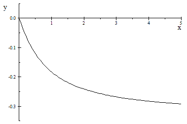
Figure 2: Graphic of the function $\beta=\beta\left(b\right)$.

Remark 5.12

In the original set of variables the self-similar solution has the form

$$g\left(t,w\right)=\frac{1}{t^{4}}G\left(\frac{w}{t}\right)$$

with $G$ as in Theorem 5.7.

Proof.

The existence of a real number $\beta$ and a measure $G$ satisfying (5.50) and solving (5.46) if $b$ is sufficiently large and $\frac{K}{b}$ is sufficiently small is just a consequence of Theorem 4.13 since under these assumptions $\left\|L\right\|$ in (5.47) is small.

It only remains to prove the asymptotics (5.51). To this end we describe in detail the solutions of the eigenvalue problem (5.48), (5.49). We denote $\lambda=\frac{\alpha}{b}+1.$ The problem (5.59), (5.60) has the following eigenvalues and eigenvectors

$$\lambda=0\ :\ \Gamma_{1,3}=\Gamma_{2,3}=\Gamma_{3,3}=0\ ;\ \Gamma_{1,1}+\Gamma_{2,2}=0\ ,\ \ \Gamma_{1,2}\text{ arbitrary}$$

$$\lambda=-\frac{1}{2b}\ :\ \Gamma_{1,2}=\Gamma_{3,3}=\Gamma_{1,1}=\Gamma_{2,2}=0\ ;\ \Gamma_{1,3},\ \Gamma_{2,3}\text{ arbitrary}.$$

Notice that the subspaces of eigenvectors of each of these eigenvalues have dimension two. The last remaining eigenvectors are

$$\lambda_{1} =\frac{1}{2}\left[-\left(B-1\right)+\sqrt{\left(B-1\right)^{2}+\frac{8}{3}B}\right]$$

$$\lambda_{2} =\frac{1}{2}\left[-\left(B-1\right)-\sqrt{\left(B-1\right)^{2}+\frac{8}{3}B}\right].$$

Since $\beta$ is given by the eigenvalue of (5.59), (5.60) with the largest real part, i.e. $\lambda_{1}$ we obtain (5.62). ∎

6 Conjectures on the non-self-similar behavior

We recall that, the collision operator in (1.6) is quadratic. It rescales like:

$$\rho\left(t\right)\left[w\right]^{\gamma}\left[g\right]\$$ (6.1)

where $\left[w\right]$ is the order of magnitude of $w$, $\gamma$ is the homogeneity of the collision kernel $B$ (cf. (2.4)) and $\left[g\right]$ the order of magnitude of $g$

The term $L\left(t\right)$ can yield different behaviors as $t\rightarrow\infty.$ We denoted the term $L\left(t\right)w\cdot\partial_{w}g$ as hyperbolic term. It can be constant, or it can behave like a power law (increasing or decreasing). As we pointed out in the introduction, the key idea is that there are three possibilities depending on the value of the homogeneity $\gamma$ and the function yielding the scaling of $\left[w\right].$ Either the hyperbolic term is larger than the collision term as $t\rightarrow\infty$, either the collision term is larger or either the hyperbolic term and the collision term have the same order of magnitude. Suppose that $L\left(t\right)$ scales like a function $\eta\left(t\right).$ The hyperbolic term scales then like $\eta\left(t\right)\left[g\right]$ and the collision term scales as in (6.1). Therefore, we need to compare the terms: $\eta\left(t\right)\text{ and }\rho\left(t\right)\left[w\right]^{\gamma}.$

In this section we give conjectures for the cases in which the hyperbolic term and the collision term do not balance. More precisely, the cases for which the hyperbolic terms dominate, and those in which the collision term dominates. We believe, based on formal calculations, that the latter can be handled by the Hilbert expansion, but using as small parameter $1/t$. These lengthy formal calculations are presented elsewhere [19], and here we give conjectures based on these calculations to complete most of the cases classified in Section 3. See Table 8 for these conjectures.

The cases in which the hyperbolic terms dominate have two subcases. In one subcase, according to a simplified model (presented in [19]), the collisions term is formally very small as $t\rightarrow\infty,$ but has a huge effect on the particle distributions. We do not make conjectures about this interesting subcase here. In the other subcase the hyperbolic terms are so dominant that the collisions have no effect on the asymptotic behavior of the solution (“frozen collisions”).

We describe a few details on these formal calculations below.

6.1 Collision-dominated behavior

As we discussed at the beginning of this section, we can have three different asymptotic behaviors for the solutions of (1.6) depending on the value of the homogeneity $\gamma$ and the function yielding the scaling of $\left[w\right].$ Here we focus on the case in which, for some values of $\gamma$, the collision term dominates the hyperbolic term. From now on, we refer to this case as the “collision-dominated behavior” case.

For collision-dominated behavior we have computed the asymptotics of the velocity dispersion using a suitable Hilbert expansion around the Maxwellian equilibrium. To formulate our conjecture based on this expansion we define for $t>0$

$$\mu(t)=\left\{\begin{array}[]{ll}1,&{\rm simple\ shear},\\ 1/t,&{\rm planar\ shear,\ or\ 2d\ dilatation,\ or\ combined\ shear},\\ \end{array}\right.$$ (6.2)

In the long time asymptotics, the solutions behave like a Maxwellian distribution with increasing or decreasing temperature depending on the sign of the homogeneity parameter $\gamma$.

Conjecture. Let $g\left(\cdot\right)\in C\left(\left[0,\infty\right]:\mathscr{M}_{+}\left(\mathbb{R}_{c}^{3}\right)\right)$ be a mild solution in the sense of Definition 4.1 of the Boltzmann equation with cross-section $B$ and let $\mu$ be defined in the various cases by (6.2). Then, for $t\to\infty$, the solution behaves like a Maxwellian distribution, i.e.

$$g(w,t)\to\tilde{C}\beta(t)^{\frac{3}{2}}e^{-\beta(t)\left|w\right|^{2}}\quad\text{in}\quad L^{2}\left(\mathbb{R}^{3};e^{-\left|w\right|^{2}}dw\right).$$ (6.3)

where $\tilde{C}=\frac{1}{(2\pi)^{\frac{3}{2}}}$. More precisely, we have the following cases.

• Assume that

  $$\operatorname{Tr}(L)\neq 0$$ (6.4)

  with $L$ as in (2.11). We define $a:=\frac{2}{3}\operatorname{Tr}(L)$. If $\mu(t)e^{-\frac{\gamma}{2}at}\to\infty$ the asymptotic behavior is given by a Maxwellian distribution (6.3) with

  $$\beta(t)=C\,e^{at}\quad{\rm as}\ \ t\to\infty,$$ (6.5)

  where $C>0$ is a numerical constant.

• Let $\gamma>0$ and assume that

  $$\int_{0}^{+\infty}\frac{ds}{\mu(s)}=\infty$$ (6.6)

  and

  $$\operatorname{Tr}(L)=0$$ (6.7)

  with $L$ as in (2.11). Then the asymptotic behavior is given by a Maxwellian distribution (6.3) with increasing temperature where $\beta(t)$ satisfies

  $$\beta(t)\simeq\left(\gamma\,b\int_{0}^{t}\frac{ds}{\mu(s)}\right)^{-\frac{2}{\gamma}}\quad\text{as}\quad t\to\infty$$ (6.8)

  with $b=-\left\langle\xi\cdot L\xi,(\mathbb{L})^{-1}[(\xi\cdot L\xi)])\right\rangle_{w}\,$ (Green-Kubo formula).

Further details about this conjecture can be found in [19]. We emphasize that in the case 1) with $\mu(t)=1$, in order to obtain a dynamics dominated by collisions, we must choose the homogeneity $\gamma$ satisfying the condition $a\cdot\gamma<0$.

6.2 Hyperbolic-dominated behavior

As mentioned at the beginning of this section we focus on the case of frozen collisions, i.e, that the collisions term becomes so small that the effect of collisions is irrelevant as $t\to\infty$. The formal argument underlying our conjectures is based on control of collision rate (gain term) for molecular densities that satisfy the asymptotic first order hyperbolic equation $\partial_{t}g+\partial_{w}\cdot(L(t)wg)=0$. If the resulting collision rate is decreasing in time, we refer to this case as hyperbolic-dominated behavior. More precisely, our terminology frozen collisions refers to the case of exponentially decreasing behavior of the collision rate as $t\to\infty$.

For frozen collisions we conjecture the following behavior.

1. Homogeneous dilatation: for $\gamma>-2$ the solution $g(t,w)$ converges in the sense of measures to a limit distribution that depends on the initial datum.

2. Cylindrical dilatation: for $\gamma>-2$ the solution $g(t,w)$ converges in the sense of measures to a limit distribution that depends on the initial datum.

3. Simple shear: for $\gamma<-1$ the solution $g(t,w)$ converges in the sense of measures to a limit distribution that depends on the initial datum.

Note that these regimes are complementary to those given by the formal Hilbert expansion and the self-similar profile, except the case of simple shear, for which there is a gap $-1\leq\gamma<0$. In this gap the collision rate is small but it still plays a significant role in the formal asymptotic behavior of the Boltzmann equation. A detailed justification for these conjectures can be found in [19].

7 Entropy formulas

Homoenergetic solutions are characterized by constant values in space of the particle density $\rho=\rho\left(t\right)$ and internal energy $\varepsilon=\varepsilon\left(t\right).$ We now discuss the form of another relevant thermodynamic magnitude, namely the entropy. We identify for the Boltzmann equation the entropy with minus the $H-$function. Then if the velocity distribution is given by $f=f\left(t,x,v\right),$ we obtain the following entropy density for particle at a given point $x$

$$\frac{s\left(x,t\right)}{\rho\left(t\right)}=-\frac{1}{\rho\left(t\right)}\int f\left(t,x,v\right)\log\left(f\left(t,x,v\right).\right)d^{3}v$$

It then readily follows, using (2.6) the entropy density for particle is independent of $x$ and given by

$$\frac{s\left(t\right)}{\rho\left(t\right)}=-\frac{1}{\rho\left(t\right)}\int_{\mathbb{R}^{3}}g\left(t,w\right)\log\left(g\left(t,w\right)\right)d^{3}w.$$ (7.1)

It is interesting to notice that in several of the solutions discussed above, the formulas for entropy for particle have many analogies with the corresponding formulas for equilibrium distributions, in spite of the fact that the distributions obtained in this paper deal with nonequilibrium situations.

The case in which the analogy between the entropy formulas for the equilibrium case and the considered solutions is the largest, nonsurprisingly, if the particle distribution is given by a Hilbert expansion (see details in [19]). However, there is also a large analogy between the entropy formulas of equilibrium distributions and self-similar solutions. This is due to the fact that to a large extent, the entropy formulas depend on the scaling properties of the distributions. Indeed, notice that both in the cases of solutions given by Hilbert distributions or self-similar solutions we can approximate $g\left(t,w\right)$ as

$$g\left(w,t\right)\sim\frac{1}{a\left(t\right)}G\left(\frac{w}{\lambda\left(t\right)}\right)\text{ as }t\rightarrow\infty$$ (7.2)

for suitable functions $a\left(t\right),\ \lambda\left(t\right)$ which are related to the particle density and the average energy of the particles. In the case of solutions given by Hilbert expansions the distribution $G$ is a Maxwellian, which can be assumed to be normalized to have density one and temperature one. Moreover, we will assume also that the mass of the particles is normalized to $m=2$ in order to get simpler formulas. This implies that the Maxwellian distribution takes the form $G_{M}(\xi)={\pi^{-\frac{3}{2}}}{e^{-|\xi|^{2}}}.$

In the case of the self-similar solutions considered in this paper, $G$ is a non Maxwellian distribution.

We define the energy for particle $e\left(t\right)$ as

$$\rho\left(t\right)e\left(t\right)=\varepsilon\left(t\right)=\int_{\mathbb{R}^{3}}\left|w\right|^{2}gdw.$$

Then, using the approximation (7.2)

$$\rho=\frac{\lambda^{3}}{a}\int G\left(\xi\right)d\xi\ ,\ \ e=\lambda^{2}\frac{\int\left|\xi\right|^{2}Gd\xi}{\int G\left(\xi\right)d\xi}.$$

Therefore

$$\frac{e^{\frac{3}{2}}}{\rho}=a\frac{\left(\int\left|\xi\right|^{2}Gd\xi\right)^{\frac{3}{2}}}{\left(\int G\left(\xi\right)d\xi\right)^{\frac{5}{2}}}$$

and

$$\log\left(\frac{e^{\frac{3}{2}}}{\rho}\right)=\log\left(a\right)+\log\left[\frac{\left(\int\left|\xi\right|^{2}Gd\xi\right)^{\frac{3}{2}}}{\left(\int G\left(\xi\right)d\xi\right)^{\frac{5}{2}}}\right].$$

On the other hand (7.1) yields

$$\frac{s}{\rho}=\log\left(a\right)-\frac{\int G\log\left(G\right)d\xi}{\int G\left(\xi\right)d\xi}.$$

Then

$$\frac{s}{\rho}=\log\left(\frac{e^{\frac{3}{2}}}{\rho}\right)+C_{G}$$ (7.3)

where $C_{G}$ is

$$C_{G}=-\frac{\int G\log\left(G\right)d\xi}{\int G\left(\xi\right)d\xi}-\log\left[\frac{\left(\int\left|\xi\right|^{2}Gd\xi\right)^{\frac{3}{2}}}{\left(\int G\left(\xi\right)d\xi\right)^{\frac{5}{2}}}\right].$$ (7.4)

The formula (7.3) has the same form as the usual formula of the entropy for the equilibrium case, except for the value of the constant $C_{G}.$ In the case of solutions given by Hilbert expansions the value of $C_{G}$ is the same as the one in the formula of the entropy for the equilibrium case. Therefore, in the case of the solutions obtained in this paper which can be approximated by Hilbert expansions, the asymptotic formula for the entropy by particle is the same as the one for the equilibrium case.

In the case of the self-similar solutions the value of the constant $C_{G}$ differs from the corresponding value for the one for the equilibrium case. Since the entropy tends to a maximum for a given value of the particle density and energy, it follows that $G_{G}<C_{M},$ where $C_{M}$ is the corresponding value of the constant for a Maxwellian distribution with density one and temperature one and it takes the value $C_{M}=\frac{3}{2}\big{[}1-\log\big{(}\frac{3}{2}\big{)}\big{]}$.

In the case of hyperbolic-dominated behavior the formula of the entropy for the corresponding solutions does not necessarily resemble the formula of the entropy for the equilibrium case, because in general the scaling properties of the particle distributions are very different from the ones taking place in the case of gases described by Maxwellian distributions. For further discussions in this direction we refer to [19].

8 Table of results

We collect here all the results obtained in this paper and in [19].

• Simple shear.

  The critical homogeneity corresponds to $\gamma=0$, i.e. to Maxwell molecules.

  Critical case              ($\gamma=0$)

  Supercritical case            ($\gamma>0$)

  Self-similar solutions with increasing temperature

  Maxwellian distribution with time dependent temperature    (Hilbert expansion)

  
  

• Homogeneous dilatation.

  The critical homogeneity corresponds to $\gamma=-2$.

  Critical case              ($\gamma=-2$)

  Subcritical case            ($\gamma<-2$)

  Maxwellian distribution with time dependent temperature    (Hilbert expansion)

  Maxwellian distribution with time dependent temperature    (Hilbert expansion)

• Planar shear.

  The critical homogeneity corresponds to $\gamma=0$, i.e. to Maxwell molecules.

  Critical case              ($\gamma=0$)

  Subcritical case            ($\gamma<0$)

  Self-similar solutions

  Maxwellian distribution with time dependent temperature    (Hilbert expansion)

• Planar shear with $K=0$.

  The critical homogeneity corresponds to $\gamma=0$, i.e. to Maxwell molecules.

  Critical case              ($\gamma=0$)

  Subcritical case            ($\gamma<0$)

  Self-similar solutions

  Maxwellian distribution with time dependent temperature    (Hilbert expansion)

• Cylindrical dilatation.

  In this case we have two critical homogeneities: $\gamma=-\frac{3}{2}$ and $\gamma=-{2}$.

  ($\gamma>-{2}$)

  ($\gamma<-\frac{3}{2}$)

  Frozen collisions

  Maxwellian distribution with time dependent temperature    (Hilbert expansion)

• Combined shear in orthogonal directions $(K_{1},K_{2},K_{3})$ with $K_{1}K_{3}\neq 0$.

  The critical homogeneity corresponds to $\gamma=0$, i.e. to Maxwell molecules.

  Critical case              ($\gamma=0$)

  Supercritical case            ($\gamma>0$)

  Non Maxwellian distribution

  Maxwellian distribution with time dependent temperature    (Hilbert expansion)

9 Conclusions

We have obtained several examples of long time asymptotics for homoenergetic flows of the Boltzmann equation. These flows yield a very rich class of possible behaviors. Homoenergetic flows can be characterized by a matrix $L\left(t\right)$ which describes the deformation taking place in the gas. The behavior of the solutions obtained in this paper depends on the balance between the hyperbolic terms of the equation, which are proportional to $L\left(t\right)$ and the homogeneity of the collision kernel. Roughly speaking the flows can be classified in three different types, which correspond to the situations in which the hyperbolic terms are the largest ones as $t\rightarrow\infty,$ the collision terms are the dominant ones and both of them have a similar order of magnitude respectively.

In this paper, we provided a rigorous proof of the existence of self-similar solutions yielding a non Maxwellian distribution of velocities in the case in which the hyperbolic terms and the collisions balance. A distinctive feature of these self-similar solutions is that the corresponding particle distribution does not satisfy a detailed balance condition. In these solutions the particle velocities are given by a subtle interplay between particle collisions and shear.

The solutions obtained in this paper yield interesting insights about the mechanical properties of Boltzmann gases under shear. On the other hand, the results of this paper suggest many interesting mathematical questions which deserve further investigation. We have obtained in several cases critical exponents for the homogeneity of the collision kernel. At the values of those critical exponents we expect to have self-similar velocities distributions. This has been proved rigorously in the cases in which the value of the critical homogeneity is zero, i.e. for Maxwell molecules. New methods are needed to prove the existence of self-similar solutions for critical homogeneities different from zero, as for instance we could expect in the case of cylindrical dilatation for the critical value of the homogeneity, i.e. $\gamma=-2$.

In the case of collision-dominated behavior and in the case of hyperbolic-dominated behavior we proposed some conjectures for asymptotic formulas for the solutions based on formal computations presented in [19]. In the first case we have obtained that the corresponding distribution of particle velocities for the associated homoenergetic flows can be approximated by a family of Maxwellian distributions with a changing temperature whose rate of change is obtained by means of a Hilbert expansion. It would be relevant to prove rigorously the existence of those solutions and to understand their stability properties.

In the case in which the hyperbolic terms are much larger than the collision terms the resulting solutions yield much more complex behaviors than the ones that we have obtained in the previous cases. The detailed understanding of the particle distributions is largely open and challenging.

Moreover, there are also homoenergetic flows yielding divergent densities or velocities at some finite time. These flows seem to have also interesting properties but we have not considered them in this paper.

Acknowledgements. We thank Stefan Müller, who motivated us to study this problem, for useful discussions and suggestions on the topic. The work of R.D.J. was supported by ONR (N00014-14-1-0714), AFOSR (FA9550-15-1-0207), NSF (DMREF-1629026), and the MURI program (FA9550-12-1-0458, FA9550-16-1-0566). A.N. and J.J.L.V. acknowledge support through the CRC 1060 The mathematics of emergent effects of the University of Bonn that is funded through the German Science Foundation (DFG).

References

- [1] A. V. Bobylev, Exact solutions of the Boltzmann equation. (Russian) Dokl. Akad. Nauk SSSR 225, 1296–1299 (1975)
- [2] A. V. Bobylev, A class of invariant solutions of the Boltzmann equation. (Russian) Dokl. Akad. Nauk SSSR 231, 571–574 (1976)
- [3] A. V. Bobylev, G. L. Caraffini, G. Spiga, On group invariant solutions of the Boltzmann equation. Journal Math. Phys. 37, 2787–2795 (1996)
- [4] A. V. Bobylev, I. M. Gamba, and V. Panferov. Moment inequalities and high-energy tails for the Boltzmann equations with inelastic interactions. J. Statist. Phys. 116(5-6), 1651–1682, (2004)
- [5] C. Cercignani, Mathematical Methods in Kinetic Theory. Plenum Press: New York, (1969)
- [6] C. Cercignani, Existence of homoenergetic affine flows for the Boltzmann equation. Arch. Rat. Mech. Anal. 105(4), 377–387, (1989)
- [7] C. Cercignani, Shear Flow of a Granular Material. J. Stat. Phys. 102(5),1407–1415, (2001)
- [8] C. Cercignani, The Boltzmann equation approach to the shear flow of a granular material. Philosophical Trans. Royal Society. 360, 437–451, (2002)
- [9] C. Cercignani, R. Illner, M. Pulvirenti, The Mathematical Theory of Dilute Gases. Springer, Berlin, (1994)
- [10] K. Dayal and R. D. James, Nonequilibrium molecular dynamics for bulk materials and nanostructures. Journal of the Mechanics and Physics of Solids 58, 145–163, (2010)
- [11] K. Dayal and R. D. James, Design of viscometers corresponding to a universal molecular simulation method. J. Fluid Mechanics 691, 461–486, (2012)
- [12] M. Escobedo, S. Mischler, and M. Rodriguez Ricard. On self-similarity and stationary problem for fragmentation and coagulation models. Ann. Inst. Henri Poincaré (C) Anal. Non Linéaire, 22 (1), 99–125, (2005)
- [13] M. Escobedo, J. J. L. Velázquez, On the theory of Weak Turbulence for the Nonlinear Schrödinger Equation. Memoirs of the AMS, 238, 1124, (2015)
- [14] V. S. Galkin, On a class of solutions of Grad’s moment equation. PMM, 22(3), 386–389, (1958). (Russian version PMM 20, 445-446, (1956)
- [15] V. S. Galkin, One-dimensional unsteady solution of the equation for the kinetic moments of a monatomic gas. PMM 28(1), 186–188, (1964)
- [16] V. S. Galkin, Exact solutions of the kinetic-moment equations of a mixture of monatomic gases. Fluid Dynamics (Izv. AN SSSR) 1(5), 41–50, (1966)
- [17] I. M. Gamba, V. Panferov, and C. Villani. On the Boltzmann equation for diffusively excited granular media. Comm. Math. Phys., 246(3), 503–541, (2004)
- [18] V. Garzó and A. Santos, Kinetic Theory of Gases in Shear Flows: Nonlinear Transport. Kluwer Academic Publishers, (2003)
- [19] R. D. James, S. Müller, A. Nota, J. J. L. Velázquez. Long time asymptotics for homoenergetic solutions of the Boltzmann equation for non Maxwell molecules. In preparation
- [20] T. Kato, Perturbation Theory for Linear Operators. Springer Verlag, Classics in Mathematics, (1976)
- [21] A. Kierkels, J. J. L. Velázquez. On the transfer of energy towards infinity in the theory of weak turbulence for the nonlinear Schrödinger equation. J. Stat. Phys. 159, 668–712, (2015)
- [22] B. Niethammer and J. J. L. Velázquez. Self-similar solutions with fat tails for Smoluchowski’s coagulation equation with locally bounded kernels. Comm. Math. Phys. 318(2), 505–532, (2013)
- [23] B. Niethammer, S. Throm, and J. J. L. Velázquez. Self-similar solutions with fat tails for Smoluchowski’s coagulation equation with singular kernels. Ann. Inst. Henri Poincaré (C) Nonlinear Analysis 33(5), 1223–1257, (2016)
- [24] A. A. Nikol’skii, On a general class of uniform motions of continuous media and rarefied gas. Soviet Engineering Journal 5(6), 757–760, (1965)
- [25] A. A. Nikol’skii, Three-dimensional homogeneous expansion-contraction of a rarefied gas with power-law interaction functions. DAN SSSR 151(3), (1963)
- [26] W. Rudin, Functional Analysis, McGraw-Hill, (1973)
- [27] C. Truesdell, On the pressures and flux of energy in a gas according to Maxwell’s kinetic theory, II. J. Rat. Mech. Anal. 5, 55–128 (1956)
- [28] C. Truesdell and R. G. Muncaster, Fundamentals of Maxwell’s Kinetic Theory of a Simple Monatomic Gas. Academic Press, (1980)
- [29] C. Villani, A review of mathematical topics in collisional kinetic theory. Hand-book of mathematical fluid dynamics, 1, 71–305, North-Holland, Amsterdam, (2002)
- [30] C. Villani, Topics in optimal transportation, vol. 58 of Graduate Studies in Mathematics. American Mathematical Society, Providence, RI, (2003)