Accelerating Energy Games Solvers
on Modern Architectures

Abstract

Quantitative games, where quantitative objectives are defined on weighted game arenas, provide natural tools for designing faithful models of embedded controllers. Instances of these games that recently gained interest are the so called Energy Games. The fast-known algorithm solves Energy Games in $\mathcal{O}(EVW)$ where $W$ is the maximum weight. Starting from a sequential baseline implementation, we investigate the use of massively data computation capabilities supported by modern Graphics Processing Units to solve the initial credit problem for Energy Games. We present four different parallel implementations on multi-core CPU and GPU systems. Our solution outperforms the baseline implementation by up to 36x speedup and obtains a faster convergence time on real-world graphs.

1 Introduction

Classic game theoretic-formulations of the control synthesis problem rely on two player zero-sum games on graphs, where the system is opposed to an antagonist environment. In this context, the modeling game arena is a graph, where the vertices are either owned by player $0$ (the system) or by the antagonist player $1$ (the environment). The two players move a pebble along the vertices of the graph, starting from an initial position. Whenever the pebble is on a vertex belonging to player $0$ (resp. player $1$), the latter decides where to move the pebble next, according to his strategy. The infinite path followed by the pebble is called a play and represents one possible behavior of the system. The winning objective for player $0$ (a set of plays) encodes exactly the acceptable behaviors of the system. Therefore, the goal of player $0$ is to ensure with his strategy—the synthesized controller—that the outcome of the game is an acceptable behavior of the system, whatever the strategy played by his adversary.

Quantitative games, where quantitative objectives are defined on weighted game arenas, provide natural tools for designing faithful models of embedded controllers, since they allow to explicitly handle the quantitative constraints imposed by the environment, the lack of resources or the targeted parameters of operability. In the late seventies, traditional game theory developed for economics defined a number of nowadays classic quantitative objectives, such as meanpayoff (MPG) and discounted-payoff [1, 26], that have been recently extensively investigated for the specification and design of reactive systems [1]. In turn, the problem of controller synthesis with resource constraints has inspired new quantitative objectives and quantitative games, such as e.g. so called energy games in [10, 4, 7] and their variants (see e.g. [12, 13, 16, 5, 25]). The latter turn out to be of broad interest, having applications in computer aided synthesis [12, 13, 8], real-time systems [6, 5], as well as economy, due to their connection with meanpayoff and discounted-sum objectives [1].

In energy games, edges are fitted with integer weights aimed at modeling rewards or costs. The objective of player $0$ is to maintain the sum of the weights (called the energy level) always positive along the play, given a fixed initial credit of energy. Energy games were introduced in [10, 4], where they were also proven memoryless determined: namely, each vertex is either winning for player $0$ or it is winning for player $1$, and memoryless strategies are sufficient to consider. Deciding whether a vertex $v$ is winning for player $0$ in an energy game is equivalent to the corresponding problem in meanpayoff games, and the latter equivalence has provided faster pseudo-polynomial algorithms for MPGs [7, 14, 15]. The above decision problems lie notoriously in the complexity class NP $\cap$ coNP (and even UP $\cap$ coUP), while finding polynomial time procedures for them is a long standing open problem [26, 1]. The minimum credit problem on energy game subsumes the corresponding decision problem, and asks the following: to determine, for each vertex $v$ of an energy game $\mathcal{G}$, whether $v$ is winning for player $0$ and which is the minimum credit to stay alive along each play starting from $v$. Such a problem can be also solved in pseudo-polynomial time [26, 7]. Recently, parallel architectures like Graphics Processing Units (GPU) have been successfully used in accelerating many irregulars and low-arithmetic intensity applications like graph traversal-based algorithms, in which the control flow and memory access patterns are data-dependent [9, 3]. Motivated by the large instances that naturally arise from the specification, design and control of reactive systems, in this work we investigate the use of massively data computation capabilities supported by modern GPUs for solving the initial credit problem on energy games. Also, to alleviate the workload unbalancing among threads, we propose a suitable data-thread mapping technique which allows to efficiently solve traditional Energy Games instances. The contributions of the paper are manifold:

• we provide a parallel implementation, exploiting traditional multi-core architectures, of the state-of-the-art initial credit procedure for enrgy games in [7];

• we developed a CUDA implementation which relies on a traditional vertex-parallelism approach and a more suitable variant based on warp-centric parallelism;

• we report experimental results where we compare the performance achieved by the above mentioned implementations and a completely sequential one.

After reviewing some minimal preliminary notions (Section 2), the theoretical results on Energy Games (EG) relevant for this paper are recalled in Section 3. Sections 4-5 describe our parallel solutions. The results of the experimentation activity and a comparison between the solvers are outlined in Section 6. We finally discuss related works in Section 7 and draw our conclusion in Section 8.

2 Preliminaries

Weighted graphs

A weighted graph is a tuple $G=(V,E,w)$, where $V$ is a set of of vertices, $E\subseteq V\times V$ is a set of edges, and $w:E\to{\mathbb{Z}}$ is a weight function assigning an integer weight to each edge. We assume that weighted graphs are total, i.e. for all $v\in V$, there exists $v^{\prime}\in V$ such that $(v,v^{\prime})\in E$. Given a set of vertices $U\subseteq V$ in a weighted graph $G=(V,E,w)$, we denote by ${\sf pre}(U)$ the set of vertices having a successor in $U$, i.e. ${\sf pre}(U)=\{v\mid\exists v^{\prime}\in U:(v,v^{\prime})\in E\}$, and by ${\sf post}(U)$ the set of successors of vertices in $U$, i.e. ${\sf post}(U)=\{v\mid\exists v^{\prime}\in U:(v^{\prime},v)\in E\}$.

A (finite) path $p$ in $G=(V,E,w)$ is a nonempty sequence of vertices $v_{0}v_{1}\dots$ (resp. $v_{0}v_{1}\dots v_{n}$) such that $(v_{i},v_{i+1})\in E$ for all $0\leq i$ (resp. $0\leq i<n$). The length of a finite path $p=v_{0}v_{1}\dots v_{n}$ is the number of vertices $n+1$ in $p$, denoted $|p|$. Given a (finite) path $p$ and an integer $j\geq 0$ (resp. $0\leq j\leq n$), we denote by $p^{j}$ the prefix $v_{0}\dots v_{j}$ of $p$ up to $j$ and by $p[j]$ the vertex $v_{j}$. A cycle in $G=(V,E,w)$ is a finite path $p=v_{0}v_{1}\dots v_{n}$ such that $n\geq 1$ and $v_{0}=v_{n}$. We say that a cycle in a weighted graph is negative (resp. nonnegative) if the sum of its edge weights is less than $0$ (resp. not less than $0$). Given $v\in V$, a cycle $v_{0}v_{1}\dots v_{n}$ is said reachable from $v$ in $G$ if there exists a path $u_{0}u_{1}\dots u_{m}$ in $G$ such that $u_{0}=v$ and $u_{m}=v_{0}$. A path $v_{0}v_{1}\dots v_{n}$ is acyclic if $v_{i}\neq v_{j}$ for all $0\leq i<j\leq n$.

Graph games

A game arena is a tuple $\Gamma=(V,E,w,\langle V_{0},V_{1}\rangle)$ where $G^{\Gamma}=(V,E,w)$ is a weighted graph and $\langle V_{0},V_{1}\rangle$ is a partition of $V$ into the set $V_{0}$ of player-$0$ vertices and the set $V_{1}$ of player-$1$ vertices. An infinite game on $\Gamma$ is played for infinitely many rounds by two players moving a pebble along the edges of the game arena $G^{\Gamma}$. In the first round, the pebble is on some vertex $v\in V$. In each round, if the pebble is on a vertex $v\in V_{i}$ ($i=0,1$), then player $i$ chooses an edge $(v,v^{\prime})\in E$ and the next round starts with the pebble on $v^{\prime}$. A play in the arena $\Gamma=(V,E,w,\langle V_{0},V_{1}\rangle)$ is an infinite path $\pi\subseteq V^{\omega}$ in $(V,E,w)$. An objective for player $0$ is a set $\mathcal{O}_{0}\subseteq V^{\omega}$: the play $\pi\in V^{\omega}$ is said to be winning for player $0$ if $\pi\in\mathcal{O}_{0}$. In this paper, we restrict our attention to $0$-sum games, i.e. games where the two players are antagonists: therefore, the objective of player $1$ is $\mathcal{O}_{1}=V^{\omega}\setminus\mathcal{O}_{0}$. A game is a tuple $\mathcal{G}=\langle\Gamma,\mathcal{O}_{0}\rangle$, where $\Gamma$ is a graph arena, and $\mathcal{O}_{0}\subseteq V^{\omega}$ is the objective of player $0$. Given a game $\langle\Gamma,\mathcal{O}_{0}\rangle$, the players play according to strategies to ensure a play that accomplish their objective.

A strategy for player $i$ ($i=0,1$) is a function $\sigma:V^{*}\cdot V_{i}\to V$, such that for all finite paths $v_{0}v_{1}\dots v_{n}$ with $v_{n}\in V_{i}$, we have $(v_{n},\sigma(v_{0}v_{1}\dots v_{n}))\in E$. We denote by $\Sigma_{i}$ ($i=0,1$) the set of strategies for player $i$. A strategy $\sigma$ for player $i$ is memoryless if $\sigma(p)=\sigma(p^{\prime})$ for all sequences $p=v_{0}v_{1}\dots v_{n}$ and $p^{\prime}=v^{\prime}_{0}v^{\prime}_{1}\dots v^{\prime}_{m}$ such that $v_{n}=v^{\prime}_{m}$. We denote by $\Sigma^{M}_{i}$ the set of memoryless strategies of player $i$. A play $v_{0}v_{1}\dots v_{n}\dots$ is consistent with a strategy $\sigma$ for player $i$ if $v_{j+1}=\sigma(v_{0}v_{1}\dots v_{j})$ for all positions $j\geq 0$ such that $v_{j}\in V_{i}$. Given an initial vertex $v\in V$, the outcome of two strategies $\sigma_{1}\in\Sigma_{1}$ and $\sigma_{2}\in\Sigma_{2}$ in $v$ is the (unique) play $\mathsf{outcome}^{\Gamma}(v,\sigma_{0},\sigma_{1})$ that starts in $v$ and is consistent with both $\sigma_{0}$ and $\sigma_{1}$. Given a memoryless strategy $\pi_{i}$ for player $i$ in the game $\mathcal{G}=\langle\Gamma,\mathcal{O}_{0}\rangle$, we denote by $G^{\Gamma}(\pi_{i})=(V,E_{\pi_{i}},w)$ the weighted graph obtained by removing from $G^{\Gamma}$ all edges $(v,v^{\prime})$ such that $v\in V_{i}$ and $v^{\prime}\neq\pi_{i}(v)$.

3 Energy Games

In this section, we introduce energy games [10, 4, 7], that are the main objective of the rest of this paper. An energy game is a game $\mathcal{G}=\langle\Gamma,\mathcal{O}_{0}\rangle$ over the arena $\Gamma=(V,E,w,\langle V_{0},V_{1}\rangle)$, where the goal of player $0$ is to construct an infinite play $v_{0}v_{1}\dots v_{n}\dots$ such that for some initial credit $c\in\mathbb{N}$, it holds that:

$$c+\sum_{i=0}^{j}w(v_{i},v_{i+1})\geq 0\text{ for all }j\geq 0$$ (1)

The quantity $c+\sum_{i=0}^{j-1}w(v_{i},v_{i+1})$ in (1) is called the energy level of the play prefix $v_{0}v_{1}\dots v_{j}$, given the initial credit $c$. Conversely, player $1$ aims at building a play $\pi=v_{0}v_{1}\dots v_{n}\dots$ such that for any initial credit $c$, there exists a prefix $\pi^{j}$ of $\pi$ such that the energy level of $\pi^{j}$ is negative. Formally, energy games are defined as follows:

Definition 1 (Energy Games)

An energy game (EG) is a game $\mathcal{G}=\langle\Gamma,\mathcal{O}_{0}\rangle$, where $\Gamma=(V,E,w,\langle V_{0},V_{1}\rangle)$ and $\mathcal{O}_{0}$ is given by:

$$\begin{array}[]{l}\mathcal{O}_{0}\,=\{\pi|\>\pi\mbox{ is a path in $G^{\Gamma}=\langle V,E,w\rangle$}\,\wedge\\ \phantom{\mathcal{O}_{0}\,=\{\pi|\>}\exists c\in\mathbb{N}:c+\sum_{i=0}^{j-1}w(v_{i},v_{i+1})\geq 0\text{ for all }j\geq 0\}\end{array}$$

A vertex $v\in V$ is winning for player $i$, $i\in\{0,1\}$ if there exists an initial credit $c(v)$ and a winning strategy for player $i$ from $v$ for credit $c(v)$. In the sequel, we denote by $W_{i}$ the set of winning vertices for player $i$.

Energy games are memoryless determined [4], i.e. for all $v\in V$, either $v$ is winning for player $0$, or $v$ is winning for player $1$, and memoryless strategies are sufficient. Using the memoryless determinacy of energy games, one can easily prove the following result for EG, characterizing the winning strategies for player $0$ in a EG.

Lemma 2 ([7])

Let $\mathcal{G}=\langle\Gamma,\mathcal{O}_{0}\rangle$ be an EG, for all vertices $v\in V$, for all memoryless strategies $\pi_{0}\in\Sigma^{M}_{0}$ for player $0$, the strategy $\pi_{0}$ is winning from $v$ iff all cycles reachable from $v$ in the weighted graph $G^{\Gamma}(\pi_{0})$ are nonnegative.

Example 3

Consider the energy game depicted in Figure 1, where round vertices are owned by player $0$, and square vertices are owned by player $1$. The set of winning vertices for player $0$ is $W_{0}=V$. In fact, the memoryless strategy $\sigma_{0}:V_{0}\rightarrow V$ for player $0$, where $\sigma_{0}(1)=\sigma_{0}(3)=4$, ensures that any cycle in a play consistent with $\sigma_{0}$—against any (memoryless) strategy $\sigma_{1}$ for player $1$—is nonnegative. Therefore, provided a suitable initial credit of energy, each play consistent with $\sigma_{0}$ will enjoy a nonnegative energy level along its run. Given $v\in W_{0}=V$, the minimum initial credit $c(v)$ that player $0$ needs to survive along a play starting from $v$ is given by $c:W_{0}\rightarrow\mathbb{N}$, where $c(1)=2,c(2)=2,c(3)=1,c(4)=1$. As a further example, if the edge $(3,4)$ is deleted from the energy game in Figure 1, then player $0$ does not have any winning strategy from $W_{1}=\{2,3\}$, but only from the set of vertices $W_{0}=\{1,4\}$ with initial credit of energy $c(1)=1,c(4)=0$.

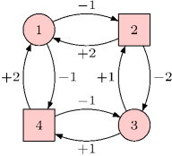
Figure 1: An Energy Game $\mathcal{G}$.

The next definition introduces the initial credit problem.

Definition 4 (Initial Credit Problem)

Given an energy game $\mathcal{G}=\langle\Gamma,\mathcal{O}_{0}\rangle$, the initial credit problem on $\mathcal{G}$ asks to determine, for each vertex $v\in V$, the following:

1. if $v$ is winning for player $0$, i.e. if $v\in W_{0}$.

2. in case $v\in W_{0}$, the minimum initial credit ${\sf c}(v)$ such that there is a winning strategy $\sigma_{0}$ for player $0$ in $\mathcal{G}$.

The decision problem for an energy game $\mathcal{G}=\langle\Gamma,\mathcal{O}_{0}\rangle$ asks to solve only the first one of the two items above, i.e. to partition $V$ into $\langle W_{0},W_{1}\rangle$. The decision problem on energy games is equivalent to the decision problem on so called meanpayoff games [26], a game on graphs originally introduced by game theorists within the economic community, where the objective of player $0$ is to minimize the long-run average weight of plays. Several algorithms exist to solve the decision problem on meanpayoff games (cf. [1] for a survey of the available algorithms): indeed, it is worth noticing that the best pseudo-polynomial meanpayoff algorithm is based on its reduction to energy games [7, 14, 15]. Ad-hoc procedures are instead necessary to solve the initial credit problem on energy games, that is specific to energy objectives. The latter problem was solved in [7] with a pseudo-polynomial procedure having complexity $\mathit{\mathcal{O}(\lvert E\rvert{\cdot}\lvert V\rvert{\cdot}W)}$, where $\lvert E\rvert$ (resp. $\lvert V\rvert$) is the number of edges in the game arena and $W$ is the maximum weight labeling an edge. Energy games were algorithmically studied also in [14], where the authors provide a polynomial algorithm for solving the initial credit problem on EG with special weights structures. In particular, the authors of [14] show that solving EG where all the cycles are either ’good’ or significantly ‘bad’ can be done in polynomial time.

In the rest of this paper, we will show the design of a CUDA-based parallel EG algorithm based on the procedure for the EG initial credit problem defined in [7] (which is briefly described in the next subsection). The latter allows to exploit the computational power offered by modern GPUs.

3.1 Computing the Minimum Initial Credit of Energy on the CPU

In this subsection, we briefly describe the sequential algorithm in [7] to solve the initial credit problem on energy games. The procedure in [7] is based on the of so called energy progress measure, which is recalled in Definition 5 and relies on the following notation.

Let $\preceq$ be the total order on $\mathcal{N}=\mathbb{N}\cup\{\top\}$, where $x\preceq y$ if and only if either $x\leq y$ or $y=\top$. Let $\ominus$ be the operator $\ominus:\mathcal{N}\times{\mathbb{Z}}\to\mathcal{N}$ such that, for each $a\in\mathcal{N}$ and $b\in{\mathbb{Z}}$:

$$a\ominus b=\left\{\begin{array}[]{ll}\max(0,a-b)&\mbox{if $a\neq\top$ }\\ \top&\mbox{otherwise}\end{array}\right.$$

Roughly speaking, the local conditions on the nodes of an energy game $\mathcal{G}$ imposed by an energy progress measure $f$ (cf. Definition 5) guarantee that the following property on $\mathcal{G}$ holds: for each node $v$ in $\mathcal{G}$, if $f(v)\neq\top$, then player $0$ has a strategy $\sigma_{0}$ to ensure that the energy level along each play compatible with $\sigma_{0}$ is not negative, provided the initial credit $f(v)$.

Definition 5 (Energy Progress Measure (EPM) [7])

A function $f:V\to\mathcal{N}$ is a energy progress measure for the EG $\mathcal{G}=\langle\Gamma,\mathcal{O}_{0}\rangle$ iff the following conditions hold:

• if $v\in V_{0}$, then $f(v)\succeq f(v^{\prime})\ominus w(v,v^{\prime})$ for some $(v,v^{\prime}){\in}E$

• if $v\in V_{1}$, then $f(v)\succeq f(v^{\prime})\ominus w(v,v^{\prime})$ for all $(v,v^{\prime})\in E$

For a game $\mathcal{G}$, let ${\mathcal{F}}$ be the set of functions $f:V\to\mathcal{N}$, and consider the partial order $\sqsubseteq\subseteq{\mathcal{F}}\times{\mathcal{F}}$, defined as $f\sqsubseteq g$ iff for all $v\in V$, $f(v)\preceq g(v)$. The authors of [7] proved that $\mathcal{G}$ admits a least energy progress measure $f$ w.r.t. $\sqsubseteq$, satisfying the following properties:

1. for each node $v\in W_{1}$, $f(v)=\top$

2. for each node $v\in V_{0}$, $f(v)\leq\mathcal{M}_{G}$, where:

   $$\mathcal{M}_{\mathcal{G}}=\sum_{v\in V}\max(\{0\}\cup\{-w(v,v^{\prime})\mid(v,v^{\prime})\in E\})$$

Given an EG $\mathcal{G}$, the initial energy credit algorithm in [7] computes exactly the least energy progress measure for $\mathcal{G}$:

$$f:V\to\mathcal{C}_{\mathcal{G}}=\{n\in\mathbb{N}\mid n\leq\mathcal{M}_{\mathcal{G}}\}\cup\{\top\}.$$

More precisely, such an algorithm initializes $f$ to the constant function $0$ and relies on the following $\sqsubseteq$-monotone lifting operator to update $f$, until a least fixpoint is reached.

begin  /* Initialize the set $L$ of nodes for which the least EPM $f$ needs to be lifted */

$L\leftarrow\{v\in V_{0}\mid\forall(v,v^{\prime})\in E:w(v,v^{\prime})<0\}$ ;

$L\leftarrow L\cup\{v\in V_{1}\mid\exists(v,v^{\prime})\in E:w(v,v^{\prime})<0\}$ ;

/* Initialize the least EPM $f$ */

foreach $v\in V$ do  $f(v)\leftarrow 0$ ;

if $v\in V_{0}\cap L$ then ${\sf count}(v)\leftarrow 0$ ;

if $v\in V_{0}\setminus L$ then ${\sf count}(v)\leftarrow\lvert\{v^{\prime}\in{\sf post}(v)\mid f(v)\geq f(v^{\prime})\ominus w(v,v^{\prime})\}\rvert$ ;

/* Apply the lift-operator to update the least EPM $f$ for each node in $L$ */

while $L\neq\emptyset$ do  Pick $v\in L$ ;

$L\leftarrow L\setminus\{v\}$;

$old\leftarrow f(v)$ ;

$f\leftarrow\delta(f,v)$ ;

if $v\in V_{0}$ then ${\sf count}(v)\leftarrow\lvert\{v^{\prime}\in{\sf post}(v)\mid f(v)\geq f(v^{\prime})\ominus w(v,v^{\prime})\}\rvert$ ;

foreach $v^{\prime}\in{\sf pre}(v)$ such that $f(v^{\prime})<f(v)\ominus w(v^{\prime},v)$ do  if $v^{\prime}\in V_{0}$ then  if $f(v^{\prime})\geq old\ominus w(v^{\prime},v)$ then ${\sf count}(v^{\prime})\leftarrow{\sf count}(v^{\prime})-1$ ;

if ${\sf count}(v^{\prime})\leq 0$ then $L\leftarrow L\cup\{v^{\prime}\}$ ;

if $v^{\prime}\in V_{1}$ then $L\leftarrow L\cup\{v^{\prime}\}$ ;

return $f$ ;

end

Algorithm 1 Minimum Initial Credit Algorithm for Energy Games: Given in input an EG $\mathcal{G}$, it computes in output the least progress measure $f:V\to\mathcal{C}_{\mathcal{G}}$

18

18

18

18

18

18

18

18

18

18

18

18

18

18

18

18

18

18

Definition 6 (Lifting Operator [7])

Given $v\in V$, the lifting operator $\delta(\cdot,v):[V\to\mathcal{C}_{\mathcal{G}}]\to[V\to\mathcal{C}_{\mathcal{G}}]$ is defined by $\delta(f,v)=g$ where:

$$g(u)=\left\{\begin{array}[]{ll}f(u)&\mbox{if $u\neq v$}\\ \min\{f(v^{\prime})\ominus w(v,v^{\prime})\mid(v,v^{\prime})\in E\}&\mbox{if $u=v\in V_{0}$}\\ \max\{f(v^{\prime})\ominus w(v,v^{\prime})\mid(v,v^{\prime})\in E\}&\mbox{if $u=v\in V_{1}$}\end{array}\right.$$

To conclude this subsection we report in Algorithm 1 the exact pseudo-code of the minimum initial credit algorithm in [7], based on the least energy progress measure described above. Such an algorithm uses suitable counters to achieve a global worst-case complexity of $\mathcal{O}(\lvert E\rvert\cdot\mathcal{M}_{\mathcal{G}})$=$\mathit{\mathcal{O}(\lvert E\rvert{\cdot}\lvert V\rvert{\cdot}W)}$.

4 An OpenMP implementation

In order to obtain an immediate way to parallelize the computation of the minimum initial credit on EG , let us observe that each application of the lift operation in Definition 6 never decreases the value of $f(v)$ for any vertex $v$. Hence, processing all elements in $L$ in parallel is a sound procedure. Moreover, as motivated in the previous subsection, a bounded number $\lvert E\rvert\cdot\mathcal{M}_{\mathcal{G}}$ of lift operations suffices to determine a solution. Consequently, a simple way to parallelize the computation of the EPM consists in applying the lift operation in parallel for each vertex of the graph and in iterating this step until either a fixpoint or the theoretical bound on loops is reached. Algorithm 2 presents the skeleton of the resulting algorithm implemented exploiting OpenMP. In particular, the loops starting in lines 1 (performing the initialization of $f$) and 8 (performing the lift step), respectively, are executed in parallel by distributing the computation among the available OpenMP threads. The while-loop in lines 5–10 iterates until an ending condition is achieved. We experimented with this implementation by using 1, 2, 4, and 8 threads, always mapped to different CPUs (see Section 6).

begin  /* Initialize the least EPM $f$ */

foreach $v\in V$ in parallel do  $f(v)\leftarrow 0$; $loops\leftarrow\lvert E\rvert\cdot\mathcal{M}_{\mathcal{G}};\hfill\mbox{\tt/* Bound on number of lifts */}$

$more\leftarrow true$;

/* Apply lift-operator until fixpoint or the bound on loops is reached */

while $more\wedge loops>0$ do  $f^{\prime}\leftarrow f$;

$loops\leftarrow loops-1$;

foreach $v\in V$ in parallel do  $f{\leftarrow}\delta(f,v);\hfill\mbox{\tt/* Each thread lifts a $v$ */}$

$more{\leftarrow}more{\vee}f(v)\not=f^{\prime}(v)$; /* Race condition*/ return $f$; end

Algorithm 2 Naive parallel version of Algorithm 1

11

11

11

11

11

11

11

11

11

11

11

5 A CUDA-Based Solver

begin  /* Initialize the least EPM $f$ and the set $L$ of nodes to be lifted */

foreach $v\in V$ in parallel do  $f(v)\leftarrow 0$;

if $(v\in V_{0}\wedge(\forall(v,v^{\prime})\in E:w(v,v^{\prime})<0))$ $\vee$ $(v\in V_{1}\wedge(\exists(v,v^{\prime})\in E:w(v,v^{\prime})<0))$ then $L\leftarrow L\cup\{v\}$;

/* Apply lift-operator until a fixpoint */

while $L\not=\emptyset$ do  $L^{\prime}\leftarrow\emptyset$;   $f^{\prime}\leftarrow f;\hfill\mbox{\tt/* done in parallel */}$

foreach $v\in L$ in parallel do  $f{\leftarrow}\delta(f,v);\hfill\mbox{\tt/* Each thread lifts one $v$ */}$

if $f(v)\not=f^{\prime}(v)$ then  foreach $v^{\prime}\in{\sf pre}(v)$ do $L^{\prime}\leftarrow L^{\prime}\cup\{v^{\prime}\}$;

$L\leftarrow L^{\prime};\hfill\mbox{\tt/* done in parallel */}$ return $f$ ;

end

Algorithm 3 CUDA Algorithm for Energy Games

11

11

11

11

11

11

11

11

11

11

11

This section describes the main design choices made in implementing a CUDA-based parallel solution to the EG initial credit problem. As concerns data structures, the adjacency matrix of the input EG is represented in device memory, by exploiting the standard Compressed Sparse Row (CSR) format, usually employed to store sparse matrices. The progress measure $f$ to be computed is stored in an array of $|V|$ elements.

By analyzing the pseudo-code of the sequential Algorithm 1, one plainly identifies tasks that could be executed in parallel. The simplest one is the initialization of the set $L$ of active nodes (those whose least energy progress measure $f$ needs to be lifted) and the initialization of the least progress measure $f$ (lines 1-3 in Algorithm 3). The set $L$ is represented by an array of (at most) $|V|$ elements, A specific kernel function has been defined for the initialization of such $L$. In particular, a 1-to-1 mapping (vertex-parallelism  [19]) assigns each node to one thread. Each thread determines whether the corresponding node has to be inserted in $L$ or not (line 3).

The core of the sequential algorithm is in lines 7–17, where elements are extracted from $L$, one at a time, and their progress measures are lifted. As mentioned before, processing all elements in $L$ in parallel is a sound procedure. Therefore, a specific kernel function has been designed to compute, in parallel, the new values of $f(v)$ for each $v$ in $L$. In doing this, all elements $v^{\prime}$ in the set ${\sf post}(v)$ have to be considered. To better exploit the mass parallelism supported by GPUs, each node $v$ in $L$ is assigned to a set of $h=2^{k}$ threads of the same warp. Such threads process in parallel all elements in ${\sf post}(v)$ and (conjunctively) compute the value of $\delta(f,v)$. Information between such threads is exchanged through warp-shuffle operations, which are enabled because all $h$ threads always belong to the same warp. Acting in this manner reduces the number of accesses to global and shared memories and this, in turn, speeds-up the overall computation. Indeed, as mentioned earlier, by means of shuffle operations data are moved directly between threads’ registers instead of communicating them through global/shared memory operations. The value $h$ can be heuristically chosen as (a fraction of) the average degree of nodes in $V$.

Thanks to the use of the CSR format, all members of ${\sf post}(v)$ are stored in consecutive locations of the device memory. This optimizes the time needed by the $h$ threads for accessing the initially needed data. The first of the $h$ threads stores the new value of $f(v)$, after the interaction between the $h$ threads is completed.

Consider now that, by Definition 6, the computation of lifting operator involves the evaluation of either a $\min$ operation or a $\max$ operation of a set of values, depending on the player controlling the active node. A further optimization is applied in order to minimize thread divergence between threads of the same warp. The set $V$ is sorted so that all nodes in $V_{0}$ (resp. $V_{1}$) correspond to consecutive lines of the adjacency matrix of the EG. Consequently, in all warps (but at most one) all threads always execute the same sequence of instructions. Namely, all of them compute the $\min$ (resp. $\max$) operation.

Once the progress measure $f(v)$ of a node $v$ has been updated, the set of predecessors ${\sf pre}(v)$ of $v$ has to be considered in order to compute the new set of active nodes. Also this task is performed in parallel by splitting the work load among the $h$ threads. The set of $h$ threads that computed $\delta(f,v)$, process each node in ${\sf pre}(v)$ and determine if it has to be inserted in $L$. Notice that in this phase of the computation it might be the case that the same element might be inserted in the new $L$ because of different reasons, as it is predecessor of different processed active nodes. Repeated insertion of the same element in $L$ is avoided by marking each inserted node (a suitable vector of flags is used for this purpose).

Similarly to what done in computing $\delta(f,v)$, in order to optimize the access patterns exploited to retrieve the needed data, the elements of ${\sf pre}(v)$ are stored in consecutive memory locations. This is achieved by adopting a redundant representation of $E$. More specifically, the adjacency matrix of EG is represented in the device memory using the Compressed Sparse Column (CSC) format too. This representation is easily computed by transposing the corresponding CSR representation, through standard functions provided by the CUSPARSE library.

With the differences described so far, the overall structure of the resulting CUDA implementation essentially reflects the one of the sequential Algorithm 1. The computation starts on the CPU by reading and parsing a text file specifying the input arena. The EG is then transferred to the device memory and a conversion from CSR to CSC is executed by the device. Now, the CPU controls the computation by calling the device functions described earlier. First the initialization of data is performed. Then, the device function which improves the progress measure is repeatedly called until an empty set of active nodes is obtained (this corresponds to the while-loop in Algorithm 1). We experimented with different choices for the values of $h$ (the case $h=1$ clearly corresponds to vertex-parallelism, while for $h>1$ we have warp-centric parallelism). Finally, the result is transferred back to the host memory and output.

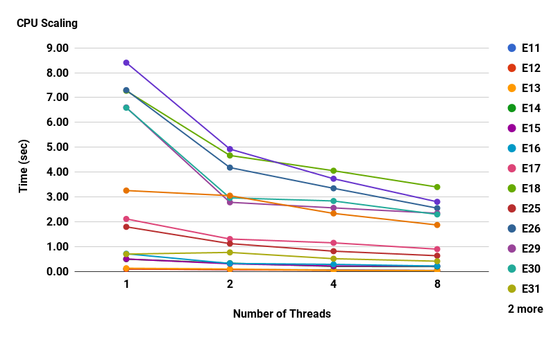
(a) Dataset: Equivalence Checking.

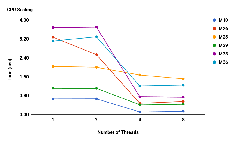
(b) Dataset: Model Checking.

Figure 2: CPU EG scaling experiment. The figures report the performance in seconds (y-axis) required to solve Energy Games instances by increasing the number of threads on Intel Xeon E5-2640 (x-axis).

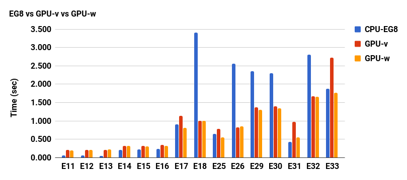
Figure 3: Performance comparison among three different parallel implementations CPU-EG8, GPU-v and GPU-w on Equivalence Checking data set. The bars show the time-to-solution in seconds of each implementation.

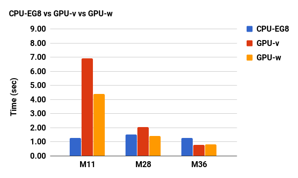
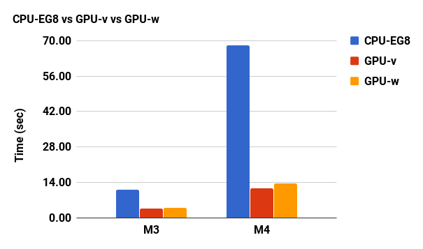
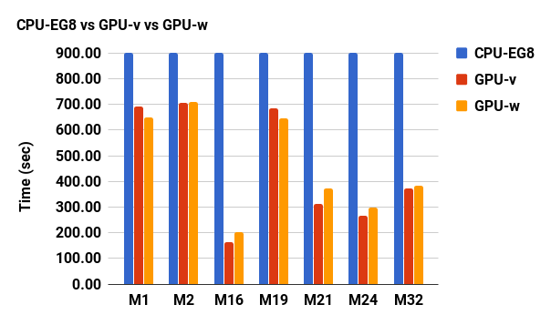
Figure 4: Performance comparison among three different parallel implementations CPU-EG8, GPU-v and GPU-w on Equivalence Checking data set. The bars show the time-to-solution in seconds of each implementation.

6 Experimental Results

Numerical experiments have been performed on a server equipped with an Intel Xeon E5-2640 v3 and four Nvidia K80 GPU. The code has been generated using the GNU C compiler version 4.8.2, CUDA C compiler version 7.5.

A sequential solver, named “CPU EG1”, following the pseudo-code listed in Algorithm 1 has been implemented in C. In order to develop a fair comparison with the GPU-based solution, the very same representation (using both CSR and CSC formats) used in the CUDA implementation has been adopted in the sequential solver. We refer to “CPU EG2”, “CPU EG4” and “CPU EG8” the codes that implement the algorithm described in Algorithm 2 with 2,4,8 threads respectively.

The codename “GPU-v” and “GPU-w” denote the code implemented for GPUs based on vertex parallelism and warp parallelism respectively. As a source for our benchmark, we consider the suite for games arena in [20]. In particular, [20] provides a large database of games (over $1000$ instances) that originate from different verification problems and are notable—for experimental purposes—in terms of their diversity and applicative coverability. Table 1 provides references to the filenames of the exact instances used in the experimentation as well as a succinct description of the characteristics of the graphs. Such instances encode equivalence checking ($E0$-$E33$) model-checking ($M0$-$36$) problems into qualitative games with parity objectives [1]. Standard conversion from qualitative games to quantitative games with meanpayoff and energy objectives [7] have been used in [22] to generate the final data set.

Performance Analysis

In the present section, we show our experimental results. First, we compared the performance of CPU-EG over the data set by increasing the number of threads (strong scaling). Due to slow convergence time, CPU-EG is not able to solve some instances within a given time-out (for our convenience we set up it to 900 seconds). In Figure 2 we only show the most representative results. Please refer to Table 1 for a detailed analysis. In general, experiments show a good scalability between 2 and 4 threads, after that threads do not have enough work to do. For some instances (i.e., M33), CPU-EG shows a better scalability since it takes advantage from the parallelism that a more complex structure exhibits. Other instances, like M28, on the contrary, do not have a significant benefit from multi-core architectures.

In the second set of experiments, we compare the performance (time-to-solution) between GPU-v and GPU-w. Furthermore, we also show the time of CPU-EG8 as a baseline. In detail, Figure 3 shows the performance over “equivalence checking” data set, whereas Figure 4 is related to “model checking” instances. Generally, CPU-EG8 is faster on “easy” instances where the algorithm converges quickly in few iterations. The identification of “easy” instances is hard to do a priori since, as we mentioned, the convergence strongly depends on the weights and the structure of the graphs. By analyzing final performance we can say that EG-GPUs are up to $5$x than CPU-EG8 (36x faster than EG-CPU1). Concerning the comparison between GPU-v and GPU-w, we do not observe a significant difference in terms of performance except for a small number of instance. On average, GPU-w achieves better performance slightly up to a factor of $1.7$x.

As a final comment, the results of this initial experimentation seem to witness the advantages offered even by a plain parallelization of Algorithm 1. Although our results are remarkable, a deeper investigation has to be conducted in order to identify (if any) those classes of EG where a specific approach may achieve the best performance. Again, it seems reasonable that particular topologies of the underlying graph game may reduce the gap between the sequential and the parallel algorithms. On the other hand, various optimizations and refinements can be introduced in the parallel solver. Among the ones under consideration we just mention here the possibility of partitioning the given arena w.r.t. the strongly connected components of the graph game and processing them in parallel, just by imposing a topological order among the components.

Graph ID Nodes Edges Avg Degree CPU EG1 CPU EG2 CPU EG4 CPU EG8 GPU-v GPU-w ABP(BW)_Onebit_(datasize=2_capacity=1_windowsize=1)eq=branching-bisim.sol E0 12239050 33790242 2.76 900.000 900.000 900.000 900.000 0.673 0.547 ABP(BW)_Onebit_(datasize=2_capacity=1_windowsize=1)eq=branching-sim.sol E1 12239050 33790242 2.76 900.000 900.000 900.000 900.000 0.557 0.554 ABP(BW)_Onebit_(datasize=2_capacity=1_windowsize=1)eq=weak-bisim.sol E2 10685466 40545186 3.79 900.000 900.000 900.000 900.000 0.617 0.558 ABP(BW)_Onebit_(datasize=3_capacity=1_windowsize=1)eq=branching-bisim.sol E3 40556396 112380248 2.77 900.000 900.000 900.000 900.000 1.384 1.480 ABP(BW)_Onebit_(datasize=3_capacity=1_windowsize=1)eq=branching-sim.sol E4 40556396 112380248 2.77 900.000 900.000 900.000 900.000 1.331 1.481 ABP(BW)_Onebit_(datasize=3_capacity=1_windowsize=1)eq=weak-bisim.sol E5 35431922 134886692 3.81 900.000 900.000 900.000 900.000 1.542 1.670 ABP_Onebit_(datasize=2_capacity=1_windowsize=1)eq=branching-bisim.sol E6 9488018 26181506 2.76 900.000 900.000 900.000 900.000 0.473 0.396 ABP_Onebit_(datasize=2_capacity=1_windowsize=1)eq=branching-sim.sol E7 9488018 26181506 2.76 900.000 900.000 900.000 900.000 0.461 0.396 ABP_Onebit_(datasize=3_capacity=1_windowsize=1)eq=branching-bisim.sol E8 31611530 87556070 2.77 900.000 900.000 900.000 900.000 1.073 1.078 ABP_Onebit_(datasize=3_capacity=1_windowsize=1)eq=branching-sim.sol E9 31611530 87556070 2.77 900.000 900.000 900.000 900.000 1.095 1.075 ABP_Onebit_(datasize=3_capacity=1_windowsize=1)eq=weak-bisim.sol E10 27799634 104694734 3.77 900.000 900.000 900.000 900.000 1.235 1.307 Buffer_Onebit_(datasize=2_capacity=2_windowsize=1)eq=branching-bisim.sol E11 912641 2762529 3.03 0.116 0.087 0.074 0.050 0.204 0.193 Buffer_Onebit_(datasize=2_capacity=2_windowsize=1)eq=branching-sim.sol E12 912641 2762529 3.03 0.109 0.083 0.058 0.051 0.205 0.202 Buffer_Onebit_(datasize=2_capacity=2_windowsize=1)eq=weak-bisim.sol E13 966897 3278913 3.39 0.142 0.110 0.060 0.045 0.209 0.221 Buffer_Onebit_(datasize=3_capacity=2_windowsize=1)eq=branching-bisim.sol E14 3471553 11083645 3.19 0.507 0.345 0.215 0.209 0.311 0.310 Buffer_Onebit_(datasize=3_capacity=2_windowsize=1)eq=branching-sim.sol E15 3471553 11083645 3.19 0.513 0.321 0.231 0.226 0.310 0.296 Buffer_Onebit_(datasize=3_capacity=2_windowsize=1)eq=weak-bisim.sol E16 3644173 12968893 3.56 0.724 0.333 0.297 0.228 0.338 0.311 CABP_Onebit_(datasize=2_capacity=1_windowsize=1)eq=strong-bisim.sol E17 7626354 30467442 4.00 2.123 1.316 1.162 0.909 1.133 0.804 CABP_Onebit_(datasize=3_capacity=1_windowsize=1)eq=strong-bisim.sol E18 24812174 100409150 4.05 7.275 4.674 4.061 3.405 0.996 0.997 Hesselink_(Implementation)_Hesselink_(Specification)_(datasize=2)eq=branching-bisim.sol E19 33702306 76550466 2.27 900.000 900.000 900.000 900.000 0.996 0.996 Hesselink_(Implementation)_Hesselink_(Specification)_(datasize=2)eq=branching-sim.sol E20 33702306 76550466 2.27 900.000 900.000 900.000 900.000 1.038 1.011 Hesselink_(Implementation)_Hesselink_(Specification)_(datasize=2)eq=weak-bisim.sol E21 29868274 78747250 2.64 900.000 900.000 900.000 900.000 1.023 0.939 Hesselink_(Specification)_Hesselink_(Implementation)_(datasize=2)eq=branching-bisim.sol E22 33702306 76550466 2.27 900.000 900.000 900.000 900.000 0.983 1.033 Hesselink_(Specification)_Hesselink_(Implementation)_(datasize=2)eq=branching-sim.sol E23 33702306 76550466 2.27 900.000 900.000 900.000 900.000 0.995 1.006 Hesselink_(Specification)_Hesselink_(Implementation)_(datasize=2)eq=weak-bisim.sol E24 29868274 78747250 2.64 900.000 900.000 900.000 900.000 1.002 0.922 Onebit_SWP_(datasize=2_capacity=1_windowsize=1)eq=strong-bisim.sol E25 5322498 21604226 4.06 1.805 1.131 0.827 0.644 0.786 0.543 Onebit_SWP_(datasize=3_capacity=1_windowsize=1)eq=strong-bisim.sol E26 19026506 78220622 4.11 7.300 4.187 3.354 2.557 0.825 0.849 Par_Onebit_(datasize=2_capacity=1_windowsize=1)eq=branching-bisim.sol E27 10927074 30319218 2.78 900.000 900.000 900.000 900.000 0.514 0.427 Par_Onebit_(datasize=2_capacity=1_windowsize=1)eq=branching-sim.sol E28 10927074 30319218 2.78 900.000 900.000 900.000 900.000 0.526 0.426 SWP_SWP_(datasize=2_capacity=1_windowsize=2)eq=branching-bisim.sol E29 37636481 120755185 3.21 6.604 2.791 2.567 2.352 1.372 1.305 SWP_SWP_(datasize=2_capacity=1_windowsize=2)eq=branching-sim.sol E30 37636481 120755185 3.21 6.593 2.970 2.845 2.305 1.402 1.342 SWP_SWP_(datasize=2_capacity=1_windowsize=2)eq=strong-bisim.sol E31 3782172 11533061 3.05 0.710 0.777 0.525 0.424 0.966 0.551 SWP_SWP_(datasize=2_capacity=1_windowsize=2)eq=weak-bisim.sol E32 32926785 167527601 5.09 8.404 4.931 3.739 2.812 1.669 1.661 SWP_SWP_(datasize=3_capacity=1_windowsize=2)eq=strong-bisim.sol E33 14808231 45377590 3.06 3.264 3.058 2.345 1.880 2.720 1.773 BRPdatasize=2_counting.sol M0 2177202 2532590 1.16 0.758 0.751 0.191 0.213 0.274 0.273 Clobberwidth=4_height=4_black_has_winning_strategy.sol M1 564914 2185853 3.87 900.000 900.000 900.000 900.000 690.284 648.927 Clobberwidth=4_height=4_white_has_winning_strategy.sol M2 564914 2185853 3.87 900.000 900.000 900.000 900.000 705.454 708.674 Hanoindisks=12_eventually_done.sol M3 531443 1594321 3.00 66.898 66.567 12.706 11.051 3.510 3.928 Hanoindisks=13_eventually_done.sol M4 1594325 4782967 3.00 489.584 482.419 68.811 68.164 11.757 13.450 Hesselinkdatasize=2_nodeadlock.sol M5 540737 1115713 2.06 0.010 0.009 0.002 0.002 0.179 0.175 Hesselinkdatasize=2_property1.sol M6 1081474 2231426 2.06 0.071 0.072 0.057 0.059 0.218 0.211 Hesselinkdatasize2_property1.sol M7 1081474 2231426 2.06 0.072 0.071 0.070 0.060 0.221 0.208 Hesselinkdatasize=2_property2.sol M8 1093761 2246401 2.05 0.020 0.021 0.003 0.003 0.195 0.184 Hesselinkdatasize=3_nodeadlock.sol M9 13834801 29028241 2.10 0.353 0.355 0.058 0.058 0.455 0.395 Hesselinkdatasize=3_property2.sol M10 27876961 58309201 2.09 0.664 0.669 0.113 0.142 0.711 0.713 IEEE1394nparties=2_datasize=2_headersize=2_acksize=2_property4.sol M11 571378 996970 1.75 0.433 0.423 0.820 1.261 6.926 4.373 IEEE1394nparties=2_datasize=2_headersize=2_acksize=2_property5.sol M12 1411274 2454775 1.74 0.022 0.021 0.005 0.003 0.191 0.187 Lift_(Incorrect)nlifts=4_nodeadlock.sol M13 998790 5412890 5.42 0.192 0.189 0.153 0.165 0.237 0.241 Lift_(Incorrect)nlifts=4_safety_1.sol M14 788879 4146139 5.26 0.051 0.051 0.006 0.005 0.199 0.200 Onebitdatasize=3_invariantly_infinitely_many_reachable_taus.sol M15 867889 4933009 5.68 0.096 0.096 0.020 0.019 0.208 0.207 Onebitdatasize=3_messages_read_are_inevitably_sent.sol M16 579745 3354841 5.79 900.001 900.000 900.000 900.000 162.310 201.437 Onebitdatasize=3_no_duplication_of_messages.sol M17 1191962 6907934 5.80 0.126 0.124 0.163 0.158 0.253 0.261 Onebitdatasize=3_no_spontaneous_messages.sol M18 1278433 7843609 6.14 0.080 0.080 0.008 0.009 0.234 0.230 Onebitdatasize=3_read_then_eventually_send.sol M19 1350433 7068673 5.23 900.000 900.000 900.000 900.000 685.262 644.088 SWPdatasize=2_windowsize=3_infinitely_often_receive_for_all_d.sol M20 588868 2071109 3.52 0.189 0.196 0.039 0.039 0.198 0.197 SWPdatasize=2_windowsize=3_invariantly_infinitely_many_reachable_taus.sol M21 670177 2375809 3.55 900.000 900.000 900.000 900.000 311.157 373.967 SWPdatasize=2_windowsize=3_no_duplication_of_messages.sol M22 944090 3685946 3.90 0.124 0.126 0.069 0.071 0.366 0.269 SWPdatasize=2_windowsize=3_read_then_eventually_send_if_fair.sol M23 586658 1782434 3.04 0.059 0.060 0.017 0.018 0.191 0.200 SWPdatasize=2_windowsize=3_read_then_eventually_send.sol M24 917713 3283153 3.58 900.000 900.000 900.000 900.000 265.119 298.995 SWPdatasize=2_windowsize=4_infinitely_often_receive_d1.sol M25 3487362 12463874 3.57 1.211 1.207 0.232 0.235 0.329 0.331 SWPdatasize=2_windowsize=4_infinitely_often_receive_for_all_d.sol M26 6974724 24927749 3.57 3.277 2.539 0.481 0.555 0.478 0.482 SWPdatasize=2_windowsize=4_nodeadlock.sol M27 2589057 11565569 4.47 0.095 0.094 0.015 0.014 0.267 0.262 SWPdatasize=2_windowsize=4_no_duplication_of_messages.sol M28 11488274 45840722 3.99 2.038 2.004 1.677 1.515 2.047 1.388 SWPdatasize=2_windowsize=4_read_then_eventually_send_if_fair.sol M29 7310722 22667778 3.10 1.116 1.111 0.418 0.442 0.428 0.433 SWPdatasize=4_windowsize=2_infinitely_often_receive_for_all_d.sol M30 653574 2444297 3.74 0.220 0.218 0.045 0.047 0.204 0.200 SWPdatasize=4_windowsize=2_no_duplication_of_messages.sol M31 858114 3433490 4.00 0.062 0.062 0.058 0.057 0.281 0.235 SWPdatasize=4_windowsize=2_read_then_eventually_send.sol M32 869569 3200129 3.68 900.000 900.000 900.000 900.000 371.087 381.734 SWPdatasize=4_windowsize=3_infinitely_often_receive_d1.sol M33 8835074 34391042 3.89 3.683 3.706 0.757 0.737 0.618 0.658 SWPdatasize=4_windowsize=3_nodeadlock.sol M34 7429633 32985601 4.44 0.309 0.313 0.030 0.043 0.445 0.446 SWPdatasize=4_windowsize=3_no_generation_of_messages.sol M35 6690605 29413398 4.40 0.292 0.292 0.046 0.039 0.432 0.429 SWPdatasize=4_windowsize=3_read_then_eventually_send_if_fair.sol M36 24565250 73675010 3.00 3.110 3.293 1.212 1.249 0.779 0.790

Table 1: Dataset characteristics and experimental results. The first four columns show the instance name, a short ID used in the paper to refer to them, as well as some characteristics of the graphs such as size and vertex degrees. The rightmost six columns report the timings obtained by the different implementations described in the paper. In particular, the four columns labeled “CPU EG$n$”, list the results obtained by the sequential Algorithm 1 implemented in C (“CPU EG1”), and by its OpenMP version (Algorithm 2) for different number of threads (namely, for $n=2,4,8$). The columns “GPU-v” and “GPU-w” show the results obtained by the CUDA based solver (cf., Algorithm 3), exploiting a pure vertex parallelism and warp parallelism, respectively. All timings are in seconds. A timeout of 15 minutes has been applied (the values $900.000$ denote timeout expiration).

7 Related Works

Similar approaches exist for other kind of games used in the context of computer aided design and formal verification. For instance, the parallelization of Meanpayoff Games has been dealt with in [11] and in [17]. Whereas in the first case the target architecture is not GPU-based, but it is a common multi-core machine, [17] proposes an OpenCL implementation suitable to run on AMD devices. A proposal concerning Parity Games has been described in [22], also based on OpenCL.

Several solutions have been proposed to reduce the workload unbalancing among threads and alleviate the irregular memory access. Jia et al. [19] evaluated two different data-thread mapping techniques vertex-parallel and edge-parallel. Due to the difference in the out-degree among vertices in scale-free networks, vertex-parallel suffers from load imbalance among threads. The edge-parallel approach solves that problem by assigning edges to threads during the frontier expansion. However, it is not suitable for graphs with a low average degree, as well as dense graphs [19]. Furthermore, the edge-based parallelism requires much memory and atomic operations [19, 24] especially for Energy Games instances where an atomic min can be required. Mclaughlin and Bader [21] discussed two hybrid methods for the selection of the parallelization strategy. Sarıyüce et al. [23], introduced the vertex virtualization technique based on a relabeling of the data structure (e.g., CSR, Compressed Sparse Row). The technique replaces a high-degree vertex v with $n_{v}=\lceil\texttt{adj(v)}\rceil/\Delta$ virtual vertices having at most $\Delta$ neighbors. Vertex virtualization technique is not very effective for graphs with a low average degree. Typical Energy Games instances are characterized by a low average out degree (cfr. Table  1), therefore a vertex-based parallelism would be more suitable for such instances. Other efficient data-thread mapping techniques, like active-edge parallelism [2, 3] or other warp-centric strategies [18], seem to be not very effective for Energy games instances where the average degree is pretty low.

8 Concluding Remarks

To the best of our knowledge, we present the first GPU-based implementation of a solver for Energy Games. We investigated the possibility of implementing a solver for the initial credit problem on Energy Games capable of exploiting the computational power offered by modern Graphics Processing Units. We illustrated how a first prototype relying on the SIMT conceptual model of parallelism adopted within CUDA framework can be plainly obtained by parallelizing the different steps of a sequential algorithm. The proposed CUDA-based solver tersely exhibits great performance and demonstrated the viability of the approach, when compared against its sequential and CPU multi-core counterpart. However, a detailed analysis of the topology of the graph is still required in order to design an efficient data-thread mapping technique on GPUs. Further, a number of improvements and heuristics can be applied to our current implementation, involving for example a static analysis of the input instance aimed at customizing the configuration parameters used to launch the CUDA kernels, or aimed at taking advantage of the topological structure of the graph. These are challenging themes for future work.

References

- [1] K. Apt and E. Gradel. Lectures in Game Theory for Computer Scientists. Cambridge University Press, USA, 2011.
- [2] M. Bernaschi, G. Carbone, E. Mastrostefano, and F. Vella. Solutions to the st-connectivity problem using a gpu-based distributed bfs. Journal of Parallel and Distributed Computing, 76:145 – 153, 2015. Special Issue on Architecture and Algorithms for Irregular Applications.
- [3] M. Bernaschi, G. Carbone, and F. Vella. Scalable betweenness centrality on multi-gpu systems. In Proc. of CF’16, pages 29–36, USA, 2016. ACM.
- [4] P. Bouyer, U. Fahrenberg, K. G. Larsen, N. Markey, and J. Srba. Resource interfaces. In Proc. of FORMATS, volume 5215 of LNCS, pages 33–47. Springer, 2008.
- [5] P. Bouyer, N. Markey, M. Randour, K. Larsen, and S. Laursen. Average-energy games. In Proc. of GandALF, pages 1–15, 2015.
- [6] R. Brenguier, F. Cassez, and J.-F. Raskin. Energy and mean-payoff timed games. In Proc. of HSCC’14, pages 283–292, New York, NY, USA, 2014. ACM.
- [7] L. Brim, J. Chaloupka, L. Doyen, R. Gentilini, and J. Raskin. Faster algorithms for mean-payoff games. Formal Methods in System Design, 38(2):97–118, 2011.
- [8] V. Bruyère. Computer aided synthesis: a game theoretic approach. CoRR, 2017.
- [9] M. Burtscher, R. Nasre, and K. Pingali. A quantitative study of irregular programs on gpus. In Workload Characterization (IISWC), 2012 IEEE Int. Symposium on, pages 141–151. IEEE, 2012.
- [10] A. Chakrabarti, L. de Alfaro, T. Henzinger, and M. Stoelinga. Resource interfaces. In Proc. of EMSOFT:Embedded Software, volume 2855 of LNCS, pages 117–133. Springer, 2003.
- [11] J. Chaloupka. Parallel algorithms for mean-payoff games. In A. Fiat and P. Sanders, editors, Proc. of ESA 2009, volume 5757 of LNCS, pages 599–610, 2009.
- [12] K. Chatterjee and L. Doyen. Energy parity games. In Proc. of ICALP, volume 6199 of LNCS, pages 599–610. Springer, 2010.
- [13] K. Chatterjee, L. Doyen, T. Henzinger, and J.-F. Raskin. Generalized mean-payoff and energy games. In Proc. of FSTTCS, volume 8 of LIPIcs, pages 505–516, 2010.
- [14] K. Chatterjee, M. Henzinger, S. Krinninger, and D. Nanongkai. Polynomial-time algorithms for energy games with special weight structures. Algorithmica, 70(3), 2014.
- [15] C. Comin and R. Rizzi. Improved pseudo-polynomial bound for the value problem and optimal strategy synthesis in mean payoff games. Algorithmica, 77(4):995–1021, 2017.
- [16] U. Fahrenberg, L. Juhl, K. Larsen, and J. Srba. Energy games in multiweighted automata. In Proc. of ICTAC, volume 6916 of LNCS, pages 95–115. Springer, 2011.
- [17] P. Hoffmann and M. Luttenberger. Solving parity games on the GPU. In D. Van Hung and M. Ogawa, editors, Proc. of ATVA 2013, volume 8172 of LNCS, pages 455–459, 2013.
- [18] S. Hong, S. K. Kim, T. Oguntebi, and K. Olukotun. Accelerating cuda graph algorithms at maximum warp. In Proceedings of the 16th ACM Symposium on Principles and Practice of Parallel Programming, PPoPP ’11, pages 267–276, New York, NY, USA, 2011. ACM.
- [19] Y. Jia, V. Lu, J. Hoberock, M. Garland, and J. Hart. Edge vs. node parallelism for graph centrality metrics. GPU Computing Gems: Jade Edition, pages 15–28, 2011.
- [20] J. Keiren. Benchmarks for parity games. In M. Dastani and M. Sirjani, editors, Proc. of FSEN 2015. Revised Selected Papers, volume 9392 of LNCS, pages 127–142, 2015.
- [21] A. McLaughlin and D. Bader. Scalable and high performance betweenness centrality on the gpu. In Proc. of the Int. Conference for High Performance Computing, Networking, Storage and Analysis, pages 572–583. IEEE Press, 2014.
- [22] P. Meyer and M. Luttenberger. Solving mean-payoff games on the GPU. In C. Artho, A. Legay, and D. Peled, editors, Proc. of ATVA 2016, volume 9938 of LNCS, 2016.
- [23] A. Sariyüce, K. Kaya, E. Saule, and U. Çatalyürek. Betweenness centrality on gpus and heterogeneous architectures. In Proc. of GPGPU-6, pages 76–85, New York, NY, USA, 2013. ACM.
- [24] A. Sarıyüce, E. Saule, K. Kaya, and Ü. Çatalyürek. Regularizing graph centrality computations. J. of Parallel and Distributed Computing, 76(0):106 – 119, 2015. Special Issue on Architecture and Algorithms for Irregular Applications.
- [25] Y. Velner, K. Chatterjee, L. Doyen, T. Henzinger, A. Rabinovich, and J. Raskin. The complexity of multi-mean-payoff and multi-energy games. Inf. Comput., 241:177–196, 2015.
- [26] U. Zwick and M. Paterson. The complexity of mean payoff games on graphs. TCS, 158(2):343–359, 1996.