Ultrasonic waves in classical gases

Abstract

The velocity and absorption coefficient for the plane sound waves in a classical gas are obtained by solving the Boltzmann kinetic equation, which describes the reaction of the single-particle distribution function to a periodic external field. Within the linear response theory, the nonperturbative dispersion equation valid for all sound frequencies is derived and solved numerically. The results are in agreement with the approximate analytical solutions found for both the frequent- and rare-collision regimes.

March 18, 2024

I Introduction

Sound waves in classical gases have been studied intensively within the hydrodynamical approach (see, e.g., Ref. LLv6 ). Small dynamical perturbations of the particle density $n({\bf r},t)$, collective velocity ${\bf u}({\bf r},t)$, and temperature $T({\bf r},t)$ induced by sound-wave propagation are found as solutions of the hydrodynamical and transport equations. The sound velocity is approximately equal to the thermal particle velocity

$$v_{T}\leavevmode\nobreak\ =\leavevmode\nobreak\ \sqrt{\frac{2\,T}{m}}\leavevmode\nobreak\ ,$$ (1)

where $T$ is the system temperature and $m$ is the particle mass. For absorbed plane sound waves (APSWs) with a frequency $\omega$, the wave amplitude decreases as $\exp(-\gamma z)$ after propagating the distance $z$. The absorption coefficient $\gamma$ is obtained from the Stokes relation LLv6 . It is a function of the shear and bulk viscosity and the thermal conductivity.

Within a hydrodynamic approach, the kinetic coefficients are phenomenological constants. For their calculations, one needs kinetic theory. For classical systems of particles, the Boltzmann kinetic equation (BKE) is usually used. It describes the single-particle distribution function $f({\bf r},{\bf p},t)$ dependent on the space coordinate ${\bf r}$, momentum ${\bf p}$, and time $t$ (see, e.g., Refs. chapman ; kogan ; silin ; LPv10 ; reichl ; cercignani ; gorenstein ). The two lowest moments of the single-particle distribution give

$$n({\bf r},t)\leavevmode\nobreak\ = \leavevmode\nobreak\ \int d{\bf p}\leavevmode\nobreak\ f({\bf r},{\bf p},t)\leavevmode\nobreak\ ,$$

$${\bf u}({\bf r},t)\leavevmode\nobreak\ = \leavevmode\nobreak\ \frac{1}{n({\bf r},t)}\,\int d{\bf p}\leavevmode\nobreak\ \frac{{\bf p}}{m}\leavevmode\nobreak\ f({\bf r},{\bf p},t)\leavevmode\nobreak\ .$$ (2)

Chapman and Enskog (see, e.g., Ref. chapman ) derived the equations of a dissipative hydrodynamics by using the BKE. They obtained the expressions for the kinetic coefficients in the system of hard balls within the so-called frequent-collision regime (FCR) (see also Ref. MGGPprc16 ). To define the collision regimes, let us introduce two different scales: the particle mean free path $l\sim(n\pi d^{2})^{-1}$, where $d$ is the hard-core particle diameter, and another scale $L$ that is the characteristic space size of the external dynamical perturbation. In our APSW problem, one can set $L=\lambda$, where $\lambda=2\pi\,v_{T}/\omega$ is the wavelength of the propagating plane waves. The FCR corresponds to $l\ll\lambda$ and the perturbation expansion over a small Knudsen parameter ${\mathcal{K}}\equiv\omega\tau\ll 1$ can be used. Here, $\tau\sim l/v_{T}$ is the relaxation time that determines the collision frequency $\tau^{-1}$ by the collision integral term in the BKE. In most practical cases, the inequality $l\ll\lambda$ is satisfied, and the FCR works (see, e.g., Ref. LPv10 ). For example, for air at normal conditions one has $l\sim 10^{-5}$cm and $\lambda\sim 1-10^{3}$cm for audible sound waves. (For investigations within the FCR but beyond the standard hydrodynamic approach; see, for instance, Refs. Gr65book ; kogan ; cercignani ; abrkhal ; Gr65book ; Si65 ; GrJa59 ; BrFe66 ; brooksyk ; Le78 ; Wo79 ; Wo80 ; relkinbook ; woodsbook93 ; Le89 ; Ha01 ; spiegel_Ultrasonic_01 ; spiegel_BVKE-visc_03 ; smith05 ; AWprc12 ; AWcejp12 ; wiranata-jp-14 ; kapusta .)

The rare-collision regime (RCR) takes place at large values of the Knudsen parameter ${\mathcal{K}}=\omega\tau\gg 1$. The conditions of the RCR emerge at a small particle-number density ($l$ becomes large) and (very) large sound-wave frequency $\omega$. Different approximations were employed in this case kogan ; silin ; cercignani ; Si65 ; GrJa59 ; BrFe66 ; brooksyk ; Le78 ; Wo79 ; Wo80 ; relkinbook ; bhatia ; Le89 ; woodsbook93 ; magkohofsh ; Ha01 ; spiegel_Ultrasonic_01 ; pethsmith02 ; spiegel_BVKE-visc_03 ; smith05 ; KMprc06 ; litovitz ; review ; BMRprc15 . Most of them, e.g., kogan ; cercignani ; Si65 ; BrFe66 ; brooksyk ; Le78 ; Wo79 ; Wo80 ; relkinbook ; Le89 ; woodsbook93 ; Ha01 ; spiegel_Ultrasonic_01 ; spiegel_BVKE-visc_03 , used the so-called moments’ method based on a truncation of the system of equations for the moments of the BKE. However, a dynamical variation $\delta f({\bf r},{\bf p},t)$ of the distribution function $f({\bf r},{\bf p},t)$ becomes strongly oscillating and a nonsmooth function of the momentum ${\bf p}$ at large $\omega\tau\;\hbox{\kern 1.00006pt\lower 3.01385pt\hbox{$\sim$} \kern-11.19997pt\raise 2.15277pt\hbox{$>$} \kern 1.00006pt}1$. Therefore, in the RCR at $\omega\tau\;\hbox{\kern 1.00006pt\lower 3.01385pt\hbox{$\sim$} \kern-11.19997pt\raise 2.15277pt\hbox{$>$} \kern 1.00006pt}1$ the moments’ method fails, the worse the larger $\omega\tau$ (see, e.g., Refs. cercignani ; relkinbook ).

The APSWs in the RCR will be referred to as ultrasonic waves litovitz ; bhatia . The basic experiments in the field of ultrasonic waves were done by Greenspan (see Refs. Gr49 ; Gr56 ; Gr65book , and also Ref. Me57 for additional experimental data). After that no essential improvements of experimental measurements have been done. This is connected with serious difficulties in conducting these experiments. The difficulties include the problems of generating ultrasonic waves in gases and of measuring the speed and absorption of these waves.

Both the FCR and RCR have been studied in our recent paper MGGpre17 by using the approximate analytical solutions obtained within asymptotic expansions of the BKE over $\omega\tau\ll 1$ and $(\omega\tau)^{-1}\ll 1$, respectively. The aim of the present paper is to formulate the nonperturbative method for calculations of the speed of sound waves and the absorption coefficient $\gamma$ of the APSWs within the linear response theory (LRT) (for different aspects of the LRT see, e.g., Refs. kubo ; zubarev ; hofmann , and also Refs. magkohofsh ; review for its applications). The LRT allows us to derive a general APSW solution for small variations $\delta f({\bf r},{\bf p},t)$ of the distribution function $f$ in terms of the response of $\delta f$ to a periodic external field with a frequency $\omega$ by using the relaxation time approximation to the collision integral term. This can be done for any Knudsen parameter value $\mathcal{K}$, which is an essential advantage over the moments’ method. The equation for the poles of these response functions is the dispersion equation for the complex wave number $k$ (or the complex sound velocity), which allows us to obtain the sound velocity and the absorption coefficient.

The paper is organized as follows. In Sec. II, the Boltzmann kinetic equation with an external periodic field is formulated, and the relaxation time approximation for the collision integral is discussed. In Sec. III, the linearized BKE is solved in terms of the response to the external periodic potential. The nonperturbative dispersion equation for the complex wave numbers (sound velocities) of the APSWs is derived. Numerical solutions of this equation give the sound velocity and absorption coefficient of the APSWs at arbitrary values of the Knudsen parameter $\omega\tau$. The obtained numerical results are in agreement with the analytical RCR and FCR asymptotic limits. Sections  IV and V present, respectively, a discussion of the results and a summary. Appendixes A-C show some details of the calculations.

II Boltzmann Kinetic equation

We start with the BKE

$$\frac{\partial f}{\partial t}\leavevmode\nobreak\ +\leavevmode\nobreak\ \frac{{\bf p}}{m}\frac{\partial f}{\partial{\bf r}}\leavevmode\nobreak\ -\mbox{St}[f]\leavevmode\nobreak\ =\leavevmode\nobreak\ \frac{\partial f}{\partial{\bf p}}\;\frac{\partial V_{\rm ext}}{\partial{\bf r}}\;,$$ (3)

where the collision integral term $\mbox{St}[f]$ is taken in the standard Boltzmann form (see, e.g., Refs. kogan ; silin ; cercignani ; reichl ). The external potential field $V_{\rm ext}(z,t)$, periodic in time $t$ with a frequency $\omega$, is switched on as a perturbation

$$V_{\rm ext}(z,t)=\exp\left[-i\,\omega\,t+\epsilon_{0}t\right]\int_{-\infty}^{\infty}\frac{\mbox{d}k}{2\pi}\leavevmode\nobreak\ V_{k}\;\exp\left(ikz\right)\;,$$ (4)

where $V_{k}$ is the $k$ amplitude of the Fourier representation $\epsilon_{0}=+0$. The external field stimulates the appearance of the plane waves with a fixed frequency $\omega$. The term $\epsilon_{0}t$, switching adiabatically on the external field at a time far in the past ($V_{\rm ext}\rightarrow 0$ at $t\rightarrow-\infty$) , is used usually for the adequate time-dependent picture kubo ; zubarev , and will be omitted in the following derivations. For convenience, we use also the standard Fourier integral transformation of the LRT from the $z$ to $k$ variables.

In the absence of the external field $V_{\rm ext}$, the global equilibrium (GE) solution of the BKE (3) is given by

$$f_{\rm GE}(p)\leavevmode\nobreak\ =\leavevmode\nobreak\ \frac{n}{(2\pi mT)^{3/2}}\,\exp\left(-\;\frac{p^{2}}{2mT}\right)\;,$$ (5)

where the particle number density $n$ and temperature $T$ are independent of the spatial coordinates ${\bf r}$ and time $t$, $p\equiv|{\bf p}|$. Therefore, Eq. (5) for $f_{\rm GE}$ describes the homogeneous particle distribution in the coordinate space and the Maxwell distribution in the momentum space. This distribution satisfies Eq. (I) with $n({\bf r},t)=n$ and ${\bf u}({\bf r},t)=0$.

Let us define now small deviations $\delta f({\bf r},{\bf p},t)$ from the distribution function $f_{\rm GE}(p)$ ($|\delta f|/f_{\rm GE}\ll 1$),

$$\delta f({\bf r},{\bf p},t)\leavevmode\nobreak\ \equiv\leavevmode\nobreak\ f({\bf r},{\bf p},t)\leavevmode\nobreak\ -\leavevmode\nobreak\ f_{\rm\rm GE}(p)\;.$$ (6)

They arise from a small external potential $|V_{\rm ext}|/T\ll 1\leavevmode\nobreak\$. The linearized BKE (3) can be then written as

$$\frac{\partial\delta f}{\partial t}+\frac{{\bf p}}{m}\frac{\partial\delta f}{\partial{\bf r}}-\delta\mbox{St}[f]\leavevmode\nobreak\ \leavevmode\nobreak\ \leavevmode\nobreak\ \leavevmode\nobreak\ \leavevmode\nobreak\ \leavevmode\nobreak\ \leavevmode\nobreak\ \leavevmode\nobreak\ \leavevmode\nobreak\ \leavevmode\nobreak\ \leavevmode\nobreak\ \leavevmode\nobreak\ \leavevmode\nobreak\ \leavevmode\nobreak\ \leavevmode\nobreak\ \leavevmode\nobreak\ \leavevmode\nobreak\ \leavevmode\nobreak\ \leavevmode\nobreak\ \leavevmode\nobreak\ \leavevmode\nobreak\ \leavevmode\nobreak\ \leavevmode\nobreak\ \leavevmode\nobreak\ \leavevmode\nobreak\ \leavevmode\nobreak\ \leavevmode\nobreak\ \leavevmode\nobreak\ \leavevmode\nobreak\ \leavevmode\nobreak\ \leavevmode\nobreak\ \leavevmode\nobreak\ \leavevmode\nobreak\ \leavevmode\nobreak\ \leavevmode\nobreak\$$

$$=-i\frac{p_{z}}{mT}\;f_{\rm GE}\,\exp\left(-i\leavevmode\nobreak\ \omega t\right)\;\!\!\int_{-\infty}^{\infty}\frac{\mbox{d}k}{2\pi}\,k\,V_{k}\;\exp\left(ikz\right).$$ (7)

We can present $\delta f({\bf r},{\bf p},t)$ defined by Eq. (6) in terms of the sum of two terms

$$\delta f\leavevmode\nobreak\ \equiv\leavevmode\nobreak\ \delta f_{\rm LE}\leavevmode\nobreak\ +\leavevmode\nobreak\ \delta\varphi\leavevmode\nobreak\ .$$ (8)

The local equilibrium term $\delta f_{\rm LE}$ (see Ref. silin ) in Eq. (8) will be written as

$$\delta f_{\rm LE}\leavevmode\nobreak\ =\leavevmode\nobreak\ f_{\rm GE}\,\left(\frac{\delta n}{n}\leavevmode\nobreak\ +\leavevmode\nobreak\ \frac{p_{z}\delta u_{z}}{T}\right)\;,$$ (9)

where $\delta n$ and $\delta u_{z}$ are small deviations of the particle number density and collective velocity ($|\delta n|/n\ll 1$ and $|\delta u_{z}|/v_{T}\ll 1$) from their GE values $n$ and $u_{z}=0$. Taking into account that $\mbox{St}[f]=0$ for $f=f_{\rm LE}$, one finds that only the term $\delta\varphi$ in Eq. (8) contributes to the collision integral. Thus, one can use the so-called $\tau$ approximation for the collision integral term $\delta St[f]$ in Eq. (7),

$$\delta\mbox{St}[f]\leavevmode\nobreak\ \cong\leavevmode\nobreak\ -\frac{1}{\tau}\leavevmode\nobreak\ \delta\varphi\leavevmode\nobreak\ ,$$ (10)

where $\tau$ is the collision relaxation time.

A particle number and momentum conservation impose the following requirements baympeth ; heipethrav ; review :

$$\int d{\bf p}\,\delta\varphi\leavevmode\nobreak\ =\leavevmode\nobreak\ 0\leavevmode\nobreak\ ,\leavevmode\nobreak\ \leavevmode\nobreak\ \leavevmode\nobreak\ \leavevmode\nobreak\ \leavevmode\nobreak\ \int\mbox{d}{\bf p}\,p_{z}\leavevmode\nobreak\ \delta\varphi\leavevmode\nobreak\ =\leavevmode\nobreak\ 0\leavevmode\nobreak\ .$$ (11)

For a constant temperature $T$, from these equations one finds also the energy conservation $\int d{\bf p}\,p^{2}\,\delta\varphi\equiv 0$. Equations (7)–(11) define the required solution $\delta f$ for the APSWs. In these important steps of our derivations (8)–(11) the variations $\delta n$ and $\delta u_{z}$, defined through the variations of Eq. (I), were determined by the moments of $\delta f_{\rm LE}$ in Eq. (9).

The relaxation time $\tau$ can be evaluated MGGPprc16 within the molecular kinetic theory as

$$\tau\leavevmode\nobreak\ \sim\leavevmode\nobreak\ \frac{l}{v_{T}}\leavevmode\nobreak\ \sim\frac{1}{n\;v_{T}\sigma}\;,$$ (12)

where $\sigma$ is the cross section for the particle collisions, $\sigma=\pi d^{2}$ for the case of the hard-sphere particles of a diameter $d$. The role of a specific number coefficient in Eq. (12) will be discussed later.

III Absorbed plane sound-wave solutions

The linear BKE (7) for the distribution function variations $\delta f(z,{\bf p},t)$ under the oscillating external mean-field potential $V_{\rm ext}(z,t)$ (4) will be solved by using the Fourier representation

$$\delta f(z,{\bf p},t) = \int_{-\infty}^{\infty}\frac{\mbox{d}k}{2\pi}\;\delta f_{k}\,\exp\left(-i\omega t+ikz\right)\;,$$ (13)

$$\delta n(z,t) = \int_{-\infty}^{\infty}\frac{\mbox{d}k}{2\pi}\;\delta n_{k}\;\exp\left(-i\omega t+ikz\right)\;,$$ (14)

$$\delta u_{z}(z,t) = \int_{-\infty}^{\infty}\frac{\mbox{d}k}{2\pi}\;\delta u_{z\,k}\;\exp\left(-i\omega t+ikz\right)\;.$$ (15)

Substituting Eqs. (13)–(15) into the BKE (7) and using the definitions for $\delta n_{k}$ and $\delta u_{zk}$ [see Eq. (A)], one can reduce it to the integral equation for $\delta f_{k}$ [see Eq. (28)]. This equation presents the Fourier plane-wave amplitudes $\delta f_{k}$, in an algebraic way, in terms of the Fourier amplitudes $\delta n_{k}$, $\delta u_{zk}$, and $V_{k}$:

$$\delta f_{k}=\frac{if_{\rm GE}(p)}{\xi-\hat{p}_{z}}\left[\frac{c}{\mathcal{K}}\,\left(\frac{1}{n}\,\delta n_{k}+\frac{p_{z}}{T}\;\delta u_{z\,k}\right)-i\,\frac{\hat{p}_{z}}{T}\;V_{k}\,\right]\;,$$ (16)

where the following notation is introduced:

$$\hat{p}_{z}\equiv\frac{p_{z}}{p}\;,\leavevmode\nobreak\ \leavevmode\nobreak\ \leavevmode\nobreak\ \leavevmode\nobreak\ \leavevmode\nobreak\ c\equiv\frac{\omega}{k\;v_{T}}\;,\leavevmode\nobreak\ \leavevmode\nobreak\ \leavevmode\nobreak\ \leavevmode\nobreak\ \leavevmode\nobreak\ \xi\equiv c\left(1+\frac{i}{\mathcal{K}}\right)\;.$$ (17)

Note that the quantity $c$ is a dimensional (in units of $v_{T}$) speed of the sound wave with a wave number $k$.

Equations (11) connecting $\delta f$ with $\delta n$ and $\delta u_{z}$ can be rewritten in terms of the Fourier amplitudes as

$$\int\mbox{d}{\bf p}\;\delta f_{k}({\bf p})=\delta n_{k}\leavevmode\nobreak\ ,\quad\frac{1}{m\,n}\int\mbox{d}{\bf p}\;p_{z}\;\delta f_{k}({\bf p})=\delta u_{zk}\leavevmode\nobreak\ ,$$ (18)

where $\delta f_{k}$ are given by Eq. (16). Substituting amplitudes $\delta f_{k}({\bf p})$ [Eq. (16)] into Eq. (18), one calculates explicitly the integrals over ${\bf p}$ with the help of the GE distribution function $f_{\rm GE}(p)$ given by Eq. (5). As shown in Appendix A, this leads to a system of two linear equations for $\delta n_{k}$ and $\delta u_{zk}$ in units of $V_{k}$ [see Eqs. (29) and (30)]. The Fourier components $\delta f_{k}$ can then be expressed in terms of the linear response functions $\mathcal{D}_{k}=\delta n_{k}/V_{k}$ and $\mathcal{U}_{k}=\delta u_{zk}/V_{k}$ [see Eq. (A)]. Thus, one obtains

$$\delta f_{k} = \frac{if_{\rm GE}(p)}{\left(\xi-\hat{p}_{z}\right)\;\mbox{D}(c,\mathcal{K})}\leavevmode\nobreak\$$ (19)

$$\times \left[\frac{c}{\mathcal{K}}\,\left(\frac{\alpha_{k}}{n}+\frac{p_{z}}{T}\;\beta_{k}\,\right)-\frac{i\hat{p}_{z}}{T}\right]\;V_{k}\;,$$

where $\alpha_{k}$ and $\beta_{k}$ are defined in Eq. (A) and $\mbox{D}(c,\mathcal{K})$ is given by Eq. (34). The APSW distribution function $\delta f_{k}$ is expressed in terms of these response functions. Thus, the linearized BKE (7) is solved in a simple closed form for an arbitrary Knudsen parameter $\omega\tau$.

For the particle density $\delta n_{k}$ and mean velocity $\delta u_{zk}$ components one obtains the explicit expressions through the linear response functions $\mathcal{D}_{k}$ and $\mathcal{U}_{k}$,

$$\delta n_{k}=\frac{\alpha_{k}}{\mbox{D}}\leavevmode\nobreak\ V_{k}\leavevmode\nobreak\ ,\qquad\delta u_{zk}=\frac{\beta_{k}}{\mbox{D}}\leavevmode\nobreak\ V_{k}\leavevmode\nobreak\ ,$$ (20)

where $\alpha_{k}$ and $\beta_{k}$ and D are given explicitly by Eqs. (A) and D is given by (34). Taking the integrals (14) for $\delta n$ and (15) for $\delta u_{z}$ over $k$ with the Fourier amplitudes $\delta n_{k}$ and $\delta u_{zk}$ [Eq. (20)] by the residue method, one notes that the common poles of both these response functions are determined by the dispersion equation

$$\mbox{D}\left(c,\mathcal{K}\right)=0\;.$$ (21)

These poles $c_{0}=c_{r}+ic_{i}$ correspond to the collective excitations of the sound waves. From Eqs. (21) and (34) one finds that

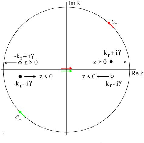
Figure 1: Schematic representation of the two symmetric poles $k_{r}+i\gamma$ and $-k_{r}-i\gamma$ by closed circles and two symmetric poles $-k_{r}+i\gamma$ and $k_{r}-i\gamma$ by open circles in the complex $k$ plane. Horizontal arrows near the poles show the wave direction. Also shown are two closed integration contours $\mathcal{C}_{+}$ for $z>0$ and $\mathcal{C}_{-}$ for $z<0$ of the residue method.

the determinant $\mbox{D}(c,\mathcal{K})$ is an even function of $c$. As shown in Fig. 1, one then obtains, through the relation (17), four poles in the complex $k$ plane

$$k_{0}=\pm k_{r}\pm i\gamma\leavevmode\nobreak\ ,$$ (22)

where $k_{r}$ and $\gamma$ are the absolute values of the sound-wave number and the absorption coefficient, respectively,

$$k_{r}\leavevmode\nobreak\ =\leavevmode\nobreak\ \frac{\omega}{v_{T}}\leavevmode\nobreak\ \frac{|c_{r}|}{c_{r}^{2}+c_{i}^{2}}\;,\leavevmode\nobreak\ \leavevmode\nobreak\ \leavevmode\nobreak\ \leavevmode\nobreak\ \leavevmode\nobreak\ \leavevmode\nobreak\ \frac{\gamma}{k_{r}}\leavevmode\nobreak\ =\leavevmode\nobreak\ \Big{|}\frac{c_{i}}{c_{r}}\Big{|}\leavevmode\nobreak\ .$$ (23)

The poles $k_{r}+i\gamma$ and $-k_{r}-i\gamma$ are related to the plane waves moving in the positive direction of the $z$ axis while $-k_{r}+i\gamma$ and $k_{r}-i\gamma$ correspond to the sound waves spreading in the negative $z$ direction (see Fig. 1). Taking, for example, $z>0$, one can close the integration path along the real axis of the complex $k$ plane in Eqs. (14) and (15) by adding the integration contour over the semicircle of a large radius in the upper half of this plane. The integrand along such a semicircle decreases exponentially with increasing the radius to infinity. This integration in Eqs. (14) and (15) can be performed by the residue method. As the result, one arrives at the APSW particle density [Eq. (14)] and velocity field [Eq. (15)], which are related to one of the poles $k_{0}=k_{r}+i\gamma$ [Eqs. (22) and (23)] for waves moving in the positive direction,

$$\delta n(z,t) \!=\! \!\left(\frac{\alpha_{k}V_{k}}{\mbox{d}\mbox{D}/\mbox{d}k}\right)_{k=k_{0}}\!\!\!\exp\left[-i\left(\omega t-k_{r}z\right)-\gamma z\right],\leavevmode\nobreak\ \leavevmode\nobreak\ \leavevmode\nobreak\$$

$$\delta u_{z}(z,t) \!=\! \!\left(\frac{\beta_{k}V_{k}}{\mbox{d}\mbox{D}/\mbox{d}k}\right)_{k=k_{0}}\!\!\!\exp\left[-i\left(\omega t-k_{r}z\right)-\gamma z\right].\leavevmode\nobreak\ \leavevmode\nobreak\ \leavevmode\nobreak\$$ (24)

Thus, one obtains the wave number $k_{r}>0$ and the absorption coefficient $\gamma>0$ for sound waves spreading in the positive $z$ axis direction for $z>0$. Similarly, one finds the contributions of other poles.

Let us consider the FCR where $\mathcal{K}\ll 1$. Taking the asymptotic expansion of $\mbox{D}(c,\mathcal{K})$ [Eq. (34)] in a series over $\mathcal{K}$, one finds (see Appendix B)

$$c_{r} \cong \sqrt{\frac{8}{9\pi}}+a_{2}(\omega\tau)^{2}+O\left((\omega\tau)^{4}\right)\leavevmode\nobreak\ ,$$

$$\frac{\gamma}{k_{r}} \cong \frac{21\pi-40}{40}\,\omega\tau+O\left((\omega\tau)^{3}\right)\leavevmode\nobreak\ ,$$ (25)

where $a_{2}$ is a constant given by Eq. (B). In the RCR $\mathcal{K}\gg 1$, one obtains, from the asymptotic expansion of Eq. (21) in $1/\omega\tau$ (Appendix C),

$$c_{r} \cong 1\leavevmode\nobreak\ -\frac{1}{(\omega\tau)^{2}}+O\left((\omega\tau)^{-4}\right)\leavevmode\nobreak\ ,$$

$$\frac{\gamma}{k_{r}} \cong \frac{1}{\omega\tau}+O\left((\omega\tau)^{-4}\right)\leavevmode\nobreak\ .$$ (26)

For small values of $\mathcal{K}$, or $\mathcal{K}^{-1}$, the real part $c_{r}$ of $c$ is an even function of $\mathcal{K}$, or $\mathcal{K}^{-1}$, i.e., it is expanded in even powers, while its imaginary part $c_{i}$ is expanded in odd powers. We emphasize that the FCR (III) and RCR (III) limits were obtained for the same sound velocity $c_{r}$ and absorption coefficient $\gamma/k_{r}$ as obtained, within the LRT, by the numerical solving of the dispersion equation (21) with the function (34). Notice also that one can obtain terms of the expansion in powers of $\leavevmode\nobreak\ \omega\tau\leavevmode\nobreak\$ $\leavevmode\nobreak\ (1/\omega\tau)$ at all orders by using the perturbation FCR (RCR) expansion and applying the same standard method of indeterminate multipliers in derivations of both Appendixes B and C.

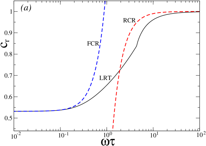
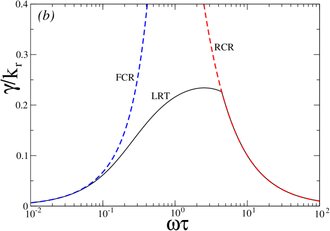
Figure 2: (a) Sound velocity $c_{r}$ in units of the thermal value $v_{T}$ and (b) scaled absorption coefficient $\gamma/k_{r}$ as functions of the Knudsen parameter $\omega\tau$. Solid lines show the nonperturbative LRT solutions. Dashed lines present the asymptotic FCR [Eq. (III)] and the RCR [Eq. (III)] approximations.

IV Discussion of the results

Figure 2 shows the sound velocity $c_{r}$ and scaled absorption coefficient $\gamma/k_{r}$ as functions of the Knudsen parameter $\omega\tau$. The results presented by solid lines are obtained by numerically solving the dispersion equation (21). The sound velocity $c_{r}$ is defined as a dimensionless quantity in units of $v_{T}$ given by Eq. (1). The quantity $v_{T}$ is the thermal particle velocity in a classical gas defined by the Maxwell distribution (5). Figure 2(a) demonstrates a nontrivial $\omega$ dependence of the sound velocity. In both limits $\omega\tau\ll 1$ and $\omega\tau\gg 1$, our numerical results converge to the asymptotic limits of the FCR and RCR, respectively. These limiting behaviors corresponding to Eqs. (III) and (III) at leading (quadratic) orders are shown by the dashed lines in this figure. Note that the sound velocity and scaled absorption coefficients are presented as universal functions of the Knudsen parameter $\omega\tau$ and, therefore, the lines in Fig.2 do not depend on the specific number coefficient in $\tau$ [Eq. (12)]. However, their $\omega$ behavior depends on this number coefficient such that the whole picture is shifted along the abscissa axis without changing the shapes of any lines.

The scaled absorption coefficient $\gamma/k_{r}$ measures how the amplitude of APSWs decreases after propagating a distance equal to the wavelength $\lambda$. The APSW amplitude decreases by the factor $e^{-1}$ with propagating the distance $\Delta z=1/\gamma$. In the FCR, for gases at normal conditions, one gets $\omega\tau\sim 10^{-8}--10^{-5}$ for the audible frequency region. This gives $\Delta z=1/\gamma_{\rm FC}\sim l(\omega\tau)^{-2}\sim 10^{5}--10^{11}$ cm. Thus, the audible sound wave propagates a distance of several kilometers without essential absorption in a gas. At the RCR for $\omega\tau\gg 1$, the behavior is quite different, $\Delta z=1/\gamma_{\rm RC}\sim l$, i.e., the propagating length is of the order of a mean free path. This quantity remains rather small even for dilute gases. Nevertheless, this regime is realized in experiments Gr65book ; Gr56 ; Me57 by using much larger ultrasonic frequencies and much smaller pressures (particle densities) of the gas. Note that these numbers in the FCR case are well known. We recall these known numbers to stress their great difference from those in the RCR. Very short propagation lengths of ultrasonic waves in gases are one of the problems for careful measurements of the absorption coefficient.

Figure 2(b) shows the scaled absorption coefficient $\gamma/k_{r}$ [Eq. (23)]. As can be seen from this figure, our numerical nonperturbative results for the scaled absorption coefficient shown by the solid line are in agreement with both the FCR (III) and the RCR (III) asymptotic limit presented by dashed lines. The absorption coefficient $\gamma/k_{r}$ as a function of the Knudsen parameter demonstrates a maximum at $\omega\tau\approx 1$ in the transition from the FCR to the RCR.

The kink in the dependence of the scaled absorption coefficient $\gamma/k_{r}$ and of the sound velocity $c_{r}$ on the Knudsen parameter is found at $\omega\tau\approx 4.4$, where the derivatives with respect to $\omega\tau$ are sharply changed. This is obtained in the numerical calculations, which are carefully checked within two different numerical schemes. There are two length scales in the problem: the mean free path of particles in a gas $l=v_{T}\tau$ and the sound wavelength $\lambda=c_{r}v_{T}2\pi/\omega$. The kink corresponds to the $\omega\tau$ point where these two different scales become approximately equal, $l\approx\lambda$. The presence of the kink cannot be proved as a mathematical theorem. It takes place in the nonperturbative region of $\omega\tau$ values, where no analytical solutions can be obtained. This resembles a situation similar to phase transitions in statistical mechanics. The origin of the kink remains an open problem that deserves further studies.

V Summary

The kinetic approach for calculations of the velocity and absorption coefficient for the absorbed plane sound waves is developed by solving the linearized Boltzmann kinetic equation with a small external plane-wave perturbation potential. The solution is based on the relaxation time approximation to the Boltzmann collision integral term for classical dilute gases. It was explicitly demonstrated that the mean particle density and velocity responses of the system, $\delta n$ and $\delta u_{z}$, to a small external potential $V_{\rm ext}$ determine the distribution function response $\delta f$ within the linear response theory. We obtained also explicitly the sound excitations of the particle density $\delta n(z,t)$ and velocity field $\delta u_{z}(z,t)$ in terms of the collective poles of the dispersion equation and found their structure.

The nonperturbative numerical solution to this equation is found for the sound velocity and absorption coefficient as functions of the Knudsen parameter $\omega\tau$ beyond both the frequent-collision and rare-collision regime approximations. This numerical solution agrees with the asymptotic expansions in both FCR and RCR. We found a dramatic change of the scaled absorption coefficient in the transition region between the frequent-collision and rare-collision regimes: a maximum of $\gamma/k_{r}$ at $\omega\tau\approx 1$.

The RCR in the kinetic theory is a subject that is not restricted only to the ultrasonic waves in classical gases. A strong difference between the FCR and RCR for sound waves means that the shear viscosity behaves very differently in these two regimes (see the discussion of this point in Ref. [35]). Other kinetic coefficients, i.e., the thermal conductivity and the diffusion coefficient, should also behave in a different way for the FCR and RCR.

One possible application of the kinetic theory in the RCR is high-energy nucleus-nucleus collisions. The intermediate stage of these collisions is often described by the hydrodynamical approach. The hydrodynamic description should be stopped at some stage (the so-called freeze-out procedure). After such a stage the system is usually considered as that of freestreaming particles. At this post-freeze-out stage, however, the particle collisions still occur and final momentum spectra are influenced by these collisions. This stage is the RCR of the kinetic models. The mean free path of particles flying away becomes larger than the system size.

Appendix A Method of the linear response

Using the linearization procedure in Eq. (I) and Fourier transformations (13)–(15), one has

$$\delta n_{k} = \int\mbox{d}{\bf p}\;\delta f_{k}({\bf p})\equiv\mathcal{D}_{k}\;V_{k}\;,$$

$$\delta u_{zk} = \frac{1}{mn}\int\mbox{d}{\bf p}\;p_{z}\delta f_{k}({\bf p})\equiv\mathcal{U}_{k}\;V_{k}\;,$$ (27)

where $\mathcal{D}_{k}$ and $\mathcal{U}_{k}$ are the corresponding response functions kubo ; zubarev ; hofmann ; baympeth ; heipethrav ; magkohofsh ; review . Substituting Eq. (A) into Eq. (16), one can represent it in the explicit form of the integral equation for $\delta f_{k}({\bf p})$:

$$\delta f_{k}({\bf p}) = \frac{if_{\rm GE}(p)}{\xi-\hat{p}_{z}}\;\left[\frac{c}{\mathcal{K}}\,\left(\frac{1}{n}\,\int\mbox{d}{\bf p}^{\prime}\leavevmode\nobreak\ \delta f_{k}({\bf p}^{\prime})\right.\right.$$ (28)

$$+ \left.\left.\frac{p_{z}}{mnT}\;\int\mbox{d}{\bf p}^{\prime}\;p_{z}^{\prime}\leavevmode\nobreak\ \delta f_{k}({\bf p}^{\prime})\right)-i\,\frac{\hat{p}_{z}}{T}\;V_{k}\,\right]\;.$$

This equation can be solved in terms of the response functions $\mathcal{D}_{k}$ and $\mathcal{U}_{k}$ [Eq. (A)]. From Eq. (18) with the help of Eq. (16), one gets the two linear equations

$$A_{1}\,\mathcal{D}_{k}+B_{1}\,\mathcal{U}_{k}=C_{1}\leavevmode\nobreak\ ,$$ (29)

$$A_{2}\,\mathcal{D}_{k}+B_{2}\,\mathcal{U}_{k}=C_{2}\,\leavevmode\nobreak\ ,$$ (30)

where

$$A_{1} = \left[i\,c\left(Q_{1}+1\right)/\left(\mathcal{K}\xi\right)-1\right]/n\leavevmode\nobreak\ ,$$

$$B_{1} = 4i\,c\,Q_{1}/\left(\sqrt{\pi}\leavevmode\nobreak\ \mathcal{K}\leavevmode\nobreak\ v_{T}\right)\leavevmode\nobreak\ ,$$

$$C_{1} = -Q_{1}/T\leavevmode\nobreak\ ,$$

$$A_{2} = 2i\,c\leavevmode\nobreak\ Q_{1}/\left(\sqrt{\pi}\leavevmode\nobreak\ \mathcal{K}\leavevmode\nobreak\ n\right)\leavevmode\nobreak\ ,$$

$$B_{2} = \left(3i\xi\,cQ_{1}/\mathcal{K}-1\right)/v_{T}\leavevmode\nobreak\ ,$$

$$C_{2} = -2\xi Q_{1}/\left(\sqrt{\pi}\leavevmode\nobreak\ T\right)\leavevmode\nobreak\ ,$$ (31)

and $Q_{1}$ is the Legendre function of second kind,

$$Q_{1}(\xi)\leavevmode\nobreak\ =\leavevmode\nobreak\ \frac{\xi}{2}\,\ln\left(\frac{\xi+1}{\xi-1}\right)\leavevmode\nobreak\ -\leavevmode\nobreak\ 1\leavevmode\nobreak\ .$$ (32)

Solving Eqs. (29) and (30), one obtains

$$\mathcal{D}_{k} = \frac{B_{2}C_{1}-B_{1}C_{2}}{\mbox{D}}\equiv\frac{\alpha_{k}}{\mbox{D}}\,\leavevmode\nobreak\ ,$$

$$\mathcal{U}_{k} = \frac{A_{1}C_{2}-A_{2}C_{1}}{\mbox{D}}\equiv\frac{\beta_{k}}{\mbox{D}}\,\leavevmode\nobreak\ ,$$ (33)

where D is the main determinant of the linear system of Eqs. (29) and (30),

D $$= \mbox{D}(c,\mathcal{K})=A_{1}B_{2}-A_{2}B_{1}$$ (34)

$$= \frac{1}{nv_{T}}\left\{\left[\frac{i\,c}{\xi\,\mathcal{K}}\;\left(1+Q_{1}\right)-1\right]\left(3i\,\frac{c}{\mathcal{K}}\,\xi\,Q_{1}-1\right)\right.$$

$$+ \left.\frac{8}{\pi}\;\left(\frac{c\,Q_{1}}{\mathcal{K}}\right)^{2}\right\}.$$

Substituting Eq. (A) into Eq. (16) with definitions (A), one arrives at the final solution (19) in terms of the response functions $\mathcal{D}_{k}$ and $\mathcal{U}_{k}$ with their explicit expressions (A).

Appendix B FCR derivations

By using the universal method of indeterminate coefficients brooksyk in the case of the FCR perturbation expansion over small $\mathcal{K}$,

$$c=a_{0}+a_{1}\leavevmode\nobreak\ \mathcal{K}+a_{2}\leavevmode\nobreak\ \mathcal{K}^{2}+a_{3}\leavevmode\nobreak\ \mathcal{K}^{3}+a_{4}\leavevmode\nobreak\ \mathcal{K}^{4}+\cdot\cdot\cdot\leavevmode\nobreak\ ,$$ (35)

one can solve the dispersion equation (21) with Eq. (34) for the determinant D. Substituting this perturbation series into the expansion of the function $\mbox{D}(c,\mathcal{K})$ [Eq. (34)] over $\mathcal{K}$ at a given $c$ (multiplied by a nonzero factor, e.g., $c^{6}/\mathcal{K}^{2}$ at the $\mathcal{K}^{4}$ order), one obtains the series that is an identity in powers of $\mathcal{K}$. Equaling the coefficients of this series at each power of $\mathcal{K}$, one arrives at the system of equations for the coefficients $a_{n}$ ($n=0,1,2,\ldots$):

$$a^{2}_{0}-\frac{8}{9\pi}=0\;,$$ (36)

$$\left(135\pi\leavevmode\nobreak\ a_{0}^{2}-80\right)a_{1}+45\leavevmode\nobreak\ i\pi\leavevmode\nobreak\ a_{0}^{3}+i(21\pi-80)a_{0}=0\;,$$ (37)

$$10\left(27\pi\leavevmode\nobreak\ a^{2}_{0}-16\right)a_{0}a_{2}+4i\left(135\pi\leavevmode\nobreak\ a^{2}_{0}+42\pi-160\right)a_{0}a_{1}$$

$$+\left(675\pi\leavevmode\nobreak\ a^{2}_{0}-240\right)a^{2}_{1}-\left(135\pi\leavevmode\nobreak\ a^{2}_{0}+168\pi-400\right)a^{2}_{0}$$

$$+48-9\pi=0\;,$$ (38)

and so on. We omitted common coefficients proportional to positive integer powers of $a_{0}$ to get the nonzero solutions. Solving consequently these equations step by step (for nonzero solutions), one obtains all coefficients.

For instance, at fourth-order terms, one obtains the polynomial equation of the sixth order with respect to $c$. Therefore, one finds three pairs of analytical solutions $c_{n}$, $n=1,2,\ldots,6$, namely $c_{2}=-c_{1}$, $c_{4}=-c_{3}$, and $c_{6}=-c_{5}$. The solutions of three roots, $a_{1}$, $a_{3}$ and $a_{5}$ can be presented by the Cardan formulas. For definiteness, taking the roots related to the positive solution for $a_{0}$ of Eq. (36), from Eqs. (36)–(B) one obtains

$$a_{0} = \sqrt{\frac{8}{9\pi}}\;,\qquad a_{1}=i\frac{40-21\pi}{30\sqrt{2\pi}}\;,\leavevmode\nobreak\ \leavevmode\nobreak\$$

$$a_{2} = \frac{423\pi^{2}-240\pi-1600}{1200\sqrt{2\pi}}\;,\leavevmode\nobreak\ \leavevmode\nobreak\$$

$$a_{3} = i\frac{30429\pi^{3}-44910\pi^{2}-16800\pi-112000}{84000\sqrt{2\pi}},\leavevmode\nobreak\ \leavevmode\nobreak\$$ (39)

and so on. Two other roots $c_{3}$ and $c_{5}$ are expansions over powers of $\mathcal{K}$ starting from the first-order term, which is proportional to $\mathcal{K}$. They are complex conjugated, $c_{5}=c^{\ast}_{3}$. For our purpose of the APSW description we have to select the root $c_{1}$ of the dispersion equation with a finite constant in the limit $\mathcal{K}\rightarrow 0$ as the physical solution.

The real part $c_{r}$ of the complex roots of Eq. (35) is expanded in even powers of $\mathcal{K}$ while its imaginary part $c_{i}$ is an expansion in odd powers of $\mathcal{K}$. Splitting Eq. (35) with found coefficients $a_{n}$ [Eq. (B)] into the real $c_{r}$ and imaginary $c_{i}$ parts of $c$, one finds

$$c_{r}(\mathcal{K}) = a_{0}+a_{2}\mathcal{K}^{2}+O\left(\mathcal{K}^{4}\right)\;,$$

$$c_{i}(\mathcal{K}) = a_{1}\mathcal{K}+a_{3}\mathcal{K}^{3}+O\left(\mathcal{K}^{5}\right)\;.$$ (40)

Therefore, according to Eq. (23), for the scaled absorption coefficient $\gamma/k_{r}$, one obtains the following FCR result up to fifth order terms:

$$\frac{\gamma}{k_{r}}=\frac{21\pi-40}{40}\;\mathcal{K}+q_{3}\mathcal{K}^{3}+O(\mathcal{K}^{5})\;,$$ (41)

where $q_{3}$ is an analytically given (rather bulky) number $q_{3}=-3.73421\ldots\leavevmode\nobreak\$ . Using Eqs. (B) and (41), one finally arrives at the main terms of Eq. (III).

Appendix C RCR derivations

In the RCR case, let us start with the perturbation expansion of solutions of the dispersion equation (21) with Eq. (34) for the determinant function $\mbox{D}(c,\mathcal{K})$ over a small Knudsen parameter $1/\mathcal{K}$,

$$c=a_{0}+a_{1}/\mathcal{K}+a_{2}/\mathcal{K}^{2}+a_{3}/\mathcal{K}^{3}+a_{4}/\mathcal{K}^{4}+\cdot\cdot\cdot\leavevmode\nobreak\ ,$$ (42)

where $a_{n}$ are new indeterminate coefficients. For simplicity of the presentation, up to third-order terms of the expansion of $\mbox{D}(c,\mathcal{K})$ over $1/\mathcal{K}$, one obtains

$$nv_{T}\mbox{D}(c,\mathcal{K})=1-\frac{ic}{2\mathcal{K}}\;\left[-6c+(1+3c^{2})\ln\left(\frac{c+1}{c-1}\right)\right]$$

$$-\frac{c^{2}}{4(c^{2}-1)\pi\mathcal{K}^{2}}\left\{8\left[4-\pi+c^{2}(3\pi-4)\right]\right.$$

$$-\left.2c(c^{2}-1)(9\pi-16)\leavevmode\nobreak\ \ln\left(\frac{c+1}{c-1}\right)\right.$$

$$+\left.c^{2}(c^{2}-1)(3\pi-8)\leavevmode\nobreak\ \ln^{2}\left(\frac{c+1}{c-1}\right)\right\}+\mbox{O}\left(\frac{1}{\mathcal{K}^{3}}\right)\;.$$ (43)

Substituting the expansion (42) with unknown coefficients $a_{n}$ ($n=0,1,\ldots,$) into the dispersion equation (21) with Eq. (C) for D and setting zero the expressions at any given order in $1/\mathcal{K}$ of the obtained identity, one finds the nonlinear system of equations with respect to these constants $a_{n}$. Starting from the linear approximation in $1/\mathcal{K}$, one obtains

$$\mbox{D}_{1}(a_{0},\mathcal{K})\equiv 1-ia_{0}/(2\mathcal{K})\;$$

$$\times\left[(1+3a^{2}_{0})\ln\left(\frac{a_{0}+1}{a_{0}-1}\right)-6a_{0}\right]=0\;.$$ (44)

At the second order, one finds the equation for $a_{1}$ as function of $a_{0}$,

$$\mbox{D}_{2}(a_{0},a_{1})\equiv 4a_{0}\left[2a_{0}(4-\pi)+a^{3}_{0}(6\pi-8)\right.$$

$$+i\left.\pi\leavevmode\nobreak\ a_{1}(5-9a^{2}_{0})\right]-2(a^{2}_{0}-1)\left[a^{3}_{0}(9\pi-16)\right.$$

$$-\left.i\pi\left(1+9a^{2}_{0}\right)a_{1}\right]\ln\left(\frac{a_{0}+1}{a_{0}-1}\right)$$

$$+a^{4}_{0}(a^{2}_{0}-1)(3\pi-8)\ln^{2}\left(\frac{a_{0}+1}{a_{0}-1}\right)=0\;,$$ (45)

and so on. The next equation having the structure $\mbox{D}_{3}(a_{0},a_{1},a_{2})=0\leavevmode\nobreak\$ gives $a_{2}$ as function of $a_{0}$ and $a_{1}$. Eq. (C) is a transcendent equation for only one variable $a_{0}$. Any given $n$th equation of this system $D_{n}(a_{0},a_{1},...,a_{n-1})=0$ is linear with respect to the last argument $a_{n-1}$. The last coefficient $a_{n-1}$ can easy be found analytically, as a function of all other (with smaller subscripts) variables. This determines the iteration perturbation procedure to obtain all of the coefficients $a_{n}$ in Eq. (42).

To get explicitly expansions for $a_{n}$ over $\mathcal{K}$, one notes that the solution of the first equation (C) with respect to $a_{0}$ converges asymptotically to one at $\mathcal{K}\to\infty$. Substituting this solution into expressions for $a_{n}$ ($n\geq 1$) in the remaining equations, one finally obtains the asymptotic series

$$c=\frac{\mathcal{K}}{i+\mathcal{K}}=1-\frac{i}{\mathcal{K}}-\frac{1}{\mathcal{K}^{2}}+\frac{i}{\mathcal{K}^{3}}+O\left(\frac{1}{\mathcal{K}^{4}}\right)\;.$$ (46)

The first two (linear) terms were obtained in Ref. MGGpre17 and are used here for the numerical calculations. Separating the real and imaginary parts from Eq. (46), one gets

$$c_{r} = 1-\frac{1}{\mathcal{K}^{2}}+O\left(\frac{1}{\mathcal{K}^{4}}\right)\;,$$

$$c_{i} = -\frac{1}{\mathcal{K}}+\frac{1}{\mathcal{K}^{3}}+O\left(\frac{1}{\mathcal{K}^{5}}\right)\;.$$ (47)

Thus, from this equation one finally arrives at Eq. (III).

References

- (1) L.D. Landau and E.M. Lifshitz, Hydrodynamics, Course of Theoretical Physics, (Nauka, Moscow, 2000), Vol. 6.
- (2) S. Chapman and T.G. Cowling, The Mathematical Theory of Non-Uniform Gases (Cambridge University Press. Cambridge, 1952).
- (3) M.N. Kogan, Dynamics of the Dilute Gas. Kinetic Theory, (Nauka, Fizmatlit, Moscow, 1967).
- (4) V.P. Silin, Introduction to the Kinetic Theory of Gases (Nauka, Moscow, 1971).
- (5) E.M. Lifshitz and L.P. Pitajevski, Physical Kinetics, Course of Theoretical Physics (Nauka, Moscow, 1981), Vol. 10.
- (6) Cercignani, The Boltzmann Equation and Its Application, (Springer, Berlin, 1988).
- (7) L.E. Reichl, A Modern Course in Statistical Physics, 2nd ed. (Wiley, New York, 1998).
- (8) M.I. Gorenstein, M. Hauer, and O.N. Moroz, Phys. Rev. C 77, 024911 (2008).
- (9) A.G. Magner, M.I. Gorenstein, U.V. Grygoriev, and V.A. Plujko, Phys. Rev. C 94, 054620 (2016).
- (10) A.A. Abrikosov and I.M. Khalatnikov, Rep. Prog. Phys. 22, 329 (1959).
- (11) M. Greenspan, in Physics Acoustics, edited by W.P. Mason (Academic, New York, 1965), Vol. II.
- (12) L. Sirovich and J. K. Thurber, J. Acoust Soc. Am. 37, 329 (1965).
- (13) E. P. Gross and E. A. Jackson, Phys. Fluids, 2, 432 (1959).
- (14) J. K. Buckner and J. H. Ferziger, Phys. Fluids, 9, 2315 (1966).
- (15) J. Sykes and G.A. Brooker, Ann. Phys. (N.Y.) 56, 1 (1970); G.A. Brooker and J. Sykes, ibid. 61, 387 (1970).
- (16) G. Lebon, Bull. Acad. Roy. Sci. Belgique 64, 45 (1978).
- (17) L.C. Woods, J. Fluid. Mech., 93, 585 (1979).
- (18) L.C. Woods and H. Troughton, J. Fluid. Mech., 100, 321 (1980).
- (19) S.R. de Groot, W.A. van Leeuwen, and C.G. van Weert, Relativistic Kinetic Theory, Principles and Applications (North-Holland, Amsterdam, 1980).
- (20) L.C. Woods, An Introduction to the Kinetic Theory of Gases and Magnetoplasmas (Oxford University Press, Oxford,1993).
- (21) G. Lebon and A. Cloot, Wave Motion, 11, 23 (1989).
- (22) N.G. Hadjiconstantinou and A.L. Garcia, Phys. of Fluids, 13, 1040 (2001).
- (23) X. Chen, H. Rao, and E.A. Spiegel, Phys. Lett. A 271, 87 (2000); Phys. Rev. E 64, 046309 (2001).
- (24) E.A. Spiegel and J.-L. Thiffeault, Phys. of Fluids, 15, 3558 (2003).
- (25) P. Massignan, G.M. Bruun, and H. Smith, Phys. Rev. A 71, 033607 (2005).
- (26) A. Wiranata and M. Prakash, Phys. Rev. C 85, 054908 (2012).
- (27) A. Wiranata, M. Prakash, and P. Chakraborty, Cent. Eur. J, Phys. 10, 1349 (2012).
- (28) N. Demir, A. Wiranata, J. Phys.: Conf. Ser. 535, 012018 (2014).
- (29) M. Albright and J.I. Kapusta, Phys. Rev. C 93, 014903 (2016).
- (30) K.F.Herzfeld, T.A. Litovitz, Absorption and Dispersion of Ultrasonic Waves (Academic, New York, 2013).
- (31) A.B. Bhatia, Ultrasonic Absorption: An Introduction to the Theory and Dispersion in Gases, Liquids and Solids (Dover, New York, 1985).
- (32) A.G. Magner, V.M. Kolomietz, H. Hofmann, and S. Shlomo, Phys. Rev. C 51, 2457 (1995).
- (33) V.M. Kolomietz, A.G. Magner, and S. Shlomo, Phys. Rev. C 73, 024312 (2006).
- (34) A.G. Magner, D.V. Gorpinchenko, and J. Bartel, Phys. At. Nucl., 77, 1229 (2014).
- (35) J.P. Blocki, A.G. Magner, and P. Ring, Phys. Rev. C 92, 064311 (2015).
- (36) C.J. Pethick and H. Smith, Bose-Einstein Condensation in Dilute Gases (Cambridge University Press, Cambridge, UK, 2002).
- (37) M. Greenspan, Phys. Rev. 75, 197 (1949); J. Acoust. Soc. Am. 22, 568 (1950).
- (38) M. Greenspan, J. Acoust. Soc. Am. 28, 644 (1956).
- (39) M.E. Meyer and G. Sessler, Z. Phys. 149, 15 (1957).
- (40) A.G. Magner, M.I. Gorenstein, and U.V. Grygoriev, Phys. Rev. E, 95, 052113 (2017).
- (41) R. Kubo, M. Toda, and N. Hashitsume, Statistical Physics II, Nonequilibrium Statistical Mechanics (Springer, New York, 1985).
- (42) D. Zubarev, V. Morozov, G. Röpke, Statistical Mechanics of Non-Equilibrium Processes (Fizmatlit, Moscow, 2002), Vol. II.
- (43) H. Hofmann, The Physics of Warm Nuclei with Analogies to Mesoscopic Systems (Oxford University Press, Oxford, 2008).
- (44) G. Baym and C.J. Pethick, Landau Fermi Liquid Theory (Wiley, New York, 1991).
- (45) H. Heiselberg, C.J. Pethick, and D.G. Revenhall, Ann. Phys. (N.Y.), 223, 37 (1993).