Compactly-Supported Smooth Interpolators for Shape Modeling with Varying Resolution

Abstract

In applications that involve interactive curve and surface modeling, the intuitive manipulation of shapes is crucial. For instance, user interaction is facilitated if a geometrical object can be manipulated through control points that interpolate the shape itself. Additionally, models for shape representation often need to provide local shape control and they need to be able to reproduce common shape primitives such as ellipsoids, spheres, cylinders, or tori. We present a general framework to construct families of compactly-supported interpolators that are piecewise-exponential polynomial. They can be designed to satisfy regularity constraints of any order and they enable one to build parametric deformable shape models by suitable linear combinations of interpolators. They allow to change the resolution of shapes based on the refinability of B-splines. We illustrate their use on examples to construct shape models that involve curves and surfaces with applications to interactive modeling and character design.

1 Introduction

The interactive modeling of curves and surfaces is desirable in applications that involve the visualization of shapes. Related domains include computer graphics [1, 2, 3, 4, 5, 6], image analysis in biomedical imaging [7, 8, 9, 10, 11], industrial shape design [12, 13, 14] or the modeling of animated surfaces [15]. Shape-modeling frameworks that allow for user interaction can usually be categorized in either discrete or continuous-domain models. Discrete models are typically based on interpolating polygon meshes or subdivision [16, 17, 18, 19, 20, 21] and they easily allow to locally refine a shape. Subdivision models are also considered as hybrids between discrete and continous-domain models because they iteratively define continuous functions in the limit. However, the limit functions do not always have a closed-form expression [22]. Continuous-domain models allow for organic shape modeling and consist of Bézier shapes or spline-based models such as NURBS [23, 24, 25]. They allow one to control shapes locally due to their compactly supported basis functions. However, NURBS generally cannot be smooth and interpolating at the same time, which leads to a non-intuitive manipulation of shapes because NURBS control points do not lie on the boundary of the object.

1.1 Motivation and Contribution

Our motivation is the practical need for interpolating functions to be used in user-interactive applications (see Figures 1 and 2). In this article, we present a general framework that combines the best of the discrete and continuous world: smooth and compactly supported basis functions, which are defined in the continuous domain satisfying the interpolation condition and allowing to vary the resolution of a constructed shape. In interactive shape modeling, these properties allow for the following key attributes:

• Organic shape modeling: smoothness enables a continuously-defined tangent plane and Gaussian curvature at any point on the surface, which facilitates realistic texturing and rendering of shapes;

• Local shape control: compact support combined with the interpolation property of the basis functions guarantees precise and direct shape interaction and an intuitive modeling process.

• Detailed surfacing: few parameters are required at the initial stage of modeling, while varying the resolution of the shape allows the user to increase the number of control points when more details are to be modeled.

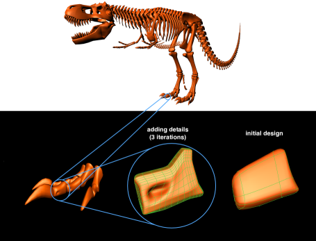
Figure 1: Interactive shape modeling for character design. Remodeling of the foot of the “T-rex” is shown. A bone of the middle toe of the right foot is modeled; first, an initial design is achieved with few control points that interpolate the shape (bottom, right). Then, the resolution is increased by applying three refinement iterations in order to have more flexibility to add details to the bone (bottom, middle). Due to convergence of our modified refinement scheme, after three iterations it behaves interpolatory-like.

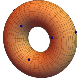
(a) Torus.

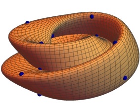
(b) “Figure 8” immersion.

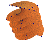
(c) Helicoid.

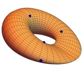
(d) Pinched torus.

Figure 2: Parametric surfaces constructed with the proposed family of interpolators. If the parameterization of a shape is known, we provide the formulae to construct the corresponding interpolator in order to represent the shape as detailed in Section 5. The interpolation property ensures that the control points (blue points) interpolate the surface. This property is particularly useful in user-interactive applications, where a surface is modified by dragging control points (e.g. as previously demonstrated in [26, 27])

Our framework consists of a new family of compactly supported interpolators that are linear combinations of shifted exponential B-splines on the half-integer grid. This allows us to harness useful properties of B-splines which are then transferred to the interpolators. We first derive general results and define the construction problem together with necessary constraints and conditions. We then establish relevant reproduction properties and show that, under suitable conditions, the integer shifts of the generators form a Riesz basis, which guarantees a unique and stable representation of the parametric shapes used in practice. The generators are compactly supported. Their degree of regularity can be increased at will. Based on extensive experimentations, we conjecture that the proposed construction always yields bona fide interpolators.

We further propose an algorithm to change the resolution of the generators which, in turn, allows us to change the resolution of the shapes. This demands that the generators be expressed as a linear combination of finer-resolution basis functions. For this purpose, we propose a refinement scheme associated to our generators by introducing a “pre-refinement” step such that the resulting refinement converges to the interpolator itself. In particular, we illustrate our theory by characterizing a family of symmetric and smooth interpolators that are at least in $\mathcal{C}^{1}$ and have compact support.

Finally, we present examples of applications that involve character design (Figure 1) as well as the design of idealized parametric shapes (Figure 2).

More specifically, Sections 3 and 4 are the main technical contributions, whereas in Section 5 we present practical applications which motivate this article.

1.2 Related Work

Recently, a method to build piecewise-polynomial interpolators has been presented in [28, 29] and its bivariate generalization was proposed in [30]. The present work is the continuation of our previous efforts to, first, generalize the popular Catmull-Rom [31] and Keys [32, 33] interpolators for practical applications [26, 27, 34, 35] and, next, to go one step further and construct families of interpolators that allow varying the resolution of a shape [36, 37]. Here, the novelty w.r.t. [35] is that the presented framework allows one to vary the resolution of shapes which facilitates shape design in practice, as illustrated in Section 5.2.1.

2 Review of Exponential B-Splines

We briefly review the link between exponential B-splines and differential operators. This is crucial to understand the properties of the proposed family of splines. For a more in-depth characterization of exponential B-splines, we refer the reader to [38].

2.1 Notation

We describe the list of roots associated to an exponential B-spline as $\bm{\alpha}=(\alpha_{1},\dots,\alpha_{n_{0}})$. Likewise, we write $\alpha_{n}\in\bm{\alpha}$ to signify that one of the components of $\bm{\alpha}$ is $\alpha_{n}$. The symbol $n_{d}$ refers to the number of distinct roots of $\bm{\alpha}$, which are denoted by $\alpha_{(1)},\dots,\alpha_{(n_{d})}$ with the multiplicity of $\alpha_{(m)}$ being $n_{(m)}$ and ${\sum_{m=1}^{n_{d}}n_{(m)}=n_{0}}$. The identity and derivative operators are denoted by $\mathrm{I}$ and $\mathrm{D}=\frac{\mathrm{d}}{\mathrm{d}t}$, respectively. We denote by $f(\cdot)$ a continuously defined function where the dot in parantheses represents the variable and by $a=(a[n])_{n\in\mathbb{Z}}$ a discrete sequence. The imaginary complex unit $\mathrm{i}$ satisfies $\mathrm{i}^{2}=-1$, while the Fourier integral of a function $f$ is denoted by $\widehat{f}(\omega)=\int_{\mathbb{R}}f(t)\mathrm{e}^{-\mathrm{i}\omega t}\mathrm{d}t$. Finally, the continuous convolutions between two functions $f$ and $g$ is defined by $(f\ast g)(t)=\int_{\mathbb{R}}f(t-u)g(u)\mathrm{d}u$, and the discrete convolution between two sequences $a$ and $b$, is defined by $(a\ast b)[k]=\sum\limits_{n=-\infty}^{+\infty}a[k-n]b[n]$, respectively. Furthermore, we use bold font to denote parametric shapes such as for example a 2D curve $\bm{r}(t)=(r_{x}(t),r_{y}(t))$.

2.2 Exponential B-Spline and the Reproduction of Exponential Polynomials

The exponential B-spline with parameter $\bm{\alpha}$ is defined in the Fourier domain as

$$\widehat{\beta}^{+}_{\bm{\alpha}}(\omega)=\prod\limits_{n=1}^{n_{0}}\frac{1-\mathrm{e}^{\alpha_{n}-\mathrm{i}\omega}}{\mathrm{i}\omega-\alpha_{n}}.$$ (1)

The function $\beta^{+}_{\bm{\alpha}}$ is compactly supported with support $[0,n_{0}]$ [38, Section III-A].

We denote by $\beta_{\bm{\alpha}}$ the corresponding centered (hence, non-causal) exponential B-spline, whose support is $[-n_{0}/2,n_{0}/2]$. We have therefore

$$\beta_{\bm{\alpha}}(t)=\beta^{+}_{\bm{\alpha}}(t+n_{0}/2),$$ (2)

with $\beta^{+}_{\bm{\alpha}}$ the causal B-spline defined in (1). The reason for introducing centered B-splines is that we shall define interpolators that are symmetric around the origin and, hence, centered.

It is well known that the exponential B-spline $\beta_{\bm{\alpha}}$ is intimately linked to the differential operator

$$\mathrm{L}_{\bm{\alpha}}=(\mathrm{D}-\alpha_{1}\mathrm{I})\ldots(\mathrm{D}-\alpha_{n_{0}}\mathrm{I}),$$ (3)

which implies that $\beta_{\bm{\alpha}}$ is able to reproduce the functions $p_{0}$ in the null space of $L_{\alpha}$ defined as $\mathrm{L}_{\alpha}p_{0}=0$. As a consequence, exponential B-splines can reproduce exponential polynomials that live in the space [38, Section III-C-2]

$${\mathrm{span}\{t^{n-1}\mathrm{e}^{\alpha_{(m)}t}\}_{m=1,\dots,n_{d};\ n=1,\dots,n_{(m)}}.}$$ (4)

3 General Characterization of the Interpolator

We consider generators that are constructed as a sum of half-integer shifted versions of a given exponential B-spline $\beta_{\bm{\alpha}}$.

Definition 1.

For a sequence $\lambda\in\ell_{1}(\mathbb{Z})$ and $\bm{\alpha}$ a vector of roots, we define

$$\phi_{\lambda,\bm{\alpha}}(t):=\sum_{n\in\mathbb{Z}}\lambda[n]\beta_{\bm{\alpha}}\left(t-\frac{n}{2}\right).$$ (5)

In the frequency domain, we then have

$$\widehat{\phi}_{\lambda,\bm{\alpha}}(\omega)=\left(\sum_{n\in\mathbb{Z}}\lambda[n]\mathrm{e}^{-\mathrm{i}\omega n/2}\right)\widehat{\beta}_{\bm{\alpha}}(\omega).$$ (6)

In what follows, we state the desired mathematical properties that the generator $\phi_{\lambda,\bm{\alpha}}$ should satisfy.

1. The generator $\phi_{\lambda,\bm{\alpha}}$ is interpolatory in the sense that, for any function $f\in\mathrm{span}\{\phi_{\lambda,\bm{\alpha}}(\cdot-k)\}_{k\in\mathbb{Z}}$, we have $f(t)=\sum_{k\in\mathbb{Z}}f[k]\phi_{\lambda,\bm{\alpha}}(t-k)$. This is equivalent to the interpolation condition

   $$\phi_{\lambda,\bm{\alpha}}(t)\big{|}_{t=k}=\delta[k]=\left\{\begin{aligned} 1&\mbox{ if }k=0\\ 0&\mbox{, otherwise}\\ \end{aligned}\right.,$$ (7)

   where $\delta[k]$ represents the Kronecker delta.

2. The generator $\phi_{\lambda,\bm{\alpha}}$ is compactly supported, which implies that the sequence $\lambda$ has a finite number of non-zero values.

3. The function $\phi_{\lambda,\bm{\alpha}}$ is smooth with at least a continuous derivative.

4. The family of the integer shifts of the generator $\{\phi_{\lambda,\bm{\alpha}}(\cdot-k)\}_{k\in\mathbb{Z}}$ forms a Riesz basis.

5. The generator $\phi_{\lambda,\bm{\alpha}}$ preserves the reproduction properties of the associated exponential B-spline $\beta_{\bm{\alpha}}$ in the sense that it is capable of reproducing the exponential polynomials in the null-space of the operator $\mathrm{L}_{\bm{\alpha}}$ defined in (3).

6. The generator $\phi_{\lambda,\bm{\alpha}}$ allows one to represent shapes at various resolutions.

We choose equispaced half-integer shifts of the exponential B-splines in Definition 1. The reason is that our problem has no solution using only integer shifts under Conditions I), II), and III): There is no smooth and compactly supported interpolator of the form $\sum_{k\in\mathbb{Z}}\lambda[k]\beta_{\bm{\alpha}}(t-k)$. This can easily be verified; for example, by plugging any polynomial B-spline into Definition 1 and using integer shifts while imposing the interpolation conditions: It turns out that there are not enough degrees of freedom to solve the problem due to the compact support of the B-splines as well as the smoothness condition, which forces the degree of the B-spline to be greater than $1$. Furthermore, by using half-integer shifts, we guarantee that our solution lives in the spline space of the next finer resolution; a property that can be exploited in practice, as detailed in Section 3.4.

3.1 Riesz Basis

We consider the space

$$V(\phi_{\lambda,\bm{\alpha}})=\left\{\sum_{n\in\mathbb{Z}}c[n]\phi_{\lambda,\bm{\alpha}}(\cdot-n),\ c\in\ell_{2}(\mathbb{Z})\right\}$$ (8)

of functions that is generated by the integer shifts of $\phi_{\lambda,\bm{\alpha}}$. Our requirement is that the family of functions $\{\phi_{\lambda,\bm{\alpha}}(\cdot-n)\}_{n\in\mathbb{Z}}$ forms a Riesz basis of $V(\phi_{\lambda,\bm{\alpha}})$, which ensures that the representation of a function in $V(\phi_{\lambda,\bm{\alpha}})$ is stable and unique. We show in this section that this is the case if $\{\beta_{\bm{\alpha}}(\cdot-n)\}_{n\in\mathbb{Z}}$ is itself a Riesz basis and if $\phi_{\lambda,\bm{\alpha}}$ is interpolatory.

Definition 2.

The family $\{\varphi_{n}\}_{n\in\mathbb{Z}}$ of functions forms a Riesz basis if

$$A\lVert c\rVert_{\ell_{2}(\mathbb{Z})}\leq\left\lVert\sum_{n\in\mathbb{Z}}c[n]\varphi_{n}\right\rVert_{L_{2}(\mathbb{R})}\leq B\lVert c\rVert_{\ell_{2}(\mathbb{Z})}$$ (9)

for some constants $A,B>0$ and any sequence $c=(c[n])_{n\in\mathbb{Z}}\in\ell_{2}(\mathbb{Z})$.

When $\varphi_{n}=\varphi(\cdot-n)$, (9) is equivalent to the Fourier-domain condition

$$A^{2}\leq\sum_{k\in\mathbb{Z}}\lvert\widehat{\varphi}(\omega-2k\pi)\rvert^{2}\leq B^{2}$$ (10)

for any $\omega\in\mathbb{R}$ [39]. The family $\{\beta_{\bm{\alpha}}(\cdot-n)\}_{n\in\mathbb{Z}}$ is a Riesz basis when $\bm{\alpha}$ is such that $\alpha_{n}-\alpha_{m}\neq 2k\pi\mathrm{i}$, $k\in\mathbb{Z}$, for any pair of distinct purely imaginary roots $\alpha_{m},\alpha_{n}\in\bm{\alpha}$ [38, Theorem 1].

Proposition 1.

Let $\bm{\alpha}$ be such that $\alpha_{n}-\alpha_{m}\neq 2k\pi\mathrm{i}$, $k\in\mathbb{Z}$, for any pair of distinct purely imaginary roots $\alpha_{m},\alpha_{n}\in\bm{\alpha}$. For any sequence $\lambda\in\ell_{1}(\mathbb{Z})$, if the basis function $\phi_{\lambda,\bm{\alpha}}$ is interpolatory, then the family $\{\phi_{\lambda,\bm{\alpha}}(\cdot-n)\}_{n\in\mathbb{Z}}$ is a Riesz basis.

The proof is given in A as well as an estimate of the Riesz Bounds.

3.2 Reproduction Properties

Proposition 2.

Let $\bm{\alpha}$ be a vector of roots. We assume that $\lambda\in\ell_{1}(\mathbb{Z})$ satisfies the conditions

$$\sum_{n\in\mathbb{Z}}\lvert\lambda[n]\rvert\mathrm{e}^{-\alpha n/2} <\infty,$$ (11)

$$\sum_{n\in\mathbb{Z}}\lambda[n]\mathrm{e}^{-\alpha n/2} \neq 0$$ (12)

for every $\alpha\in\bm{\alpha}$. Then, the basis function $\phi_{\lambda,\bm{\alpha}}$ has the same reproduction properties as the corresponding exponential B-spline $\beta_{\bm{\alpha}}$. In particular, it reproduces the exponential polynomials

$$t^{n-1}\mathrm{e}^{\alpha_{(m)}t}$$ (13)

for $m=1,\dots,n_{d}$ and $n=1,\dots,n_{(m)}$, with the notations of Section 2.1.

Note that (11) is always satisfied as soon as $\phi_{\lambda,\bm{\alpha}}$ is compactly supported. The proof of Proposition 2 is given in B.

3.3 Regularity

From Definition 1, it immediately follows that $\phi_{\lambda,\bm{\alpha}}$ has the same regularity as the exponential B-spline $\beta_{\bm{\alpha}}$ if $\lambda\neq 0$. Hence, $\phi_{\lambda,\bm{\alpha}}$ belongs to $\mathcal{C}^{n_{0}-2}$ [38, Section III-A].

3.4 Varying the Resolution of the Generator

The causal exponential B-spline $\beta_{\bm{\alpha}}^{+}$ is refinable, in the sense that its dilation by an integer $m$ can be expressed as a linear combination of $\beta_{\bm{\alpha}/m}^{+}(\cdot-k)$. This is what we refer to as the resolution of the basis function. We shall see how this property translates to the function $\phi_{\lambda,\bm{\alpha}}$. For this purpose, we first revisit the $m$-scale relation for exponential B-splines. For convenience, we express the corresponding terms with respect to causal (non-centered) B-splines. In practice, we always consider symmetric interpolators $\phi_{\lambda,\bm{\alpha}}$ with support $[-(n_{0}-1),n_{0}-1]$ (see Section 4). Therefore, we define the shifted and causal version of the interpolator as

$$\phi_{\lambda,\bm{\alpha}}^{+}(t)=\phi_{\lambda,\bm{\alpha}}(t-(n_{0}-1)).$$ (14)

Every causal formula is easily adapted to the centered case by applying a shift similar to (14). We follow the notations of [38], where an in-depth discussion on the refinability of exponential B-splines can be found.

As shown in [38, Section IV-D], the dilation by an integer $m\in\mathbb{N}\setminus\{0\}$ of an exponential B-spline is expressed in the space domain as

$$\beta^{+}_{\bm{\alpha}}\left(\frac{t}{m}\right)=\sum_{k\in\mathbb{Z}}h_{\frac{\bm{\alpha}}{m},m}[k]\beta^{+}_{\frac{\bm{\alpha}}{m}}(t-k),$$ (15)

where the refinement filter $h_{\bm{\alpha},m}$ is specified by its Fourier transform as

$$H_{\bm{\alpha},m}(\mathrm{e}^{\mathrm{i}\omega})=\frac{1}{m^{n_{0}-1}}\prod_{n=1}^{n_{0}}\bigg{(}\sum_{k=0}^{m-1}\mathrm{e}^{\alpha_{n}k}\mathrm{e}^{-\mathrm{i}k\omega}\bigg{)}.$$ (16)

As we shall see, it is impossible to establish a similar relation for the interpolator $\phi^{+}_{\lambda,\bm{\alpha}}$. However, we can exploit the refinability of the corresponding spline $\beta_{\bm{\alpha}}^{+}$ to express the dilation of $\phi^{+}_{\lambda,\bm{\alpha}}$.

For $\bm{\alpha}$ a vector of roots, $\lambda\in\ell_{1}(\mathbb{Z})$, and $m_{0}$ an even integer, we define the digital pre-filter $g_{\lambda,\bm{\alpha},m_{0}}$ by its Fourier transform

$$G_{\lambda,\bm{\alpha},m_{0}}(\mathrm{e}^{\mathrm{i}\omega})=\mathrm{e}^{-\mathrm{i}\omega m_{0}(n_{0}/2-1)}\left(\sum_{n\in\mathbb{Z}}\lambda[n]\mathrm{e}^{-\mathrm{i}\omega nm_{0}/2}\right)H_{\frac{\bm{\alpha}}{m_{0}},m_{0}}(\mathrm{e}^{\mathrm{i}\omega}).$$ (17)

The term $\mathrm{e}^{-\mathrm{i}\omega m_{0}(n_{0}/2-1)}$ is due to the fact that $\beta_{\bm{\alpha}}$ and $\phi_{\lambda,\bm{\alpha}}$ do not have the same support in general. The pre-filter allows us to express $\phi^{+}_{\lambda,\bm{\alpha}}$ dilated by $m_{0}$ as a linear combination of the refined shifted B-splines $\beta_{\frac{\bm{\alpha}}{m_{0}}}^{+}(\cdot-k)$. Note that $G_{\lambda,\bm{\alpha},m_{0}}$ is a valid Fourier transform of a digital filter (i.e., a function of $\mathrm{e}^{\mathrm{i}\omega}$) only for even $m_{0}$.

Proposition 3.

Let $\bm{\alpha}$ be a vector of roots, $\lambda\in\ell_{1}(\mathbb{Z})$, and $m_{0}$ be an even integer. Then, we have

$$\phi^{+}_{\lambda,\bm{\alpha}}\left(\frac{t}{m_{0}}\right)=\sum_{k\in\mathbb{Z}}g_{\lambda,\frac{\bm{\alpha}}{m_{0}},m_{0}}[k]\beta^{+}_{\frac{\bm{\alpha}}{m_{0}}}(t-k).$$ (18)

The proof is given in C.

3.4.1 Modified Refinement Scheme Based on Exponential B-Splines

Using Proposition 3, we are able to express a function which is constructed with the interpolator $\phi^{+}_{\lambda,\bm{\alpha}}$ in an exponential B-spline basis. Starting with the samples $c[k]=f(t)|_{t=k\in\mathbb{Z}}$ of a continuously defined function $f(\cdot)$ that can be perfectly reconstructed, i.e., $f\in\mathrm{span}\{\phi^{+}_{\lambda,\bm{\alpha}}(\cdot-k)\}_{k\in\mathbb{Z}}$, we have

$$f(t) =\sum_{k\in\mathbb{Z}}{c}[k]\phi^{+}_{\lambda,\bm{\alpha}}(t-k)$$

$$=\sum_{k\in\mathbb{Z}}{c}[k]\sum_{l\in\mathbb{Z}}g_{\lambda,\frac{\bm{\alpha}}{m_{0}},m_{0}}[l]\beta^{+}_{\frac{\bm{\alpha}}{m_{0}}}(m_{0}(t-k)-l)$$

$$=\sum_{k\in\mathbb{Z}}\sum_{l\in\mathbb{Z}}{c}[k]g_{\lambda,\frac{\bm{\alpha}}{m_{0}},m_{0}}[l]\beta^{+}_{\frac{\bm{\alpha}}{m_{0}}}(m_{0}t-m_{0}k-l)$$

$$=\sum_{l\in\mathbb{Z}}c_{0}[l]\beta^{+}_{\frac{\bm{\alpha}}{m_{0}}}(m_{0}t-l)$$ (19)

with

$$c_{0}[l]=\bigg{(}{c}_{\uparrow m_{0}}\ast g_{\lambda,\frac{\bm{\alpha}}{m_{0}},m_{0}}\bigg{)}[l],$$ (20)

where $\uparrow m_{0}$ denotes upsampling by a factor $m_{0}$ defined as

$${c_{\uparrow_{m_{0}}}[k]=\left\{\begin{array}[]{ll}c[n]\text{, }k=m_{0}n\\ 0\text{, otherwise.}\end{array}\right.}$$ (21)

Equation (3.4.1) shows that a function that is originally expressed in the basis generated by $\phi^{+}_{\lambda,\bm{\alpha}}$ can be expressed in a corresponding exponential B-spline basis with respect to a finer grid. This suggests that, after having performed the change of basis described by (3.4.1), the resolution of $f$ can be further refined by applying the standard iterative B-spline refinement rules. At this point, it is interesting to take a deeper look into the relation between the interpolated function $f$ and the sequence $c$ of samples as we iteratively refine it. As will become apparent in the application-oriented Section 5, a parametric shape is described by coordinate functions whose samples build 2D or 3D vectors of control points. Repositioning of these control points allows us to locally modify the shape, while the iterative refinement of the control points allows us to iteratively increase the local control over the shape. Hence, for practical purposes, it is convenient to study the convergence of the refinement process as the number of iterations becomes large. Proposition 4 describes the refinement scheme and provides the corresponding convergence result.

Proposition 4.

Let $\bm{\alpha}$ be a vector of roots and $\lambda\in\ell_{1}(\mathbb{Z})$. For a continuous function $f$ with samples $f(t)|_{t=k\in\mathbb{Z}}=c[k]$ and the integers $m,m_{0}$, with $m_{0}$ being even, we consider the iterative scheme specified by

1. pre-filter step: $c_{0}[k]=(g_{\lambda,\frac{\bm{\alpha}}{m_{0}},m_{0}}\ast{c}_{\uparrow m_{0}})[k]$;

2. iterative steps: for $n\geq 1$, $c_{n}[k]=(h_{\frac{\bm{\alpha}}{m_{0}m^{n}},m}\ast{(c_{n-1})}_{\uparrow m})[k]$,

where $\uparrow m$ denotes upsampling by a factor $m$ as defined in (21). Then, the iterative scheme is convergent, in the sense that

$$\lim_{n\rightarrow\infty}\sum_{k\in\mathbb{Z}}c_{n}[k]\delta\left(m_{0}m^{n}t-k\right)=f(t),$$ (22)

where $\delta$ is the Dirac distribution.

The proof is given in Appendix D.

3.4.2 Example

We illustrate how to refine the resolution of a circular pattern by applying Proposition 4. To efficiently take advantage of the interpolation property, we apply the “pre-refinement” step (20) at the first iteration. For the subsequent iterations, we apply the standard refinement given by (16) as described by Proposition 4. By doing so, we see that the iterative scheme converges towards the circle $\bm{r}(t)=\sum_{l\in\mathbb{Z}}{\bm{c}}_{0}[l]\beta^{+}_{\frac{\bm{\alpha}}{m_{0}}}(m_{0}t-l)=\sum_{k\in\mathbb{Z}}{\bm{r}}[k]\phi^{+}_{\bm{\alpha}}(t-k)$. The result of the algorithm is shown in Figure 3. In E, we provide the details on how to reconstruct the circle with our framework.

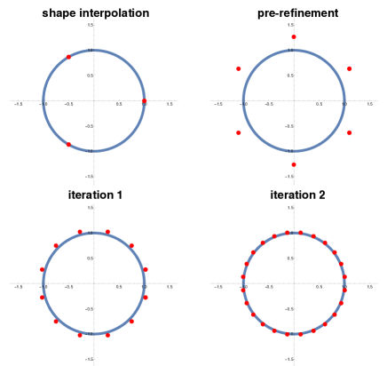
Figure 3: Refined circle. The parametric circle is first constructed using the proposed interpolator and $\bm{\alpha}=(0,\frac{2\mathrm{i}\pi}{3},-\frac{2\mathrm{i}\pi}{3})$ (top left). At the first iteration, the “pre-refinement” mask is applied to the initial control points according to (20) (top right), whereas at the subsequent iterations the standard refinement mask for exponential B-splines (16) is applied (bottom, from left to right). In the bottom right, we see how the iterative process converges towards the continuously defined circle.

4 Construction of a Family of Compactly Supported Interpolators in Practice

It is known that there exists no exponential B-spline $\beta_{\bm{\alpha}}$ that is interpolatory and smooth (i.e., at least in $\mathcal{C}^{1}$) at the same time. Our goal here is to construct a compactly supported generator function that has the same smoothness and reproduction properties as $\beta_{\bm{\alpha}}$, while also being interpolatory. In order to meet the smoothness constraints, we require the number of elements of $\bm{\alpha}$ to be $n_{0}\geq 3$ in accordance with the construction detailed in Section 3.3. Furthermore, we want the interpolator to be real-valued and symmetric, which implies that the elements of $\bm{\alpha}$ are either zero or come in complex conjugate pairs [38]. Using Definition 1 and the conditions described in Section 3, we are looking for the interpolator with minimal support.

4.1 Introductory Example: The Quadratic B-Spline

We illustrate the concept with a simple example that uses quadratic polynomial B-splines, which are constructed with $\bm{\alpha}=\bm{\alpha}_{0}=(0,0,0)$ in (1) and whose support is of size 3. The interpolation constraint combined with the half-integer shifts demand that $\lambda$ contains at least three non-zero values to have enough degrees of freedom. This also implies that the compactly-supported interpolator is constructed with no more than three non-zero elements of $\lambda$. Moreover, since the solution that fulfills the conditions stated in Section 3 is unique, the interpolator is of minimal support. To satisfy the symmetry constraints, we center the shifted B-splines around the origin and enforce $\lambda[1]=\lambda[-1]$. Hence, our generator must take the form

$$\begin{split}\phi_{\lambda,\bm{\alpha_{0}}}(t)&=\lambda[1]\beta_{\bm{\alpha_{0}}}(t-\frac{1}{2})+\lambda[0]\beta_{\bm{\alpha_{0}}}(t)+\lambda[-1]\beta_{\bm{\alpha_{0}}}(t+\frac{1}{2})\\ &=\lambda[0]\beta_{\bm{\alpha_{0}}}(t)+\lambda[1]\big{(}\beta_{\bm{\alpha_{0}}}(t-\frac{1}{2})+\beta_{\bm{\alpha_{0}}}(t+\frac{1}{2})\big{)}.\end{split}$$ (23)

Since $\bm{\alpha}_{0}$ has $n_{0}=3$ elements, the support of the interpolator is $N=2(n_{0}-1)=4$. The interpolator itself is supported in $[-(n_{0}-1),(n_{0}-1)]=[-2,2]$. The interpolation condition is expressed as $\begin{cases}\phi_{\lambda,\bm{\alpha_{0}}}(0)=1\\ \phi_{\lambda,\bm{\alpha_{0}}}(1)=0\end{cases}$. We define the matrix

$$\mathbf{A}_{\bm{\alpha}_{0}}=\begin{pmatrix}\beta_{\bm{\alpha_{0}}}(0)&\beta_{\bm{\alpha_{0}}}(-1/2)+\beta_{\bm{\alpha_{0}}}(1/2)\\ \beta_{\bm{\alpha_{0}}}(1)&\beta_{\bm{\alpha_{0}}}(1-1/2)+\beta_{\bm{\alpha_{0}}}(1+1/2)\end{pmatrix}=\left(\begin{array}[]{cc}\frac{3}{4}&1\\ \frac{1}{8}&\frac{1}{2}\\ \end{array}\right)$$

and rewrite the interpolation constraint as $(\lambda[0],\lambda[1])=\bm{\mathrm{A}}_{\bm{\alpha_{0}}}^{-1}(1,0)=(1,-\frac{1}{2})$. The resulting interpolator is shown in Figure 4.

4.2 The General Case

In what follows, we only consider vectors of poles $\bm{\alpha}$ for which $\alpha_{n}-\alpha_{m}\neq 2k\pi\mathrm{i}$, $k\in\mathbb{Z}$ for all pairs of distinct, purely imaginary roots $\alpha_{m},\alpha_{n}\in\bm{\alpha}$ (Riesz Basis property). We generalize the above example to construct symmetric and compactly supported interpolators of any order and that are of the form

$$\phi_{\lambda,\bm{\alpha}}(t):=\lambda[0]\beta_{\bm{\alpha}}(t)+\sum_{n=1}^{n_{0}-2}\lambda[n]\left(\beta_{\bm{\alpha}}(t-n/2)+\beta_{\bm{\alpha}}(t+n/2)\right),$$ (24)

whose support is included in $[-N/2,N/2]=[-(n_{0}-1),n_{0}-1]$. We easily pass from the general representation (5) to (24), adapted to the symmetric and compactly supported case, by setting $\lambda[n]=0$ when $\lvert n\rvert\geq n_{0}-1$ (support condition) and $\lambda[-n]=\lambda[n]$ for every $n$ (symmetry condition).

The function $\phi_{\lambda,\bm{\alpha}}$ is interpolatory if and only if

$$\phi_{\lambda,\bm{\alpha}}(0)=1\text{ and }\phi_{\lambda,\bm{\alpha}}(1)=\cdots=\phi_{\lambda,\bm{\alpha}}(n_{0}-2)=0.$$ (25)

This defines a linear system with $(n_{0}-1)$ unknown non-zero elements of $\lambda$, $\{\lambda[0],\ldots,\lambda[n_{0}-2]\}$, and $(n_{0}-1)$ equations. The system (25) has a solution if the matrix $\bm{\mathrm{A}}_{\bm{\alpha}}\in\mathbb{R}^{(n_{0}-1)\times(n_{0}-1)}$ defined for $k,l=0,\ldots,(n_{0}-2)$ by

$$[\bm{\mathrm{A}}_{\bm{\alpha}}]_{k+1,l+1}=\begin{cases}\beta_{\bm{\alpha}}(k)&\quad\text{if}\quad l=0\\ \beta_{\bm{\alpha}}(k-l/2)+\beta_{\bm{\alpha}}(k+l/2)&\quad\text{else}\end{cases}$$ (26)

is invertible. In this case, we have

$$\lambda=(\lambda[0],\ldots,\lambda[n_{0}-2])=\bm{\mathrm{A}}_{\bm{\alpha}}^{-1}(1,0,\ldots,0).$$ (27)

Knowing $\bm{\alpha}$, we can easily check if the matrix $\bm{\mathrm{A}}_{\bm{\alpha}}$ is invertible, which is the case for all the examples that we tested (we have already seen that it is true for $\bm{\alpha}=(0,0,0)$ is Section 4.1). From (27), we see that $\lambda$ is completely determined by $\bm{\alpha}$. This motivates Definition 3.

Definition 3.

Let $\bm{\alpha}$ be a vector of roots whose elements are either zero or come in pairs with opposite signs. If the matrix $\bm{\mathrm{A}}_{\bm{\alpha}}$ defined in (26) is invertible, then the interpolatory basis function $\phi_{\bm{\alpha}}$ is defined as

$$\phi_{\bm{\alpha}}:=\phi_{\lambda,\bm{\alpha}},$$ (28)

with $\lambda$ defined by (27).

We conjecture that the matrix $\bm{\mathrm{A}}_{\bm{\alpha}}$ is always invertible, and that we always can define an interpolator $\phi_{\bm{\alpha}}$ for any list of roots $\bm{\alpha}$. In the remaining of this article, we assume that $\bm{\mathrm{A}}_{\bm{\alpha}}$ is invertible and, therefore, that $\phi_{\bm{\alpha}}$ is well-defined. Under this assumption, the unicity of the vector $\lambda$ ensures that the interpolator $\phi_{\bm{\alpha}}$ in Definition 3 has minimal support among the interpolators of the form (5).

In practice, the type of interpolator that needs to be constructed depends on the parametric shape that is represented. For instance, for a rectangular surface, a polynomial interpolator is required and the vector $\bm{\alpha}$ of roots will have to consist of zeros. If instead we aim at representing circles, spheres, or ellipsoids (see Section 5), whose coordinate functions are trigonometric, we need to construct interpolators that preserve sinusoids. Therefore, $\bm{\alpha}$ will contain pairs of purely imaginary roots with opposite signs. Similarly, we can reproduce hyperbolic shapes by picking an $\bm{\alpha}$ that contains pairs of real roots with opposite signs. If an interpolator is required to reproduce both trigonometric and polynomial shapes, e.g., to construct a cylinder, then the corresponding polynomial and trigonometric root vectors are concatenated to construct $\bm{\alpha}$. Examples of different interpolators are shown in Figure 4.

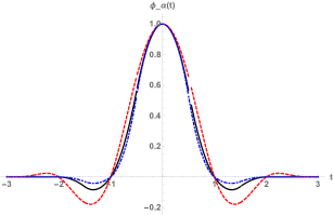
Figure 4: Different types of interpolators: polynomial interpolator (black, solid curve) with $\bm{\alpha}=(0,0,0)$. The number of poles is equal to $3$. Trigonometric interpolator (red, dashed curve): the non-zero poles are purely imaginary and come in pairs with opposite signs (e.g., $\bm{\alpha}=(0,0,\frac{\mathrm{i}2\pi}{3},-\frac{\mathrm{i}2\pi}{3})$). Hyperbolic interpolator (blue, dot-dashed curve): the non-zero poles are real and come in pairs with opposite signs (e.g., $\bm{\alpha}=(0,\frac{2\pi}{3},-\frac{2\pi}{3})$).

We now summarize the properties of the generator $\phi_{\bm{\alpha}}$ for $\bm{\alpha}$ a vector of roots of size $n_{0}\geq 3$ such that $\alpha_{n}-\alpha_{m}\neq 2k\pi\mathrm{i}$, $k\in\mathbb{Z}$, for any pair of distinct purely imaginary roots $\alpha_{m},\alpha_{n}\in\bm{\alpha}$ . These properties are in accordance with Conditions I to VI in Section 3.

• The function $\phi_{\bm{\alpha}}$ is interpolatory.

• The function $\phi_{\bm{\alpha}}$ is compactly supported in $[-(n_{0}-1),n_{0}-1]$.

• The function $\phi_{\bm{\alpha}}$ has the minimal support among the interpolators that are linear combinations of shifted exponential B-splines on the half-integer grid.

• The function $\phi_{\bm{\alpha}}$ is in $\mathcal{C}^{n_{0}-2}$ and therefore, at least in $\mathcal{C}^{1}$.

• The family $\{\phi_{\bm{\alpha}}(\cdot-n)\}_{n\in\mathbb{Z}}$ is a Riesz basis.

• The family $\{\phi_{\bm{\alpha}}(\cdot-n)\}_{n\in\mathbb{Z}}$ reproduces the exponential polynomials given by (4).

• The function $\phi_{\bm{\alpha}}$ is refinable in the sense explained in Section 3.4.

Remark. The presented interpolators are not (entirely) positive (see Figure 4) and thus, do not satisfy the convex-hull-property. However, the popularity of the Catmull-Rom splines [31] in computer graphics shows that in interactive shape modeling, one prefers to use interpolators at the expense of the convex-hull property.

5 Applications

In this section, we show how parametric curves and surfaces are constructed using the proposed spline bases. Such shapes can be constructed independently of the number of control points. This makes them particularly useful for deformable models where, starting from an initial configuration, one aims at approximating a target shape with arbitrary precision [39].

5.1 Reproduction of Idealized Shapes

We consider curves and surfaces that are described by the coordinate functions $r_{x}(t)$, $r_{y}(t)$, and $r_{z}(t)$, with $t\in\mathbb{R}$. The coordinate functions are expressed by a linear combination of weighted integer shifts of the generator $\phi_{\bm{\alpha}}$. Due to the interpolation property of the generator, the weights simply correspond to the samples of the coordinate functions. Such a parametric curve is expressed as

$$\bm{r}(t)=\begin{pmatrix}r_{x}(t)\\ r_{y}(t)\\ r_{z}(t)\end{pmatrix}=\sum_{k\in\mathbb{Z}}\bm{r}[k]\phi_{\bm{\alpha}}(t-k),$$ (29)

where the coefficients $\bm{r}[k]=(r_{x}[k],r_{y}[k],r_{z}[k])$ with $k\in\mathbb{Z}$ are the control points. The curve (29) can be locally modified by changing the position of a single control point. The shapes that $\bm{r}$ can adopt (e.g., polynomial, circular, elliptic) depend on the properties of the generator.

One can also extend the curve model (29) to represent separable tensor-product surfaces. In this case, a surface $\bm{\sigma}$ is parameterized by $u,v\in\mathbb{R}$ as

$$\begin{split}\bm{\sigma}(u,v)&=\begin{pmatrix}\bm{\sigma}_{x}(u,v)\\ \bm{\sigma}_{y}(u,v)\\ \bm{\sigma}_{z}(u,v)\end{pmatrix}=\begin{pmatrix}r_{1,x}(u)\cdot r_{2,x}(v)\\ r_{1,y}(u)\cdot r_{2,y}(v)\\ r_{1,z}(u)\cdot r_{2,z}(v)\\ \end{pmatrix}\\ &=\sum_{k\in\mathbb{Z}}\bm{r}_{1}[k]\phi_{\bm{\alpha}_{1}}(u-k)\times\sum_{l\in\mathbb{Z}}\bm{r}_{2}[l]\phi_{\bm{\alpha}_{2}}(v-l)\\ &=\sum_{k\in\mathbb{Z}}\sum_{l\in\mathbb{Z}}\underbrace{\bm{r}_{1}[k]\times\bm{r}_{2}[l]}_{\bm{\sigma}[k,l]}\phi_{\bm{\alpha}_{1}}(u-k)\phi_{\bm{\alpha}_{2}}(v-l),\end{split}$$ (30)

where “$\times$” denotes the element-wise multiplication of two vectors. Finally, one generalizes (30) to represent surfaces with a non-separable parameterization as

$$\bm{\sigma}(u,v)=\sum_{k\in\mathbb{Z}}\sum_{l\in\mathbb{Z}}\bm{\sigma}[k,l]\phi_{\bm{\alpha}_{1}}(u-k)\phi_{\bm{\alpha}_{2}}(v-l).$$ (31)

We use different families of interpolators to perfectly reproduce curves and surfaces with known parameterizations. In Section 5.1.1, we detail the construction of the Roman surface. Additional examples are provided in the appendices such as the reproduction of ellipses (E) and of the hyperbolic paraboloid (F). The four surfaces in Figure 2 were obtained from their classical parameterization following the same principle.

5.1.1 Reproduction of the Roman surface

An illustrative example is the Roman surface whose parametrization is

$$\bm{\sigma}(u,v) =\begin{pmatrix}\frac{1}{2}r^{2}\cos(2\pi u)\sin(4\pi v)\\ \frac{1}{2}r^{2}\sin(2\pi u)\sin(4\pi v)\\ r^{2}\cos(2\pi u)\sin(2\pi u)\cos^{2}(2\pi v)\end{pmatrix}$$ (32)

$$=\begin{pmatrix}\frac{1}{2}r^{2}\cos(2\pi u)\sin(4\pi v)\\ \frac{1}{2}r^{2}\sin(2\pi u)\sin(4\pi v)\\ \frac{1}{4}r^{2}\sin(4\pi u)(1+\cos(4\pi v)\end{pmatrix},\quad(u,v)\in\mathbb{R}^{2}.$$ (33)

We parameterize (32) as a tensor-product surface of the form (30) and denote by $M_{1}$ and $M_{2}$ the number of control points related to $\phi_{\bm{\alpha}_{1}}$ and $\phi_{\bm{\alpha}_{2}}$. The surface is trigonometric in $u$ and $v$. Hence, we choose to construct the interpolators $\phi_{\bm{\alpha}_{1}}$ and $\phi_{\bm{\alpha}_{2}}$ with $\bm{\alpha}_{1}=\left(\frac{2\mathrm{i}\pi}{M_{1}},\frac{-2\mathrm{i}\pi}{M_{1}},\frac{4\mathrm{i}\pi}{M_{1}},\frac{-4\mathrm{i}\pi}{M_{1}}\right)$ and $\bm{\alpha}_{2}=\left(0,\frac{4\mathrm{i}\pi}{M_{2}},\frac{-4\mathrm{i}\pi}{M_{2}}\right)$ to express (32) as

$$\bm{\sigma}(u,v)=\sum_{k\in\mathbb{Z}}\sum_{l\in\mathbb{Z}}\bm{\sigma}[k,l]\phi_{\bm{\alpha}_{1}}(M_{1}u-k)\phi_{\bm{\alpha}_{2}}(M_{2}v-l).$$ (34)

In order to satisfy the relation $\alpha_{n}-\alpha_{m}\neq 2k\pi\mathrm{i}$, $k\in\mathbb{Z}$ for all pairs of distinct, purely imaginary roots, we choose $M_{1}=M_{2}=5$. To construct $\phi_{\bm{\alpha}_{1}}$, we see that $n_{0}=4$ and $N=2(n_{0}-1)=6$. Hence, the support of $\phi_{\bm{\alpha}_{1}}$ is of size $6$. Following (24), the interpolator is expressed as

$$\phi_{\bm{\alpha}_{1}}(t)=\lambda[0]\beta_{\bm{\alpha}_{1}}(t)+\lambda[1]\bigg{(}\beta_{\bm{\alpha}_{1}}(t-\frac{1}{2})+\beta_{\bm{\alpha}_{1}}(t+\frac{1}{2})\bigg{)}+\lambda[2]\bigg{(}\beta_{\bm{\alpha}_{1}}(t-1)+\beta_{\bm{\alpha}_{1}}(t+1)\bigg{)}.$$

By solving the corresponding system of equations (25) for the non-zero entries of $\lambda$, we find $\lambda[0]=18.118$, $\lambda[1]=-10.128$, and $\lambda[2]=1.730$. For the construction of $\phi_{\bm{\alpha}_{2}}$, we have that $n_{0}=3$ and $N=2(n_{0}-1)=4$. The support of $\phi_{\bm{\alpha}_{2}}$ is therefore equal to $4$ and the interpolator is expressed as

$$\phi_{\bm{\alpha}_{2}}(t)=\lambda[0]\beta_{\bm{\alpha}_{2}}(t)+\lambda[1]\bigg{(}\beta_{\bm{\alpha}_{2}}(t-\frac{1}{2})+\beta_{\bm{\alpha}_{2}}(t+\frac{1}{2})\bigg{)}.$$

By solving (25), we find that $\lambda[0]=7.396$ and $\lambda[1]=-2.825$.

Since the generator is an interpolator, the control points of the surface are given by its samples, specified by

$$\bm{\sigma}(u,v)\big{|}_{u=k,v=l}=\begin{pmatrix}\frac{1}{2}r^{2}\cos(\frac{2\pi k}{M_{1}})\sin(\frac{4\pi l}{M_{2}})\\ \frac{1}{2}r^{2}\sin(\frac{2\pi k}{M_{1}})\sin(\frac{4\pi l}{M_{2}})\\ r^{2}\cos(\frac{2\pi k}{M_{1}})\sin(\frac{2\pi k}{M_{1}})\cos^{2}(\frac{2\pi l}{M_{2}})\end{pmatrix}.$$

We choose $(u,v)\in[0,1]^{2}$ and $r=3$. Then, the sums in (30) are finite due to the compact support of the generators. The parameterization of the surface is given by $\bm{\sigma}(u,v)=\sum\limits_{k=-2}^{M_{1}+2}\sum\limits_{l=-1}^{M_{2}+1}\bm{\sigma}[k,l]\phi_{\bm{\alpha}_{1}}(M_{1}u-k)\phi_{\bm{\alpha}_{2}}(M_{2}v-l).$ The Roman surface is illustrated in Figure 5.

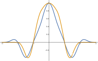
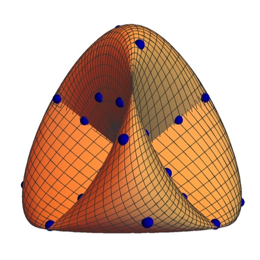
Figure 5: Roman surface. The interpolators $\phi_{\bm{\alpha}_{1}}$ (blue) and $\phi_{\bm{\alpha}_{2}}$ (yellow) are shown as well as the reconstructed surface (right). The interpolatory control points are shown as blue dots on the surface.

5.2 Interactive Shape Modeling

The presented interpolators are well suited to be implemented in an interactive shape modeling framework; for instance, for CAD design. The key properties in such a context are

• interpolation property: it allows to easily interact with the surface by displacing control points with a computer mouse;

• varying resolution: once the “rough” outline of the shape is designed, the details are modeled by increasing the resolution at specific locations.

5.2.1 Example: Character Design

The interpolation property is convenient to design complex shapes as shown in Figure 1 in order to obtain a low resolution model. To increase the level of detail of the shape, we increase the resolution of the surface by first applying the pre-refinement step (20) and then the standard refinement mask for (exponential) B-splines (16). These two steps increase the number of control points, however, at the expense of being interpolatory. This increase in the number of control points allows one to have more flexibility in the modeling process. Furthermore, after few iterations, the convergence of the proposed modified refinement scheme allows for an interpolatory-like behavior (see Figure 1).

6 Discussion and Conclusion

We have presented a general framework to construct interpolators as linear combinations of exponential B-splines of the same order $n_{0}$. The interpolators are compactly supported and their integer shifts form a Riesz basis whenever the corresponding B-spline does. Since the underlying building blocks are exponential B-splines, we can exploit the refinability property of the B-splines to resample the model. Based on these general properties, we have constructed a new family of interpolators to represent parametric shapes. The new interpolators are smooth and they can be designed to perfectly reproduce polynomial, trigonometric, and hyperbolic shapes. We provide explicit examples of such generators and show in detail how idealized parametric curves and surfaces are constructed. The reconstructed shapes have the property that the control points directly lie on their boundary. This enables an intuitive manipulation of shapes by changing the location of a control point. Since the interpolators have compact support, this displacement of control points allows one to locally control the deformation of a shape. In a next step, we plan to further investigate the refinability properties for practical applications such as real-time rendering or zooming of images.

7 Acknowledgements

This work was funded by the Swiss National Science Foundation under grant 200020-162343.

Appendix A Proof of Proposition 1

Proof.

We split the proof into two parts: the existence of an upper bound, relying on the one for the corresponding exponential B-spline, and the lower bound, based on the fact that the function is interpolatory.

Upper Bound

We first show that one can find $B_{\bm{\alpha}}<\infty$ such that, for every $\omega\in\mathbb{R}$,

$$\sum_{k\in\mathbb{Z}}\lvert\widehat{\beta}_{\bm{\alpha}}(\omega-2k\pi)\rvert^{2}\leq B_{\bm{\alpha}}^{2}.$$ (35)

This result is well-known (see for instance [38, Theorem 1]); we prove it for the sake of completeness. A more precise estimation of $B_{\bm{\alpha}}$ is given in [38, Proposition 3]. The function $\beta_{\bm{\alpha}}*\beta_{\bm{\alpha}}^{\vee}$, where $\beta_{\bm{\alpha}}^{\vee}(t)=\beta_{\bm{\alpha}}(-t)$, is continuous and compactly supported. Therefore, the sequence $c=(c[n])_{n\in\mathbb{Z}}=(\beta_{\bm{\alpha}}*\beta_{\bm{\alpha}}^{\vee}(n))_{n\in\mathbb{Z}}$ of its samples is in $\ell_{1}(\mathbb{Z})$. Since the Fourier transform of $\beta_{\bm{\alpha}}*\beta_{\bm{\alpha}}^{\vee}(t)$ is $\lvert\widehat{\beta}_{\bm{\alpha}}(\omega)\rvert^{2}$, we have that

$$\sum_{k\in\mathbb{Z}}\lvert\widehat{\beta}_{\bm{\alpha}}(\omega-2k\pi)\rvert^{2}=\sum_{k\in\mathbb{Z}}c[k]\mathrm{e}^{-\mathrm{i}\omega k}\leq\lVert c\rVert_{\ell_{1}(\mathbb{Z})}:=B_{\bm{\alpha}}^{2}<\infty.$$ (36)

Using (6), we moreover have that

$$\sum_{k\in\mathbb{Z}}\lvert\widehat{\phi}_{\lambda,\bm{\alpha}}(\omega-2k\pi)\rvert^{2}=\sum_{k\in\mathbb{Z}}\left(\sum_{n\in\mathbb{Z}}\lambda[n]\mathrm{e}^{-\mathrm{i}(\omega-2k\pi)n/2}\right)^{2}\lvert\widehat{\beta}_{\bm{\alpha}}(\omega-2k\pi)\rvert^{2}.$$ (37)

By splitting the sum with respect to $k$ odd or even and since $\mathrm{e}^{-\mathrm{i}(\omega-2k\pi)n/2}=((-1)^{k})^{n}\mathrm{e}^{-\mathrm{i}\omega n/2}$, we have that

$$\sum_{k\in\mathbb{Z}}\lvert\widehat{\phi}_{\lambda,\bm{\alpha}}(\omega-2k\pi)\rvert^{2}=|G_{0}(\omega)|^{2}\sum_{k\text{ even}}\lvert\widehat{\beta}_{\bm{\alpha}}(\omega-2k\pi)\rvert^{2}+|G_{1}(\omega)|^{2}\sum_{k\text{ odd}}\lvert\widehat{\beta}_{\bm{\alpha}}(\omega-2k\pi)\rvert^{2}$$ (38)

with $G_{0}(\omega)=\sum_{n\in\mathbb{Z}}\lambda[n]\mathrm{e}^{-\mathrm{i}\omega n/2}\text{ and }G_{1}(\omega)=\sum_{n\in\mathbb{Z}}(-1)^{n}\lambda[n]\mathrm{e}^{-\mathrm{i}\omega n/2}.$ Clearly, for $i=0,1$, $\lvert G_{i}(\omega)\rvert\leq\sum_{n\in\mathbb{Z}}|\lambda[n]\rvert=\lVert\lambda\rVert_{\ell_{1}(\mathbb{Z})}$ and thus,

$$\sum_{k\in\mathbb{Z}}\lvert\widehat{\phi}_{\lambda,\bm{\alpha}}(\omega-2k\pi)\rvert^{2} \leq\lVert\lambda\rVert_{\ell_{1}(\mathbb{Z})}^{2}\left(\sum_{k\text{ even}}\lvert\widehat{\beta}_{\bm{\alpha}}(\omega-2k\pi)\rvert^{2}+\sum_{k\text{ odd}}\lvert\widehat{\beta}_{\bm{\alpha}}(\omega-2k\pi)\rvert^{2}\right)$$

$$=\lVert\lambda\rVert_{\ell_{1}(\mathbb{Z})}^{2}\sum_{k\in\mathbb{Z}}\lvert\widehat{\beta}_{\bm{\alpha}}(\omega-2k\pi)\rvert^{2}$$

$$\leq\lVert\lambda\rVert_{\ell_{1}(\mathbb{Z})}^{2}B_{\bm{\alpha}}^{2},$$

so that the constant $B_{\lambda,\bm{\alpha}}=\lVert\lambda\rVert_{\ell_{1}(\mathbb{Z})}B_{\bm{\alpha}}<\infty$ acts as an upper bound in (10).

Lower Bound

The function $\phi_{\lambda,\bm{\alpha}}$ is assumed to be interpolatory; in the frequency domain, this condition is expressed as

$$\sum_{k\in\mathbb{Z}}\widehat{\phi}_{\lambda,\bm{\alpha}}(\omega-2k\pi)=1\quad\text{for all}\quad\omega\in\mathbb{R}.$$ (39)

Moreover, the functions $\omega\mapsto\sum_{k\in\mathbb{Z}}\lvert\widehat{\beta}_{\bm{\alpha}}(\omega-2k\pi)\rvert^{2}$, $G_{0}$, and $G_{1}$ above are also continuous and periodic (for $G_{0}$ and $G_{1}$, this comes from $\lambda\in\ell_{1}(\mathbb{Z})$). Therefore, the function $\omega\mapsto\sum_{k\in\mathbb{Z}}\lvert\widehat{\phi}_{\lambda,\bm{\alpha}}(\omega-2k\pi)\rvert^{2}$ is also continuous and periodic. As such, it reaches its minimum at some frequency $\omega_{0}\in[0,2\pi]$. Further, the inequality $A_{\lambda,\bm{\alpha}}^{2}:=\sum_{k\in\mathbb{Z}}\lvert\widehat{\phi}_{\lambda,\bm{\alpha}}(\omega_{0}-2k\pi)\rvert^{2}\geq 0$ holds. Assume now that $A_{\lambda,\bm{\alpha}}=0$, then we have $\widehat{\phi}_{\bm{\alpha}}(\omega_{0}-2k\pi)=0$ for every $k\in\mathbb{Z}$, and therefore, $\sum_{k\in\mathbb{Z}}\widehat{\phi}_{\lambda,\bm{\alpha}}(\omega_{0}-2k\pi)=0$, which contradicts (39). Hence, $A_{\lambda,\bm{\alpha}}>0$ acts as a lower bound in (10). ∎

Remark. Based on (38), we deduce the following estimates for the Riesz constants $A_{\lambda,\bm{\alpha}}$ and $B_{\lambda,\bm{\alpha}}$ associated to $\phi_{\lambda,\bm{\alpha}}$:

$$A_{\lambda,\bm{\alpha}} =A_{\bm{\alpha}}\min_{[0,2\pi]}\lvert\hat{\lambda}(\mathrm{e}^{\mathrm{i}\omega})\rvert,$$ (40)

$$B_{\lambda,\bm{\alpha}} =B_{\bm{\alpha}}\max_{[0,2\pi]}\lvert\hat{\lambda}(\mathrm{e}^{\mathrm{i}\omega})\rvert,$$ (41)

where $A_{\bm{\alpha}}$ and $B_{\bm{\alpha}}$ are the constants for the Riesz basis condition for $\beta_{\bm{\alpha}}$ (given in Proposition 4 and Proposition 3 in [38]), and $\hat{\lambda}(\mathrm{e}^{\mathrm{i}\omega})=\sum_{n\in\mathbb{Z}}\lambda[n]\mathrm{e}^{-\mathrm{i}\omega n/2}$ is the discrete Fourier transform of $\lambda$.

Appendix B Proof of Proposition 2

Proof.

The result follows from Proposition 2 in [38] which states that reproduction properties are preserved through convolution. More precisely, if $f$ is such that $\int_{-\infty}^{+\infty}f(t)\mathrm{e}^{-\alpha t}\mathrm{d}t\neq 0$ for all $\alpha\in\bm{\alpha}$, then $f*\beta_{\bm{\alpha}}$ inherits the reproduction properties of $\beta_{\bm{\alpha}}$. In our case, we have $\phi_{\lambda,\bm{\alpha}}(t)=(f*\beta_{\bm{\alpha}})(t)$ with $f(t)=\sum_{n\in\mathbb{Z}}\lambda[n]\delta(t-n/2)$. Then, for every $\alpha\in\bm{\alpha}$,

$$\int_{-\infty}^{+\infty}f(t)\mathrm{e}^{-\alpha t}\mathrm{d}t=\sum_{n\in\mathbb{Z}}\lambda[n]\mathrm{e}^{-\alpha n/2},$$ (42)

which is bounded and non-zero by assumption. ∎

Appendix C Proof of Proposition 3

Proof.

For the causal generator, we use (2) and (14) to express (6) as

$$\widehat{\phi}_{\lambda,\bm{\alpha}}^{+}(\omega)=\mathrm{e}^{-\mathrm{i}\omega(n_{0}/2-1)}\left(\sum_{n\in\mathbb{Z}}\lambda[n]\mathrm{e}^{-\mathrm{i}\omega n/2}\right)\widehat{\beta}_{\bm{\alpha}}^{+}(\omega).$$ (43)

Then, we have

$$m_{0}\widehat{\phi}_{\lambda,\bm{\alpha}}^{+}(m_{0}\omega) =\mathrm{e}^{-\mathrm{i}\omega m_{0}(n_{0}/2-1)}\left(\sum_{n\in\mathbb{Z}}\lambda[n]\mathrm{e}^{-\mathrm{i}m_{0}\omega n/2}\right)m_{0}\widehat{\beta}_{\bm{\alpha}}^{+}(m_{0}\omega)$$

$$=\mathrm{e}^{-\mathrm{i}\omega m_{0}(n_{0}/2-1)}\left(\sum_{n\in\mathbb{Z}}\lambda[n]\mathrm{e}^{-\mathrm{i}m_{0}\omega n/2}\right)H_{\frac{\bm{\alpha}}{m_{0}},m_{0}}(\mathrm{e}^{\mathrm{i}\omega})\widehat{\beta}_{\frac{\bm{\alpha}}{m_{0}}}^{+}(\omega)$$

$$=G_{\lambda,\frac{\bm{\alpha}}{m_{0}},m_{0}}(\mathrm{e}^{\mathrm{i}\omega})\widehat{\beta}_{\frac{\bm{\alpha}}{m_{0}}}^{+}(\omega),$$ (44)

where we used the relation (15) expressed in the frequency domain. Finally, we take the inverse Fourier transform of (C) and obtain (18) in the time domain. ∎

Appendix D Proof of Proposition 4

Proof.

Equation (22) is equivalent to the frequency domain relation

$$\lim_{n\rightarrow\infty}\frac{1}{m_{0}m^{n}}C_{n}(\mathrm{e}^{\frac{\mathrm{i}\omega}{m_{0}m^{n}}})=\widehat{f}(\omega),$$ (45)

where $C_{n}(z)=\sum_{k=-\infty}^{+\infty}c_{n}[k]z^{-k}$ is the $z$-transform of the discrete sequence $c_{n}=(c_{n}[k])_{k\in\mathbb{Z}}$. The iterative step between $c_{n}$ and $c_{n-1}$ in the frequency domain becomes

$$C_{n}(\mathrm{e}^{\frac{\mathrm{i}\omega}{m_{0}m^{n}}})=H_{\frac{\bm{\alpha}}{m_{0}m^{n}},m}(\mathrm{e}^{\frac{\mathrm{i}\omega}{m_{0}m^{n}}})C_{n-1}(\mathrm{e}^{\frac{\mathrm{i}\omega}{m_{0}m^{n-1}}}).$$ (46)

Iterating this relation, we obtain

$$C_{n}(\mathrm{e}^{\frac{\mathrm{i}\omega}{m_{0}m^{n}}})=\left(\prod_{k=1}^{n}H_{\frac{\bm{\alpha}}{m_{0}m^{k}},m}(\mathrm{e}^{\frac{\mathrm{i}\omega}{m_{0}m^{k}}})\right)C_{0}(\mathrm{e}^{\frac{\mathrm{i}\omega}{m_{0}}}).$$ (47)

By expressing (15) iteratively in the frequency domain and replacing $\bm{\alpha}$ by $\bm{\alpha}/m_{0}$, we see that

$$\begin{split}\widehat{\beta}_{\frac{\bm{\alpha}}{m_{0}}}^{+}(\omega)&=\frac{1}{m}H_{\frac{\bm{\alpha}}{m_{0}m},m}(\mathrm{e}^{\frac{\mathrm{i}\omega}{m}})\widehat{\beta}_{\frac{\bm{\alpha}}{m_{0}m}}^{+}\left(\frac{\omega}{m}\right)\\ &=\left(\prod_{k=1}^{n}\frac{1}{m}H_{\frac{\bm{\alpha}}{m_{0}m^{k}},m}(\mathrm{e}^{\frac{\mathrm{i}\omega}{m^{k}}})\right)\widehat{\beta}_{\frac{\bm{\alpha}}{m_{0}m^{n}}}^{+}\left(\frac{\omega}{m^{n}}\right)\\ &=\lim_{n\rightarrow\infty}\prod_{k=1}^{n}\frac{1}{m}H_{\frac{\bm{\alpha}}{m_{0}m^{k}},m}(\mathrm{e}^{\frac{\mathrm{i}\omega}{m^{k}}}),\end{split}$$ (48)

where in the last line we have used the well-known convergence result from spline theory [18, 40, 41]

$$\lim_{n\rightarrow\infty}\widehat{\beta}_{\frac{\bm{\alpha}}{m_{0}m^{n}}}^{+}\left(\frac{\omega}{m^{n}}\right)=\widehat{\beta}_{\underbrace{(0,\ldots,0)}_{n_{0}\mathrm{times}}}(0)=\mathrm{sinc}^{n_{0}}(0)=1.$$ (49)

Expressing (3.4.1) in the frequency domain, we finally have

$$\widehat{f}(\omega) =\frac{1}{m_{0}}C_{0}(\mathrm{e}^{\frac{\mathrm{i}\omega}{m_{0}}})\widehat{\beta}_{\frac{\bm{\alpha}}{m_{0}}}^{+}\left(\frac{\omega}{m_{0}}\right)$$

$$=\lim_{n\rightarrow\infty}\frac{1}{m_{0}m^{n}}\left(\prod_{k=1}^{n}H_{\frac{\bm{\alpha}}{m_{0}m^{k}},m}(\mathrm{e}^{\frac{\mathrm{i}\omega}{m_{0}m^{k}}})\right)C_{0}(\mathrm{e}^{\frac{\mathrm{i}\omega}{m_{0}}})$$ (50)

$$=\lim_{n\rightarrow\infty}\frac{1}{m_{0}m^{n}}C_{n}(\mathrm{e}^{\frac{\mathrm{i}\omega}{m_{0}m^{n}}}),$$

where we have used (49) and (47) for the second and third equalities, respectively. ∎

Appendix E Reproduction of Ellipses

We now explicitly show how ellipses can be reproduced using our proposed interpolatory basis functions. To construct the ellipses as a function of the number of control points $M$, we choose $\bm{\alpha}=\left(0,\frac{2\mathrm{i}\pi}{M},-\frac{2\mathrm{i}\pi}{M}\right)$ and, hence, $n_{0}=3$. The interpolator is obtained by Definition 3 and by solving the corresponding system of equations (25). The non-zero values of the sequence $\lambda$ are

$$\lambda[0]=\frac{\pi^{2}\csc^{2}\left(\frac{\pi}{2M}\right)\sec\left(\frac{\pi}{M}\right)}{4M^{2}}$$

and

$$\lambda[1]=\lambda[-1]=-\frac{\pi^{2}\csc\left(\frac{\pi}{M}\right)\csc\left(\frac{2\pi}{M}\right)}{M^{2}}.$$

To reproduce $\cos\left(\frac{2\pi}{M}\cdot\right)$, we take advantage of the interpolation property, which yields

$$\cos\left(\frac{2\pi}{M}t\right)=\sum\limits_{k\in\mathbb{Z}}\frac{\mathrm{e}^{\mathrm{i}\frac{2\pi}{M}k}+\mathrm{e}^{-\mathrm{i}\frac{2\pi}{M}k}}{2}\phi_{\bm{\alpha}}(t-k),$$ (51)

where the coefficients are the integer samples of the curve. Normalizing the period of the cosine and using the $M$-periodized basis functions

$$\phi_{\bm{\alpha},M}(t):=\sum\limits_{k\in\mathbb{Z}}\phi_{\bm{\alpha}}(t-Mk),$$ (52)

we express the cosine as

$$\cos(2\pi t)=\sum\limits_{k=0}^{M-1}\cos\bigg{(}\frac{2\pi k}{M}\bigg{)}\phi_{\bm{\alpha},M}(Mt-k).$$ (53)

In a similar way we obtain

$$\sin(2\pi t)=\sum\limits_{k=0}^{M-1}\sin\bigg{(}\frac{2\pi k}{M}\bigg{)}\phi_{\bm{\alpha},M}(Mt-k).$$ (54)

Plots of the trigonometric functions are shown in Figure 6 as well as the circle obtained through the parametric equation $\bm{r}(t)=(\cos(2\pi t),\sin(2\pi t))$. Ellipses can be constructed by simply applying an affine transformation to the circle $\bm{r}$. In order to guarantee a representation that does not depend on the location and orientation of the curve, it must be affine invariant. This is ensured if the interpolator satisfies the partition of unity $\sum_{k\in\mathbb{Z}}\phi_{\bm{\alpha},M}(\cdot-k)=1$, which implies that it must reproduce zero-degree polynomials (i.e., the constants). Hence, we need that $0\in\bm{\alpha}$.

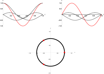
Figure 6: Top row: reproduction of the cosine (left) and sine (right) for $M=3$. The weighted and shifted basis functions are represented by dashed lines. The reconstructed parametric circle is shown in the bottom row (black) with the interpolatory control points (shown in red on the boundary of the circle).

Appendix F Reproduction of a Hyperbolic Paraboloid

A parameterization of a hyperbolic paraboloid is given by

$$\bm{\sigma}(u,v) =\begin{pmatrix}au\cosh(v)\\ bu\sinh(v)\\ hu^{2}\end{pmatrix},\quad(u,v)\in\mathbb{R}^{2},$$ (55)

where $a$, $b$, and $h$ are constants. The paraboloid (55) is polynomial in $u$ and hyperbolic in $v$. Hence, we choose $\bm{\alpha}_{1}=(0,0,0)$ and $\bm{\alpha}_{2}=\left(0,\frac{1}{M_{2}},\frac{-1}{M_{2}}\right)$ when expressing (55) as the tensor-product surface

$$\bm{\sigma}(u,v)=\sum_{k\in\mathbb{Z}}\sum_{l\in\mathbb{Z}}\bm{\sigma}[k,l]\phi_{\bm{\alpha}_{1}}(M_{1}u-k)\phi_{\bm{\alpha}_{2}}(M_{2}v-l).$$

To construct $\phi_{\bm{\alpha}_{1}}$, we have that $n_{0}=3$ and its support is equal to $N=2(n_{0}-1)=4$. The interpolator is expressed as

$$\phi_{\bm{\alpha}_{1}}(t)=\lambda[0]\beta_{\bm{\alpha}_{1}}(t)+\lambda[1]\bigg{(}\beta_{\bm{\alpha}_{1}}(t-\frac{1}{2})+\beta_{\bm{\alpha}_{1}}(t+\frac{1}{2})\bigg{)}.$$

Solving (25), we obtain $\lambda[0]=2$ and $\lambda[1]=-\frac{1}{2}$.

For the construction of $\phi_{\bm{\alpha}_{2}}$, we see that $n_{0}=3$, $N=2(n_{0}-1)=4$, and its support is also of size $4$. The interpolator is given by

$$\phi_{\bm{\alpha}_{2}}(t)=\lambda[0]\beta_{\bm{\alpha}_{2}}(t)+\lambda[1]\bigg{(}\beta_{\bm{\alpha}_{2}}(t-\frac{1}{2})+\beta_{\bm{\alpha}_{2}}(t+\frac{1}{2})\bigg{)}.$$

Solving (25) yields $\lambda[0]=1.968$ and $\lambda[1]=-0.489$. As in the previous example, the control points are obtained by sampling the surface, which leads to

$$\bm{\sigma}(u,v)\big{|}_{u=k,v=l}=\begin{pmatrix}a\frac{k}{M_{1}}\cosh(\frac{l}{M_{2}})\\ b\frac{k}{M_{1}}\sinh(\frac{l}{M_{2}})\\ h(\frac{k}{M_{1}})^{2}\end{pmatrix}.$$

We choose $(u,v)\in[-1,1]^{2}$, $M_{1}=M_{2}=3$, $a=b=4$ and $h=8$. The corresponding parameterization is

$$\bm{\sigma}(u,v)=\sum_{k=-M_{1}-1}^{M_{1}+1}\sum_{l=-M_{2}-1}^{M_{2}+1}\bm{\sigma}[k,l]\phi_{\bm{\alpha}_{1}}(M_{1}u-k)\phi_{\bm{\alpha}_{2}}(M_{2}v-l).$$

The hyperbolic paraboloid is illustrated in Figure 7.

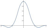
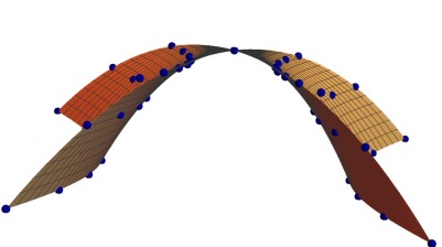
Figure 7: Hyperbolic paraboloid. On the left the interpolator $\phi_{\bm{\alpha}_{2}}$ is shown. ($\phi_{\bm{\alpha}_{1}}$ is shown in Figure 4.) On the right the reconstructed hyperbolic paraboloid with its interpolatory control points (blue dots) is shown.

References

References

- [1] C. Brechbühler, G. Gerig, O. Kübler, Parametrization of closed surfaces for 3-d shape description, Computer Vision and Image Understanding 61 (2) (1995) 154–170.
- [2] L. Romani, M. A. Sabin, The conversion matrix between uniform B-spline and Bezier representations, Comput. Aided Geom. Des. 21 (6) (2004) 549–560.
- [3] C. Conti, N. Dyn, C. Manni, M.-L. Mazure, Convergence of univariate non-stationary subdivision schemes via asymptotic similarity, Computer Aided Geometric Design 37 (2015) 1–8.
- [4] N. Dyn, D. Levin, J. A. Gregory, A 4-point interpolatory subdivision scheme for curve design, Computer Aided Geometric Design 4 (4) (1987) 257–268.
- [5] E. Cohen, T. Lyche, R. Riesenfeld, Discrete B-splines and subdivision techniques in computer-aided geometric design and computer graphics, Computer Graphics and Image Processing 14 (2) (1980) 87 – 111.
- [6] M. Botsch, L. Kobbelt, M. Pauly, P. Alliez, B. uno Levy, Polygon Mesh Processing, AK Peters, 2010.
- [7] R. Delgado-Gonzalo, N. Chenouard, M. Unser, Spline-based deforming ellipsoids for interactive 3D bioimage segmentation, IEEE Transactions on Image Processing 22 (10) (2013) 3926–3940.
- [8] J. Tang, S. Acton, Vessel boundary tracking for intravital microscopy via multiscale gradient vector flow snakes, IEEE Trans. Biomed. Eng. 51 (2) (2004) 316–324.
- [9] A. Dufour, R. Thibeaux, E. Labruyere, N. Guillen, J.-C. Olivo-Marin, 3-D Active meshes: Fast discrete deformable models for cell tracking in 3-D time-lapse microscopy, IEEE Transactions on Image Processing 20 (7) (2011) 1925–1937.
- [10] D. Barbosa, T. Dietenbeck, J. Schaerer, J. D’hooge, D. Friboulet, O. Bernard, B-Spline explicit active surfaces: An efficient framework for real-time 3-D region-based segmentation, IEEE Transactions on Image Processing 21 (1) (2012) 241–251.
- [11] D. Schmitter, R. Delgado-Gonzalo, G. Krueger, M. Unser, Atlas-free brain segmentation in 3D proton-density-like MRI images, in: Proceedings of the Eleventh IEEE International Symposium on Biomedical Imaging: From Nano to Macro (ISBI’14), Beijing, People’s Republic of China, 2014, pp. 629–632.
- [12] M. Audette, A. Chernikov, N. Chrisochoides, A review of mesh generation for medical simulators, Handbook of Real-World Applications in Modeling and Simulation 2 (2012) 261.
- [13] A. Garg, A. Sageman-Furnas, B. Deng, Y. Yue, E. Grinspun, M. Pauly, M. Wardetzky, Wire mesh design, ACM Trans. Graph. 33 (4) (2014) 66:1–66:12.
- [14] B. Deng, S. Bouaziz, M. Deuss, A. Kaspar, Y. Schwartzburg, M. Pauly, Interactive design exploration for constrained meshes, Computer-Aided Design 61 (2015) 13–23.
- [15] T. DeRose, M. Kass, T. Truong, Subdivision surfaces in character animation, in: Proceedings of the 25th Annual Conference on Computer Graphics and Interactive Techniques, SIGGRAPH ’98, ACM, New York, NY, USA, 1998, pp. 85–94.
- [16] N. Dyn, E. Farkhi, Spline subdivision schemes for compact sets. A survey, Serdica Mathematical Journal 28 (2002) 349–360.
- [17] N. Dyn, D. Levin, J. Yoon, Analysis of univariate nonstationary subdivision schemes with application to Gaussian-based interpolatory schemes, SIAM Journal on Mathematical Analysis 39 (2) (2007) 470–488.
- [18] C. Conti, L. Romani, Algebraic conditions on non-stationary subdivision symbols for exponential polynomial reproduction, Journal of Computational and Applied Mathematics 236 (4) (2011) 543 – 556.
- [19] M. Charina, C. Conti, L. Romani, Reproduction of exponential polynomials by multivariate non-stationary subdivision schemes with a general dilation matrix, Numerische Mathematik 127 (2) (2014) 223–254.
- [20] P. Novara, L. Romani, Building blocks for designing arbitrarily smooth subdivision schemes with conic precision, Journal of Computational and Applied Mathematics 279 (0) (2015) 67 – 79.
- [21] A. Badoual, D. Schmitter, V. Uhlmann, M. Unser, Multiresolution subdivision snakes, IEEE Transactions on Image Processing 26 (3) (2017) 1188–1201.
- [22] N. Dyn, L. David, A. Luzzatto, Exponentials reproducing subdivision schemes, Foundations of Computational Mathematics 3 (2) (2003) 187–206.
-
[23]
L. Piegl, On NURBS: A survey, IEEE
Comput. Graph. Appl. 11 (1) (1991) 55–71.
doi:10.1109/38.67702.
URL http://dx.doi.org/10.1109/38.67702 - [24] L. Piegl, W. Tiller, The NURBS Book, 2nd Edition, Springer Berlin Heidelberg, 2010.
- [25] D. F. Rogers, An Introduction to NURBS: With Historical Perspective, Morgan Kaufmann Publishers Inc., San Francisco, CA, USA, 2001.
- [26] D. Schmitter, C. Gaudet-Blavignac, D. Piccini, M. Unser, New parametric 3D snake for medical segmentation of structures with cylindrical topology, in: Proceedings of the 2015 IEEE International Conference on Image Processing (ICIP’15), Québec QC, Canada, 2015, pp. TEC–P21.1.
- [27] D. Schmitter, P. García-Amorena, M. Unser, Smoothly deformable spheres: Modeling, deformation, and interaction, in: Proceedings of the 2016 ACM Special Interest Group on Computer Graphics and Interactive Techniques Conference Asia: Technical Briefs (SIGGRAPH-TB’16), Macau, Macao Special Administrative Region of the People’s Republic of China, 2016, paper no. 2.
- [28] C. V. Beccari, G. Casciola, L. Romani, Construction and characterization of non-uniform local interpolating polynomial splines, J. Computational Applied Mathematics 240 (2013) 5–19.
- [29] M. Antonelli, C. Beccari, G. Casciola, A general framework for the construction of piecewise-polynomial local interpolants of minimum degree, Advances in Computational Mathematics 40 (4) (2014) 945–976.
- [30] M. Antonelli, C. V. Beccari, G. Casciola, High quality local interpolation by composite parametric surfaces, Computer Aided Geometric Design 46 (2016) 103 – 124.
- [31] E. Catmull, R. Rom, A class of local interpolating splines, Computer aided geometric design. Academic Press. (1974) 317–326.
- [32] R. Keys, Cubic convolution interpolation for digital image processing, IEEE Transactions on Acoustics, Speech and Signal Processing 29 (6) (1981) 1153–1160.
- [33] E. Meijering, M. Unser, A note on cubic convolution interpolation, IEEE Transactions on Image Processing 12 (4) (2003) 477–479.
- [34] D. Schmitter, R. Delgado-Gonzalo, M. Unser, Trigonometric interpolation kernel to construct deformable shapes for user-interactive applications, IEEE Signal Processing Letters 22 (11) (2015) 2097–2101.
- [35] D. Schmitter, R. Delgado-Gonzalo, M. Unser, A family of smooth and interpolatory basis functions for parametric curve and surface representation, Applied Mathematics and Computation 272 (1) (2016) 53–63.
- [36] A. Badoual, D. Schmitter, M. Unser, Locally refinable parametric snakes, in: Proceedings of the 2015 IEEE International Conference on Image Processing (ICIP’15), Québec QC, Canada, 2015, paper no. TEC-P21.2.
- [37] A. Badoual, D. Schmitter, M. Unser, Local refinement for 3d deformable parametric surfaces, in: Proceedings of the 2016 IEEE International Conference on Image Processing (ICIP’16), Phoenix AZ, USA, 2016, pp. 1086–1090.
- [38] M. Unser, T. Blu, Cardinal exponential splines: Part I—Theory and filtering algorithms, IEEE Transactions on Signal Processing 53 (4) (2005) 1425–1438.
- [39] M. Unser, Sampling—50 Years after Shannon, Proceedings of the IEEE 88 (4) (2000) 569–587.
- [40] J. Warren, H. Weimer, Subdivision Methods for Geometric Design: A Constructive Approach, 1st Edition, Morgan Kaufmann Publishers Inc., San Francisco, CA, USA, 2001.
- [41] C. Vonesch, T. Blu, M. Unser, Generalized Daubechies wavelet families, IEEE Transactions on Signal Processing 55 (9) (2007) 4415–4429.