Convergence Analysis of an Unconditionally Energy Stable Linear Crank-Nicolson Scheme for the Cahn-Hilliard Equation

Abstract

Efficient and unconditionally stable high order time marching schemes are very important but not easy to construct for nonlinear phase dynamics. In this paper, we propose and analysis an efficient stabilized linear Crank-Nicolson scheme for the Cahn-Hilliard equation with provable unconditional stability. In this scheme the nonlinear bulk force are treated explicitly with two second-order linear stabilization terms. The semi-discretized equation is a linear elliptic system with constant coefficients, thus robust and efficient solution procedures are guaranteed. Rigorous error analysis show that, when the time step-size is small enough, the scheme is second order accurate in time with a prefactor controlled by some lower degree polynomial of $1/\varepsilon$. Here $\varepsilon$ is the interface thickness parameter. Numerical results are presented to verify the accuracy and efficiency of the scheme.

1 Introduction

In this paper, we consider numerical approximation for the Cahn-Hilliard equation

$$\begin{cases}\phi_{t}=-\gamma\Delta(\varepsilon\Delta\phi-\dfrac{1}{\varepsilon}f(\phi)),&(x,t)\in\Omega\times(0,T],\\ \phi|_{t=0}=\phi_{0}(x),&x\in\Omega,\end{cases}$$ (1.1)

with Neumann boundary condition

$$\partial_{n}\phi=0,\;\partial_{n}(\varepsilon\Delta\phi-\dfrac{1}{\varepsilon}f(\phi))=0,\quad x\in\partial\Omega.$$ (1.2)

Here $\Omega\in R^{d},d=2,3$ is a bounded domain with a locally Lipschitz boundary, n is the outward normal, T is a given time, $\phi(x,t)$ is the phase-field variable. Function $f(\phi)=F^{\prime}(\phi)$, with $F(\phi)$ is a given energy potential with two local minima, e.g. the double well potential $F(\phi)=\frac{1}{4}(\phi^{2}-1)^{2}$. The two minima of $F$ produces two phases, with the typical thickness of the interface between two phases given by $\varepsilon$. $\gamma$ is a time relaxation parameter, its value is related to the time unit used in a physical process.

The equation (1.1) is a fourth-order partial differential equation, which is not easy to solve using a finite element method. However, if we introduce a new variable $\mu$, called chemical potential, for $-\varepsilon\Delta\phi+\dfrac{1}{\varepsilon}f(\phi)$, the equation (1.1) can be rewritten as a system of two second order equations

$$\begin{cases}\phi_{t}=\gamma\Delta\mu,&(x,t)\in\Omega\times(0,T],\\ \mu=-\varepsilon\Delta\phi+\dfrac{1}{\varepsilon}f(\phi),&(x,t)\in\Omega\times(0,T],\\ \phi|_{t=0}=\phi_{0}(x),&x\in\Omega.\end{cases}$$ (1.3)

The corresponding Neumann boundary condition reads

$$\partial_{n}\phi=0,\;\partial_{n}\mu=0,\quad x\in\partial\Omega.$$ (1.4)

The Cahn-Hilliard equation was originally introduced by Cahn-Hilliard [6] to describe the phase separation and coarsening phenomena in non-uniform systems such as alloys, glasses and polymer mixtures. If the term $\Delta\mu$ in equation (1.3) is replaced with $-\mu$, one get the Allen-Cahn equation, which was introduced by Allen and Cahn [2] to describe the motion of anti-phase boundaries in crystalline solids. The Cahn-Hilliard equation and the Allen-Cahn equation are two widely used phase-field model. In a phase-field model, the information of interface is encoded in a smooth phase function $\phi$. In most parts of the domain $\Omega$, the value of $\phi$ is close to local minima of $F$. The interface is a thin layer of thickness $\varepsilon$ connecting regions of different local minima. It is easy to deal with dynamical process involving morphology changes of interfaces using phase-field models. For this reason, phase field models have been the subject of many theoretical and numerical investigations (cf., for instance, [12], [15], [7], [8], [14], [17], [22], [33], [19], [30], [35], [9]).

However, numerically solving the phase-field equations is not an easy task, since the small parameter $\varepsilon$ in the Cahn-Hilliard equation makes the equation very stiff and requires a high spatial and temporal grid resolution. To design an energy stable scheme, one should respect the physical dissipation law of the Cahn-Hilliard system. In fact, the Cahn-Hilliard equation is $H^{-1}$ gradient flow of the Ginzburg-Laudau energy functional

$$E(\phi):=\int_{\Omega}\Big{(}\frac{\varepsilon}{2}|\nabla\phi|^{2}+\frac{1}{\varepsilon}F(\phi)\Big{)}dx$$ (1.5)

More precisely, by taking the inner product of (1.3) with $\mu$, and integration in time, we immediately find the following energy law for (1.3):

$$E(\phi(t))+\gamma\int_{0}^{t}\!\!\int_{\Omega}|\nabla\mu|^{2}dx=E(\phi_{0}),\;\forall\,t>0.$$ (1.6)

Since the nonlinear energy $F$ is neither a convex nor a concave function, treating it fully explicit or implicit in a time discretization will not lead to an efficient scheme. In fact, if the nonlinear force $f$ is treated fully explicitly, the resulting scheme will require a very tiny step-size to be stable(cf. for instance [35]). On the other hand, treating it fully implicitly will lead to a nonlinear system, for which the solution existence and uniqueness requires a restriction on step-size as well (cf. e.g. [19]). One popular approach to solve this dilemma is the convex splitting method [16, 17], in which the convex part of $F$ is treated implicitly and the concave part treated explicitly. The scheme is of first order accurate and unconditional stable. In each time step, one need solve a nonlinear system. The solution existence and uniqueness is guaranteed since the nonlinear system corresponds to a convex optimization problem. The convex splitting method was used widely, and several second order extensions were derived in different situations [9, 5, 11, 26], etc. Another type unconditional stable scheme is the secant-line method proposed by [12]. It is also used and extended in several other works, e.g. [22, 29, 18, 9, 25, 5, 45, 4]. Like the fully implicit method, the usual second order convex splitting method and the secant-type method for Cahn-Hilliard equation need a small time step-size to guarantee the semi-discretized nonlinear system has a unique solution (cf. for instance [12, 3]). To remove the restriction on time step-size, a diffusive three-step Crank-Nicolson scheme was introduced by [26] and [13] coupled with a second order convex splitting. After time-discretization, one get a nonlinear but unique solvable problem at each time step.

Recently, a new approach termed as invariant energy quadratization (IEQ) was introduced to handle the nonlinear energy. When applying to Cahn-Hilliard equation, it first appeared in [23, 24] as a Lagrange multiplier method. It then generalized by Yang et al. and successfully extended to handle several very complicated nonlinear phase-field models [40, 27, 43, 41, 42]. In the IEQ approach, a new variable which equals to the square root of $F$ is introduced, so the energy is written into a quadratic form in terms of the new variable. By using semi-implicit treatments to the nonlinear equation using new variables, one get a linear and energy stable scheme. It is straightforward to prove the unconditional stability for both first order and second order IEQ schemes. Comparing to the convex splitting approach, IEQ leads to well-structured linear system which is easier to solve. The modified energy in IEQ is an order-consistent approximation to the original system energy. At each time step, it needs to solve a linear system with time-varying coefficients.

Another trend of improving numerical schemes for phase-field models focuses on algorithm efficiency. Chen and Shen, and their coworkers [10, 44] studied stabilized some semi-implicit Fourier-spectral methods to the Cahn-Hilliard equation. The space variables are discretized by using a Fourier-spectral method whose convergence rate is exponential in contrast to the second order convergence of a usual finite-difference method, the time variable is discretized by using semi-implicit schemes which allow much larger time step sizes than explicit schemes. Xu and Tang in [39] introduced a different stabilized term to build stable large time-stepping semi-implicit methods for an epitaxial growth model. He et al [28] proposed similar large time-stepping methods for the Cahn-Hilliard equation, in which a stabilized term $A(\phi^{n+1}-\phi^{n})$ (resp. $A(\phi^{n+1}-2\phi^{n}+\phi^{n-1})$) is added to the nonlinear bulk force for the first order (resp. second order) scheme. Shen and Yang systematically studied stabilization schemes to the Allen-Cahn equation and the Cahn-Hilliard equation in mixed formulation [35]. They got first-order unconditionally energy stable schemes and second-order semi-implicit schemes with reasonable stability conditions. This idea was followed up in [21] for the stabilized Crank-Nicolson schemes for phase field models. In [37] another second-order time-accurate schemes for diffuse-interface models, which are of Crank-Nicolson type with a new convex-concave splitting of the energy and tumor-growth system. In above mentioned schemes, when the nonlinear force is treated explicitly, one can get energy stability with reasonable stabilization constant by introducing a proper stabilized term and a suitably truncated nonlinear $\tilde{f}(\phi)$ instead of $f(\phi)$ such that a uniform Lipschitz condition is satisfied. It is worth to mention that with no truncation made to double-well potential $F(\phi)$, Li et al [32, 31] proved that the energy stable can be obtained as well, but a much larger stability constant need be used.

Recently, we proposed two second-order unconditionally stable linear schemes based on Crank-Nicolson method (SL-CN) and second-order backward differentiation formula (SL-BDF2) for the Cahn-Hilliard equation[38]. In both schemes, explicit extrapolation is used for the nonlinear force with two extra stabilization terms which consist to the order of the schemes added to guarantee energy dissipation. The proposed methods have several merits: 1) They are second order accurate; 2) They lead to linear systems with constant coefficients after time discretization, thus robust and efficient solution procedures are guaranteed; 3) The stability analysis bases on Galerkin formulation, so both finite element methods and spectral methods can be used for spatial discretization to conserve volume fraction and satisfy discretized energy dissipation law. An optimal error estimate in $l^{\infty}(0,T;H^{-1})\cap l^{2}(0,T;H^{1})$ norm is obtained for the SL-BDF2 scheme in last paper. This paper aims to give an optimal error estimate of the SL-CN scheme.

The remain part of the paper is organized as follows. In Section 2, we present the stabilized linear semi-implicit Crank-Nicolson scheme for the Cahn-Hilliard equation and its unconditionally energy stability property. In Section 3, we carry out the error estimate to derive a convergence result that does not depend on $1/\varepsilon$ exponentially. A few numerical tests for a 2-dimensional square domain are included in Section 4 to verify our theoretical results. We end the paper with some concluding remarks in Section 5.

2 The stabilized linear semi-implicit Crank-Nicolson scheme

We first introduce some notations which will be used throughout the paper. We use $\|\cdot\|_{m,p}$ to denote the standard norm of the Sobolev space $W^{m,p}(\Omega)$. In particular, we use $\|\cdot\|_{L^{p}}$ to denote the norm of $W^{0,p}(\Omega)=L^{p}(\Omega)$; $\|\cdot\|_{{m}}$ to denote the norm of $W^{m,2}(\Omega)=H^{m}(\Omega)$; and $\|\cdot\|$ to denote the norm of $W^{0,2}(\Omega)=L^{2}(\Omega)$. Let $(\cdot,\cdot)$ represent the $L^{2}$ inner product. In addition, define for $p\geq 0$

$$H^{-p}(\Omega):=\left(H^{p}(\Omega)\right)^{*},\quad H_{0}^{-p}(\Omega):=\left\{u\in H^{-p}(\Omega)\mid\,\langle u,1\rangle_{p}=0\right\},$$

where $\langle\cdot,\cdot\rangle_{p}$ stands for the dual product between $H^{p}(\Omega)$ and $H^{-p}(\Omega)$. We denote $L_{0}^{2}(\Omega):=H_{0}^{0}(\Omega)$. For $v\in L_{0}^{2}(\Omega)$, let $-\Delta^{-1}v:=v_{1}\in H^{1}(\Omega)\cap L_{0}^{2}(\Omega)$, where $v_{1}$ is the solution to

$$-\Delta v_{1}=v\ \ {\rm in}\ \Omega,\quad\ \frac{\partial v_{1}}{\partial n}=0\ \ {\rm on}\ \partial\Omega,$$

and $\|v\|_{-1}:=\sqrt{(v,-\Delta^{-1}v)}$.

For any given function $\phi(t)$ of $t$, we use $\phi^{n}$ to denote an approximation of $\phi(n\tau)$, where $\tau$ is the step-size. We will frequently use the shorthand notations: $\delta_{t}\phi^{n+1}:=\phi^{n+1}-\phi^{n}$, $\delta_{tt}\phi^{n+1}:=\phi^{n+1}-2\phi^{n}+\phi^{n-1}$, and $\hat{\phi}^{n+\frac{1}{2}}:=\frac{3}{2}\phi^{n}-\frac{1}{2}\phi^{n-1}$. Following identities and inequality will be used frequently.

$$2(h^{n+1}-h^{n},h^{n+1})=\|h^{n+1}\|^{2}-\|h^{n}\|^{2}+\|h^{n+1}-h^{n}\|^{2},$$ (2.7)

$$(u,v)\leq\|u\|_{-1}\|\nabla v\|,\quad\forall\ u\in L_{0}^{2},v\in H^{1}.$$ (2.8)

Suppose $\phi^{0}=\phi_{0}(\cdot)$ and $\phi^{1}\approx\phi(\cdot,\tau)$ are given, our stabilized liner Crank-Nicolson scheme (abbr. SL-CN) calculates $\phi^{n+1},n=1,2,\ldots,N=T/\tau-1$ iteratively, using

$$\frac{\phi^{n+1}-\phi^{n}}{\tau}=\gamma\Delta\mu^{n+\frac{1}{2}},$$ (2.9)

$$\mu^{n+\frac{1}{2}}=-\varepsilon\Delta\Big{(}\frac{\phi^{n+1}+\phi^{n}}{2}\Big{)}+\frac{1}{\varepsilon}f\Big{(}\frac{3}{2}\phi^{n}-\frac{1}{2}\phi^{n-1}\Big{)}-A\tau\Delta\delta_{t}\phi^{n+1}+B\delta_{tt}\phi^{n+1},$$ (2.10)

where $A$ and $B$ are two non-negative constants to stabilize the scheme.

To prove energy stability of the numerical schemes, we assume that the derivative of $f$ in equation (1.3) is uniformly bounded, i.e.

$$\max_{\phi\in\mathbf{R}}|f^{\prime}(\phi)|\leq L,$$ (2.11)

where $L$ is a non-negative constant. Note that, although most of the nonlinear potential, e.g. the double-well poential doesn’t satisfy (2.11), the above assumption is reasonable since: 1) physically $\phi$ should take values in $[-1,1]$; 2) it was proved by Caffarelli and Muler [8] that an $L^{\infty}$ bound exists for Cahn-Hilliard equation with a potential having linear growth for $|\phi|>1$, 3) it is proved by [1] and [20] that when a proper initial condition is given, the Cahn-Hilliard equation converges to Hele-Shaw problem when $\varepsilon\rightarrow 0$. If the corresponding Hele-Shaw problem has a global (in time) classical solution, then the solution to the Cahn-Hilliard equation has a $L^{\infty}$ bound.

Theorem 2.1.

Under the condition

$$A\geq\dfrac{L^{2}}{16\varepsilon^{2}}\gamma,\quad B\geq\dfrac{L}{2\varepsilon},$$ (2.12)

the following energy dissipation law

$$E_{CN}^{n+1}\leq E_{CN}^{n}-\Big{(}2\sqrt{\frac{A}{\gamma}}-\frac{L}{2\varepsilon}\Big{)}\|\delta_{t}\phi^{n+1}\|^{2}-\Big{(}\frac{B}{2}-\frac{L}{4\varepsilon}\Big{)}\|\delta_{tt}\phi^{n+1}\|^{2},\hskip 28.45274pt\forall n\geq 1,$$ (2.13)

holds for the scheme (2.9)-(2.10), where

$$E_{CN}^{n+1}=E(\phi^{n+1})+\Big{(}\frac{L}{4\varepsilon}+\frac{B}{2}\Big{)}\|\delta_{t}\phi^{n+1}\|^{2}.$$ (2.14)

Proof.

Pairing (2.9) with $\tau\mu^{n+\frac{1}{2}}$, (2.10) with $-\delta_{t}\phi^{n+1}$, and combining the results, we get

$$\begin{split}&\frac{\varepsilon}{2}(\|\nabla\phi^{n+1}\|^{2}-\|\nabla\phi^{n}\|^{2})+\frac{1}{\varepsilon}(f\big{(}\hat{\phi}^{n+\frac{1}{2}}\big{)},\delta_{t}\phi^{n+1})\\ =&-\gamma\tau\|\nabla\mu^{n+\frac{1}{2}}\|^{2}-A\tau\|\nabla\delta_{t}\phi^{n+1}\|^{2}-B(\delta_{tt}\phi^{n+1},\delta_{t}\phi^{n+1}).\end{split}$$ (2.15)

Pairing (2.9) with $2\sqrt{\frac{A}{\gamma}}\tau\delta_{t}\phi^{n+1}$, then using Cauchy-Schwartz inequality, we get

$$2\sqrt{\tfrac{A}{\gamma}}\|\delta_{t}\phi^{n+1}\|^{2}=-2\sqrt{A\gamma}\tau(\nabla\mu^{n+\frac{1}{2}},\nabla\delta_{t}\phi^{n+1})\leq\gamma\tau\|\nabla\mu^{n+\frac{1}{2}}\|^{2}+A\tau\|\nabla\delta_{t}\phi^{n+1}\|^{2}.$$ (2.16)

To handle the term involving $f$, we expand $F(\phi^{n+1})$ and $F(\phi^{n})$ at $\hat{\phi}^{n+\frac{1}{2}}$ as

$$F(\phi^{n+1}) =F(\hat{\phi}^{n+\frac{1}{2}})+f(\hat{\phi}^{n+\frac{1}{2}})(\phi^{n+1}-\hat{\phi}^{n+\frac{1}{2}})+\frac{1}{2}f^{\prime}(\xi^{n}_{1})(\phi^{n+1}-\hat{\phi}^{n+\frac{1}{2}})^{2},$$

$$F(\phi^{n}) =F(\hat{\phi}^{n+\frac{1}{2}})+f(\hat{\phi}^{n+\frac{1}{2}})(\phi^{n}-\hat{\phi}^{n+\frac{1}{2}})+\frac{1}{2}f^{\prime}(\xi^{n}_{2})(\phi^{n}-\hat{\phi}^{n+\frac{1}{2}})^{2},$$

where $\xi^{n}_{1}$ is a number between $\phi^{n+1}$ and $\hat{\phi}^{n+\frac{1}{2}}$, $\xi^{n}_{2}$ is a number between $\phi^{n}$ and $\hat{\phi}^{n+\frac{1}{2}}$. Taking the difference of above two equations, we have

$$\begin{split}&F(\phi^{n+1})-F(\phi^{n})-f(\hat{\phi}^{n+\frac{1}{2}})(\phi^{n+1}-\phi^{n})\\ ={}&\frac{1}{2}f^{\prime}(\xi^{n}_{1})\left[(\phi^{n+1}-\hat{\phi}^{n+\frac{1}{2}})^{2}-(\phi^{n}-\hat{\phi}^{n+\frac{1}{2}})^{2}\right]-\frac{1}{2}(f^{\prime}(\xi^{n}_{2})-f^{\prime}(\xi^{n}_{1}))(\phi^{n}-\hat{\phi}^{n+\frac{1}{2}})^{2}\\ ={}&\frac{1}{2}f^{\prime}(\xi^{n}_{1})\delta_{t}\phi^{n+1}\delta_{tt}\phi^{n+1}-\frac{1}{8}(f^{\prime}(\xi^{n}_{2})-f^{\prime}(\xi^{n}_{1}))(\delta_{t}\phi^{n})^{2}\\ \leq{}&\frac{L}{4}(|\delta_{t}\phi^{n+1}|^{2}+|\delta_{tt}\phi^{n+1}|^{2})+\frac{L}{4}|\delta_{t}\phi^{n}|^{2}.\end{split}$$

Multiplying the above equation with $\dfrac{1}{\varepsilon}$, then taking integration leads to

$$\frac{1}{\varepsilon}(F(\phi^{n+1})-F(\phi^{n})-f(\hat{\phi}^{n+\frac{1}{2}})\delta_{t}\phi^{n+1},1)\leq\frac{L}{4\varepsilon}(\|\delta_{t}\phi^{n+1}\|^{2}+\|\delta_{tt}\phi^{n+1}\|^{2}+\|\delta_{t}\phi^{n}\|^{2}).$$ (2.17)

For the term involving $B$, by using identity (2.7) with $h^{n+1}=\delta_{t}\phi^{n+1}$, one get

$$-B(\delta_{tt}\phi^{n+1},\delta_{t}\phi^{n+1})=-\frac{B}{2}\|\delta_{t}\phi^{n+1}\|^{2}+\frac{B}{2}\|\delta_{t}\phi^{n}\|^{2}-\frac{B}{2}\|\delta_{tt}\phi^{n+1}\|^{2}.$$ (2.18)

Summing up (2.15)-(2.18), we obtain

$$\begin{split}&\frac{\varepsilon}{2}(\|\nabla\phi^{n+1}\|^{2}-\|\nabla\phi^{n}\|^{2})+\frac{1}{\varepsilon}(F(\phi^{n+1})-F(\phi^{n}),1)+\frac{B}{2}\|\delta_{t}\phi^{n+1}\|^{2}-\frac{B}{2}\|\delta_{t}\phi^{n}\|^{2}\\ \leq&-2\sqrt{\frac{A}{\gamma}}\|\delta_{t}\phi^{n+1}\|^{2}+\frac{L}{4\varepsilon}\|\delta_{t}\phi^{n+1}\|^{2}+\frac{L}{4\varepsilon}\|\delta_{t}\phi^{n}\|^{2}-\frac{B}{2}\|\delta_{tt}\phi^{n+1}\|^{2}+\frac{L}{4\varepsilon}\|\delta_{tt}\phi^{n+1}\|^{2},\end{split}$$ (2.19)

which is the energy estimate (2.13). ∎

Remark 2.1.

Note that, if $B=0$, we can take $A\geq\dfrac{L^{2}\gamma}{4\varepsilon^{2}}$ to make the SL-CN scheme (2.9)-(2.10) unconditionally stable as well. However, when $A=0$, we can’t prove an unconditional stability for $B\sim O(\varepsilon^{-1})$ or $B\sim O(\varepsilon^{-2})$.

Remark 2.2.

The constant $A$ defined in equation (2.12) seems to be quite large when $\varepsilon$ is small, but it is not necessarily true. Since usually $\gamma$ is a small constant related to $\varepsilon$. For example, it was pointed out in [34] that, the Cahn-Hilliard equation coupled with the Navier-Stokes equations have a sharp-interface limit when $O(\varepsilon^{3})\leq\gamma\leq O(\varepsilon)$, while $\gamma\sim O(\varepsilon^{2})$ gives the fastest convergence. On the other hand, the numerical results in Section 4 shows that in practice $A$ can take much smaller values than those defined in (2.12) when nonzero $B$ values are used.

Remark 2.3.

The discrete Energy $E_{C}$ defined in equation (2.14) is a first order approximation to the original energy $E$, since $\|\delta_{t}\phi^{n+1}\|^{2}\sim O(\tau^{2})$. On the other side, summing up the equation (2.13) for $n=1,\ldots,N$, we get

$$E^{N+1}_{CN}+\sum_{n=1}^{N}\left(\Big{(}2\sqrt{\frac{A}{\gamma}}-\frac{L}{2\varepsilon}\Big{)}\|\delta_{t}\phi^{n+1}\|^{2}-\Big{(}\frac{B}{2}-\frac{L}{4\varepsilon}\Big{)}\|\delta_{tt}\phi^{n+1}\|^{2}\right)\leq E^{1}_{CN}.$$ (2.20)

By taking $N\rightarrow\infty$, we get $\delta_{t}\phi^{n+1}\rightarrow 0$, which means the system will eventually converge to a steady state. By equation (2.9) and (2.10), this steady state is a critical point of the original energy functional $E$.

3 Convergence analysis

In this section, we shall establish error estimate of the SL-CN scheme. We will shown that, if the interface is well developed in the initial condition, the error bounds depend on $\frac{1}{\varepsilon}$ only in some lower polynomial order for small $\varepsilon$. Let $\phi(t^{n})$ be the exact solution at time $t=t^{n}$ to equation of (1.3) and $\phi^{n}$ be the solution to the time discrete numerical scheme (2.9)-(2.10), we define error function $e^{n}:=\phi^{n}-\phi(t^{n})$. Obviously $e^{0}=0$.

Before presenting the detailed error analysis, we first make some assumptions. For simplicity, we take $\gamma=1$ in this section, and assume $0<\varepsilon<1$. We use notation $\lesssim$ in the way that $f\lesssim g$ means that $f\leq Cg$ with positive constant $C$ independent of $\tau$ and $\varepsilon$.

Assumption 3.1.

We make following assumptions on $f$:

1. $F\in C^{4}(\mathbf{R})$, $F(\pm 1)=0$, and $F>0$ elsewhere. There exist two non-negative constants $B_{0},B_{1}$, such that

   $$\phi^{2}\leq B_{0}+B_{1}F(\phi),\quad\forall\;\phi\in\mathbf{R}.$$ (3.21)

2. $f=F^{\prime}$. $f^{\prime}$ and $f^{\prime\prime}$ are uniformly bounded, or, $f$ satisfies (2.11) and

   $$\max_{\phi\in\mathbf{R}}|f^{\prime\prime}(\phi)|\leq L_{2},$$ (3.22)

   where $L_{2}$ is a non-negative constant.

Assumption 3.2.

We assume that there exist positive constants $m_{0}$ and non-negative constants $\sigma_{1},\sigma_{2},\sigma_{3}$ such that

$$m_{0}:=\frac{1}{|\Omega|}\int_{\Omega}\phi^{0}(x){\rm d}x\in(-1,1),$$ (3.23)

$$E(\phi^{0}):=\frac{\varepsilon}{2}\|\nabla\phi^{0}\|^{2}+\frac{1}{\varepsilon}\|F(\phi^{0})\|_{L^{1}}\lesssim\varepsilon^{-2\sigma_{1}}.$$ (3.24)

$$\|\mu^{0}\|_{H^{l}}:=\|-\varepsilon\Delta\phi^{0}+\frac{1}{\varepsilon}f(\phi^{0})\|_{H^{l}}\lesssim\varepsilon^{-2\sigma_{2+l}},\ l=0,1.$$ (3.25)

We also assume that an appropriate scheme is used to calculate the numerical solution at first step, such that

$$m_{1}:=\frac{1}{|\Omega|}\int_{\Omega}\phi^{1}(x){\rm d}x=m_{0},\qquad E_{\varepsilon}(\phi^{1})\leq E_{\varepsilon}(\phi^{0})\lesssim\varepsilon^{-2\sigma_{1}},$$ (3.26)

$$\|\delta_{t}\phi^{1}\|^{2}\lesssim\varepsilon^{-2\sigma_{1}},$$ (3.27)

then

$$E_{CN}^{1}\lesssim\varepsilon^{-2\sigma_{1}}+\varepsilon^{-2\sigma_{1}-1},$$ (3.28)

and exist a constant $\sigma_{0}>0$,

$$\|e^{1}\|_{-1}^{2}+\|e^{1}\|^{2}+\varepsilon\|\nabla e^{1}\|^{2}\lesssim\varepsilon^{-\sigma_{0}}\tau^{4}.$$ (3.29)

Lemma 3.1.

Suppose that $f$ satisfies Assumption 3.1, $\phi_{0}\in H^{2}(\Omega)$. Then, the following estimates holds for the numerical solution of (2.9)-(2.10)

$$\frac{1}{|\Omega|}\int_{\Omega}\phi^{n}(x){\rm d}x=m_{0},\quad n=1,\ldots,N+1,$$ (3.30)

$$E_{CN}^{n+1}\leq E_{CN}^{1}\lesssim\varepsilon^{-2\sigma_{1}-1}.$$ (3.31)

Proof.

(i) Equation (3.30) is obtained by integrating equation (2.9).

(ii) Equation (3.31) is a direct result of the energy estimate (2.13) and (3.28). ∎

Some regularities of exact solution $\phi(t)$ are necessary for the error estimates.

Assumption 3.3.

Suppose the exact solution of (1.3) have the following regularities:

1. $\Delta^{-1}\phi(t)\in W^{2,2}(0,\infty;H^{-1})$, or

   $$\int_{0}^{\infty}\|\partial_{tt}\Delta^{-1}\phi(t)\|_{-1}^{2}{\rm d}t\leq\varepsilon^{-\rho_{1}},$$

2. $\phi(t)\in W^{2,2}(0,\infty;H^{-1}\bigcap H^{3})$, or

   $$\int_{0}^{\infty}\|\partial_{tt}\phi(t)\|_{-1}^{2}{\rm d}t \leq\varepsilon^{-\rho_{2}},\quad \int_{0}^{\infty}\|\partial_{tt}\phi(t)\|^{2}{\rm d}t \leq\varepsilon^{-\rho_{3}},$$

   $$\int_{0}^{\infty}\|\partial_{tt}\nabla\phi(t)\|^{2}{\rm d}t \leq\varepsilon^{-\rho_{4}},\quad \int_{0}^{\infty}\|\partial_{tt}\nabla\Delta\phi(t)\|^{2}{\rm d}t \leq\varepsilon^{-\rho_{5}},$$

3. $\phi(t)\in W^{1,2}(0,\infty;H^{3})$, or

   $$\int_{0}^{\infty}\|\partial_{t}\nabla\phi(t)\|^{2}{\rm d}t\leq\varepsilon^{-\rho_{6}},\quad\int_{0}^{\infty}\|\partial_{t}\nabla\Delta\phi(t)\|^{2}{\rm d}t\leq\varepsilon^{-\rho_{7}},\quad\int_{0}^{\infty}\|\partial_{t}\phi(t)\|^{2}{\rm d}t\leq\varepsilon^{-\rho_{8}}.$$

Here $\rho_{j},j=1,2,3,4,5,6,7,8$ are non-negative constants which depend on $\sigma_{1},\sigma_{2},\sigma_{3}.$

We first carry out a coarse error estimate using a standard approach for time semi-discretized schemes.

Proposition 3.1.

(Coarse error estimate) Suppose that $A,B$ are any non-negative number. Then for all $N\geq 1$, we have estimate

$$\begin{split}&\|e^{N+1}\|_{-1}^{2}+\frac{\varepsilon\tau}{4}\|\nabla\frac{e^{N+1}+e^{N}}{2}\|^{2}+A\tau^{2}\|\nabla e^{N+1}\|^{2}+B\tau\|e^{N+1}\|^{2}\\ \lesssim&\varepsilon^{-\max\{\rho_{1}+1,\rho_{2}+3,\rho_{4}-1,\rho_{6}+5\}}\tau^{4}+A\tau^{2}\|\nabla e^{N}\|^{2}+B\tau\|e^{N}\|^{2}\\ &+\Big{(}1+\frac{4B^{2}\tau}{\varepsilon}+\frac{9L^{2}\tau}{\varepsilon^{3}}\Big{)}\|e^{N}\|_{-1}^{2}+\Big{(}\frac{4B^{2}\tau}{\varepsilon}+\frac{L^{2}\tau}{\varepsilon^{3}}\Big{)}\|e^{N-1}\|^{2}_{-1},\quad\forall\ \tau>0.\\ \end{split}$$ (3.32)

and

$$\begin{split}&\max_{1\leq n\leq N}\Big{(}\|e^{n+1}\|_{-1}^{2}+A\tau^{2}\|\nabla e^{n+1}\|^{2}+B\tau\|e^{n+1}\|^{2}\Big{)}+\frac{\varepsilon\tau}{4}\sum_{n=1}^{N}\|\nabla\frac{e^{n+1}+e^{n}}{2}\|^{2}\\ \lesssim&\mathrm{exp}\Big{(}\frac{16B^{2}T}{\varepsilon}+\frac{20L^{2}T}{\varepsilon^{3}}\Big{)}\varepsilon^{-\max\{\rho_{1}+1,\rho_{2}+3,\rho_{4}-1,\rho_{6}+5,\sigma_{0}+3\}}\tau^{4},\quad\forall\ \tau<1.\end{split}$$ (3.33)

The index $\sigma_{0}+3$ in (3.33) can be replaced with $\sigma_{0}$ if we take $\tau<\varepsilon^{1.5}$.

Proof.

The following equations for the error function hold:

$$\frac{e^{n+1}-e^{n}}{\tau}=\Delta(\mu^{n+\frac{1}{2}}-\mu(t^{n+\frac{1}{2}}))+\Big{(}\phi^{n+\frac{1}{2}}_{t}-\frac{\phi(t^{n+1})-\phi(t^{n})}{\tau}\Big{)},$$ (3.34)

$$\begin{split}\mu^{n+\frac{1}{2}}-\mu(t^{n+\frac{1}{2}})=&-\varepsilon\Delta\Big{(}\frac{\phi^{n+1}+\phi^{n}}{2}-\phi(t^{n+\frac{1}{2}})\Big{)}+\frac{1}{\varepsilon}\Big{(}f(\frac{3}{2}\phi^{n}-\frac{1}{2}\phi^{n-1})-f(\phi(t^{n+\frac{1}{2}}))\Big{)}\\ &-A\tau\Delta\delta_{t}\phi^{n+1}+B\delta_{tt}\phi^{n+1}.\end{split}$$ (3.35)

Pairing (3.34) with $-\Delta^{-1}\big{(}\frac{e^{n+1}+e^{n}}{2}\big{)}$, adding (3.35) paired with $-\big{(}\frac{e^{n+1}+e^{n}}{2}\big{)}$, we get

$$\begin{split}&\frac{1}{2\tau}(\|e^{n+1}\|_{-1}^{2}-\|e^{n}\|_{-1}^{2})+\varepsilon\|\nabla\frac{e^{n+1}+e^{n}}{2}\|^{2}+\frac{A\tau}{2}(\|\nabla e^{n+1}\|^{2}-\|\nabla e^{n}\|^{2})\\ =&-\Big{(}R_{1}^{n+1},\Delta^{-1}\frac{e^{n+1}+e^{n}}{2}\Big{)}+A\Big{(}\Delta R_{2}^{n+1},\frac{e^{n+1}+e^{n}}{2}\Big{)}-B\Big{(}R_{3}^{n+1},\frac{e^{n+1}+e^{n}}{2}\Big{)}\\ &+\varepsilon\Big{(}\Delta R_{4}^{n+1},\frac{e^{n+1}+e^{n}}{2}\Big{)}-B\Big{(}\delta_{tt}e^{n+1},\frac{e^{n+1}+e^{n}}{2}\Big{)}\\ &-\frac{1}{\varepsilon}\Big{(}f(\frac{3}{2}\phi^{n}-\frac{1}{2}\phi^{n-1})-f(\phi(t^{n+\frac{1}{2}})),\frac{e^{n+1}+e^{n}}{2}\Big{)}\\ =&:J_{1}+J_{2}+J_{3}+J_{4}+J_{5}+J_{6}=:J,\\ \end{split}$$ (3.36)

where

$$R_{1}^{n+1}=\phi_{t}^{n+\frac{1}{2}}-\frac{\phi(t^{n+1})-\phi(t^{n}))}{\tau},$$ (3.37)

$$R_{2}^{n+1}=\tau(\phi(t^{n+1})-\phi(t^{n})),$$ (3.38)

$${R_{3}^{n+1}=}\phi(t^{n+1})-2\phi(t^{n})+\phi(t^{n-1}),$$ (3.39)

$${R_{4}^{n+1}=}\frac{\phi(t^{n+1})+\phi(t^{n})}{2}-\phi(t^{n+\frac{1}{2}}).$$ (3.40)

For the right hand of (3.36), by using Cauchy-Schwartz inequality, we obtain the following estimate:

$$J_{1}=-\Big{(}R_{1}^{n+1},\Delta^{-1}\frac{e^{n+1}+e^{n}}{2}\Big{)}\leq\frac{1}{\eta}\|\Delta^{-1}R_{1}^{n+1}\|_{-1}^{2}+\frac{\eta}{4}\|\nabla\frac{e^{n+1}+e^{n}}{2}\|^{2},$$ (3.41)

$$J_{2}=A\Big{(}\Delta R_{2}^{n+1},\frac{e^{n+1}+e^{n}}{2}\Big{)}\leq\frac{A^{2}}{\eta}\|\nabla R_{2}^{n+1}\|^{2}+\frac{\eta}{4}\|\nabla\frac{e^{n+1}+e^{n}}{2}\|^{2},$$ (3.42)

$$J_{3}=-B\Big{(}R_{3}^{n+1},\frac{e^{n+1}+e^{n}}{2}\Big{)}\leq\frac{B^{2}}{\eta}\|R_{3}^{n+1}\|_{-1}^{2}+\frac{\eta}{4}\|\nabla\frac{e^{n+1}+e^{n}}{2}\|^{2},$$ (3.43)

$$J_{4}=\varepsilon\Big{(}\Delta R_{4}^{n+1},\frac{e^{n+1}+e^{n}}{2}\Big{)}\leq\frac{\varepsilon^{2}}{\eta}\|\nabla R_{4}^{n+1}\|^{2}+\frac{\eta}{4}\|\nabla\frac{e^{n+1}+e^{n}}{2}\|^{2}.$$ (3.44)

For $J_{5}$ of the right side of (3.36), by using $\delta_{tt}e^{n+1}=\delta_{t}e^{n+1}-\delta_{t}e^{n}$, we have

$$\begin{split}J_{5}&=-B\Big{(}\delta_{tt}e^{n+1},\frac{e^{n+1}+e^{n}}{2}\Big{)}\\ &=-\frac{B}{2}(\|e^{n+1}\|^{2}-\|e^{n}\|^{2})+\frac{B}{2}(\delta_{t}e^{n},e^{n+1}+e^{n})\\ &\leq-\frac{B}{2}(\|e^{n+1}\|^{2}-\|e^{n}\|^{2})+\frac{B^{2}}{\eta}\|e^{n}-e^{n-1}\|^{2}_{-1}+\frac{\eta}{4}\|\nabla\frac{e^{n+1}+e^{n}}{2}\|^{2}.\end{split}$$ (3.45)

$$\begin{split}J_{6}&=-\frac{1}{\varepsilon}\Big{(}f(\frac{3}{2}\phi^{n}-\frac{1}{2}\phi^{n-1})-f(\phi(t^{n+\frac{1}{2}})),\frac{e^{n+1}+e^{n}}{2}\Big{)}\\ &\leq\frac{L}{\varepsilon}\Big{(}|R_{5}^{n+1}|,|\frac{e^{n+1}+e^{n}}{2}|\Big{)}+\frac{L}{\varepsilon}\Big{(}|\frac{3}{2}e^{n}-\frac{1}{2}e^{n-1}|,|\frac{e^{n+1}+e^{n}}{2}|\Big{)}\\ &\leq\frac{L^{2}}{\varepsilon^{2}\eta}\Big{(}\|R_{5}^{n+1}\|_{-1}^{2}+\|\frac{3}{2}e^{n}-\frac{1}{2}e^{n-1}\|_{-1}^{2}\Big{)}+\frac{\eta}{2}\|\nabla\frac{e^{n+1}+e^{n}}{2}\|^{2},\end{split}$$ (3.46)

where

$${R_{5}^{n+1}=}\frac{3}{2}\phi(t^{n})-\frac{1}{2}\phi(t^{n-1})-\phi(t^{n+\frac{1}{2}}).$$ (3.47)

For the $R_{1},\ldots,R_{5}$ terms, we have following estimates:

$$\|\Delta^{-1}R_{1}^{n+1}\|_{-1}^{2}\lesssim\tau^{3}\int_{t^{n}}^{t^{n+1}}\|\partial_{tt}\Delta^{-1}\phi(t)\|_{-1}^{2}{\rm d}t,$$ (3.48)

$$\|\nabla R_{2}^{n+1}\|^{2}\lesssim\tau^{3}\int_{t^{n}}^{t^{n+1}}\|\partial_{t}\nabla\phi(t)\|^{2}{\rm d}t,$$ (3.49)

$$\|R_{3}^{n+1}\|_{-1}^{2}\lesssim 6\tau^{3}\int_{t^{n-1}}^{t^{n+1}}\|\partial_{tt}\phi(t)\|_{-1}^{2}{\rm d}t,$$ (3.50)

$$\|\nabla R_{4}^{n+1}\|^{2}\lesssim\tau^{3}\int_{t^{n}}^{t^{n+1}}\|\partial_{tt}\nabla\phi(t)\|^{2}{\rm d}t,$$ (3.51)

$$\|R_{5}^{n+1}\|_{-1}^{2}\lesssim\tau^{3}\int_{t^{n-1}}^{t^{n+1}}\|\partial_{tt}\phi(t)\|_{-1}^{2}{\rm d}t.$$ (3.52)

Substituting $J_{1},\cdots,J_{6}$ into (3.36), we have

$$\begin{split}&\frac{1}{2\tau}(\|e^{n+1}\|_{-1}^{2}-\|e^{n}\|_{-1}^{2})+\varepsilon\|\nabla\frac{e^{n+1}+e^{n}}{2}\|^{2}+\frac{A\tau}{2}(\|\nabla e^{n+1}\|^{2}-\|\nabla e^{n}\|^{2})\\ &+\frac{B}{2}(\|e^{n+1}\|^{2}-\|e^{n}\|^{2})\\ \lesssim&\frac{1}{\eta}C_{1}^{n+1}\tau^{3}+\frac{7\eta}{4}\|\nabla\frac{e^{n+1}+e^{n}}{2}\|^{2}+\frac{B^{2}}{\eta}\|e^{n}-e^{n-1}\|^{2}_{-1}+\frac{L^{2}}{\varepsilon^{2}\eta}\|\frac{3}{2}e^{n}-\frac{1}{2}e^{n-1}\|_{-1}^{2},\end{split}$$ (3.53)

where

$$\begin{split}C_{1}^{n+1}=&\int_{t_{n}}^{t_{n+1}}(\|\partial_{tt}\Delta^{-1}\phi(t)\|_{-1}^{2}+A^{2}\|\partial_{t}\nabla\phi(t)\|^{2}){\rm d}t\\ &+\int_{t_{n-1}}^{t_{n+1}}\Big{(}\Big{(}B^{2}+\frac{L^{2}}{\varepsilon^{2}}\Big{)}\|\partial_{tt}\phi(t)\|_{-1}^{2}+\varepsilon^{2}\|\partial_{tt}\nabla\phi(t)\|^{2}\Big{)}{\rm d}t.\end{split}$$

Taking $\eta=\varepsilon/2$, multiplying (3.53) by $2\tau$, we obtain (3.32) by using inequality $\|a+b\|^{2}\leq 2\|a\|^{2}+2\|b\|^{2}$ and estimates (3.48)-(3.52). Then by summing (3.53) for $n=1\cdots N$, we obtain

$$\begin{split}&(\|e^{N+1}\|_{-1}^{2}-\|e^{1}\|_{-1}^{2})+\frac{\varepsilon\tau}{4}\sum_{n=1}^{N}\|\nabla\frac{e^{n+1}+e^{n}}{2}\|^{2}+A\tau^{2}(\|\nabla e^{N+1}\|^{2}-\|\nabla e^{1}\|^{2})\\ &+B\tau(\|e^{N+1}\|^{2}-\|e^{1}\|^{2})\\ \lesssim&\frac{4}{\varepsilon}C_{1}\tau^{4}+\Big{(}\frac{16B^{2}\tau}{\varepsilon}+\frac{20L^{2}\tau}{\varepsilon^{3}}\Big{)}\sum_{n=1}^{N}\|e^{n}\|_{-1}^{2},\\ \end{split}$$ (3.54)

where

$$\begin{split}C_{1}=&\sum_{n=1}^{N}C_{1}^{n+1}\\ \leq&\int_{0}^{T}\Big{(}\|\partial_{tt}\Delta^{-1}\phi(t)\|_{-1}^{2}+A^{2}\|\partial_{t}\nabla\phi(t)\|^{2}+2\Big{(}B^{2}+\frac{L^{2}}{\varepsilon^{2}}\Big{)}\|\partial_{tt}\phi(t)\|_{-1}^{2}\\ &+2\varepsilon^{2}\|\partial_{tt}\nabla\phi(t)\|^{2}\Big{)}{\rm d}t\\ \lesssim&\varepsilon^{-\max\{\rho_{1},\rho_{2}+2,\rho_{4}-2,\rho_{6}+4\}}.\end{split}$$ (3.55)

by discrete Gronwall inequality and assumption (3.29), we get (3.33). ∎

Proposition 3.1 is the usual error estimate, in which the error growth depends on $T/\varepsilon^{3}$ exponentially. To obtain a finer estimate on the error, we need to use a spectral estimate of the linearized Cahn-Hilliard operator by Chen [7] for the case when the interface is well developed in the initial condition.

Lemma 3.2.

Let $\phi(t)$ be the exact solution of the Cahn-Hilliard equation (1.3) with interfaces are well developed in the initial condition (i.e. conditions (1.9)-(1.15) in [7] are satisfied). Then there exist $0<\varepsilon_{0}\ll 1$ and positive constant $C_{0}$ such that the principle eigenvalue of the linearized Cahn-Hilliard operator $\mathcal{L}_{CH}:=\Delta(\varepsilon\Delta-\frac{1}{\varepsilon}f^{\prime}(\phi)I)$ satisfies for all $t\in[0,T]$

$$\lambda_{CH}=\inf_{\begin{subarray}{c}0\neq v\in H^{1}(\Omega)\\ \Delta\omega=v\end{subarray}}\frac{\varepsilon\|\nabla v\|^{2}+\frac{1}{\varepsilon}(f^{\prime}(\phi(\cdot,t))v,v)}{\|\nabla\omega\|^{2}}\geq-C_{0},$$ (3.56)

for $\varepsilon\in(0,\varepsilon_{0})$.

The following lemma shows the boundedness of the solution to the Cahn-Hilliard equation, provided that its sharp-interface limit Hele-Shaw problem has a global (in time) classical solution. This is a condition of the finer error estimate.

Lemma 3.3.

Suppose that f satisfies Assumption 3.1, and the corresponding Hele-Shaw problem has a global (in time) classical solution. Then there exists a family of smooth initial functions $\{\phi_{0}^{\varepsilon}\}_{0<\varepsilon\leq 1}$ and constants $\varepsilon_{0}\in(0,1]$ and $C>0$ such that for all $\varepsilon\in(0,\varepsilon_{0})$ the solution $\phi(t)$ of the Cahn-Hilliard equation (1.3) with the above initial data $\phi_{0}^{\varepsilon}$ satisfies

$$\|\phi(t)\|_{L^{\infty}}(0,T;\Omega)\leq C.$$ (3.57)

Proof.

See [20] and [1] for the detailed proof. ∎

Now we present the refined error estimate.

Theorem 3.1.

Suppose all of the Assumption 3.1,3.2,3.3 hold and $B>L/2\varepsilon$. Let time step $\tau$ satisfy the following constraint

$$\begin{split}\tau\lesssim\min\left\{\varepsilon^{6},\varepsilon^{\frac{1}{18-d}(4\sigma+d+38)}\right\},\end{split}$$ (3.58)

then the solution of (2.9)-(2.10) satisfies the following error estimate

$$\begin{split}&\max_{1\leq n\leq N}\Big{(}\|e^{n+1}\|_{-1}^{2}+\tau(A\tau+\varepsilon)\|\nabla e^{n+1}\|^{2}+B\tau\|\delta_{t}e^{n+1}\|^{2}\Big{)}\\ &+\sum_{n=1}^{N}\left[\frac{\tau\varepsilon^{4}}{2}\|\nabla\frac{e^{n+1}+e^{n}}{2}\|^{2}+\|\delta_{t}e^{n+1}\|_{-1}^{2}+2A\tau^{2}\|\nabla\delta_{t}e^{n+1}\|^{2}+\tau\big{(}B-\frac{L}{2\varepsilon}\big{)}\|\delta_{tt}e^{n+1}\|^{2}\right]\\ \lesssim{}&\varepsilon^{-\sigma}\mathrm{exp}(4(C_{0}+L^{2}+1)T)\tau^{4}.\\ \end{split}$$ (3.59)

where $\sigma=\max\{\rho_{1}+4,\rho_{2}+6,\rho_{4}+2,\rho_{5}-8,\rho_{6}+8,\rho_{7}-2,\sigma_{0}\}$.

Proof.

(i) To get a better convergence result, we re-estimate $J_{5},J_{6}$ in (3.36) as

$$\begin{split}J_{5}&=-B\Big{(}\delta_{tt}e^{n+1},\frac{e^{n+1}+e^{n}}{2}\Big{)}\leq\frac{B^{2}}{\eta}\|\delta_{tt}e^{n+1}\|^{2}_{-1}+\frac{\eta}{4}\|\nabla\frac{e^{n+1}+e^{n}}{2}\|^{2},\end{split}$$ (3.60)

$$\begin{split}J_{6}=&-\frac{1}{\varepsilon}\Big{(}f(\frac{3}{2}\phi^{n}-\frac{1}{2}\phi^{n-1})-f(\phi(t^{n+\frac{1}{2}})),\frac{e^{n+1}+e^{n}}{2}\Big{)}\\ =&-\frac{1}{\varepsilon}\Big{(}f(\frac{3}{2}\phi^{n}-\frac{1}{2}\phi^{n-1})-f(\frac{\phi^{n+1}+\phi^{n}}{2}),\frac{e^{n+1}+e^{n}}{2}\Big{)}\\ &-\frac{1}{\varepsilon}\Big{(}f(\frac{\phi^{n+1}+\phi^{n}}{2})-f(\phi(t^{n+\frac{1}{2}})),\frac{e^{n+1}+e^{n}}{2}\Big{)}\\ :=&J_{7}+J_{8},\end{split}$$ (3.61)

$$\begin{split}J_{7}=&-\frac{1}{\varepsilon}\Big{(}f(\frac{3}{2}\phi^{n}-\frac{1}{2}\phi^{n-1})-f(\frac{\phi^{n+1}+\phi^{n}}{2}),\frac{e^{n+1}+e^{n}}{2}\Big{)}\\ \leq&\frac{L}{2\varepsilon}\Big{(}|\delta_{tt}\phi^{n+1}|,|\frac{e^{n+1}+e^{n}}{2}|\Big{)}\\ =&\frac{L}{2\varepsilon}\Big{(}|\delta_{tt}e^{n+1}+R_{3}^{n+1}|,|\frac{e^{n+1}+e^{n}}{2}|\Big{)}\\ \leq&\frac{L^{2}}{4\varepsilon^{2}\eta}\|\delta_{tt}e^{n+1}\|_{-1}^{2}+\frac{L^{2}}{4\varepsilon^{2}\eta}\|R_{3}^{n+1}\|_{-1}^{2}+\frac{\eta}{2}\|\nabla\frac{e^{n+1}+e^{n}}{2}\|^{2}.\end{split}$$ (3.62)

For $J_{8}$, by Taylor expansion, there exists $\vartheta^{n+1}$ between $\frac{\phi^{n+1}+\phi^{n}}{2}$ and $\phi(t^{n+\frac{1}{2}})$, such that

$$\begin{split}J_{8}=&-\frac{1}{\varepsilon}\Big{(}f(\frac{\phi^{n+1}+\phi^{n}}{2})-f(\phi(t^{n+\frac{1}{2}})),\frac{e^{n+1}+e^{n}}{2}\Big{)}\\ =&-\frac{1}{\varepsilon}\Big{(}f^{\prime}(\phi(t^{n+\frac{1}{2}}))\Big{(}\frac{e^{n+1}+e^{n}}{2}+R_{4}^{n+1}\Big{)},\frac{e^{n+1}+e^{n}}{2}\Big{)}\\ &-\frac{1}{2\varepsilon}\Big{(}f^{\prime\prime}(\vartheta^{n+1})\Big{(}\frac{e^{n+1}+e^{n}}{2}+R_{4}^{n+1}\Big{)}^{2},\frac{e^{n+1}+e^{n}}{2}\Big{)}\\ \leq&-\frac{1}{\varepsilon}\Big{(}f^{\prime}(\phi(t^{n+\frac{1}{2}}))\frac{e^{n+1}+e^{n}}{2},\frac{e^{n+1}+e^{n}}{2}\Big{)}+\frac{L_{2}}{\varepsilon}\|\frac{e^{n+1}+e^{n}}{2}\|^{3}_{L^{3}}\\ &+\frac{1}{\varepsilon^{2}\eta}C_{2}\|R_{4}^{n+1}\|_{-1}^{2}+\frac{\eta}{2}\|\nabla\frac{e^{n+1}+e^{n}}{2}\|^{2},\end{split}$$ (3.63)

where $C_{2}=L^{2}+4L^{2}_{2}\|\phi(t)\|_{\infty}^{2}\leq L^{2}+4L^{2}_{2}C^{2}$. Here we assume that the conditions of Lemma 3.3 are satisfied.

Substituting $J_{1},\cdots,J_{8}$ into (3.36), then we have

$$\begin{split}&\frac{1}{2\tau}(\|e^{n+1}\|_{-1}^{2}-\|e^{n}\|_{-1}^{2})+\varepsilon\|\nabla\frac{e^{n+1}+e^{n}}{2}\|^{2}+\frac{A\tau}{2}(\|\nabla e^{n+1}\|^{2}-\|\nabla e^{n}\|^{2})\\ \leq&\frac{1}{\eta}\|\Delta^{-1}R_{1}^{n+1}\|_{-1}^{2}+\frac{A^{2}}{\eta}\|\nabla R_{2}^{n+1}\|^{2}+\Big{(}\frac{B^{2}}{\eta}+\frac{L^{2}}{4\varepsilon^{2}\eta}\Big{)}\|R_{3}^{n+1}\|_{-1}^{2}+\frac{\varepsilon^{2}}{\eta}\|\nabla R_{4}^{n+1}\|^{2}\\ &+\frac{1}{\varepsilon^{2}\eta}C_{2}\|R_{4}^{n+1}\|_{-1}^{2}+\frac{9}{4}\eta\|\nabla\frac{e^{n+1}+e^{n}}{2}\|^{2}+\Big{(}\frac{B^{2}}{\eta}+\frac{L^{2}}{4\varepsilon^{2}\eta}\Big{)}\|\delta_{tt}e^{n+1}\|^{2}_{-1}\\ &-\frac{1}{\varepsilon}\Big{(}f^{\prime}(\phi(t^{n+\frac{1}{2}}))\frac{e^{n+1}+e^{n}}{2},\frac{e^{n+1}+e^{n}}{2}\Big{)}+\frac{L_{2}}{\varepsilon}\|\frac{e^{n+1}+e^{n}}{2}\|^{3}_{L^{3}}.\\ \end{split}$$ (3.64)

We need to bound the last three terms on the right hand side of above inequality.

(ii) To control the $\|\delta_{tt}e^{n+1}\|_{-1}^{2}$ term, we pair (3.34) with $-\Delta^{-1}\delta_{t}e^{n+1}$, then add (3.35) paired with $-\delta_{t}e^{n+1}$, to get

$$\begin{split}&\frac{1}{\tau}\|\delta_{t}e^{n+1}\|_{-1}^{2}+\frac{\varepsilon}{2}(\|\nabla e^{n+1}\|^{2}-\|\nabla e^{n}\|^{2})+A\tau\|\nabla\delta_{t}e^{n+1}\|^{2}\\ &+\frac{B}{2}(\|\delta_{t}e^{n+1}\|^{2}-\|\delta_{t}e^{n}\|^{2}+\|\delta_{tt}e^{n+1}\|^{2})\\ =&-(R_{1}^{n+1},\Delta^{-1}\delta_{t}e^{n+1})+A(\Delta R_{2}^{n+1},\delta_{t}e^{n+1})-B(R_{3}^{n+1},\delta_{t}e^{n+1})\\ &+\varepsilon(\Delta R_{4}^{n+1},\delta_{t}e^{n+1})-\frac{1}{\varepsilon}\Big{(}f(\frac{3}{2}\phi^{n}-\frac{1}{2}\phi^{n-1})-f(\phi(t^{n+\frac{1}{2}})),\delta_{t}e^{n+1}\Big{)}\\ =&:\widetilde{J}_{1}+\widetilde{J}_{2}+\widetilde{J}_{3}+\widetilde{J}_{4}+\widetilde{J}_{5}=:\widetilde{J},\ \ \ \rm{n\geq 1}.\\ \end{split}$$ (3.65)

Analogously, applying the method for $J_{1},\cdots,J_{4}$ to $\widetilde{J}_{1},\cdots,\widetilde{J}_{4}$, yields

$$\begin{split}\widetilde{J}_{1}=&-(R_{1}^{n+1},\Delta^{-1}\delta_{t}e^{n+1})\leq\frac{1}{\tilde{\eta}}\|R_{1}^{n+1}\|_{-1}^{2}+\frac{\tilde{\eta}}{4}\|\delta_{t}e^{n+1}\|^{2}_{-1},\end{split}$$ (3.66)

$$\begin{split}\widetilde{J}_{2}=&A(\Delta R_{2}^{n+1},\delta_{t}e^{n+1})\leq\frac{A^{2}}{\tilde{\eta}}\|\nabla\Delta R_{2}^{n+1}\|^{2}+\frac{\tilde{\eta}}{4}\|\delta_{t}e^{n+1}\|^{2}_{-1},\end{split}$$ (3.67)

$$\begin{split}\widetilde{J}_{3}=&-B(R_{3}^{n+1},\delta_{t}e^{n+1})\leq\frac{B^{2}}{\tilde{\eta}}\|\nabla R_{3}^{n+1}\|^{2}+\frac{\tilde{\eta}}{4}\|\delta_{t}e^{n+1}\|^{2}_{-1},\end{split}$$ (3.68)

$$\begin{split}\widetilde{J}_{4}=&\varepsilon(\Delta R_{4}^{n+1},\delta_{t}e^{n+1})\leq\frac{\varepsilon^{2}}{\tilde{\eta}}\|\nabla\Delta R_{4}^{n+1}\|^{2}+\frac{\tilde{\eta}}{4}\|\delta_{t}e^{n+1}\|^{2}_{-1}.\end{split}$$ (3.69)

For $\widetilde{J}_{5}$ of (3.65), we have

$$\begin{split}\widetilde{J}_{5}=&-\frac{1}{\varepsilon}\Big{(}f(\frac{3}{2}\phi^{n}-\frac{1}{2}\phi^{n-1})-f(\phi(t^{n+\frac{1}{2}})),\delta_{t}e^{n+1}\Big{)}\\ \leq&-\frac{1}{\varepsilon}\Big{(}f^{\prime}(\xi^{n+1})\Big{(}-\frac{1}{2}\delta_{tt}e^{n+1}-\frac{1}{2}R_{3}^{n+1}+\frac{e^{n+1}+e^{n}}{2}+R_{4}^{n+1}\Big{)},\delta_{t}e^{n+1}\Big{)}\\ \leq&\frac{1}{2\varepsilon}(f^{\prime}(\xi^{n+1})\delta_{tt}e^{n+1},\delta_{t}e^{n+1})+\frac{L^{2}}{4\varepsilon^{2}\tilde{\eta}}\|\nabla R_{3}^{n+1}\|^{2}+\frac{\tilde{\eta}}{4}\|\delta_{t}e^{n+1}\|^{2}_{-1}\\ &+\frac{\eta}{4}\|\nabla\frac{e^{n+1}+e^{n}}{2}\|^{2}+\frac{L^{2}}{\varepsilon^{2}\eta}\|\delta_{t}e^{n+1}\|^{2}_{-1}+\frac{L^{2}}{\varepsilon^{2}\tilde{\eta}}\|\nabla R_{4}^{n+1}\|^{2}+\frac{\tilde{\eta}}{4}\|\delta_{t}e^{n+1}\|^{2}_{-1},\\ \end{split}$$ (3.70)

where $\xi^{n+1}$ is a fixed number between $\frac{3}{2}\phi^{n}-\frac{1}{2}\phi^{n-1}$ and $\phi(t^{n+\frac{1}{2}})$. Now, we estimate the first term on the right hand side of (3.70).

$$\begin{split}&\dfrac{1}{2\varepsilon}(f^{\prime}(\xi^{n+1})\delta_{tt}e^{n+1},\delta_{t}e^{n+1})\\ =&\dfrac{1}{4\varepsilon}(f^{\prime}(\xi^{n+1}),(\delta_{t}e^{n+1})^{2}-(\delta_{t}e^{n})^{2}+(\delta_{tt}e^{n+1})^{2})\\ \leq&\dfrac{1}{4\varepsilon}(f^{\prime}(\xi^{n+1})\delta_{tt}e^{n+1},\delta_{t}e^{n+1}+\delta_{t}e^{n})+\dfrac{L}{4\varepsilon}\|\delta_{tt}e^{n+1}\|^{2}\\ \leq&\dfrac{L^{2}}{\varepsilon^{2}\eta}\|\delta_{tt}e^{n+1}\|_{-1}^{2}+\dfrac{\eta}{64}\|\nabla(e^{n+1}-e^{n-1})\|^{2}+\dfrac{L}{4\varepsilon}\|\delta_{tt}e^{n+1}\|^{2}\\ \leq&\dfrac{L^{2}}{\varepsilon^{2}\eta}\|\delta_{tt}e^{n+1}\|_{-1}^{2}+\dfrac{\eta}{8}\|\nabla\frac{e^{n+1}+e^{n}}{2}\|^{2}+\dfrac{\eta}{8}\|\nabla\frac{e^{n}+e^{n-1}}{2}\|^{2}+\dfrac{L}{4\varepsilon}\|\delta_{tt}e^{n+1}\|^{2}.\\ \end{split}$$ (3.71)

Combination of (3.70) and (3.71) yields

$$\begin{split}\widetilde{J}_{5}\leq&\frac{L^{2}}{4\varepsilon^{2}\tilde{\eta}}\|\nabla R_{3}^{n+1}\|^{2}+\frac{L^{2}}{\varepsilon^{2}\tilde{\eta}}\|\nabla R_{4}^{n+1}\|^{2}+\left(\frac{\tilde{\eta}}{2}+\frac{L^{2}}{\varepsilon^{2}\eta}\right)\|\delta_{t}e^{n+1}\|^{2}_{-1}+\dfrac{L^{2}}{\varepsilon^{2}\eta}\|\delta_{tt}e^{n+1}\|_{-1}^{2}\\ &+\dfrac{3\eta}{8}\|\nabla\frac{e^{n+1}+e^{n}}{2}\|^{2}+\dfrac{\eta}{8}\|\nabla\frac{e^{n}+e^{n-1}}{2}\|^{2}+\dfrac{L}{4\varepsilon}\|\delta_{tt}e^{n+1}\|^{2}.\\ \end{split}$$ (3.72)

Substituting $\widetilde{J}_{1},\cdots,\widetilde{J}_{5}$ into (3.65), we have

$$\begin{split}&\frac{1}{\tau}\|\delta_{t}e^{n+1}\|_{-1}^{2}+\frac{\varepsilon}{2}(\|\nabla e^{n+1}\|^{2}-\|\nabla e^{n}\|^{2})+A\tau\|\nabla\delta_{t}e^{n+1}\|^{2}\\ &+\frac{B}{2}(\|\delta_{t}e^{n+1}\|^{2}-\|\delta_{t}e^{n}\|^{2}+\|\delta_{tt}e^{n+1}\|^{2})\\ \leq&\frac{1}{\tilde{\eta}}\|R_{1}^{n+1}\|_{-1}^{2}+\frac{A^{2}}{\tilde{\eta}}\|\nabla\Delta R_{2}^{n+1}\|^{2}+\Big{(}\frac{B^{2}}{\tilde{\eta}}+\frac{L^{2}}{4\varepsilon^{2}\tilde{\eta}}\Big{)}\|\nabla R_{3}^{n+1}\|^{2}+\frac{\varepsilon^{2}}{\tilde{\eta}}\|\nabla\Delta R_{4}^{n+1}\|^{2}\\ &+\frac{L^{2}}{\varepsilon^{2}\tilde{\eta}}\|\nabla R_{4}^{n+1}\|^{2}+\Big{(}\frac{L^{2}}{\varepsilon^{2}\eta}+\frac{3\tilde{\eta}}{2}\Big{)}\|\delta_{t}e^{n+1}\|^{2}_{-1}+\dfrac{L^{2}}{\varepsilon^{2}\eta}\|\delta_{tt}e^{n+1}\|_{-1}^{2}\\ &+\dfrac{3\eta}{8}\|\nabla\frac{e^{n+1}+e^{n}}{2}\|^{2}+\dfrac{\eta}{8}\|\nabla\frac{e^{n}+e^{n-1}}{2}\|^{2}+\dfrac{L}{4\varepsilon}\|\delta_{tt}e^{n+1}\|^{2}.\\ \end{split}$$ (3.73)

Combining (3.64) and (3.73), then using triangle inequality $\|\delta_{tt}e^{n+1}\|^{2}_{-1}\leq 2\|\delta_{t}e^{n+1}\|_{-1}^{2}+2\|\delta_{t}e^{n}\|_{-1}^{2}$, (3.48)-(3.52) and following estimates

$$\|R_{1}^{n+1}\|_{-1}^{2}\lesssim\tau^{3}\int_{t^{n}}^{t^{n+1}}\|\partial_{tt}\phi(t)\|_{-1}^{2}{\rm d}t,$$ (3.74)

$$\|\nabla\Delta R_{2}^{n+1}\|^{2}\lesssim\tau^{3}\int_{t^{n}}^{t^{n+1}}\|\partial_{t}\nabla\Delta\phi(t)\|^{2}{\rm d}t,$$ (3.75)

$$\|\nabla R_{3}^{n+1}\|^{2}\lesssim 6\tau^{3}\int_{t^{n-1}}^{t^{n+1}}\|\partial_{tt}\nabla\phi(t)\|^{2}{\rm d}t,$$ (3.76)

$$\|\nabla\Delta R_{4}^{n+1}\|^{2}\lesssim\tau^{3}\int_{t^{n}}^{t^{n+1}}\|\partial_{tt}\nabla\Delta\phi(t)\|^{2}{\rm d}t,$$ (3.77)

$$\|R_{4}^{n+1}\|_{-1}^{2}\lesssim\tau^{3}\int_{t_{n}}^{t_{n+1}}\|\partial_{tt}\phi(t)\|_{-1}^{2}{\rm d}t,$$ (3.78)

we obtain

$$\begin{split}&\frac{1}{2\tau}(\|e^{n+1}\|_{-1}^{2}-\|e^{n}\|_{-1}^{2})+\varepsilon\|\nabla\frac{e^{n+1}+e^{n}}{2}\|^{2}+\frac{A\tau+\varepsilon}{2}(\|\nabla e^{n+1}\|^{2}-\|\nabla e^{n}\|^{2})\\ &+\frac{1}{\tau}\|\delta_{t}e^{n+1}\|_{-1}^{2}+A\tau\|\nabla\delta_{t}e^{n+1}\|^{2}+\frac{B}{2}(\|\delta_{t}e^{n+1}\|^{2}-\|\delta_{t}e^{n}\|^{2}+\|\delta_{tt}e^{n+1}\|^{2})\\ \lesssim&\widetilde{C}_{1}^{n+1}\tau^{3}+\frac{21\eta}{8}\|\nabla\frac{e^{n+1}+e^{n}}{2}\|^{2}+\dfrac{\eta}{8}\|\nabla\frac{e^{n}+e^{n-1}}{2}\|^{2}\\ &+\Big{(}\frac{2B^{2}}{\eta}+\frac{5L^{2}}{2\varepsilon^{2}\eta}\Big{)}\|\delta_{t}e^{n}\|^{2}_{-1}+\Big{(}\frac{2B^{2}}{\eta}+\frac{7L^{2}}{2\varepsilon^{2}\eta}+\frac{3\tilde{\eta}}{2}\Big{)}\|\delta_{t}e^{n+1}\|^{2}_{-1}+\dfrac{L}{4\varepsilon}\|\delta_{tt}e^{n+1}\|^{2}.\\ &-\frac{1}{\varepsilon}\Big{(}f^{\prime}(\phi(t^{n+\frac{1}{2}}))\frac{e^{n+1}+e^{n}}{2},\frac{e^{n+1}+e^{n}}{2}\Big{)}+\frac{L_{2}}{\varepsilon}\|\frac{e^{n+1}+e^{n}}{2}\|^{3}_{L^{3}},\end{split}$$ (3.79)

where

$$\begin{split}\widetilde{C}_{1}^{n+1}=&\int_{t^{n}}^{t^{n+1}}\Big{(}\frac{1}{\eta}\|\partial_{tt}\Delta^{-1}\phi(t)\|_{-1}^{2}+\frac{A^{2}}{\eta}\|\partial_{t}\nabla\phi(t)\|^{2}+\Big{(}\frac{\varepsilon^{2}}{\eta}+\frac{L^{2}}{\varepsilon^{2}\tilde{\eta}}\Big{)}\|\partial_{tt}\nabla\phi(t)\|^{2}\\ &+\Big{(}\frac{C_{2}}{\varepsilon^{2}\eta}+\frac{1}{\tilde{\eta}}\Big{)}\|\partial_{tt}\phi(t)\|_{-1}^{2}+\frac{A^{2}}{\tilde{\eta}}\|\partial_{t}\nabla\Delta\phi(t)\|^{2}+\frac{\varepsilon^{2}}{\tilde{\eta}}\|\partial_{tt}\nabla\Delta\phi(t)\|^{2}\Big{)}{\rm d}t\\ &+\int_{t^{n-1}}^{t^{n+1}}\Big{(}6\Big{(}\frac{B^{2}}{\eta}+\frac{L^{2}}{4\varepsilon^{2}\eta}\Big{)}\|\partial_{tt}\phi(t)\|_{-1}^{2}+6\Big{(}\frac{B^{2}}{\tilde{\eta}}+\frac{L^{2}}{4\varepsilon^{2}\tilde{\eta}}\Big{)}\|\partial_{tt}\nabla\phi(t)\|^{2}\Big{)}{\rm d}t.\end{split}$$ (3.80)

(iii) We now estimate the last two terms of the right hand side of (3.79). The spectrum estimate (3.56) leads to

$$\varepsilon\|\nabla\frac{e^{n+1}+e^{n}}{2}\|^{2}_{L^{2}}+\frac{1}{\varepsilon}\Big{(}f^{\prime}(\phi(t^{n+\frac{1}{2}}))\frac{e^{n+1}+e^{n}}{2},\frac{e^{n+1}+e^{n}}{2}\Big{)}\geq-C_{0}\|\frac{e^{n+1}+e^{n}}{2}\|_{-1}^{2}.$$ (3.81)

Applying (3.81) with a scaling factor $(1-\eta_{1})$ close to but smaller than 1, we get

$$\begin{split}&-(1-\eta_{1})\frac{1}{\varepsilon}\Big{(}f^{\prime}(\phi(t^{n+1}))\frac{e^{n+1}+e^{n}}{2},\frac{e^{n+1}+e^{n}}{2}\Big{)}\\ \leq&C_{0}(1-\eta_{1})\|\frac{e^{n+1}+e^{n}}{2}\|_{-1}^{2}+(1-\eta_{1})\varepsilon\|\nabla\frac{e^{n+1}+e^{n}}{2}\|^{2}.\end{split}$$ (3.82)

On the other hand,

$$-\frac{\eta_{1}}{\varepsilon}\Big{(}f^{\prime}(\phi(t^{n+1}))\frac{e^{n+1}+e^{n}}{2},\frac{e^{n+1}+e^{n}}{2}\Big{)}\leq\frac{L^{2}}{\varepsilon^{2}}\frac{\eta_{1}}{\eta_{2}}\|\frac{e^{n+1}+e^{n}}{2}\|_{-1}^{2}+\frac{\eta_{1}\eta_{2}}{4}\|\nabla\frac{e^{n+1}+e^{n}}{2}\|^{2}.$$ (3.83)

Now, we estimate the $L^{3}$ term. By interpolating $L^{3}$ between $L^{2}$ and $H^{1}$ then using Poincare inequality for the error function, we get

$$\|\frac{e^{n+1}+e^{n}}{2}\|_{L^{3}}^{3}\leq K\|\nabla\frac{e^{n+1}+e^{n}}{2}\|^{\frac{d}{2}}\|\frac{e^{n+1}+e^{n}}{2}\|^{\frac{6-d}{2}},$$

where K is a constant independent of $\varepsilon$ and $\tau$. We continue the estimate by using $\|\frac{e^{n+1}+e^{n}}{2}\|^{2}\leq\|\nabla\frac{e^{n+1}+e^{n}}{2}\|\|\frac{e^{n+1}+e^{n}}{2}\|_{-1}$ to get

$$\frac{L_{2}}{\varepsilon}\|\frac{e^{n+1}+e^{n}}{2}\|_{L^{3}}^{3}\leq\frac{L_{2}}{\varepsilon}K\|\nabla\frac{e^{n+1}+e^{n}}{2}\|^{\frac{d}{2}+\frac{6-d}{4}}\|\frac{e^{n+1}+e^{n}}{2}\|_{-1}^{\frac{6-d}{4}}=G^{n+1}\|\nabla\frac{e^{n+1}+e^{n}}{2}\|^{2},$$ (3.84)

where $G^{n+1}=\frac{L_{2}}{\varepsilon}K\|\nabla\frac{e^{n+1}+e^{n}}{2}\|^{\frac{d-2}{4}}\|\frac{e^{n+1}+e^{n}}{2}\|_{-1}^{\frac{6-d}{4}}$.

Now plugging equation (3.82), (3.83) and (3.84) into (3.79), we get

$$\begin{split}&\frac{1}{2\tau}(\|e^{n+1}\|_{-1}^{2}-\|e^{n}\|_{-1}^{2})+\varepsilon\|\nabla\frac{e^{n+1}+e^{n}}{2}\|^{2}+\frac{A\tau+\varepsilon}{2}(\|\nabla e^{n+1}\|^{2}-\|\nabla e^{n}\|^{2})\\ &+\frac{1}{\tau}\|\delta_{t}e^{n+1}\|_{-1}^{2}+A\tau\|\nabla\delta_{t}e^{n+1}\|^{2}+\frac{B}{2}(\|\delta_{t}e^{n+1}\|^{2}-\|\delta_{t}e^{n}\|^{2}+\|\delta_{tt}e^{n+1}\|^{2})\\ \lesssim&\widetilde{C}_{1}^{n+1}\tau^{3}+\Big{(}\frac{21\eta}{8}+(1-\eta_{1})\varepsilon+\frac{\eta_{1}\eta_{2}}{4}\Big{)}\|\nabla\frac{e^{n+1}+e^{n}}{2}\|^{2}+\dfrac{\eta}{8}\|\nabla\frac{e^{n}+e^{n-1}}{2}\|^{2}\\ &+\Big{(}\frac{2B^{2}}{\eta}+\frac{5L^{2}}{2\varepsilon^{2}\eta}\Big{)}\|\delta_{t}e^{n}\|^{2}_{-1}+\Big{(}\frac{2B^{2}}{\eta}+\frac{7L^{2}}{2\varepsilon^{2}\eta}+\frac{3\tilde{\eta}}{2}\Big{)}\|\delta_{t}e^{n+1}\|^{2}_{-1}+\dfrac{L}{4\varepsilon}\|\delta_{tt}e^{n+1}\|^{2}.\\ &+\Big{(}C_{0}(1-\eta_{1})+\frac{L^{2}}{\varepsilon^{2}}\frac{\eta_{1}}{\eta_{2}}\Big{)}\|\frac{e^{n+1}+e^{n}}{2}\|_{-1}^{2}+G^{n+1}\|\nabla\frac{e^{n+1}+e^{n}}{2}\|^{2}.\end{split}$$ (3.85)

Take $\eta_{1}=\varepsilon^{3},\ \eta_{2}=\varepsilon,\ \eta=\varepsilon^{4}/{11}$, $\tilde{\eta}=\varepsilon^{-6}$, such that

$$\frac{L^{2}}{\varepsilon^{2}}\frac{\eta_{1}}{\eta_{2}}=L^{2},\ \ \frac{22\eta}{8}+(1-\eta_{1})\varepsilon+\frac{\eta_{1}\eta_{2}}{4}=\varepsilon-\frac{\varepsilon^{4}}{2},$$

and

$$\Big{(}\frac{22\eta}{8}+(1-\eta_{1})\varepsilon+\frac{\eta_{1}\eta_{2}}{4}\Big{)}\|\nabla\frac{e^{n+1}+e^{n}}{2}\|^{2}=(\varepsilon-\frac{\varepsilon^{4}}{2})\|\nabla\frac{e^{n+1}+e^{n}}{2}\|^{2}.$$ (3.86)

Take

$$\tau\leq\frac{1}{2\Big{(}\frac{4B^{2}}{\eta}+\frac{6L^{2}}{\varepsilon^{2}\eta}+\frac{3\tilde{\eta}}{2}\Big{)}}\lesssim\varepsilon^{6},$$ (3.87)

such that

$$\Big{(}\frac{4B^{2}}{\eta}+\frac{6L^{2}}{\varepsilon^{2}\eta}+\frac{3\tilde{\eta}}{2}\Big{)}\|\delta_{t}e^{n+1}\|^{2}_{-1}\leq\frac{1}{2\tau}\|\delta_{t}e^{n+1}\|^{2}_{-1}.$$ (3.88)

Summing up (3.85), (3.86) and (3.88), we get

$$\begin{split}&\frac{1}{2\tau}(\|e^{n+1}\|_{-1}^{2}-\|e^{n}\|_{-1}^{2})+\frac{\varepsilon^{4}}{2}\|\nabla\frac{e^{n+1}+e^{n}}{2}\|^{2}+\frac{A\tau+\varepsilon}{2}(\|\nabla e^{n+1}\|^{2}-\|\nabla e^{n}\|^{2})\\ &+\frac{1}{2\tau}\|\delta_{t}e^{n+1}\|_{-1}^{2}+A\tau\|\nabla\delta_{t}e^{n+1}\|^{2}+\frac{B}{2}(\|\delta_{t}e^{n+1}\|^{2}-\|\delta_{t}e^{n}\|^{2})+\left(\frac{B}{2}-\frac{L}{4\varepsilon}\right)\|\delta_{tt}e^{n+1}\|^{2}\\ &+\dfrac{\varepsilon^{4}}{88}\left(\|\nabla\frac{e^{n+1}+e^{n}}{2}\|^{2}-\|\nabla\frac{e^{n}+e^{n-1}}{2}\|^{2}\right)+11\Big{(}\frac{2B^{2}}{\varepsilon^{4}}+\frac{5L^{2}}{2\varepsilon^{6}}\Big{)}\left(\|\delta_{t}e^{n+1}\|^{2}_{-1}-\|\delta_{t}e^{n}\|^{2}_{-1}\right)\\ \lesssim&\widetilde{C}_{1}^{n+1}\tau^{3}+\Big{(}C_{0}(1-\varepsilon^{3})+L^{2}\Big{)}\left(\frac{1}{2}\|e^{n+1}\|_{-1}^{2}+\frac{1}{2}\|e^{n}\|_{-1}^{2}\right)+G^{n+1}\|\nabla\frac{e^{n+1}+e^{n}}{2}\|^{2}.\end{split}$$ (3.89)

Now, if $G^{n+1}$ is uniformly bounded by constant $\varepsilon^{4}/4$, we can multiply by $2\tau$ on both sides of inequality (3.89), and sum up for $n=1$ to $N$ to get the following estimate:

$$\begin{split}&\|e^{N+1}\|_{-1}^{2}+\tau(A\tau+\varepsilon)\|\nabla e^{N+1}\|^{2}+B\tau\|\delta_{t}e^{N+1}\|^{2}+\dfrac{\tau\varepsilon^{4}}{44}\|\nabla\frac{e^{N+1}+e^{N}}{2}\|^{2}\\ &+22\tau\Big{(}\frac{2B^{2}}{\varepsilon^{4}}+\frac{5L^{2}}{2\varepsilon^{6}}\Big{)}\|\delta_{t}e^{N+1}\|^{2}_{-1}\\ &+\sum_{n=1}^{N}\left[\frac{\tau\varepsilon^{4}}{2}\|\nabla\frac{e^{n+1}+e^{n}}{2}\|^{2}+\|\delta_{t}e^{n+1}\|_{-1}^{2}+2A\tau^{2}\|\nabla\delta_{t}e^{n+1}\|^{2}+\tau\big{(}B-\frac{L}{2\varepsilon}\big{)}\|\delta_{tt}e^{n+1}\|^{2}\right]\\ \lesssim&2\widetilde{C}_{1}\tau^{4}+\left(1+22\tau\Big{(}\frac{2B^{2}}{\varepsilon^{4}}+\frac{5L^{2}}{2\varepsilon^{6}}\Big{)}\right)\|e^{1}\|^{2}_{-1}+B\tau\|e^{1}\|^{2}+\left(\tau(A\tau+\varepsilon)+\dfrac{\tau\varepsilon^{4}}{176}\right)\|\nabla{e^{1}}\|^{2}\\ &+\tau\Big{(}C_{0}+L^{2}\Big{)}\|e^{N+1}\|_{-1}^{2}+2\tau\Big{(}C_{0}+L^{2}\Big{)}\sum_{n=1}^{N}\|e^{n}\|_{-1}^{2},\end{split}$$ (3.90)

where

$$\begin{split}\widetilde{C}_{1}=&\sum_{n=0}^{n=N}\widetilde{C}_{1}^{n+1}\\ \leq&\int_{0}^{T}\Big{(}\frac{1}{\eta}\|\partial_{tt}\Delta^{-1}\phi(t)\|_{-1}^{2}+\frac{A^{2}}{\eta}\|\partial_{t}\nabla\phi(t)\|^{2}+\Big{(}\frac{\varepsilon^{2}}{\eta}+\frac{L^{2}}{\varepsilon^{2}\tilde{\eta}}\Big{)}\|\partial_{tt}\nabla\phi(t)\|^{2}\\ &+\Big{(}\frac{C_{2}}{\varepsilon^{2}\eta}+\frac{1}{\tilde{\eta}}\Big{)}\|\partial_{tt}\phi(t)\|_{-1}^{2}+\frac{A^{2}}{\tilde{\eta}}\|\partial_{t}\nabla\Delta\phi(t)\|^{2}+\frac{\varepsilon^{2}}{\tilde{\eta}}\|\partial_{tt}\nabla\Delta\phi(t)\|^{2}\\ &+12\Big{(}\frac{B^{2}}{\eta}+\frac{L^{2}}{4\varepsilon^{2}\eta}\Big{)}\|\partial_{tt}\phi(t)\|_{-1}^{2}+12\Big{(}\frac{B^{2}}{\tilde{\eta}}+\frac{L^{2}}{4\varepsilon^{2}\tilde{\eta}}\Big{)}\|\partial_{tt}\nabla\phi(t)\|^{2}\Big{)}{\rm d}t.\\ \lesssim&\varepsilon^{-\max\{\rho_{1}+4,\rho_{2}+6,\rho_{4}+2,\rho_{5}-8,\rho_{6}+8,\rho_{7}-2\}}.\\ \end{split}$$ (3.91)

Choose $\tau\leq 1/{(2C_{0}+2L^{2})}$, then we can get a finer error estimate by discrete Gronwall inequality and the assumption of first step error (3.29):

$$\begin{split}&\max_{1\leq n\leq N}\Big{(}\|e^{n+1}\|_{-1}^{2}+\tau(A\tau+\varepsilon)\|\nabla e^{n+1}\|^{2}+B\tau\|\delta_{t}e^{n+1}\|^{2}+\tau\varepsilon^{-6}\|\delta_{t}e^{n+1}\|^{2}_{-1}\Big{)}\\ &+\sum_{n=1}^{N}\left[\frac{\tau\varepsilon^{4}}{2}\|\nabla\frac{e^{n+1}+e^{n}}{2}\|^{2}+\|\delta_{t}e^{n+1}\|_{-1}^{2}+2A\tau^{2}\|\nabla\delta_{t}e^{n+1}\|^{2}+\tau\big{(}B-\frac{L}{2\varepsilon}\big{)}\|\delta_{tt}e^{n+1}\|^{2}\right]\\ \lesssim&\varepsilon^{-\sigma}\mathrm{exp}(4(C_{0}+L^{2}+1)T)\tau^{4}.\\ \end{split}$$ (3.92)

We prove this by induction. Assuming that the above estimate holds for all first $N$ time steps. Since $\tau\lesssim\varepsilon^{6}$, then the coarse estimate (3.32) leads to

$$\begin{split}&\|e^{N+1}\|_{-1}^{2}+\frac{\varepsilon\tau}{4}\|\nabla\frac{e^{N+1}+e^{N}}{2}\|^{2}+A\tau^{2}\|\nabla e^{N+1}\|^{2}+B\tau\|\delta_{t}e^{N+1}\|^{2}\\ \lesssim&\varepsilon^{-\max\{\rho_{1}+1,\rho_{2}+3,\rho_{4}-1,\rho_{6}+5\}}\tau^{4}+\varepsilon^{-\sigma}\mathrm{exp}(4(C_{0}+L^{2})T)\tau^{4}\\ \lesssim&\varepsilon^{-\sigma}\tau^{4}.\end{split}$$ (3.93)

To obtain $G^{N+1}\leq\varepsilon^{4}/4$, using (3.93), we easily get

$$\begin{split}G^{N+1}=&\frac{L_{2}}{\varepsilon}K\|\nabla\frac{e^{N+1}+e^{N}}{2}\|^{\frac{d-2}{4}}\|\frac{e^{N+1}+e^{N}}{2}\|_{-1}^{\frac{6-d}{4}}\\ \leq&\frac{L_{2}}{\varepsilon}K^{\prime}\Big{(}\varepsilon^{-\sigma-1}\tau^{3}\Big{)}^{\frac{d-2}{8}}\Big{(}\varepsilon^{-\sigma}\tau^{4}\Big{)}^{\frac{6-d}{8}}\leq\dfrac{\varepsilon^{4}}{4}.\end{split}$$ (3.94)

Solving (3.94), we get

$$\begin{split}\tau\lesssim\varepsilon^{\frac{1}{18-d}(4\sigma+d+38)}.\\ \end{split}$$ (3.95)

The proof is complete. ∎

Remark 3.1.

Note that the spectral estimate (3.56) is essential to the proof. Moreover, since the Crank-Nicolson discretization has no numerical diffusion, it is harder to bound the error growth than the BDF2 scheme. Here, we need $B>\frac{L}{2\varepsilon}$ to get the convergence, while in SL-BDF2 scheme, there is no such a requirement [38].

Remark 3.2.

We used $L^{\infty}$ bound assumption of the exact solution to handle the high order term $\Big{(}(R_{4}^{n+1})^{2},\frac{e^{n+1}+e^{n}}{2}\Big{)}$ occured in (3.63). There is another way to control this term. By Cachy-Schwartz inequality, one only need to control $\|R_{4}^{n+1}\|^{4}_{L^{4}}$ and $\|\frac{e^{n+1}+e^{n}}{2}\|^{2}$. The $L^{4}$ term can be controlled by using Sobolev interpolation inequality as we did for the $\|\frac{e^{n+1}+e^{n}}{2}\|_{L^{3}}^{3}$ term. The $L^{2}$ term of the error function can be controlled by a $\frac{\varepsilon^{4}}{8}\|\nabla\frac{e^{n+1}+e^{n}}{2}\|^{2}$ term and $\frac{1}{\tau}\|\frac{e^{n+1}+e^{n}}{2}\|_{-1}^{2}$.

4 Numerical results

In this section, we numerically verify our schemes are energy stable and second order accurate in time.

We use the commonly used double-well potential $F(\phi)=\frac{1}{4}(\phi^{2}-1)^{2}$. It is a common practice to modify $F(\phi)$ to have a quadratic growth rate for $|\phi|>1$ (since physically $|\phi|\leq 1$), such that a global Lipschitz condition is satisfied [35], [9]. To get a $C^{4}$ smooth double-well potential with quadratic growth, we introduce $\tilde{F}(\phi)\in C^{\infty}(\mathbf{R})$ as a smooth mollification of

$$\hat{F}(\phi)=\begin{cases}\frac{11}{2}(\phi-2)^{2}+6(\phi-2)+\frac{9}{4},&\phi>2,\\ \frac{1}{4}(\phi^{2}-1)^{2},&\phi\in[-2,2],\\ \frac{11}{2}(\phi+2)^{2}+6(\phi+2)+\frac{9}{4},&\phi<-2.\end{cases}$$ (4.96)

with a mollification parameter much smaller than 1, to replace $F(\phi)$. Note that the truncation points $-2$ and $2$ used here are for convenience only. Other values outside of region $[-1,1]$ can be used as well. For simplicity, we still denote the modified function $\tilde{F}$ by $F$.

To test the numerical scheme, we solve (1.3) in tensor product 2-dimensional domain $\Omega=[-1,1]\times[-1,1]$. We use a Legendre Galerkin method similar as in [36, 42] for spatial discretization. Let $L_{k}(x)$ denote the Legendre polynomial of degree $k$. We define

$$V_{M}=\mbox{span}\{\,\varphi_{k}(x)\varphi_{j}(y),\ k,j=0,\ldots,M-1\,\}\in H^{1}(\Omega),$$

where $\varphi_{0}(x)=L_{0}(x);\varphi_{1}(x)=L_{1}(x);\varphi_{k}(x)=L_{k}(x)-L_{k+2}(x),k=2,\ldots,M\!-\!1$, be the Galerkin approximation space for both $\phi^{n+1}$ and $\mu^{n+1}$. Then the full discretized form for the SL-CN scheme reads:

Find $(\phi^{n+1},\mu^{n+\frac{1}{2}})\in(V_{M})^{2}$ such that

$$\frac{1}{\tau}(\phi^{n+1}-\phi^{n},\omega)=-\gamma(\nabla\mu^{n+\frac{1}{2}},\nabla\omega),\quad\forall\,\omega\in V_{M},$$ (4.97)

$$\begin{split}(\mu^{n+\frac{1}{2}},\varphi)={}&\frac{\varepsilon}{2}(\nabla(\phi^{n+1}+\phi^{n}),\nabla\varphi)+\frac{1}{\varepsilon}(f(\frac{3}{2}\phi^{n}-\frac{1}{2}\phi^{n-1}),\varphi)\\ &\quad+A\tau(\nabla\delta_{t}\phi^{n+1},\nabla\varphi)+B(\delta_{tt}\phi^{n+1},\varphi),\quad\forall\,\varphi\in V_{M}.\end{split}$$ (4.98)

This is a linear system with constant coefficients for $(\phi^{n+1},\mu^{n+\frac{1}{2}})$, which can be efficiently solved. We use a spectral transform with doubled quadrature points to eliminate the aliasing error and efficiently evaluate the integration $(f(\frac{3}{2}\phi^{n}-\frac{1}{2}\phi^{n-1}),\varphi)$ in equation (4.98).

We take $\varepsilon=0.05$ and $M=63$ and use two different initial values to test the stability and accuracy of the proposed schemes:

1. $\{\phi_{0}(x_{i},y_{j})\}\in\,{\bf{R}}^{2M\times 2M}$ with $x_{i},y_{j}$ are tensor product Legendre-Gauss quadrature points and $\phi_{0}(x_{i},y_{j})$ is a uniformly distributed random number between $-1$ and $1$ (shown in the left picture of Fig. 1);

2. The solution of the Cahn-Hilliard equation at $t=64\varepsilon^{3}$ which takes $\phi_{0}$ as its initial value (Denoted by $\phi_{1}$ shown in the middle picture of Fig. 1).

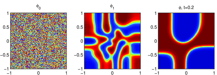
Figure 1: The two random initial values $\phi_{0}$, $\phi_{1}$ and the state of $\phi_{1}$ evolves $0.2$ time unit according to the Cahn-Hilliard equation (1.3) with $\gamma=1$.

4.1 Stability results

Table 1 shows the required minimum values of $A$ (resp. $B$) with different $\gamma$, $B$ (resp. $A$) and $\tau$ values for stably solving (not blow up in 4096 time steps) the Cahn-Hilliard equation (1.3) with initial value $\phi_{0}$. The results for the initial value $\phi_{1}$ are similar. From this table, we observe that the SL-CN scheme is stable with $A=0,B=0$ when $\tau$ is small enough. If we take $A=0$, then $B=16$ will make the scheme unconditionally stable, the values of $\gamma$ has only a very small effect on the values of $B$. But when we fix $B$, the case $\gamma=1$ requires a much larger $A$ value to make the scheme stable than $\gamma=0.0025$ case, this is consistent to our analysis.

$\tau$	Minimum A required				Minimum B required
	$\gamma=0.0025$		$\gamma=1$		$\gamma=0.0025$		$\gamma=1$
	$B=0$	$B=10$	$B=0$	$B=10$	$A=0$	$A=4$	$A=0$	$A=4$
10	0.16	0.005	1	1	16	8	16	0
1	0.16	0	8	1	16	16	16	2
0.1	0.16	0	32	1	8	4	16	8
0.01	0.08	0	64	2	8	4	16	8
0.001	0	0	64	0	0	0	8	8
0.0001	0	0	64	0	0	0	8	4
1E-05	0	0	32	0	0	0	2	2
1E-06	0	0	0	0	0	0	0	0

Table 1: The minimum values of $A$(resp $B$) (only values $\{0,2^{i},i=0,\ldots,7\}\times\gamma$ are tested for $A$, only values $\{0,2^{i},i=0,\ldots,7\}$ are tested for $B$) to make scheme SL-CN stable when $\gamma$, $B$ (resp $A$) and $\tau$ taking different values.

Figure 2 presents the discrete energy dissipation of the SL-CN scheme using several time step-sizes. We see clearly the energy decaying property is maintained. Moreover, as $t$ increases, the differences between $E$ and $E_{CN}$ get smaller and smaller.

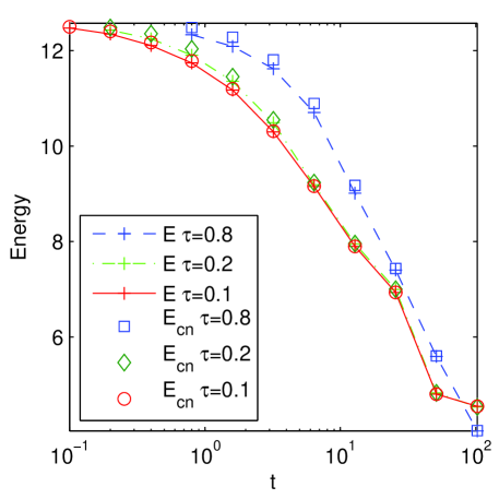
Figure 2: The discrete energy dissipation of the SL-CN scheme solving the Cahn-Hilliard equation with initial value $\phi_{1}$, and relaxation parameter $\gamma=0.0025$. Stability constant $A=1,B=20$ are used.

4.2 Accuracy results

We take initial value $\phi_{1}$ to test the accuracy of the two schemes. The Cahn-Hilliard equation with $\gamma=0.0025$ are solved from $t=0$ to $T=12.8$. To calculate the numerical error, we use the numerical result generated using $\tau=10^{-3}$ as a reference of exact solution. The results are given in Table 2. We see that the scheme is second order accuracy in $H^{-1},L^{2}$ and $H^{1}$ norm.

$\tau$	$H^{-1}$ Error	Order	$L^{2}$ Error	Order	$H^{1}$ Error	Order
0.16	7.98E-02		5.20E-01		6.40E+00
0.08	2.18E-02	1.87	1.64E-01	1.66	2.18E+00	1.56
0.04	5.95E-03	1.87	4.57E-02	1.85	6.08E-01	1.84
0.02	1.54E-03	1.95	1.16E-02	1.97	1.55E-01	1.97
0.01	3.86E-04	2.00	2.90E-03	2.00	3.87E-02	2.00
0.005	9.38E-05	2.04	7.05E-04	2.04	9.39E-03	2.04

Table 2: The convergence of the SL-CN scheme with $B=40$, $A=0.1$ for the Cahn-Hilliard equation with initial value $\phi_{1}$,parameter $\gamma=0.0025$. The errors are calculated at $T=12.8$.

5 Conclusions

We study the stability and convergence of a stabilized linear Crank-Nicolson scheme for the Cahn-Hilliard phase field equation. The scheme includes two second-order stabilization terms, which guarantee the unconditional energy dissipation theoretically. Use a standard error analysis procedure for parabolic equation, we get an error estimate with a prefactor depending on $1/\varepsilon$ exponentially. We then refine the result by using a spectrum estimate of the linearized Cahn-Hilliard operator and mathematical induction to get an optimal (second-order) convergence estimate in $l^{\infty}(0,T;H^{-1})\cap l^{2}(0,T;H^{1})$ norm with a prefactor depends only on some lower degree polynomial of $1/\varepsilon$. Numerical results are presented to verify the stability and accuracy of the scheme.

References

References

ABC [94]
Nicholas D. Alikakos, Peter W. Bates, and Xinfu Chen.
Convergence of the Cahn-Hilliard equation to the Hele-Shaw
model.
Archive for Rational Mechanics and Analysis, 128(2):165–205,
June 1994.
AC [79]
S. M. Allen and J. W. Cahn.
A microscopic theory for antiphase boundary motion and its
application to antiphase domain coarsening.
Acta Metall. Mater., 27:1085–1095, 1979.
BBG [99]
J. Barrett, J. Blowey, and H. Garcke.
Finite element approximation of the Cahn-Hilliard equation with
degenerate mobility.
SIAM J. Numer. Anal., 37(1):286–318, 1999.
BMS [14]
B. Benesová, C. Melcher, and E. Süli.
An implicit midpoint spectral approximation of nonlocal
Cahn–Hilliard equations.
SIAM J. Numer. Anal., 52(3):1466–1496, 2014.
BZH+ [13]
A. Baskaran, P. Zhou, Z. Hu, C. Wang, S. Wise, and J. Lowengrub.
Energy stable and efficient finite-difference nonlinear multigrid
schemes for the modified phase field crystal equation.
J. Comput. Phys., 250:270–292, 2013.
CH [58]
John W. Cahn and John E. Hilliard.
Free energy of a nonuniform system. I. interfacial free energy.
J. Chem. Phys., 28(2):258–267, 1958.
Che [94]
Xinfu Chen.
Spectrum for the Allen-Cahn, Cahn-Hillard, and phase-field
equations for generic interfaces.
Commun. Part. Diff. Eq., 19(7):1371–1395, 1994.
CM [95]
Luis A. Caffarelli and Nora E. Muler.
An bound for solutions of the Cahn-Hilliard
equation.
Arch. Rational Mech. Anal., 133(2):129–144, 1995.
CMS [11]
Nicolas Condette, Christof Melcher, and Endre Süli.
Spectral approximation of pattern-forming nonlinear evolution
equations with double-well potentials of quadratic growth.
Math. Comp., 80(273):205–223, 2011.
CS [98]
L.Q. Chen and J. Shen.
Applications of semi-implicit Fourier-spectral method to phase
field equations.
Comput. Phys. Commun., 108(2-3):147–158, 1998.
CWWW [14]
W. Chen, C. Wang, X. Wang, and S.M. Wise.
A linear iteration algorithm for a second-order energy stable scheme
for a thin film model without slope selection.
J Sci. Comput., 59(3):574–601, 2014.
DN [91]
Qiang Du and Roy A. Nicolaides.
Numerical analysis of a continuum model of phase transition.
SIAM J Numer. Anal., 28(5):1310–1322, 1991.
DWW [16]
A. E. Diegel, C. Wang, and S. M. Wise.
Stability and convergence of a second order mixed finite element
method for the Cahn-Hilliard equation.
IMA J Numer. Anal., 36(4):1867–1897, 2016.
EG [96]
C. Elliott and H. Garcke.
On the Cahn-Hilliard Equation with Degenerate Mobility.
SIAM J Math. Anal., 27(2):404–423, 1996.
EL [92]
Charles M. Elliott and Stig Larsson.
Error estimates with smooth and nonsmooth data for a finite element
method for the Cahn-Hilliard equation.
Math. Comp., 58(198):603–630, S33–S36, 1992.
ES [93]
C. M. Elliott and A. M. Stuart.
The global dynamics of discrete semilinear parabolic equations.
SIAM J. Numer. Anal., 30:1622–1663, 1993.
Eyr [98]
D. J. Eyre.
Unconditionally gradient stable time marching the Cahn-Hilliard
equation.
In Computational and Mathematical Models of Microstructural
Evolution (San Francisco, CA, 1998), volume 529 of Mater. Res.
Soc. Sympos. Proc., pages 39–46. MRS, 1998.
Fen [06]
X. Feng.
Fully discrete finite element approximations of the
Navier-Stokes–Cahn-Hilliard diffuse interface model for two-phase
fluid flows.
SIAM J. Numer. Anal., 44(3):1049–1072, 2006.
FP [04]
Xiaobing Feng and Andreas Prohl.
Error analysis of a mixed finite element method for the
Cahn-Hilliard equation.
Numer. Math., 99(1):47–84, 2004.
FP [05]
Xiaobing Feng and Andreas Prohl.
Numerical analysis of the Cahn-Hilliard equation and
approximation of the Hele-Shaw problem.
Interfaces Free Bound, 7(1):1–28, 2005.
FTY [13]
Xinlong Feng, Tao Tang, and Jiang Yang.
Stabilized Crank-Nicolson/Adams-Bashforth schemes for phase
field models.
E Asian J Appl. Math., 3(1):59–80, 2013.
Fur [01]
Daisuke Furihata.
A stable and conservative finite difference scheme for the
Cahn-Hlliard equation.
Numer. Math., 87(4):675–699, 2001.
GGT [13]
F. Guillén-González and G. Tierra.
On linear schemes for a Cahn-Hilliard diffuse interface model.
J. Comput. Phys., 234:140–171, 2013.
GGT [14]
Francisco Guillén-González and Giordano Tierra.
Second order schemes and time-step adaptivity for Allen-Cahn and
Cahn-Hilliard models.
Comput. Math. Appl., 68(8):821–846, 2014.
GH [11]
Hector Gomez and Thomas J. R. Hughes.
Provably unconditionally stable, second-order time-accurate, mixed
variational methods for phase-field models.
J. Comput. Phys., 230(13):5310–5327, 2011.
GWWY [16]
Jing Guo, Cheng Wang, Steven M. Wise, and Xingye Yue.
An convergence of a second-order convex-splitting, finite
difference scheme for the three-dimensional Cahn-Hilliard equation.
Commun. Math. Sci, 14(2):489–515, 2016.
HBYT [17]
D. Han, A. Brylev, X. Yang, and Z. Tan.
Numerical analysis of second order, fully discrete energy stable
schemes for phase field models of two phase incompressible flows.
J. Sci. Comput., 70:965–989, 2017.
HLT [07]
Yinnian He, Yunxian Liu, and Tao Tang.
On large time-stepping methods for the Cahn-Hilliard equation.
Appl. Numer. Math., 57(5-7):616–628, 2007.
KKL [04]
Junseok Kim, Kyungkeun Kang, and John Lowengrub.
Conservative multigrid methods for Cahn-Hilliard fluids.
J. Comput. Phys., 193(2):511–543, 2004.
KNS [04]
Daniel Kessler, Ricardo H. Nochetto, and Alfred Schmidt.
A posteriori error control for the Allen-Cahn problem:
circumventing Gronwall’s inequality.
ESAIM: Math. Model. Numer. Anal., 38(01):129–142, 2004.
LQ [17]
Dong Li and Zhonghua Qiao.
On second order semi-implicit Fourier spectral methods for 2d
Cahn-Hilliard equations.
J Sci. Comput., 70(1):301–341, 2017.
LQT [16]
Dong Li, Zhonghua Qiao, and Tao Tang.
Characterizing the stabilization size for semi-implicit
Fourier-spectral method to phase field equations.
SIAM J Numer. Anal., 54(3):1653–1681, 2016.
LS [03]
Chun Liu and Jie Shen.
A phase field model for the mixture of two incompressible fluids and
its approximation by a Fourier-spectral method.
Physica D, 179(3-4):211–228, 2003.
MPC+ [13]
F Magaletti, Francesco Picano, M Chinappi, Luca Marino, and Carlo Massimo
Casciola.
The sharp-interface limit of the Cahn–Hilliard/Navier–Stokes
model for binary fluids.
J Fluid. Mech., 714:95–126, 2013.
SY [10]
Jie Shen and Xiaofeng Yang.
Numerical approximations of Allen-Cahn and Cahn-Hilliard
equations.
Discrete Cont. Dyn. A, 28:1669–1691, 2010.
SYY [15]
Jie Shen, Xiaofeng Yang, and Haijun Yu.
Efficient energy stable numerical schemes for a phase field moving
contact line model.
J. Comput. Phys., 284:617–630, 2015.
WvZvdZ [14]
X. Wu, G. J. van Zwieten, and K. G. van der Zee.
Stabilized second-order convex splitting schemes for
Cahn-Hilliard models with application to diffuse-interface tumor-growth
models.
Int. J. Numer. Meth. Biomed. Engng., 30(2):180–203, 2014.
WY [17]
Lin Wang and Haijun Yu.
Two efficient second order stabilized semi-implicit schemes for the
Cahn-Hilliard phase-field equation.
arXiv:1708.09763 [math], August 2017.
XT [06]
C. Xu and T. Tang.
Stability analysis of large time-stepping methods for epitaxial
growth models.
SIAM J. Num. Anal., 44:1759–1779, 2006.
Yan [16]
Xiaofeng Yang.
Linear, first and second-order, unconditionally energy stable
numerical schemes for the phase field model of homopolymer blends.
J. Comput. Phys., 327:294–316, 2016.
YJ [17]
Xiaofeng Yang and Lili Ju.
Efficient linear schemes with unconditional energy stability for the
phase field elastic bending energy model.
Comput. Method. Appl. Mech. Eng., 315:691–712, 2017.
YY [17]
Xiaofeng Yang and Haijun Yu.
Efficient second order energy stable schemes for a phase-field moving
contact line model.
arXiv:1703.01311, 2017.
YZWS [17]
X. Yang, J. Zhao, Q. Wang, and J. Shen.
Numerical approximations for a three components Cahn-Hilliard
phase-field model based on the invariant energy quadratization method.
Math. Models Methods Appl. Sci., 27:1993, 2017.
ZCST [99]
Jingzhi Zhu, Long-Qing Chen, Jie Shen, and Veena Tikare.
Coarsening kinetics from a variable-mobility Cahn-Hilliard
equation: Application of a semi-implicit Fourier spectral method.
Phys. Rev. E, 60(4):3564–3572, 1999.
ZMQ [13]
Zhengru Zhang, Yuan Ma, and Zhonghua Qiao.
An adaptive time-stepping strategy for solving the phase field
crystal model.
J. Comput. Phys., 249:204–215, 2013.