The design of conservative finite element discretisations for the vectorial modified KdV equation

Abstract.

We design a consistent Galerkin scheme for the approximation of the vectorial modified Korteweg-de Vries equation. We demonstrate that the scheme conserves energy up to machine precision. In this sense the method is consistent with the energy balance of the continuous system. This energy balance ensures there is no numerical dissipation allowing for extremely accurate long time simulations free from numerical artifacts. Various numerical experiments are shown demonstrating the asymptotic convergence of the method with respect to the discretisation parameters. Some simulations are also presented that correctly capture the unusual interactions between solitons in the vectorial setting.

1. Introduction

Hamiltonian partial differential equations (PDEs) are a specific class of PDE endowed with physically relevant algebraic and geometric structures [Olv93]. They arise form a variety of areas [She90], not least meteorological, such as the semi-geostrophic equations [RN94], and oceanographical, such as the Korteweg-de Vries (KdV) and nonlinear Schrödinger equations [MGO05]. The KdV and nonlinear Schrödinger equations are particularly special examples, in that they are bi-Hamiltonian [Mag78]. This means they have two different Hamiltonian formulations which, in turn, is one way to understand the notion of integrability of these problems. Regardless, the applications and the need to quantify the dynamics of the general Cauchy problem motivate the development of accurate long time simulations for reliable prediction of dynamics in both meteorology and oceanography.

A difficulty in the design of schemes for this class of problems is that the long term dynamics of solutions can be destroyed by the addition of artificial numerical diffusion. The reason for inclusion of this in a given scheme is the desirable stability properties this endows on the approximation, however, this typically destroys all information in the long term dynamics of the system through smearing of solutions.

Conservative schemes for Hamiltonian ordinary differential equations (ODEs) are relatively well understood, see [CGM⁺12, LR04, HLW06, BL07, BC16, c.f.]. Typically numerical schemes designed for this class of problem which have some property of the ODE built into them, for example conservativity of the Hamiltonian or the underlying symplectic form, are classified as geometric integrators. In the PDE setting symplectic structure preserving algorithms have also been developed [Rei00, BR01, COR08, CMR14]. Here the PDEs are rewritten using their corresponding symplectic form, and the notion of structure preservation is given in terms of a discrete (difference) conservation law involving differential forms. Typically these problems are solved using an Euler/Preissman box scheme, although space-time finite element methods under an appropriate quadrature choice form a natural generalisation.

In this contribution we consider a system of equations that are a multidimensional generalisation of the famous modified KdV equation

$$u_{t}+\frac{3}{2}u^{2}u_{x}+u_{xxx}=0,$$

where the subindices denote partial differentiation with respect to the corresponding independent variable. This equation has numerous applications not least including fluid dynamics and plasma physics [AC91]. The vectorial equation [MBSW02] appears frequently in the study of ocean waves and Riemannian geometry [SW03, ANW11, Anc06]. The presence of the Korteweg third order term as well as the lack of sign in the corresponding energy functional, further details given in §2, can cause issues in the numerical treatment of this problem. The vectorial equation also has additional complications that do not arise in the scalar setting. Indeed, the underlying conservation laws themselves have a vastly different structure, for example there is no mass conservation in the vectorial case. This is due to the different form of Hamiltonian operator.

In previous numerical studies of the scalar KdV and modified KdV equations [XS07, YS02, c.f.], it has been observed that classical finite volume and discontinuous Galerkin (dG) schemes with “standard” numerical fluxes introduce numerical artifacts. These typically appear through numerical regularisation effects included for stability purposes that are not, however, adapted to the variational structure of the problem. The result of these artifacts is an inconsistency in the discrete energy.

Hamiltonian problems are inherently conservative, that is, the underlying Hamiltonian is conserved over time. Other equations, including those of integrable type, may have additional structures that manifest themselves through additional conserved quantities. In particular, mass and momentum are such quantities. In [BCKX13] and [KM15] the authors propose and analyse a dG scheme for generalised KdV equations. The scheme itself is very carefully designed to be conservative, in that the invariant corresponding to the momentum is inherited by the discretisation. This yields $\operatorname{L}^{2}$ stability quite naturally in the numerical scheme and extremely good long time dynamics. In the scalar case one may also design schemes that conserve the energy itself [Win80, JP17], however, it does not seem possible to design schemes to conserve more than two of these invariants. A natural question is then “conservation of which invariant yields the best scheme?” [Jac17b].

When examining the case of systems of Hamiltonian equations much less work has been carried out, for example [BZ09] give a near conservative method for a system of Schrödinger–KdV type and [BDM07] study a system of KdV equations. To the authors knowledge there has not been any work on the system we study, nor such Hamiltonian systems in general. Our goal in this work is the derivation of Galerkin discretisations aimed at preserving the underlying algebraic properties satisfied by the PDE system whilst avoiding the introduction of stabilising diffusion terms. Our schemes are therefore consistent with (one of) the Hamiltonian formulation of the original problem. It is important to note that our approach is not an adaptation of entropy conserving schemes developed for systems of conservation laws, rather we study the algebraic properties of the PDE and formulate the discretisation to inherit this specific structure. The methods are of arbitrarily high order of accuracy in space and provide relevant approximations free from numerical artifacts. To the authors knowledge this is the first class of finite element method for this particular class of system to have these properties.

The rest of this work is set out as follows: In §2 we introduce notation, the model problem and some of its properties. We give a reformulation of the system through the introduction of auxiliary variables, these are introduced to allow for a simple construction of the numerical scheme. In §3 we examine a temporal discretisation of the problem that guarantees the conservation of the underlying Hamiltonian. In §4 we propose a spatial discretisation based on continuous finite elements, state a fully discrete method and show that it is conservative. Finally in §5 we summarise extensive numerical experiments aimed at testing the robustness of the method in long time simulations.

2. The vectorial modified KdV equation

In this section we formulate the model problem, fix notation and give some basic assumptions. We describe some known results and history of the vectorial modified Korteweg-de Vries (vmKdV) equation, highlighting the Hamiltonian structure of the equation. We show that the underlying Hamiltonian structure naturally yields an induced stability of the solutions to the PDE system and give a brief description of how to construct some exact solutions using a dressing method. We then show how the system can be written through induced auxiliary variables which are the basis of the design of our numerical scheme.

Throughout this work we denote the standard Lebesgue spaces by $\operatorname{L}^{p}(\omega)$ for $\omega\subseteq\mathbb{R}$, $p\in[1,\infty]$, equipped with corresponding norms $\left\|u\right\|_{\operatorname{L}^{p}(\omega)}$. In addition, we will denote $\operatorname{H}^{k}(\omega)$ to be the Hilbert space of order $k$ of real-valued functions defined over $\omega\subseteq\mathbb{R}$ with norm $\left\|u\right\|_{\operatorname{H}^{k}(\omega)}$.

The vmKdV equation is an evolutionary PDE for a real, $d$-vector valued function

(2.1) $$\begin{array}[]{rccl}{\boldsymbol{u}}:&{\mathbb{R}^{2}}&\to&{\mathbb{R}^{d}}\\ &{(x,t)}&\mapsto&{\boldsymbol{u}(x,t)={\!\left({u_{1}\dots,u_{d}}\right)}^{{\boldsymbol{\intercal}}}}\end{array}\quad$$

and is given by

(2.2) $$\boldsymbol{u}_{t}+\frac{3}{2}{\boldsymbol{u}}\cdot{\boldsymbol{u}}\boldsymbol{u}_{x}+\boldsymbol{u}_{xxx}=\boldsymbol{0}.$$

Here we are using “$\boldsymbol{x}\cdot\boldsymbol{y}$” as the Euclidean inner product between two vectors, $\boldsymbol{x}$ and $\boldsymbol{y}$ and “$\left|\boldsymbol{x}\right|$” as the induced Euclidean norm of $\boldsymbol{x}$.

A particular case of the vmKdV system occurs when $d=2$, $\boldsymbol{u}={\!\left({u_{1},u_{2}}\right)}^{{\boldsymbol{\intercal}}}$ when (2.2) can be identified with the complex modified KdV (mKdV) equation

(2.3) $$y_{t}+\frac{3}{2}\left|y\right|^{2}y_{x}+y_{xxx}=0$$

for the complex dependent variable $y=u_{1}+iu_{2}$. Sometimes this is also called the Hirota mKdV equation [Hir73]. When $d=1$ we obtain the famous mKdV equation which has been studied numerically in the context of Galerkin methods in [BCKX13, JP17].

Equation (2.2) admits both Lie and discrete point symmetries and has infinitely many conservation laws. Indeed, under the action of the orthogonal group $O_{d}(\mathbb{R})$, which is the group of $d\times d$ matrices such that ${\boldsymbol{A}}^{{\boldsymbol{\intercal}}}\boldsymbol{A}=\operatorname{\bf I}$,

(2.4) $$\widetilde{\boldsymbol{u}}=\boldsymbol{A}\boldsymbol{u},\quad\text{ for }\boldsymbol{A}\in O_{d}(\mathbb{R})$$

equation (2.2) remains invariant. Moreover, vmKdV is invariant under the translations

(2.5) $$\widetilde{x}=x+\epsilon,\quad\widetilde{t}=t+\gamma$$

and under the scaling transformation

(2.6) $$\left(\widetilde{x},\widetilde{t},\widetilde{\boldsymbol{u}}\right)=\left(e^{\epsilon}x,e^{3\epsilon}t,e^{-\epsilon}\boldsymbol{u}\right).$$

2.1 Proposition (Conservative properties of solutions).

The vmKdV equation admits the following conservation laws:

(2.7) $$\begin{split}\mathrm{D}_{t}f_{2}(\boldsymbol{u})&=\mathrm{D}_{x}g_{2}(\boldsymbol{u})\\ \mathrm{D}_{t}f_{4}(\boldsymbol{u})&=\mathrm{D}_{x}g_{4}(\boldsymbol{u}),\end{split}$$

where the conserved densities are given by

(2.8) $$\begin{split}f_{2}(\boldsymbol{u})&=\frac{1}{2}\left|\boldsymbol{u}\right|^{2}\\ f_{4}(\boldsymbol{u})&=\frac{1}{2}\left|\boldsymbol{u}_{x}\right|^{2}-\frac{1}{8}\left|\boldsymbol{u}\right|^{4}\end{split}$$

and the corresponding fluxes are

(2.9) $$\begin{split}g_{2}(\boldsymbol{u})&=\left|\boldsymbol{u}_{x}\right|^{2}-2\boldsymbol{u}\cdot\boldsymbol{u}_{xx}-\frac{3}{4}\left|\boldsymbol{u}\right|^{4}\\ g_{4}(\boldsymbol{u})&=\frac{1}{8}\left|\boldsymbol{u}\right|^{6}-\left|\boldsymbol{u}\right|^{2}\left|\boldsymbol{u}_{x}\right|^{2}-\frac{1}{2}\!\left({\boldsymbol{u}\cdot\boldsymbol{u}_{x}}\right)^{2}-\boldsymbol{u}_{x}\cdot\boldsymbol{u}_{xxx}+\frac{1}{2}\left|\boldsymbol{u}_{xx}\right|^{2}+\frac{1}{2}\left|\boldsymbol{u}\right|^{2}\boldsymbol{u}\cdot\boldsymbol{u}_{xx}.\end{split}$$

Proof To prove that the total time derivative of $f_{2}(\textbf{u})$ and $f_{4}(\textbf{u})$ are in the image of $D_{x}$ we use the Euler operator $\boldsymbol{E}=(E_{1},...,E_{d})$, where

$$E_{i}(f)=\sum_{k=0}^{\infty}(-D_{x})^{k}\partial_{u_{i_{kx}}}f,\quad u_{i_{kx}}=u_{i_{\underbrace{x...x}_{k}}}$$

and the fact that $\text{Ker}\boldsymbol{E}=\text{Im}D_{x}$, see [Olv93] for a proof. On the other hand in order to calculate the corresponding fluxes $g_{2}$ and $g_{4}$ we apply the homotopy operator [Olv93] to $D_{t}f_{2}(\textbf{u})$ and $D_{t}f_{4}(\textbf{u})$ respectively. The homotopy operator is given by

$$H(f(\textbf{u}))=\int_{0}^{1}\sum_{i=1}^{d}\text{I}_{i}(f)(\lambda\textbf{u})\frac{d\lambda}{\lambda}$$

where

$$\text{I}_{i}(f)=\sum_{k=1}^{\infty}\left(\sum_{s=0}^{k-1}u_{i_{sx}}(-D_{x})^{k-s-1}\right)f_{u_{i_{kx}}}.$$

∎

2.2 Corollary.

Let $\mathbb{S}^{1}$ be the unitary circle, i.e., $[0,1]$ with matching endpoints. Then from Proposition 2.1 it follows that, upon defining

(2.10) $$F_{2}(\boldsymbol{u}):=\int_{\mathbb{S}^{1}}f_{2}(\boldsymbol{u})\,\mathrm{d}x$$

as the momentum functional and

(2.11) $$F_{4}(\boldsymbol{u}):=\int_{\mathbb{S}^{1}}f_{4}(\boldsymbol{u})\,\mathrm{d}x$$

as the energy functional for periodic solutions we have

(2.12) $$\mathrm{D}_{t}F_{2}(\boldsymbol{u})=\mathrm{D}_{t}F_{4}(\boldsymbol{u})=0.$$

Moreover this does not just hold for periodic solutions over $\mathbb{S}^{1}$. Indeed, one can consider the equation (2.2) over $\mathbb{R}$ and require that solutions decay at infinity, for example Schwartz functions, and the result holds. A particular example of these are the much celebrated soliton solutions. The conservation laws also allow for the a priori control of the solution.

2.3 Proposition (Stability bound).

Let the vmKdV system (2.2), defined over $\mathbb{S}^{1}$, be coupled with initial conditions $\boldsymbol{u}_{0}$ satisfying $F_{2}(\boldsymbol{u}_{0})=C_{2}<\infty$ and $F_{4}(\boldsymbol{u}_{0})=C_{4}<\infty$ then $\boldsymbol{u}$ satisfies

(2.13) $$\left\|\boldsymbol{u}_{x}(t)\right\|_{\operatorname{L}^{2}(\mathbb{S}^{1})}\leq\!\left({4C_{4}+\frac{C_{GN}^{8}C_{2}^{3}}{2}}\right)^{1/2},$$

where $C_{GN}$ is a constant appearing from the Gagliardo-Nirenberg interpolation inequality.

Proof In view of the definition of $F_{4}(\boldsymbol{u})$ we have that

(2.14) $$\begin{split}\left\|\boldsymbol{u}_{x}\right\|_{\operatorname{L}^{2}(\mathbb{S}^{1})}^{2}&=2F_{4}(\boldsymbol{u})+\frac{1}{4}\left\|\boldsymbol{u}\right\|_{\operatorname{L}^{4}(\mathbb{S}^{1})}^{4}\\ &=2F_{4}(\boldsymbol{u}_{0})+\frac{1}{4}\left\|\boldsymbol{u}\right\|_{\operatorname{L}^{4}(\mathbb{S}^{1})}^{4},\end{split}$$

through the conservativity of $F_{4}(\boldsymbol{u})$ given in Theorem 2.1. Now making use of the Gagliardo-Nirenberg interpolation inequality there exists a constant $C_{GN}$ such that

(2.15) $$\left\|\boldsymbol{u}\right\|_{\operatorname{L}^{4}(\mathbb{S}^{1})}\leq C_{GN}\left\|\boldsymbol{u}\right\|_{\operatorname{L}^{2}(\mathbb{S}^{1})}^{3/4}\left\|\boldsymbol{u}_{x}\right\|_{\operatorname{L}^{2}(\mathbb{S}^{1})}^{1/4},$$

hence

(2.16) $$\begin{split}\frac{1}{4}\left\|\boldsymbol{u}\right\|_{\operatorname{L}^{4}(\mathbb{S}^{1})}^{4}&\leq\frac{1}{4}C_{GN}^{4}\left\|\boldsymbol{u}\right\|_{\operatorname{L}^{2}(\mathbb{S}^{1})}^{3}\left\|\boldsymbol{u}_{x}\right\|_{\operatorname{L}^{2}(\mathbb{S}^{1})}\\ &\leq\frac{1}{32}C_{GN}^{8}{\left\|\boldsymbol{u}\right\|_{\operatorname{L}^{2}(\mathbb{S}^{1})}^{6}}+\frac{1}{2}{\left\|\boldsymbol{u}_{x}\right\|_{\operatorname{L}^{2}(\mathbb{S}^{1})}^{2}},\end{split}$$

through Young’s inequality. Substituting (2.16) into (2.14) we see

(2.17) $$\begin{split}\frac{1}{2}\left\|\boldsymbol{u}_{x}\right\|_{\operatorname{L}^{2}(\mathbb{S}^{1})}^{2}&\leq 2F_{4}(\boldsymbol{u}_{0})+\frac{C_{GN}^{8}}{32}\left\|\boldsymbol{u}\right\|_{\operatorname{L}^{2}(\mathbb{S}^{1})}^{6}\\ &\leq 2F_{4}(\boldsymbol{u}_{0})+\frac{C_{GN}^{8}}{4}F_{2}(\boldsymbol{u})^{3}\\ &\leq 2F_{4}(\boldsymbol{u}_{0})+\frac{C_{GN}^{8}}{4}F_{2}(\boldsymbol{u}_{0})^{3}\\ &\leq 2C_{4}+\frac{C_{GN}^{8}C_{2}^{3}}{4},\end{split}$$

using the conservativity of $F_{2}(\boldsymbol{u})$, concluding the proof. ∎

2.4 Remark (Hierarchy of conservation laws).

Note that the vmKdV equation (2.2) admits an infinite hierarchy of conserved quantities. For example, after $F_{2}(\boldsymbol{u})$ and $F_{4}(\boldsymbol{u})$ the next member of the hierarchy is

(2.18) $$F_{6}(\boldsymbol{u})=\int_{{S}^{1}}\frac{1}{2}\left|\boldsymbol{u}\right|^{6}+10\!\left({\boldsymbol{u}\cdot\boldsymbol{u}_{x}}\right)^{2}+\left|\boldsymbol{u}\right|^{2}\left|\boldsymbol{u}_{x}\right|^{2}+7\left|\boldsymbol{u}\right|^{2}\!\left({\boldsymbol{u}\cdot\boldsymbol{u}_{xx}}\right)+4\left|\boldsymbol{u}_{xx}\right|^{2}\,\mathrm{d}x.$$

A generating function of the conserved densities for the vmKdV is constructed using its Lax representation in [AP17].

Together with the Gagliardo-Nirenberg interpolation inequality one may derive a priori bounds of a similar form to that given in Theorem 2.3 but in higher order norms. Indeed, for $s\in\mathbb{N}$ the conservation law $F_{2s}$ naturally gives rise to a stability bound in $\operatorname{H}^{s-1}$.

2.5. Exact solutions to the vmKdV system

The vmKdV equation (2.2) is integrable and has already drawn some attention [AP17, ANW11]. Its integrability properties were derived using the structure equation for the evolution of a curve embedded in an $n$-dimensional Riemannian manifold with constant curvature [SW03, Anc06, MBSW02]. The associated Cauchy problem can be studied analytically using the inverse scattering transform [AC91, NMPZ84, FT07]. Due to the fact that it admits a zero curvature representation (or a Lax representation, see [Lax76, c.f.]), i.e., it can be written in the following form:

(2.19) $$U_{t}-V_{x}+\left[U,V\right]=0,$$

where $U=U(\boldsymbol{u};\lambda)$ and $V=V(\boldsymbol{u};\lambda)$ are appropriate matrices in a Lie algebra having a polynomial dependence on a spectral parameter $\lambda\in\mathbb{C}$. One can construct, see [AP17], a Darboux matrix $M$ [RS02, SM91] that maps the pair $(U,V)$ to

(2.20) $$(U,V)\mapsto(\widetilde{U},\widetilde{V})=(MUM^{-1}+M_{x}M^{-1},MUM^{-1}+M_{t}M^{-1})$$

and $\widetilde{U}=U(\widetilde{\boldsymbol{u}};\lambda)$ and $\widetilde{V}=V(\widetilde{\boldsymbol{u}};\lambda)$. In other words $\widetilde{U}$ and $\widetilde{V}$ have the same structure as $U$ and $V$ respectively. The transformation (2.20) implies a nonlocal symmetry $\boldsymbol{u}\mapsto\widetilde{\boldsymbol{u}}$ of the vmKdV, known as a Bäcklund transformation. Such transformations that have applications in geometry [RS02] are characteristic of integrable equations. Starting with the trivial background solution $\boldsymbol{u}=\boldsymbol{0}$ one can then recursively and algebraically construct the soliton solutions of vmKdV equation (2.2). For example, when $d=2$ a 1-soliton solution is given by

(2.21) $$\boldsymbol{u}=\frac{2\mu}{\cosh\xi_{\mu}}\boldsymbol{E},$$

where $\mu\in\mathbb{R}$, $\xi_{\mu}=\mu\!\left({x-c_{\mu}}\right)-\mu^{3}t$, for some shift $c_{\mu}\in\mathbb{R}$ and $\boldsymbol{E}$ is a constant unit vector. A 2-soliton solution is given by

(2.22) $$\boldsymbol{u}=\frac{F_{\mu,\nu}}{G}\boldsymbol{E}_{1}+\frac{F_{\nu,\mu}}{G}\boldsymbol{E}_{2},$$

where $\boldsymbol{E}_{1}$ and $\boldsymbol{E}_{2}$ are constant unit vectors, $\mu,~{}\nu\in\mathbb{R}$ with $\mu\neq\pm\nu$ and

(2.23) $$F_{k,l}=2(l^{2}-k^{2})l\cosh\xi_{k}$$

and

(2.24) $$G=(\mu^{2}+\nu^{2})\cosh\xi_{\mu}\cosh\xi_{\nu}-2\mu\nu\sinh\xi_{\mu}\sinh\xi_{\nu}-2\mu\nu\boldsymbol{E}_{1}\cdot\boldsymbol{E}_{2}.$$

The 1-soliton (2.21) and 2-soliton (2.22) solutions, while elegant, are not the most general of their kind, see [AP17] for details. Nevertheless, the exact solutions (2.21) and (2.22) are both perfectly adequate for benchmarking our scheme which we shall use them for in §5. Such solutions can also be derived using Hirota’s bilinear form [Hir04, ANW11].

Solitons are, however, a special class of solution for this problem with a very particular structure. In general one cannot write down closed form solutions for this problem motivating the need for long time accurate numerical schemes. We shall proceed by describing the Hamiltonian structure of the vmKdV problem which forms the basis for the design of our numerical scheme.

2.6 Remark (Problem reformulation and motivation).

Since the vmKdV system is Hamiltonian it can be written as

(2.25) $$\boldsymbol{u}_{t}=\mathscr{P}(\boldsymbol{u})\frac{\delta F_{4}(\boldsymbol{u})}{\delta\boldsymbol{u}},$$

where $\mathscr{P}(\boldsymbol{u})$ is a Hamiltonian operator, $F_{4}(\boldsymbol{u})$ is the induced Hamiltonian and $\frac{\delta\cdot}{\delta\boldsymbol{u}}$ denotes the first variation with respect to $\boldsymbol{u}$ [Olv93]. For this specific problem the Hamiltonian operator acts on a real, $d$-vector function $\boldsymbol{y}$ and takes the form [Anc06]

(2.26) $$\begin{split}\mathscr{P}(\boldsymbol{u})\boldsymbol{y}:=\boldsymbol{y}_{x}+\boldsymbol{u}\bigg{\lrcorner}\!\left[{\mathrm{D}_{x}^{-1}\!\left({\boldsymbol{y}\otimes\boldsymbol{u}-\boldsymbol{u}\otimes\boldsymbol{y}}\right)}\right],\end{split}$$

where $\mathrm{D}_{x}^{-1}$ is the formal inverse operator of $\mathrm{D}_{x}$, $\otimes$ is the tensor product between vectors and $\lrcorner$ is an interior product defined through

(2.27) $$\boldsymbol{x}\lrcorner\!\left({\boldsymbol{y}\otimes\boldsymbol{z}}\right)=\!\left({\boldsymbol{x}\cdot\boldsymbol{y}}\right)\boldsymbol{z}.$$

This then induces a Poisson bracket

(2.28) $$\{F,G\}:=\int_{\mathbb{R}}\frac{\delta F}{\delta u}\mathscr{P}(\boldsymbol{u})\frac{\delta G}{\delta u}\,\mathrm{d}x,$$

a skew-symmetric bilinear form satisfying the Jacobi identity. In view of the skew-symmetry of $\mathscr{P}(\boldsymbol{u})$ we have

(2.29) $$\mathrm{D}_{t}F_{4}(\boldsymbol{u})=\{F_{4}(\boldsymbol{u}),F_{4}(\boldsymbol{u})\}=0.$$

Notice also that the vmKdV system can also be written as

(2.30) $$\boldsymbol{u}_{t}=\{\boldsymbol{u},F_{4}(\boldsymbol{u})\}.$$

The main idea behind the discretisation we propose is to correctly represent the Hamiltonian operator in the finite element space whilst preserving the skew-symmetry property of the underlying bracket. Indeed, the proof of Proposition 2.1 motivates rewriting the vmKdV system by introducing auxiliary variables to represent different components of the Hamiltonian operator. We consider seeking the tuple $\!\left({\boldsymbol{u},\boldsymbol{v},\boldsymbol{w}}\right)$ such that

(2.31) $$\begin{split}\boldsymbol{0}&=\boldsymbol{u}_{t}+\boldsymbol{v}_{x}+\boldsymbol{w}\\ \boldsymbol{0}&=\boldsymbol{v}-\frac{1}{2}\left|\boldsymbol{u}\right|^{2}\boldsymbol{u}-\boldsymbol{u}_{xx}\\ \boldsymbol{0}&=\boldsymbol{w}-\left|\boldsymbol{u}\right|^{2}\boldsymbol{u}_{x}+\!\left({\boldsymbol{u}_{x}\cdot\boldsymbol{u}}\right)\boldsymbol{u}.\end{split}$$

Notice that $\boldsymbol{v}=\frac{\delta F_{4}(\boldsymbol{u})}{\delta u}$ and $\boldsymbol{w}=\boldsymbol{u}\bigg{\lrcorner}\!\left[{\mathrm{D}_{x}^{-1}\!\left({\boldsymbol{v}\otimes\boldsymbol{u}-\boldsymbol{u}\otimes\boldsymbol{v}}\right)}\right]$. This form of $\boldsymbol{w}$ is extremely important as the Hamiltonian operator given in (2.26) is nonlocal. The fact that it can be “localised” by removing the $\mathrm{D}_{x}^{-1}$ allows for the efficient approximation by Galerkin methods.

This reformulation also means that in the case both arguments of the Poisson bracket are the Hamiltonian we may write

(2.32) $$0=\{F_{4}(\boldsymbol{u}),F_{4}(\boldsymbol{u})\}=\int_{\mathbb{R}}\boldsymbol{v}\cdot\!\left({\boldsymbol{v}_{x}+\boldsymbol{w}}\right)\,\mathrm{d}x.$$

It is exactly this structure that we try to exploit.

2.7 Remark (Relation to the scalar case).

As already mentioned when $d=1$, the problem reduces to the mKdV equation. In this case $w\equiv 0$ and the mixed system coincides with that proposed in [JP17]. Energy conservative schemes can be derived and proven to converge using the same techniques presented in that work. For $d>1$, $\boldsymbol{w}$ is not necessarily zero and represents the additional contribution arising from the Hamiltonian operator described in Remark 2.6.

2.8 Proposition (The mixed system is conservative).

Let $\boldsymbol{u},\boldsymbol{v},\boldsymbol{w}$ be given by (2.31) then we have that

(2.33) $$\mathrm{D}_{t}F_{4}(\boldsymbol{u})=\mathrm{D}_{t}\int_{\mathbb{S}^{1}}\frac{1}{2}\left|\boldsymbol{u}_{x}\right|^{2}-\frac{1}{8}\left|\boldsymbol{u}\right|^{4}\,\mathrm{d}x=0.$$

Proof Since the mixed system is equivalent to the vmKdV system the proof is clear through Proposition 2.1, however, for illustrative purposes we present it in full as it will become the basis for the design of our numerical scheme. To begin note

(2.34) $$\begin{split}\mathrm{D}_{t}F_{4}(\boldsymbol{u})&=\int_{\mathbb{S}^{1}}\boldsymbol{u}_{x}\cdot\boldsymbol{u}_{xt}-\frac{1}{2}\left|\boldsymbol{u}\right|^{2}\boldsymbol{u}\cdot\boldsymbol{u}_{t}\,\mathrm{d}x\\ &=\int_{\mathbb{S}^{1}}-\boldsymbol{u}_{xx}\cdot\boldsymbol{u}_{t}-\frac{1}{2}\left|\boldsymbol{u}\right|^{2}\boldsymbol{u}\cdot\boldsymbol{u}_{t}\,\mathrm{d}x\\ &=\int_{\mathbb{S}^{1}}-\boldsymbol{v}\cdot\boldsymbol{u}_{t}\,\mathrm{d}x.\end{split}$$

Now making use of (2.31)

(2.35) $$\begin{split}\mathrm{D}_{t}F_{4}(\boldsymbol{u})&=\int_{\mathbb{S}^{1}}\boldsymbol{v}\cdot\!\left({\boldsymbol{v}_{x}+\boldsymbol{w}}\right)\,\mathrm{d}x\\ &=\int_{\mathbb{S}^{1}}\boldsymbol{v}\cdot\boldsymbol{w}\,\mathrm{d}x\\ &=\int_{\mathbb{S}^{1}}\!\left({\frac{1}{2}\left|\boldsymbol{u}\right|^{2}\boldsymbol{u}+\boldsymbol{u}_{xx}}\right)\cdot\boldsymbol{w}\,\mathrm{d}x.\end{split}$$

Note that from (2.31) we can see that $\boldsymbol{w}\cdot\boldsymbol{u}=0$ and hence

(2.36) $$\begin{split}\mathrm{D}_{t}F_{4}(\boldsymbol{u})&=\int_{\mathbb{S}^{1}}\boldsymbol{u}_{xx}\cdot\boldsymbol{w}\,\mathrm{d}x\\ &=\int_{\mathbb{S}^{1}}\boldsymbol{u}_{xx}\cdot\!\left({\left|\boldsymbol{u}\right|^{2}\boldsymbol{u}_{x}-\!\left({\boldsymbol{u}_{x}\cdot\boldsymbol{u}}\right)\boldsymbol{u}}\right)\,\mathrm{d}x.\end{split}$$

Now, through an integration by parts we have

(2.37) $$\begin{split}\int_{\mathbb{S}^{1}}\left|\boldsymbol{u}\right|^{2}\boldsymbol{u}_{x}\cdot\boldsymbol{u}_{xx}&=-\int_{\mathbb{S}^{1}}\!\left({\left|\boldsymbol{u}\right|^{2}\boldsymbol{u}_{x}}\right)_{x}\cdot\boldsymbol{u}_{x}\\ &=-\int_{\mathbb{S}^{1}}2\!\left({\boldsymbol{u}\cdot\boldsymbol{u}_{x}}\right)\!\left({\boldsymbol{u}_{x}\cdot\boldsymbol{u}_{x}}\right)+\left|\boldsymbol{u}\right|^{2}\boldsymbol{u}_{xx}\cdot\boldsymbol{u}_{x}\,\mathrm{d}x\end{split}$$

and hence

(2.38) $$\int_{\mathbb{S}^{1}}\left|\boldsymbol{u}\right|^{2}\boldsymbol{u}_{x}\cdot\boldsymbol{u}_{xx}=-\int_{\mathbb{S}^{1}}\!\left({\boldsymbol{u}\cdot\boldsymbol{u}_{x}}\right)\!\left({\boldsymbol{u}_{x}\cdot\boldsymbol{u}_{x}}\right).$$

In addition,

(2.39) $$\begin{split}\int_{\mathbb{S}^{1}}\!\left({\boldsymbol{u}_{x}\cdot\boldsymbol{u}}\right)\!\left({\boldsymbol{u}\cdot\boldsymbol{u}_{xx}}\right)\,\mathrm{d}x&=-\int_{\mathbb{S}^{1}}\!\left({{\boldsymbol{u}_{x}\cdot\boldsymbol{u}}\boldsymbol{u}}\right)_{x}\cdot\boldsymbol{u}_{x}\,\mathrm{d}x\\ &=-\int_{\mathbb{S}^{1}}\!\left({\boldsymbol{u}_{xx}\cdot\boldsymbol{u}}\right)\!\left({\boldsymbol{u}\cdot\boldsymbol{u}_{x}}\right)+2\!\left({\boldsymbol{u}_{x}\cdot\boldsymbol{u}_{x}}\right)\!\left({\boldsymbol{u}\cdot\boldsymbol{u}_{x}}\right)\,\mathrm{d}x\end{split}$$

and hence

(2.40) $$\int_{\mathbb{S}^{1}}\!\left({\boldsymbol{u}_{x}\cdot\boldsymbol{u}}\right)\!\left({\boldsymbol{u}\cdot\boldsymbol{u}_{xx}}\right)\,\mathrm{d}x=-\int_{\mathbb{S}^{1}}\!\left({\boldsymbol{u}_{x}\cdot\boldsymbol{u}_{x}}\right)\!\left({\boldsymbol{u}\cdot\boldsymbol{u}_{x}}\right)\,\mathrm{d}x.$$

Substituting (2.38) and (2.40) into (2.36) concludes the proof. ∎

3. Temporal discretisation

For the readers convenience we will present an argument for designing the temporally discrete scheme in the spatially continuous setting. We consider a time interval $[0,T]$ subdivided into a partition of $N$ consecutive adjacent subintervals whose endpoints are denoted $t_{0}=0<t_{1}<\ldots<t_{N}=T$. The $n$-th timestep is defined as ${\tau_{n}:=t_{n+1}-t_{n}}$. We will consistently use the shorthand $y^{n}(\cdot):=y(\cdot,t_{n})$ for a generic time function $y$. We also denote $y^{n+\tfrac{1}{2}}:=\frac{1}{2}\!\left({y^{n}+y^{n+1}}\right)$.

We consider the temporal discretisation of the mixed system (2.31) as follows: Given $\boldsymbol{u}^{0}$, for $n\in[0,N]$ find $\boldsymbol{u}^{n+1}$ such that

(3.1) $$\begin{split}\boldsymbol{0}&=\frac{\boldsymbol{u}^{n+1}-\boldsymbol{u}^{n}}{\tau_{n}}+\boldsymbol{v}_{x}^{n+1}+\boldsymbol{w}^{n+1}\\ \boldsymbol{0}&=\boldsymbol{v}^{n+1}-\frac{1}{2}\!\left({\left|\boldsymbol{u}^{n}\right|^{2}+\left|\boldsymbol{u}^{n+1}\right|^{2}}\right)\boldsymbol{u}^{n+\tfrac{1}{2}}-\boldsymbol{u}_{xx}^{n+\tfrac{1}{2}}\\ \boldsymbol{0}&=\boldsymbol{w}^{n+1}-\left|\boldsymbol{u}^{n+\tfrac{1}{2}}\right|^{2}\boldsymbol{u}_{x}^{n+\tfrac{1}{2}}+\!\left({\boldsymbol{u}_{x}^{n+\tfrac{1}{2}}\cdot\boldsymbol{u}^{n+\tfrac{1}{2}}}\right)\boldsymbol{u}^{n+\tfrac{1}{2}}.\end{split}$$

3.1 Remark (Structure of the temporal discretisation).

The temporal discretisation given in (3.1) is not a Runge-Kutta method. It resembles a Crank-Nicolson discretisation, however the treatment of the nonlinearity is different. It is formally of second order and is constructed such that it satisfies the next Theorem. Although construction of higher order methods is possible they become very complicated to write down so we will not press this point here.

3.2 Theorem (Conservativity of the temporal discretisation).

Let $\{\boldsymbol{u}^{n}\}_{n=0}^{N}$ be a temporally discrete solution of (3.1) then we have

(3.2) $$F_{4}(\boldsymbol{u}^{n})=F_{4}(\boldsymbol{u}^{0})\quad\>\forall\>n\in[0,N].$$

Proof It suffices to show that

(3.3) $$F_{4}(\boldsymbol{u}^{n+1})-F_{4}(\boldsymbol{u}^{n})=0$$

and then the result follows inductively. So

(3.4) $$\begin{split}2\!\left({F_{4}(\boldsymbol{u}^{n+1})-F_{4}(\boldsymbol{u}^{n})}\right)&=\int_{\mathbb{S}^{1}}\left|\boldsymbol{u}_{x}^{n+1}\right|^{2}-\left|\boldsymbol{u}_{x}^{n}\right|^{2}-\frac{1}{4}\left|\boldsymbol{u}^{n+1}\right|^{4}+\frac{1}{4}\left|\boldsymbol{u}^{n}\right|^{4}\,\mathrm{d}x\\ &=\int_{\mathbb{S}^{1}}\!\left({\boldsymbol{u}_{x}^{n+1}-\boldsymbol{u}_{x}^{n}}\right)\cdot\!\left({\boldsymbol{u}_{x}^{n+1}+\boldsymbol{u}_{x}^{n}}\right)\\ &\qquad-\frac{1}{4}\!\left({\boldsymbol{u}^{n+1}-\boldsymbol{u}^{n}}\right)\cdot\!\left({\left|\boldsymbol{u}^{n+1}\right|^{2}\boldsymbol{u}^{n+1}+\left|\boldsymbol{u}^{n+1}\right|^{2}\boldsymbol{u}^{n}+\left|\boldsymbol{u}^{n}\right|^{2}\boldsymbol{u}^{n+1}+\left|\boldsymbol{u}^{n}\right|^{2}\boldsymbol{u}^{n}}\right)\,\mathrm{d}x\\ &=-\int_{\mathbb{S}^{1}}\!\left({\boldsymbol{u}^{n+1}-\boldsymbol{u}^{n}}\right)\cdot\!\left({\boldsymbol{u}_{xx}^{n+1}+\boldsymbol{u}_{xx}^{n}}\right)\\ &\qquad-\frac{1}{2}\!\left({\boldsymbol{u}^{n+1}-\boldsymbol{u}^{n}}\right)\cdot\!\left({\left|\boldsymbol{u}^{n+1}\right|^{2}\boldsymbol{u}^{n+\tfrac{1}{2}}+\left|\boldsymbol{u}^{n}\right|^{2}\boldsymbol{u}^{n+\tfrac{1}{2}}}\right)\,\mathrm{d}x\\ &=-\int_{\mathbb{S}^{1}}\!\left({\boldsymbol{u}^{n+1}-\boldsymbol{u}^{n}}\right)\cdot\boldsymbol{v}^{n+1}\,\mathrm{d}x,\end{split}$$

through expanding differences, integrating by parts and using the scheme (3.1). Now, again using the scheme

(3.5) $$\begin{split}2\!\left({F_{4}(\boldsymbol{u}^{n+1})-F_{4}(\boldsymbol{u}^{n})}\right)&=\int_{\mathbb{S}^{1}}\tau_{n}\!\left({\boldsymbol{v}_{x}^{n+1}+\boldsymbol{w}^{n+1}}\right)\cdot\boldsymbol{v}^{n+1}\,\mathrm{d}x\\ &=\int_{\mathbb{S}^{1}}\tau_{n}\boldsymbol{w}^{n+1}\cdot\boldsymbol{v}^{n+1}\,\mathrm{d}x\\ &=\int_{\mathbb{S}^{1}}\tau_{n}\boldsymbol{w}^{n+1}\cdot\!\left({\frac{1}{2}\!\left({\left|\boldsymbol{u}^{n+1}\right|^{2}\boldsymbol{u}^{n+\tfrac{1}{2}}+\left|\boldsymbol{u}^{n}\right|^{2}\boldsymbol{u}^{n+\tfrac{1}{2}}}\right)+\boldsymbol{u}_{xx}^{n+\tfrac{1}{2}}}\right)\,\mathrm{d}x\\ &=\int_{\mathbb{S}^{1}}\tau_{n}\boldsymbol{w}^{n+1}\cdot\boldsymbol{u}_{xx}^{n+\tfrac{1}{2}}\,\mathrm{d}x,\end{split}$$

in view of the orthogonality condition $\boldsymbol{w}^{n+1}\cdot\boldsymbol{u}^{n+\tfrac{1}{2}}=0$ following from the third equation of (3.1). Now we may use the definition of $\boldsymbol{w}^{n+1}$ and the identities (2.38) and (2.40) to conclude. ∎

3.3 Remark (Conservation of other invariants).

This discretisation does not lend itself to conservation of other invariants, for example even the quadratic invariant $F_{2}$ is not conserved under this scheme. A class of Runge-Kutta methods that are able to exactly conserve all quadratic invariants are the Gauss-Radau family, this is because they are symplectic. When one considers higher order invariants, it seems that schemes must be designed individually and there is no class that can exactly conserve all.

4. Spatial and full discretisation

In this section we describe the discretisation which we analyse for the approximation of (2.2). We show that the scheme has a constant energy functional consistent with that of the original PDE system.

4.1 Definition (Finite element space).

We discretise (2.2) spatially using a piecewise polynomial continuous finite element method. To that end we let $\mathbb{S}^{1}:=[0,1]$ be the unit interval with matching endpoints and choose

(4.1) $$0=x_{0}<x_{1}<\dots<x_{M}=1.$$

Note that in the numerical experiments we take a larger periodic interval, however for clarity of presentation we restrict our attention in this section to $\mathbb{S}^{1}$. We denote $K_{m}=[x_{m},x_{m+1}]$ to be the $m$–th subinterval and let $h_{m}:=\left|K_{m}\right|$ be its length with $\mathscr{T}=\{K_{m}\}_{m=0}^{M-1}$. We impose that the ratio $h_{m}/h_{m+1}$ is bounded from above and below for $m=0,\dots,M-1$. Let $\mathbb{P}^{q}$ be the space of polynomials of degree less than or equal to $q$, then we introduce the finite element space

(4.2) $$\mathbb{V}:=\left\{\Phi:\;\Phi|_{K_{m}}\in\mathbb{P}^{q}(K_{m})\cap\operatorname{C}^{0}(\mathbb{S}^{1})\right\}.$$

Throughout this section and in the sequel, we will use capital Latin letters to denote spatially discrete trial functions and capital Greek letters to denote discrete test functions.

4.2. Spatial discretisation

Before we give the discretisation we propose let us first consider a direct semi-discretisation of the mixed system (2.31), to find $\!\left({\boldsymbol{U},\boldsymbol{V},\boldsymbol{W}}\right)\in\mathbb{V}^{d}\times\mathbb{V}^{d}\times\mathbb{V}^{d}$ such that

(4.3) $$\begin{split}0&=\int_{\mathbb{S}^{1}}\!\left({\boldsymbol{U}_{t}+\boldsymbol{V}_{x}+\boldsymbol{W}}\right)\cdot\boldsymbol{\Phi}\,\mathrm{d}x\\ 0&=\int_{\mathbb{S}^{1}}\!\left({\boldsymbol{V}-\frac{1}{2}\left|\boldsymbol{U}\right|^{2}\boldsymbol{U}}\right)\cdot\boldsymbol{\Psi}+\boldsymbol{U}_{x}\cdot\boldsymbol{\Psi}_{x}\,\mathrm{d}x\\ 0&=\int_{\mathbb{S}^{1}}\!\left({\boldsymbol{W}-\left|\boldsymbol{U}\right|^{2}\boldsymbol{U}_{x}+\!\left({\boldsymbol{U}_{x}\cdot\boldsymbol{U}}\right)\boldsymbol{U}}\right)\cdot\boldsymbol{\Xi}\,\mathrm{d}x\quad\>\forall\>\!\left({\boldsymbol{\Phi},\boldsymbol{\Psi},\boldsymbol{\Xi}}\right)\in\mathbb{V}^{d}\times\mathbb{V}^{d}\times\mathbb{V}^{d}.\end{split}$$

One may run through the calculation in the Proof of Proposition 2.8 analogously to see that

(4.4) $$\mathrm{D}_{t}F_{4}(\boldsymbol{U})=\int_{\mathbb{S}^{1}}\boldsymbol{V}\cdot\boldsymbol{W}\,\mathrm{d}x,$$

whereby in the continuous case one uses the fact that $\boldsymbol{v}$ and $\boldsymbol{w}$ are orthogonal. In the discrete setting there is no reason why this should be the case and, indeed, except in very special cases, it is not. This necessitates a formulation that forces $\int_{\mathbb{S}^{1}}\boldsymbol{V}\cdot\boldsymbol{W}\,\mathrm{d}x=0$ thus ensuring conservation of $F_{4}(\boldsymbol{U})$. We achieve this through a Lagrange multiplier approach encapsulated by the following spatially discrete scheme, to seek $\!\left({\boldsymbol{U},\boldsymbol{V},\boldsymbol{W},P}\right)\in\mathbb{V}^{d}\times\mathbb{V}^{d}\times\mathbb{V}^{d}\times\mathbb{R}/\{0\}$ such that

(4.5) $$\begin{split}0&=\int_{\mathbb{S}^{1}}\!\left({{\boldsymbol{U}_{t}}+\boldsymbol{V}_{x}+\boldsymbol{W}}\right)\cdot\boldsymbol{\Phi}\,\mathrm{d}x\\ 0&=\int_{\mathbb{S}^{1}}\!\left({\boldsymbol{V}-\frac{1}{2}\left|\boldsymbol{U}\right|^{2}\boldsymbol{U}}\right)\cdot\boldsymbol{\Psi}+\boldsymbol{U}_{x}\cdot\boldsymbol{\Psi}_{x}\,\mathrm{d}x\\ 0&=\int_{\mathbb{S}^{1}}\!\left({\boldsymbol{W}-\left|\boldsymbol{U}\right|^{2}\boldsymbol{U}_{x}+\!\left({\boldsymbol{U}_{x}\cdot\boldsymbol{U}}\right)\boldsymbol{U}}\right)\cdot\boldsymbol{\Xi}\,\mathrm{d}x\\ 0&=\int_{\mathbb{S}^{1}}P\boldsymbol{V}\cdot\boldsymbol{\Xi}+\boldsymbol{V}\cdot\boldsymbol{W}\Pi\,\mathrm{d}x\\ \boldsymbol{U}^{0}&=I^{0}u_{0},\quad\>\forall\>\!\left({\boldsymbol{\Phi},\boldsymbol{\Psi},\boldsymbol{\Xi},\Pi}\right)\in{\mathbb{V}}^{d}\times{\mathbb{V}}^{d}\times{\mathbb{V}}^{d}\times\mathbb{R}/\{0\}\end{split}$$

4.3 Theorem (Conservativity of the spatially discrete scheme).

Let $(\boldsymbol{U},\boldsymbol{V},\boldsymbol{W},P)$ solve the spatially discrete formulation (4.5) then

(4.6) $$\mathrm{D}_{t}F_{4}(\boldsymbol{U})=\mathrm{D}_{t}\int_{\mathbb{S}^{1}}\frac{1}{2}\left|\boldsymbol{U}_{x}\right|^{2}-\frac{1}{8}\left|\boldsymbol{U}\right|^{4}\,\mathrm{d}x=0.$$

Proof An analogous argument to the Proof of Proposition 2.8 yields (4.4). To conclude pick $\Pi=P$ and $\boldsymbol{\Xi}=\boldsymbol{W}$ to see that

(4.7) $$2P\int_{\mathbb{S}^{1}}\boldsymbol{V}\cdot\boldsymbol{W}\,\mathrm{d}x=0,$$

as required. ∎

4.4 Remark (Compatibility of the scheme with the Poisson bracket).

Notice that in view of Theorem 4.3 the spatial discretisation is compatible with the Poisson structure of the vmKdV system, indeed, using the same formulation as (2.32) we have that the numerical scheme can be written as

(4.8) $$\boldsymbol{U}_{t}=\{\boldsymbol{U},\boldsymbol{F}_{4}(\boldsymbol{U})\}=-\!\left({\pi\!\left({\boldsymbol{V}_{x}}\right)+\boldsymbol{W}}\right),$$

where $\pi$ denotes the $\operatorname{L}^{2}$ orthogonal projector onto $\mathbb{V}$. In addition, the evolution of the Hamiltonian can be described consistently

(4.9) $$\mathrm{D}_{t}F_{4}(\boldsymbol{U})=\{F_{4}(\boldsymbol{U}),F_{4}(\boldsymbol{U})\}=0.$$

It is important to note that the evolution of other quantities, such as further invariants are not compatible with this structure, for example

(4.10) $$\mathrm{D}_{t}F_{2}(\boldsymbol{U})=\{F_{2}(\boldsymbol{U}),F_{4}(\boldsymbol{U})\}\neq 0.$$

4.5. Fully discrete scheme

Making use of the semi discretisations developed in §3 and §4 we consider a fully discrete approximation that consists of finding a sequence of functions
$\!\left({\boldsymbol{U}^{n+1},\boldsymbol{V}^{n+1},\boldsymbol{W}^{n+1},P^{n+1}}\right)\in\!\left[{\mathbb{V}^{n}}\right]^{d}\times\!\left[{\mathbb{V}^{n}}\right]^{d}\times\!\left[{\mathbb{V}^{n}}\right]^{d}\times\mathbb{R}/\{0\}$ such that for each $n\in[0,N-1]$ we have

(4.11) $$\begin{split}0&=\int_{\mathbb{S}^{1}}\!\left({\frac{\boldsymbol{U}^{n+1}-\boldsymbol{U}^{n}}{\tau_{n}}+\boldsymbol{V}_{x}^{n+1}+\boldsymbol{W}^{n+1}}\right)\cdot\boldsymbol{\Phi}\,\mathrm{d}x\\ 0&=\int_{\mathbb{S}^{1}}\!\left({\boldsymbol{V}^{n+1}-\frac{1}{2}\!\left({\left|\boldsymbol{U}^{n}\right|^{2}+\left|\boldsymbol{U}^{n+1}\right|^{2}}\right)\boldsymbol{U}^{n+1/2}}\right)\cdot\boldsymbol{\Psi}+\boldsymbol{U}_{x}^{n+1/2}\cdot\boldsymbol{\Psi}_{x}\,\mathrm{d}x\\ 0&=\int_{\mathbb{S}^{1}}\!\left({\boldsymbol{W}^{n+1}-\left|\boldsymbol{U}^{n+1/2}\right|^{2}\boldsymbol{U}_{x}^{n+1/2}+\!\left({\boldsymbol{U}_{x}^{n+1/2}\cdot\boldsymbol{U}^{n+1/2}}\right)\boldsymbol{U}^{n+1/2}}\right)\cdot\boldsymbol{\Xi}\,\mathrm{d}x\\ 0&=\int_{\mathbb{S}^{1}}P^{n+1}\boldsymbol{V}^{n+1}\cdot\boldsymbol{\Xi}+\boldsymbol{V}^{n+1}\cdot\boldsymbol{W}^{n+1}\Pi\,\mathrm{d}x\\ \boldsymbol{U}^{0}&=\pi^{0}u_{0},\quad\>\forall\>\!\left({\boldsymbol{\Phi},\boldsymbol{\Psi},\boldsymbol{\Xi},\Pi}\right)\in\!\left[{\mathbb{V}^{n}}\right]^{d}\times\!\left[{\mathbb{V}^{n}}\right]^{d}\times\!\left[{\mathbb{V}^{n}}\right]^{d}\times\mathbb{R}/\{0\}\end{split}$$

where $\pi^{0}$ denotes the $\operatorname{L}^{2}$ orthogonal projector into $\mathbb{V}^{0}$. This is the direct discretisation of the mixed system (2.31) with the temporal discretisation as that proposed in §3 with an additional equation for a unknown real number that represents a Lagrange multiplier ensuring $\int_{\mathbb{S}^{1}}\boldsymbol{V}^{n}\cdot\boldsymbol{W}^{n}\,\mathrm{d}x=0$ for all $n$.

4.6 Theorem (Conservativity of the fully discrete scheme).

Let $\{\boldsymbol{U}^{n}\}_{n=0}^{N}$ be the fully discrete scheme generated by (4.11), then we have that

(4.12) $$F_{4}(\boldsymbol{U}^{n})=F_{4}(\boldsymbol{U}^{0})\quad\>\forall\>n\in[0,N].$$

Proof It suffices to show that

(4.13) $$F_{4}(\boldsymbol{U}^{n+1})-F_{4}(\boldsymbol{U}^{n})=0$$

and then the result follows inductively. To this end

(4.14) $$\begin{split}2\!\left({F_{4}(\boldsymbol{U}^{n+1})-F_{4}(\boldsymbol{U}^{n})}\right)&=\int_{\mathbb{S}^{1}}\left|\boldsymbol{U}_{x}^{n+1}\right|^{2}-\left|\boldsymbol{U}_{x}^{n}\right|^{2}-\frac{1}{4}\left|\boldsymbol{U}^{n+1}\right|^{4}+\frac{1}{4}\left|\boldsymbol{U}^{n}\right|^{4}\,\mathrm{d}x\\ &=\int_{\mathbb{S}^{1}}\!\left({\boldsymbol{U}_{x}^{n+1}-\boldsymbol{U}_{x}^{n}}\right)\cdot\!\left({\boldsymbol{U}_{x}^{n+1}+\boldsymbol{U}_{x}^{n}}\right)\\ &\qquad-\frac{1}{4}\!\left({\boldsymbol{U}^{n+1}-\boldsymbol{U}^{n}}\right)\cdot\!\left({\left|\boldsymbol{U}^{n+1}\right|^{2}\boldsymbol{U}^{n+1}+\left|\boldsymbol{U}^{n+1}\right|^{2}\boldsymbol{U}^{n}+\left|\boldsymbol{U}^{n}\right|^{2}\boldsymbol{U}^{n+1}+\left|\boldsymbol{U}^{n}\right|^{2}\boldsymbol{U}^{n}}\right)\,\mathrm{d}x\\ &=-\int_{\mathbb{S}^{1}}\!\left({\boldsymbol{U}^{n+1}-\boldsymbol{U}^{n}}\right)\cdot{\boldsymbol{V}^{n+1}}\,\mathrm{d}x,\end{split}$$

through expanding differences and using the second equation of (4.11). Now, using the first equation of (4.11)

(4.15) $$\begin{split}2\!\left({F_{4}(\boldsymbol{U}^{n+1})-F_{4}(\boldsymbol{U}^{n})}\right)&=\int_{\mathbb{S}^{1}}\tau_{n}\!\left({\boldsymbol{V}_{x}^{n+1}+\boldsymbol{W}^{n+1}}\right)\cdot\boldsymbol{V}^{n+1}\,\mathrm{d}x\\ &=\int_{\mathbb{S}^{1}}\tau_{n}\boldsymbol{W}^{n+1}\cdot\boldsymbol{V}^{n+1}\,\mathrm{d}x\\ &=0\end{split}$$

using the fourth equation of (4.11) with $\Pi=P^{n+1}$ and $\boldsymbol{\Xi}=\boldsymbol{W}^{n+1}$, concluding the proof. ∎

5. Numerical experiments

In this section we illustrate the performance of the method proposed through a series of numerical experiments. The brunt of the computational work was carried out using Firedrake [RHM⁺16] and Paraview was used as a visualisation tool. The code written for this purpose is freely available at [Jac17a]. We ignore the effect of numerical integration in all our computations by taking a sufficiently high quadrature degree that allows for accurate evaluation of all integrals in all our numerical examples. For each benchmark test we fix the polynomial degree $q$ and compute a sequence of solutions with $h=h(i)=2^{-i}$ and $\tau$ chosen either so $\tau\ll h$, to make the temporal discretisation error negligible, or so $\tau=h$ so temporal discretisation error dominates. This is done for a sequence of refinement levels, $i=l,\dots,L$.

5.1 Definition (Experimental order of convergence).

Given two sequences $a(i)$ and $h(i)\searrow 0$ we define the experimental order of convergence (EOC) to be the local slope of the $\log{a(i)}$ vs. $\log{h(i)}$ curve, i.e.,

(5.1) $$\operatorname{EOC}(a,h;i)=\frac{\log\!\left({\frac{a_{i+1}}{a_{i}}}\right)}{\log\!\left({\frac{h_{i+1}}{h_{i}}}\right)}.$$

5.2. Test 1 - Asymptotic benchmarking of a $1$-soliton solution

We take $d=2$ and

(5.2) $$\boldsymbol{u_{0}}=\frac{2\mu}{\cosh\!\left({\mu\!\left({x-c_{\mu}}\right)}\right)}\boldsymbol{E},$$

over the periodic domain $[0,40]$ with $\boldsymbol{E}=(0.8,(1-0.8^{2})^{0.5})^{\boldsymbol{\intercal}}$, $\mu=1$ and $c_{\mu}=20$. The exact solution is then given by (2.21). We take a uniform timestep and uniform meshes that are fixed with respect to time. Convergence results are shown in Figure 2 and conservativity over long time is given in Figure 1. Note that for the $1$-soliton solution we have $\boldsymbol{W}^{n}\equiv\boldsymbol{0}$ for all $n$ in which case the Lagrange multiplier is not required as $\int_{\mathbb{S}^{1}}\boldsymbol{V}^{n}\cdot\boldsymbol{W}^{n}=0$ trivially for all $n$.

Figure 1. Here we examine the conservative discretisation scheme with various polynomial degrees, $q$, approximating the exact solution (2.21) with initial conditions given by (5.2). We show the deviation in the two invariants $F_{i}$, $i=2,4$, corresponding to momentum and energy. In each test we take a fixed spatial discretisation parameter of $h=0.25$ and fixed time step of $\tau=0.001$. Notice that in each case the deviation in energy is smaller than the solver tolerance of $10^{-12}$ and the deviation in momentum is bounded. In addition, as the degree of approximation is increased the deviation in momentum becomes smaller, in this case by around two orders of magnitude per polynomial order. The simulations are simulated for long time to test conservativity with $T=100$ in each case.

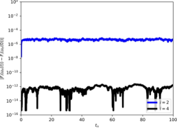
(a) Here $q=1$.

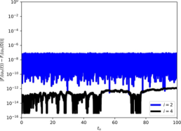
(b) Here $q=2$.

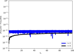
(c) Here $q=3$.

Figure 2. Here we examine the conservative discretisation scheme with various polynomial degrees, $q$, approximating the exact solution (2.21) with initial conditions given by (5.2). We show the errors measured in the $\operatorname{L}^{\infty}(0,t_{n};\operatorname{L}^{2}(\mathbb{S}^{1}))$ norm for each component of the system and the EOC for test runs that benchmark both the spatial and temporal discretisation and show that the scheme is of optimal order. We use $e_{u_{i}}:=\left\|u_{i}-U_{i}\right\|_{\operatorname{L}^{\infty}(0,t_{n};\operatorname{L}^{2}(\mathbb{S}^{1}))}$ for $i=1,2$, the components of the solution $\boldsymbol{u}=\!\left({u_{1},u_{2}}\right)^{\boldsymbol{\intercal}}$ and numerical approximation $\boldsymbol{U}=\!\left({U_{1},U_{2}}\right)^{\boldsymbol{\intercal}}$.

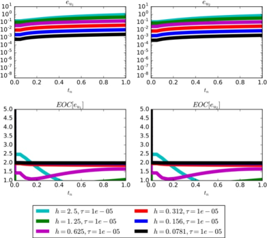
(a) Here $q=1$ and we fix $\tau{}=0.00001$. This is sufficiently small that the spatial discretisation error dominates.

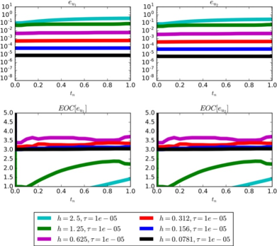
(b) Here $q=2$ and we fix $\tau=0.00001$. This is sufficiently small that the spatial discretisation error dominates.

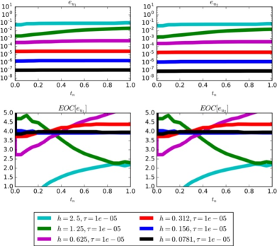
(c) Here $q=3$ and we fix $\tau=0.00001$. This is sufficiently small that the spatial discretisation error dominates.

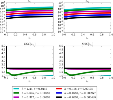
(d) Here $q=2$ and on every refinement level we choose a coupling $\tau=Ch$. Note that the time discretisation error here dominates.

5.3. Test 2 - Asymptotic benchmarking of a $2$-soliton solution

We take $d=2$ and

(5.3) $$\boldsymbol{u}_{0}=\frac{F_{\mu,\nu}}{G}\boldsymbol{E}_{1}+\frac{F_{\nu,\mu}}{G}\boldsymbol{E}_{2},$$

with $F_{\mu,\nu}$ given in (2.23) $G$ given in (2.24). The parameters are $\boldsymbol{E_{1}}=(1,0)^{\boldsymbol{\intercal}}$, $\boldsymbol{E_{2}}=(0,1)^{\boldsymbol{\intercal}}$, $\mu=\sqrt{2}$, $\nu=\sqrt{3}$, $c_{\nu}=24.9,c_{\mu}=25.1$. The exact solution is then given by (2.5). We take a uniform timestep and uniform meshes that are fixed with respect to time. Convergence results are shown in Figure 4 and conservativity over long time is given in Figure 3. Note that for $2$-soliton solution we have $\boldsymbol{W}^{n}\neq\boldsymbol{0}$ in general in which case the Lagrange multiplier is required to ensure $\int_{\mathbb{S}^{1}}\boldsymbol{V}^{n}\cdot\boldsymbol{W}^{n}=0$ for all $n$ and that the results of Theorem 4.6 hold.

Figure 3. Here we examine the conservative discretisation scheme with various polynomial degrees, $q$, approximating the exact solution (2.22) with initial conditions given by (5.3). We show the deviation in the two invariants $F_{i}$, $i=2,4$, corresponding to momentum and energy respectively. In each test we take a fixed spatial discretisation parameter of $h=0.25$ and fixed time step of $\tau=0.001$. Notice that in each case the deviation in energy is smaller than the solver tolerance of $10^{-12}$ and the deviation in momentum is bounded. The simulations are simulated for long time to test conservativity with $T=100$ in each case.

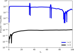
(a) Here $q=1$.

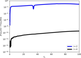
(b) Here $q=2$.

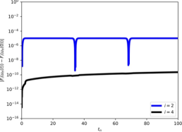
(c) Here $q=3$.

Figure 4. Here we examine the conservative discretisation scheme with various polynomial degrees, $q$, approximating the exact solution (2.22) with initial conditions given by (5.3). We show the errors measured in the $\operatorname{L}^{\infty}(0,t_{n};\operatorname{L}^{2}(\mathbb{S}^{1}))$ norm for each component of the system and the EOC for test runs that benchmark both the spatial and temporal discretisation and show that the scheme is of the correct order. We use $e_{u_{i}}:=\left\|u_{i}-U_{i}\right\|_{\operatorname{L}^{\infty}(0,t_{n};\operatorname{L}^{2}(\mathbb{S}^{1}))}$ for $i=1,2$, the components of the solution $\boldsymbol{u}=\!\left({u_{1},u_{2}}\right)^{\boldsymbol{\intercal}}$.

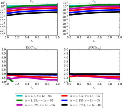
(a) Here $q=1$ and we fix $\tau{}=0.00001$. This is sufficiently small that the spatial discretisation error dominates.

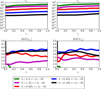
(b) Here $q=2$ and we fix $\tau{}=0.00001$. This is sufficiently small that the spatial discretisation error dominates.

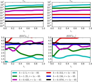
(c) Here $q=3$ and we fix $\tau{}=0.00001$. This is sufficiently small that the spatial discretisation error dominates.

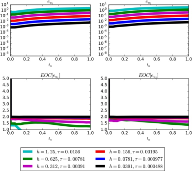
(d) Here $q=2$ and on every refinement level we choose a coupling $\tau=Ch$. Note that the time discretisation error here dominates.

5.4. Test 3 - Dynamics of $2$ and $3$-soliton solutions

Subtest 1

We take $d=2$ and

(5.4) $$\boldsymbol{u}_{0}=\frac{F_{\mu,\nu}}{G}\boldsymbol{E}_{1}+\frac{F_{\nu,\mu}}{G}\boldsymbol{E}_{2},$$

with $F_{\mu,\nu}$ given in (2.23) $G$ given in (2.24). The parameters are $\boldsymbol{E_{1}}=(\frac{9}{10},\frac{\sqrt{19}}{10})^{\boldsymbol{\intercal}}$, $\boldsymbol{E_{2}}=(\frac{1}{10},\frac{3\sqrt{11}}{10})^{\boldsymbol{\intercal}}$, $\mu=\sqrt{2}$, $\nu=\sqrt{3}$, $c_{\nu}=10,c_{\mu}=13$. Figure 5 shows some plots of the dynamics of the numerical approximation.

Subtest 2

We take $d=2$ and

(5.5) $$\boldsymbol{u}_{0}=\frac{F_{\mu,\nu}}{G}\boldsymbol{E}_{1}+\frac{F_{\nu,\mu}}{G}\boldsymbol{E}_{2},$$

with $F_{\mu,\nu}$ given in (2.23) $G$ given in (2.24). The parameters are $\boldsymbol{E_{1}}=(1,0)^{\boldsymbol{\intercal}}$, $\boldsymbol{E_{2}}=(0,1)^{\boldsymbol{\intercal}}$, $\mu=\sqrt{2}$, $\nu=\sqrt{3}$, $c_{\mu}=9,c_{\nu}=13$. Figure 6 shows some plots of the dynamics of the numerical approximation.

Subtest 3

In addition to the 2-soliton interactions we also take the opportunity to examine the dynamics of a 3-soliton interaction. We take $d=2$ and

(5.6) $$\boldsymbol{u}_{0}=\sum_{i=1}^{3}\frac{2\mu_{i}}{\cosh\!\left({\mu_{i}\!\left({x-c_{\mu_{i}}}\right)}\right)}\boldsymbol{E_{i}}$$

with $\boldsymbol{E}_{1}=\boldsymbol{E}_{3}=\!\left({1,0}\right)^{\boldsymbol{\intercal}},\boldsymbol{E}_{2}=\!\left({0,1}\right)^{\boldsymbol{\intercal}}$, $\mu_{1}=\frac{19}{10},\mu_{2}=-\frac{40}{25},\mu_{3}=\frac{13}{10}$ and $c_{\mu_{1}}=4,c_{\mu_{2}}=12,c_{\mu_{3}}=21$. Figure 7 shows the dynamics of the numerical approximation.

Figure 5. Here we show the dynamics of the approximation generated by the conservative discretisation scheme with polynomial degree $q=1$ approximating a smooth solution with initial conditions given by (5.4).

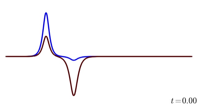
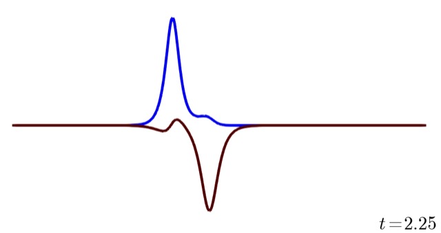
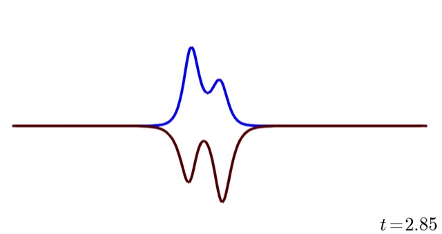
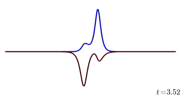
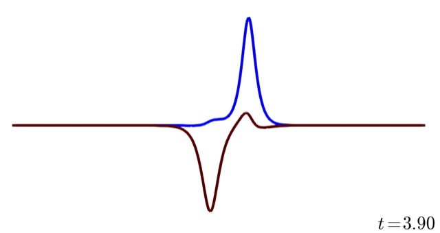
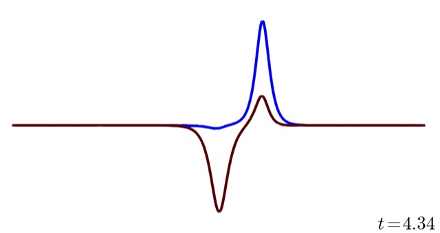
Figure 6. Here we show the dynamics of the approximation generated by the conservative discretisation scheme with polynomial degree $q=1$ approximating a smooth solution with initial conditions given by (5.5).

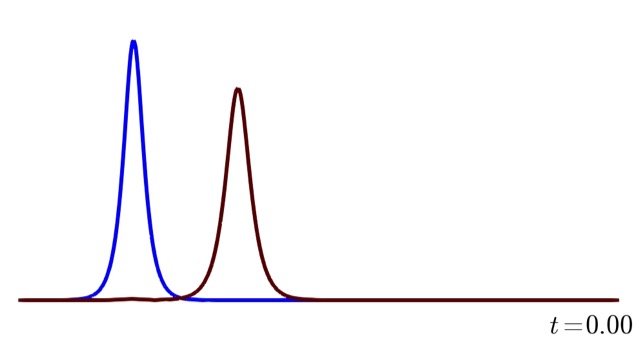
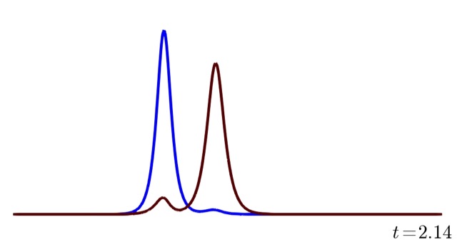
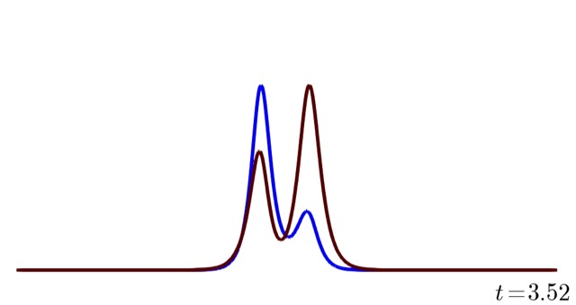
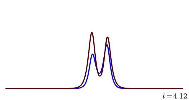
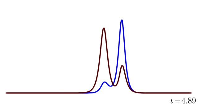
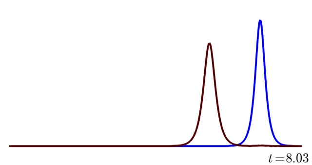
Figure 7. Here we show the dynamics of the approximation generated by the conservative discretisation scheme with polynomial degree $q=1$ approximating a smooth solution with initial conditions given by (5.6).

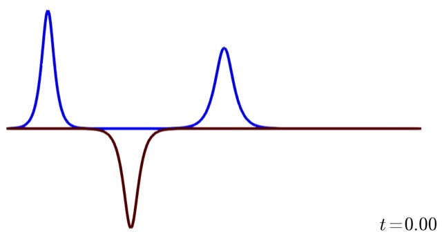
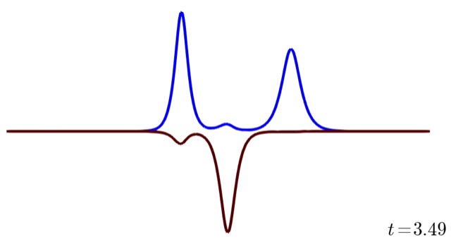
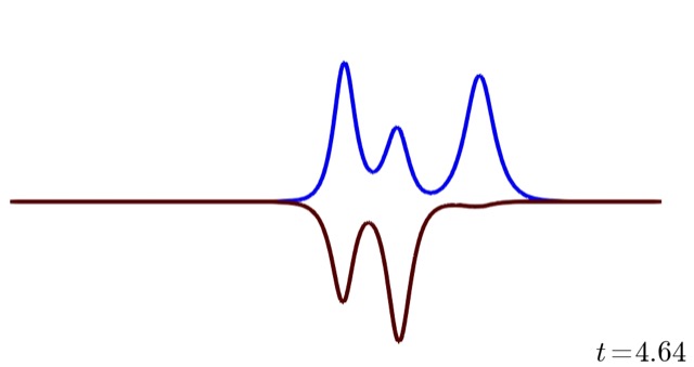
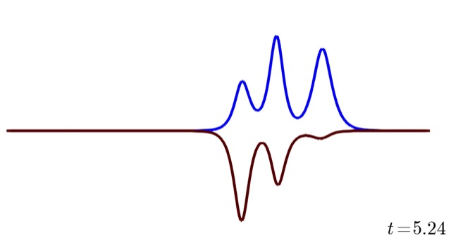
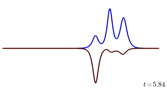
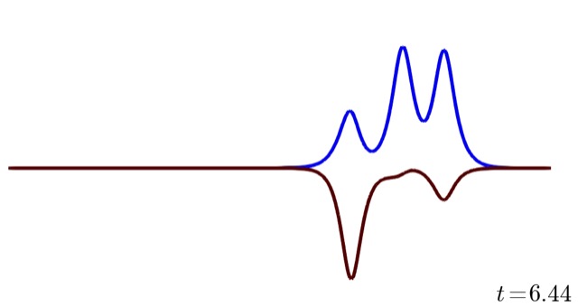
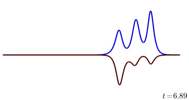
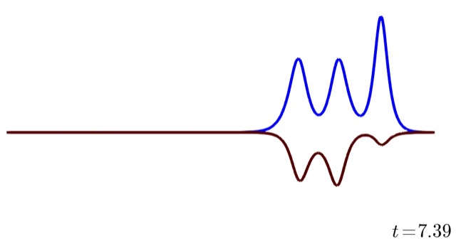
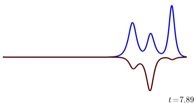
5.5. Test 4 - Propagation of solitary waves from smooth initial data

We take $d=2$ and $\boldsymbol{u}_{0}=\!\left({u_{0,1},u_{0,2}}\right)$ with

(5.7) $$\begin{split}u_{0,1}&=\operatorname{sin}\left(\frac{\pi}{20}x\right)\\ u_{0,2}&=\operatorname{cos}\left(\frac{\pi}{10}x\right).\end{split}$$

The solution here is smooth and solitary waves begin to form quickly into the simulation. Plots of the solutions are given in Figure 9 as well as conservativity plots in Figure 8.

Figure 8. Here we examine the conservative discretisation scheme with various polynomial degrees, $q$, approximating the solution to (2.2) with initial conditions given by (5.7). We show the deviation in the two invariants $F_{i}$, $i=2,4$, corresponding to momentum and energy respectively. In each test we take a fixed spatial discretisation parameter of $h=0.25$ and fixed time step of $\tau=0.001$. Notice that in each case the deviation in energy is smaller than the solver tolerance of $10^{-12}$ and the deviation in momentum is bounded. The simulations are simulated for long time to test conservativity with $T=100$ in each case.

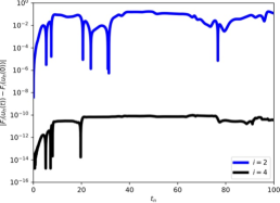
(a) $q=1$

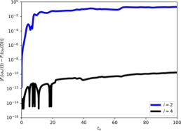
(b) $q=2$

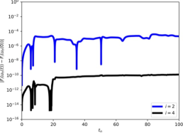
(c) $q=3$

Figure 9. Here we show the dynamics of the approximation generated by the conservative discretisation scheme with polynomial degree $q=1$ approximating the solution to (2.2) with initial conditions given by (5.8). Notice that initially, dispersive waves emanate from the discontinuity.

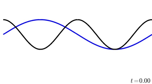
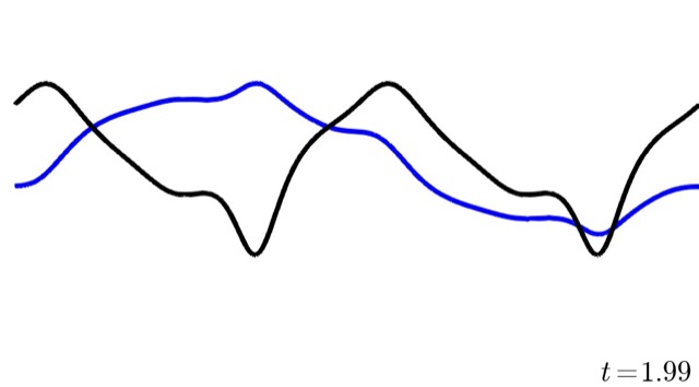
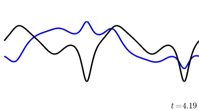
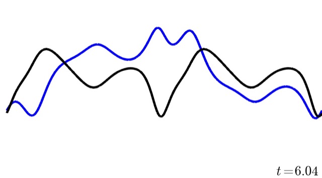
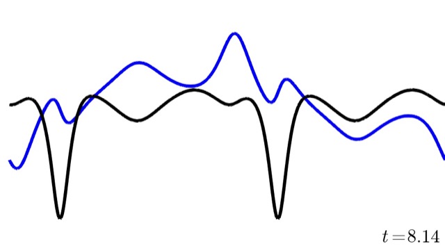
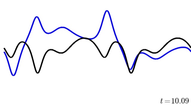
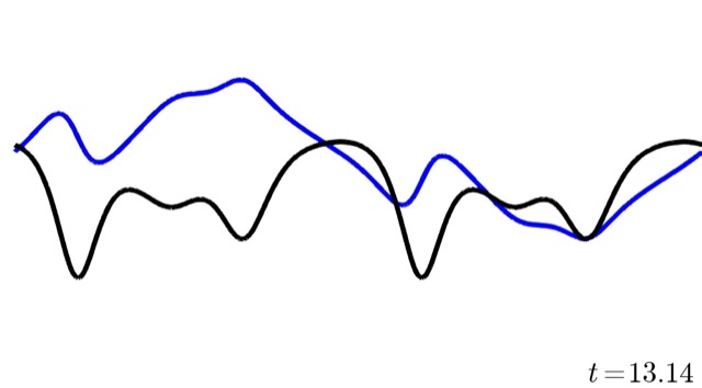
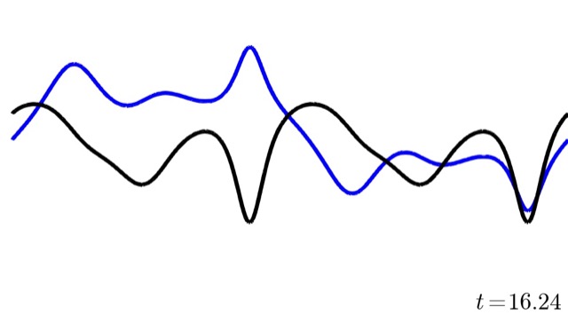
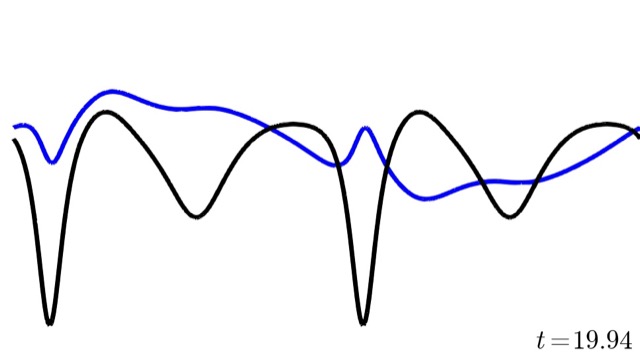
5.6. Test 5 - Solution with discontinuous initial data

We take $d=2$ and $\boldsymbol{u}_{0}=\!\left({u_{0,1},u_{0,2}}\right)$ with

(5.8) $$\begin{split}u_{0,1}&=\begin{cases}1\text{ for }x\in[10,20]\\ 0\text{ otherwise}.\end{cases}\\ u_{0,2}&=\begin{cases}0\text{ for }x\in[20,30]\\ 1\text{ otherwise}.\end{cases}\end{split}$$

The solution here is discontinuous in both components. This is a particularly tough scenario to simulate as there is no guarantee of classical solutions. We align the mesh to the discontinuities so that the discrete energy at the initial condition makes sense. Plots of the solutions are given in Figure 11 as well as conservativity plots in Figure 10.

Figure 10. Here we examine the conservative discretisation scheme with various polynomial degrees, $q$, approximating the solution to (2.2) with initial conditions given by (5.8). We show the deviation in the two invariants $F_{i}$, $i=2,4$, corresponding to momentum and energy respectively. In each test we take a fixed spatial discretisation parameter of $h=0.25$ and fixed time step of $\tau=0.001$. Notice that in each case the deviation in energy is smaller than the solver tolerance of $10^{-12}$ and the deviation in momentum is bounded. The simulations are simulated for long time to test conservativity with $T=100$ in each case.

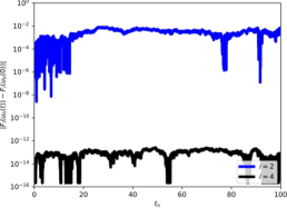
(a) $q=1$

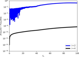
(b) $q=2$

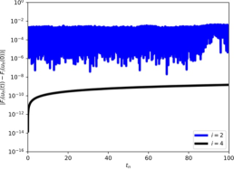
(c) $q=3$

Figure 11. Here we show the dynamics of the approximation generated by the conservative discretisation scheme with polynomial degree $q=1$ approximating the solution to (2.2) with initial conditions given by (5.8). Notice that initially, dispersive waves emanate from the discontinuity.

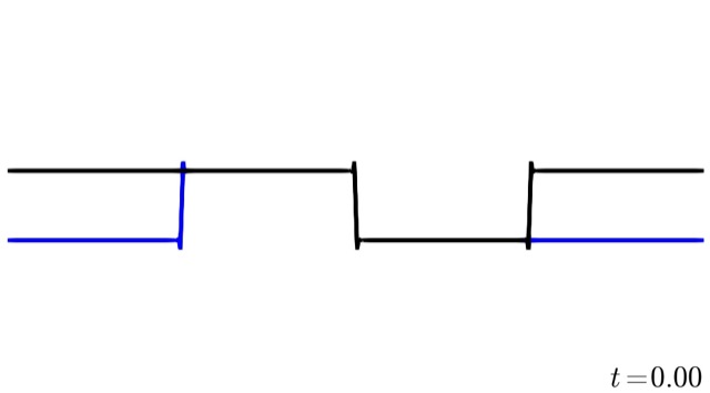
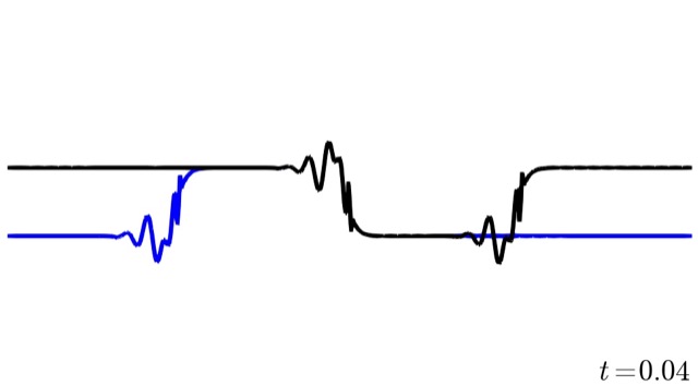
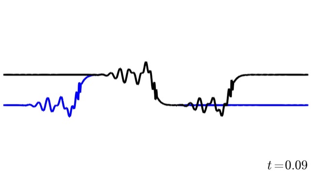
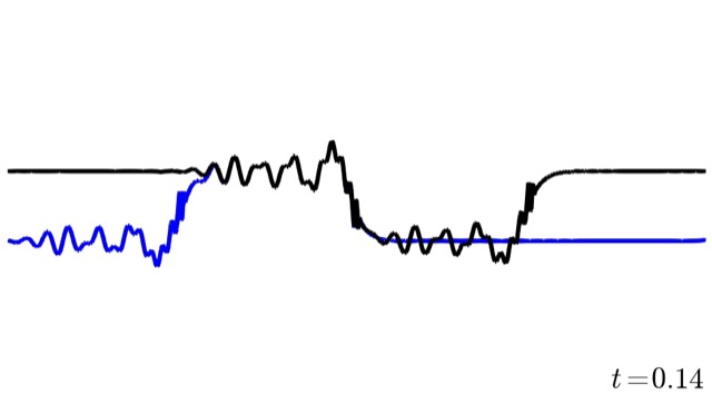
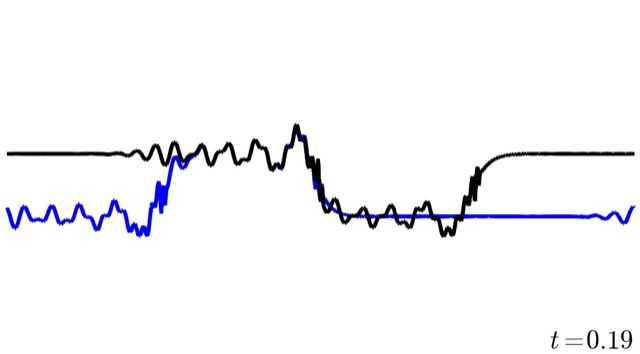
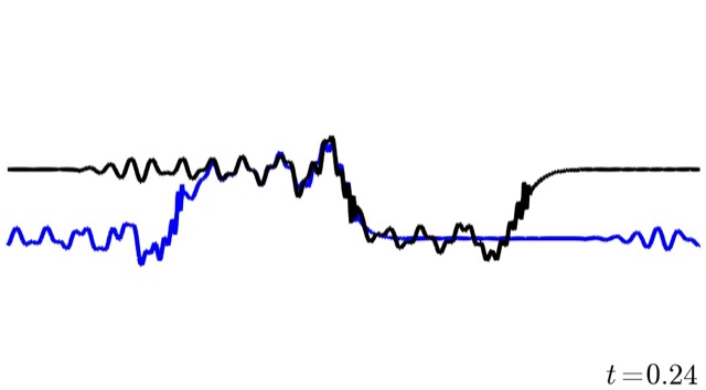
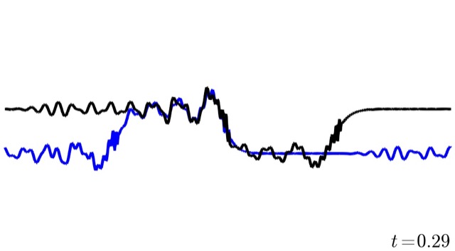
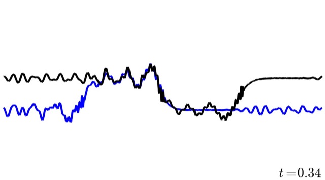
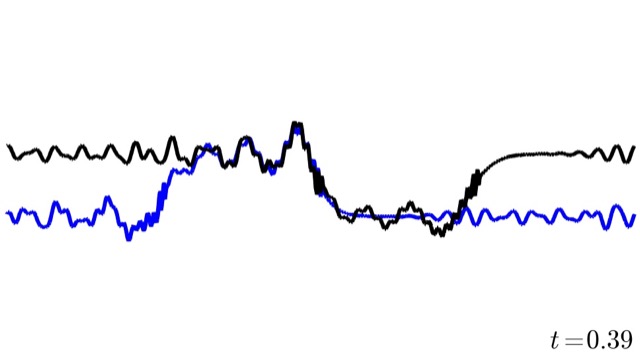
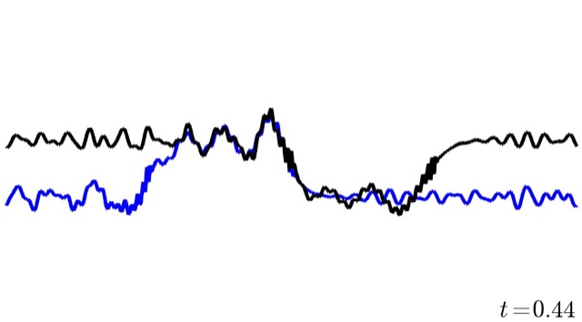
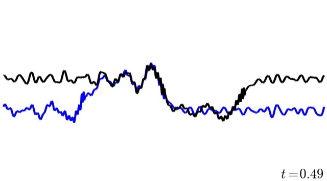
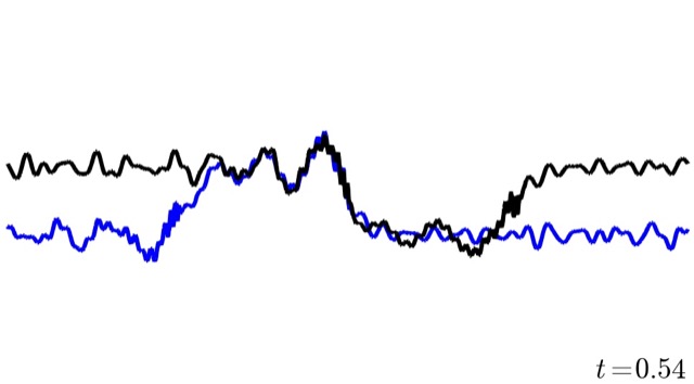
6. Conclusions

In this work we have constructed a consistent Galerkin approximation for the vmKdV equation. We have proven that both the semi-discretisations as well as the fully discrete problems are conservative and numerically shown that this is true in practice. In addition, we have given numerical evidence to suggest that the method is of optimal order, that is, $\left\|\boldsymbol{u}-\boldsymbol{U}\right\|_{\operatorname{L}^{\infty}((0,T);\operatorname{L}^{2}(\mathbb{S}^{1}))}=\operatorname{O}(\tau^{2}+h^{q+1})$. We expect methods designed in this fashion, which is quite generic, to be successful in the simulation of geophysical fluid flows.

References

- [AC91] M.J. Ablowitz and P.A. Clarkson. Solitons, nonlinear evolution equations and inverse scattering, volume 149. Cambridge university press, 1991.
- [Anc06] S.C. Anco. Hamiltonian flows of curves in g/so (n) and vector soliton equations of mkdv and sine-gordon type. SIGMA, 2, 2006.
- [ANW11] Stephen C Anco, Nestor Tchegoum Ngatat, and Mark Willoughby. Interaction properties of complex modified korteweg–de vries (mkdv) solitons. Physica D: Nonlinear Phenomena, 240(17):1378–1394, 2011.
- [AP17] P. Adamapoulou and G. Papamikos. On the hierarchy of the vector modified KdV equation. In preparation, 2017.
- [BC16] S. Blanes and F. Casas. A Concise Introduction to Geometric Numerical Integration. CRC Press, 2016.
- [BCKX13] J. L. Bona, H. Chen, O. Karakashian, and Y. Xing. Conservative, discontinuous Galerkin-methods for the generalized Korteweg-de Vries equation. Math. Comp., 82(283):1401–1432, 2013.
- [BDM07] J.L. Bona, V.A. Dougalis, and D.E. Mitsotakis. Numerical solution of KdV–KdV systems of Boussinesq equations: I. The numerical scheme and generalized solitary waves. Mathematics and Computers in Simulation, 74(2):214–228, 2007.
- [BL07] O. Bokhove and P. Lynch. Air parcels and air particles: Hamiltonian dynamics. Nieuw Arch. Wiskd. (5), 8(2):100–106, 2007.
- [BR01] T.J. Bridges and S. Reich. Multi-symplectic integrators: numerical schemes for Hamiltonian PDEs that conserve symplecticity. Phys. Lett. A, 284(4-5):184–193, 2001.
- [BZ09] D. Bai and L. Zhang. The finite element method for the coupled Schrödinger–KdV equations. Physics Letters A, 373(26):2237–2244, 2009.
- [CGM+12] E. Celledoni, V. Grimm, R. I. Mclachlan, D. I. Mclaren, D. O’Neale, B. Owren, and G. R. W. Quispel. Preserving energy resp. dissipation in numerical pdes using the ”average vector field” method. J. Comput. Phys., 231(20):6770–6789, August 2012.
- [CMR14] D. Cohen, T. Matsuo, and X. Raynaud. A multi-symplectic numerical integrator for the two-component Camassa-Holm equation. J. Nonlinear Math. Phys., 21(3):442–453, 2014.
- [COR08] D. Cohen, B. Owren, and X. Raynaud. Multi-symplectic integration of the Camassa-Holm equation. J. Comput. Phys., 227(11):5492–5512, 2008.
- [FT07] L.D. Faddeev and L. Takhtajan. Hamiltonian methods in the theory of solitons. Springer Science & Business Media, 2007.
- [Hir73] Ryogo Hirota. Exact envelope-soliton solutions of a nonlinear wave equation. Journal of Mathematical Physics, 14(7):805–809, 1973.
- [Hir04] R. Hirota. The direct method in soliton theory, volume 155. Cambridge University Press, 2004.
- [HLW06] E. Hairer, C. Lubich, and G. Wanner. Geometric numerical integration, volume 31 of Springer Series in Computational Mathematics. Springer-Verlag, Berlin, second edition, 2006. Structure-preserving algorithms for ordinary differential equations.
- [Jac17a] J. Jackaman. A conservative Galerkin method for the vectorial modified Korteweg deVries equation. In http://dx.doi.org/10.5281/zenodo.600668. 2017.
- [Jac17b] J. Jackaman. Momentum and energy conservative schemes for a class of Hamiltonian problems. In preparation, 2017.
- [JP17] J. Jackaman and T. Pryer. Conservative discontinuous Galerkin methods for Hamiltonian PDEs. In preparation, 2017.
- [KM15] O. Karakashian and Ch. Makridakis. A posteriori error estimates for discontinuous Galerkin methods for the generalized Korteweg–de Vries equation. Math. Comp., 84(293):1145–1167, 2015.
- [Lax76] P.D. Lax. Almost periodic solutions of the KdV equation. SIAM review, 18(3):351–375, 1976.
- [LR04] B. Leimkuhler and S. Reich. Simulating Hamiltonian dynamics, volume 14 of Cambridge Monographs on Applied and Computational Mathematics. Cambridge University Press, Cambridge, 2004.
- [Mag78] Franco Magri. A simple model of the integrable hamiltonian equation. Journal of Mathematical Physics, 19(5):1156–1162, 1978.
- [MBSW02] G Mari Beffa, Jan A Sanders, and Jing Ping Wang. Integrable systems in three-dimensional riemannian geometry. Journal of nonlinear science, 12(2):143–167, 2002.
- [MGO05] P. Müller, C. Garrett, and A. Osborne. Rogue waves. Oceanography, 18(3):66–75, 2005.
- [NMPZ84] S. Novikov, S.V. Manakov, L.P. Pitaevskii, and V.E. Zakharov. Theory of solitons: the inverse scattering method. Springer Science & Business Media, 1984.
- [Olv93] P.J. Olver. Applications of Lie groups to differential equations, volume 107 of Graduate Texts in Mathematics. Springer-Verlag, New York, second edition, 1993.
- [Rei00] S. Reich. Finite volume methods for multi-symplectic PDEs. BIT, 40(3):559–582, 2000.
- [RHM+16] Florian Rathgeber, David A Ham, Lawrence Mitchell, Michael Lange, Fabio Luporini, Andrew TT McRae, Gheorghe-Teodor Bercea, Graham R Markall, and Paul HJ Kelly. Firedrake: automating the finite element method by composing abstractions. ACM Transactions on Mathematical Software (TOMS), 43(3):24, 2016.
- [RN94] I. Roulstone and J. Norbury. A Hamiltonian structure with contact geometry for the semi-geostrophic equations. J. Fluid Mech., 272:211–233, 1994.
- [RS02] C. Rogers and W.K. Schief. Bäcklund and Darboux transformations: geometry and modern applications in soliton theory, volume 30. Cambridge University Press, 2002.
- [She90] T.G. Shepherd. Symmetries, Conservation Laws, and Hamiltonian Structure in Geophysical Fluid Dynamics. Advances in Geophysics, 32:287 – 338, 1990.
- [SM91] M.A. Salle and V.B. Matveev. Darboux transformations and solitons., 1991.
- [SW03] Jan A Sanders and Jing Ping Wang. Integrable systems in n-dimensional riemannian geometry. Moscow Mathematical Journal, 3(4):1369–1393, 2003.
- [Win80] R. Winther. A conservative finite element method for the Korteweg-de Vries equation. Math. Comp., 34(149):23–43, 1980.
- [XS07] Y. Xu and C.W. Shu. Error estimates of the semi-discrete local discontinuous Galerkin method for nonlinear convection-diffusion and KdV equations. Comput. Methods Appl. Mech. Engrg., 196(37-40):3805–3822, 2007.
- [YS02] J. Yan and C.W. Shu. A local discontinuous Galerkin method for KdV type equations. SIAM J. Numer. Anal., 40(2):769–791 (electronic), 2002.