Yet another skew-elliptical family but of a different kind: return to Lemma 1

Abstract

In the context of modulated-symmetry distributions, there exist various forms of skew-elliptical families. We present yet another one, but with an unusual feature: the modulation factor of the baseline elliptical density is represented by a distribution function with an argument which is not an odd function, as it occurs instead with the overwhelming majority of similar formulations, not only with other skew-elliptical families. The proposal is obtained by going back to the use of Lemma 1 of Azzalini and Capitanio (1999), which can be seen as the general frame for a vast number of existing formulations, and use it on a different route. The broader target is to show that this ‘mother lemma’ can still generate novel progeny.

Some key-words: elliptical distributions, skew-elliptical distributions, symmetry-modulated distributions.

1 Background and aims

In the last fifteen years or so, there has been a formidable development on the theme of ‘symmetry-modulated distributions’, also called ‘skew-symmetric distributions’. In the context of continuous random variables, the key tool for building a symmetry-modulated distribution starting from a centrally symmetric density $f_{0}$ on $\mathbb{R}^{d}$, that is, such that $f_{0}(x)=f_{0}(-x)$, is represented by the expression

$$f(x)=2\>f_{0}(x)\>G_{0}\{w(x)\}\,,\qquad\quad x\in\mathbb{R}^{d},$$ (1)

where $G_{0}$ is a univariate continuous distribution function such that $G_{0}(-x)=1-G_{0}(x)$, that is, it establishes to a symmetric distribution about $0$, and $w(\cdot)$ is a real-valued function such that $w(-x)=-w(x)$. Under the stated conditions, for any ‘baseline’ density $f_{0}$ and any choice of the ingredients $G_{0}$ and $w$ which enter the final ‘modulating term’ of $f(x)$, this is a proper density.

The above passage has reproduced Proposition 1 of Azzalini & Capitanio (2003). A slightly different formulation, essentially equivalent to the one above, has been presented by Wang et alii (2004). Even a brief summary of the developments stemming from the symmetry-modulated distributions in 1 would take an enormous space. For such objective, the reader is referred to the recent account by Azzalini & Capitanio (2014). Here we limit ourselves to recall the facts directly related to our plan of work.

The fact that 1 constitutes a density function is actually a corollary of a more general result, namely Lemma 1 of Azzalini & Capitanio (1999); its exact statement will be recalled in the next section. Right after this lemma, Azzalini and Capitanio formulated an immediate corollary by taking $f_{0}$ of elliptical type and $w$ of linear type. That corollary prompted a stream of literature focusing on successive layers of generalizations, where $f_{0}$ fulfils some symmetry condition and $w$ is odd, eventually leading to symmetry-modulated distributions.

There exist, however, other constructions encompassed by the above-quoted Lemma 1, falling outside the domain of symmetry-modulated distributions in 1. This territory has been barely explored. As far as we known, the only two publications of this sort are those of Azzalini (2012) and Jupp et alii (2016). The broad target of the present note is to investigate further this area. In spite of the common domain of interest, operationally there is little overlap between our development and the publications just quoted.

The present specific contribution, developed along the indicated direction, is constituted by a new proposal of skew-elliptical or, equivalently, skew-elliptically contoured (SEC) density. A number of SEC constructions in the form of symmetry modulated densities, obtained by some form of perturbation of an elliptically contoured (EC) density, have already been examined in the literature. Besides the above-mentioned ‘linear-type’ SEC, the more commonly adopted form of SEC is the one introduced by Branco & Dey (2001) via a selection mechanism applied to an elliptical distribution. In their exposition, it was not evident that their SEC distribution had a structure like 1, but this was shown in some important special cases by Azzalini & Capitanio (2003) and later in general by Azzalini & Regoli (2012, p. 872). An additional form of SEC distribution has been presented by Sahu et alii (2003).

There is structural difference between the existing SEC distributions and the one to be presented here. Because of its genesis, the new SEC is not constrained by the conditions pertaining to 1. It obviously retains the fact that $f_{0}$ is of elliptical class, otherwise the term SEC would not apply to it, but its $w(\cdot)$ does not satisfy the condition $w(-x)=-w(x)$.

2 A ‘mother’ lemma

The wording of the next statement is slightly different from the one in the original source, but completely equivalent to it. The expression ‘symmetric about $0$’ is an abbreviated term for ‘symmetrically distributed about $0$’, in case of a univariate random variable. We also use the term ‘symmetric about $0$’ for a univariate distribution function $H$ such that $H(-x)=1-H(x)$.

Lemma 1 (Azzalini & Capitanio, 1999)

Denote by $G_{0}$ the continuous distribution function of a univariate random variable symmetric about $0$, by $w(\cdot)$ a real-valued function on $\mathbb{R}^{d}$ and by $Z_{0}$ a $d$-dimensional variable with density function $f_{0}$, such that $W=w(Z_{0})$ is symmetric about $0$. Then

$$f(x)=2\>f_{0}(x)\>G_{0}\{w(x)\}\,,\qquad x\in\mathbb{R}^{d},$$ (2)

is a density function.

At first sight, the distribution in 2 coincides with 1. While the mathematical expressions look the same, the meaning of their symbols, and consequently their mathematical meaning, are largely different:

• in 2, $f_{0}$ is not required to satisfy the condition $f_{0}(-x)=f_{0}(x)$;

• in 2, $w$ is not required to satisfy the condition $w(-x)=-w(x)$;

• the only common assumption is that $G_{0}(-x)=1-G_{0}(x)$.

The key point for applying Lemma 1 is that $W=w(Z_{0})$ is symmetric about 0. Once this holds, any $G_{0}$ symmetric about 0 can be adopted to build a valid density. This scheme was particularly simple in the first application of the lemma, namely Corollary 2 of Azzalini & Capitanio (1999): if $Z_{0}$ is elliptical centred at 0, then the linear transform $w(Z_{0})=a^{\top}\,Z_{0}$ is symmetric about 0 for any choice of the vector $a$ of coefficients and this suffices for applying the lemma, irrespective of the choice of $G_{0}$. It only takes a little more effort along the same line of argument to show that $f(x)$ in 1 is a proper density.

We also recall the stochastic representation for distribution 2 stated by Azzalini & Capitanio (1999, p. 599). If $X$ is a $d$-dimensional variable with density $f_{0}$ and $T$ is an independent variable with distribution function $G_{0}$, satisfying the conditions of Lemma 1, then

$$Z=\cases{X&if $T\leq w(X)$\cr-X&otherwise}$$ (3)

has distribution 2.

Besides symmetry-modulated distributions, Lemma 1 embraces other constructions, although so far these have little been studied, as already mentioned. This overarching capability of Lemma 1 explains the term ‘mother lemma’ which we have employed. The aim of the present note is to examine a case of this sort, specifically when $f_{0}$ is an elliptical density.

3 Functions of orthogonal elliptical components

We want to examine a construction where the density function $f_{0}$ of $Z_{0}$ is of EC type and $W=w(Z_{0})$ is symmetric about 0.

Start by considering the case where $f_{0}$ is a bivariate elliptically contoured distribution with ‘standardized’ marginals. Specifically, assume that $f_{0}$ is the density function of

$$\pmatrix{X\cr Y}\sim\mathrm{EC}_{2}\left(\matrix{0\cr 0},\pmatrix{1&\rho\cr\rho&1},\psi\right)$$ (4)

following the notation adopted by Fang et alii (1990), up to a minor change in the symbol of the ‘generator’, $\psi$ for us.

Proposition 2

Given the continuous random variable $(X,Y)$ with distribution as in 4, the transformed variable

$$W=(Y-\rho X)\>h(X)$$ (5)

has is symmetric about 0 for any choice of the real-valued function $h$.

Proof From Theorem 2.18 of Fang et alii (2012), the conditional distribution of $W$ given $X=x$ is

$$(W|X=x)\sim\mathrm{EC}_{1}(0,(1-\rho^{2})\,h(x)^{2},\psi_{x})$$

where $\psi_{x}$ is another generator, which in general depends on $x$, but its explicit expression is irrelevant to us. All we need is that the corresponding density $f_{W|x}(w)$ is symmetric about 0, so that $f_{W|x}(w)=f_{W|x}(-w)$. Therefore the unconditional density of $W$ is

$$f_{W}(w) = \int_{\mathbb{R}}f_{W|x}(w)\>f_{0X}(x)\,\mathrm{d}{x}$$

$$= \int_{\mathbb{R}}f_{W|x}(-w)\>f_{0X}(x)\,\mathrm{d}{x}$$

$$= f_{W}(-w)\,.$$

by integration with respect to the distribution $f_{0X}(x)$ of the $X$ component. qed

This result can immediately be extended to a general $d$-dimensional continuous random variable with EC distribution $(d>1)$, whose components are partitioned as follows:

$$\pmatrix{X\cr Y}\sim\mathrm{EC}_{d}\left(\mu,\Sigma,\psi\right),\qquad\mu=\pmatrix{\mu_{x}\cr\mu_{y}},\quad\Sigma=\pmatrix{\Sigma_{11}&\sigma_{12}\cr\sigma_{21}&\sigma_{22}}$$ (6)

where now $X$ is $(d-1)$-dimensional; $W$ takes now the more general form

$$W=\big{(}Y-m_{Y}(X)\big{)}\>h(X)\,\quad\mathrm{or}\quad W=\frac{Y-m_{Y}(X)}{(\sigma_{22\cdot 1})^{1/2}}\>h(X)$$ (7)

where

$$m_{Y}(X) = \mu_{y}+\sigma_{21}\Sigma_{11}^{-1}(X-\mu_{x})=\beta_{0}+\beta^{\top}X\,,\leavevmode\nobreak\ \mathrm{say},$$ (8)

$$\sigma_{22\cdot 1} = \sigma_{22}-\sigma_{21}\Sigma_{11}^{-1}\sigma_{12}$$ (9)

are as in equation (2.42) of Fang et alii (2012). In case the mean value of $Y$ conditionally on $X$, it coincides with 8. The second form of 7 is just a minor variant of the first one, but it is conceptually convenient to have the first factor ‘standardized’, in the sense of being free from scale factors, besides the location parameter. Finally, note that symmetry about 0 persists if $Y-m_{Y}(X)$ is transformed to $w_{0}(Y-m_{Y}(X))$ by an odd function $w_{0}$.

We can summarize the combination of the above discussion and Lemma 1 into the following conclusion.

Proposition 3

Denote by $f_{0}(x,y)$ the $d$-dimensional elliptically contoured density of the random variable $(X,Y)$ in 6, by $G_{0}$ a continuous distribution function such that $G_{0}(-x)=1-G_{0}(x)$ and by $w(x,y)$ either of the two forms

$$w(x,y)=w_{0}\big{(}y-m_{Y}(x)\big{)}\>h(x)\,,\quad\quad w(x,y)=w_{0}\left(\frac{y-m_{Y}(x)}{(\sigma_{22\cdot 1})^{1/2}}\right)\>h(x)$$ (10)

for any function $h(x)$ from $\mathbb{R}^{d-1}$ to $\mathbb{R}$ and any odd function $w_{0}$ on the real line; here $m_{Y}(\cdot)$ and $\sigma_{22\cdot 1}$ are given by 8 and 9. Then

$$f(x,y)=2\>f_{0}(x,y)\>G_{0}\{w(x,y)\}$$ (11)

is a proper density function.

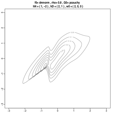
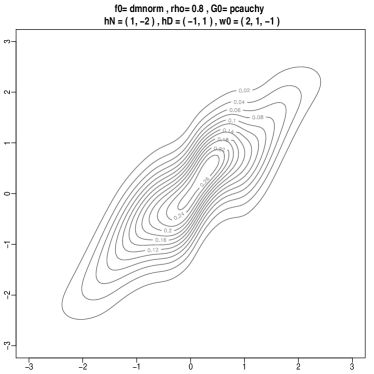
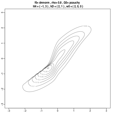
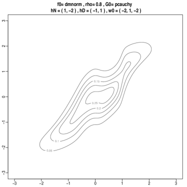
Some example bivariate densities $f(x,y)$ of the type introduced in Proposition 3 are displayed in Figure 1 in the form of contour level plots. The second form of 10 has been used and the other ingredients are as follows: $f_{0}(x)=\varphi_{2}(x;\Sigma)$ where $\Sigma$ is the same matrix occurring in 4, $G_{0}$ is the standard Cauchy distribution function and

$$h(x)=\frac{h_{N}(x)}{h_{D}(x)}=\frac{1+a_{1}\,x+a_{2}\,x^{2}}{1+b_{1}\,x+b_{2}\,x^{2}}\,,\hskip 40.00006ptw_{0}(x)=\frac{c_{1}\,x+c_{3}\,x^{3}}{1+c_{2}\,x^{2}}$$ (12)

for various choices of the coefficients $a,b,c$ and the correlation $\rho$ in $\Sigma$. The specific choices of the coefficients $a,b,c$ are indicated at the top of each pane of Figure 1. The plots indicate a wide flexibility of the family of distribution, even employing a relatively limited number of cofficients in the ratios 12.

Figure 1: Example plots of densities defined in Proposition 3 using functions in 12.

The general stochastic representation 3 applies directly to distribution 11.

4 The unperturbed component

Consider the $d$-dimensional density

$$f(x,y)=2\>f_{0}(x,y)\>G_{0}\{(y-\beta_{0}-\beta^{\top}x)\>h(x)\},\qquad\qquad x\in\mathbb{R}^{d-1},\quad y\in\mathbb{R},$$ (13)

where $f_{0}$ is as in 6 and we use the expression in 8. If $(\tilde{X},\tilde{Y})$ is a random variable with density 13, the marginal distribution of $\tilde{X}$ is

$$f_{\tilde{X}}(x) = \int_{\mathbb{R}}f(x,y)\,\mathrm{d}{y}$$

$$= \int_{\mathbb{R}}2\>f_{0,X}(x)\>f_{0,Y|x}(y)\>G_{0}\{(y-\beta_{0}-\beta^{\top}x)\>h(x)\}\,\mathrm{d}{y}$$

$$= f_{0,X}(x)\int_{\mathbb{R}}2\>f_{0,Y|x}(z)\>G_{0}(z\>\sigma_{22\cdot 1}\>h(x))\,\mathrm{d}{z}$$

$$= f_{0,X}(x)$$

on recalling (i) the expressions of the conditional mean 8 and the scale factor 9, (ii) the fact that $f_{0,Y|x}(\cdot)$ is symmetric about its mean (conditional) value, (iii) Lemma 1 of Azzalini (1985).

Therefore the marginal distribution $f_{\tilde{X}}$ of the first ${d{-}1}$ component variables after the perturbation operation is equal to the original unperturbed density $f_{0,X}$.

5 Moment generating function in a simple case

We want to compute the moment generating function (MGF) for the basic case 4 of normal type, $W$ as in 5 and $G_{0}=\Phi$. In other words, consider the density

$$f(x,y)=2\varphi(x,y;\rho)\Phi\{(y-\rho x)\>h(x)\}\,,\qquad(x,y)\in\mathbb{R}^{2}.$$ (14)

For notational convenience, we modify slightly the notation and, from now on, we use $(X,Y)$ to denote a random variable with distribution 14. The MGF of $(X,Y)$ is

$$M(t_{1},t_{2}) = \int_{\mathbb{R}}\int_{\mathbb{R}}\exp(t_{1}x+t_{2}y)\>f(x,y)\,\mathrm{d}{x}\,\mathrm{d}{y}$$

$$= 2\int_{\mathbb{R}}e^{t_{1}x}M_{c}(t_{2},x)\varphi(x)\,\mathrm{d}{x}$$

where

$$M_{c}(t_{2},x) = \int_{\mathbb{R}}e^{t_{2}y}\>f_{0,Y|x}(y)\>\Phi\{(y-\rho x)\>h(x)\}\,\mathrm{d}{y}$$

$$= \int_{\mathbb{R}}e^{t_{2}y}\varphi\left(\frac{y-\rho x}{\sqrt{1-\rho^{2}}}\right)\frac{1}{\sqrt{1-\rho^{2}}}\>\Phi\{(y-\rho x)\>h(x)\}\,\mathrm{d}{y}$$

$$= \exp(t_{2}\rho x)\int_{\mathbb{R}}\exp\left(t_{2}z\sqrt{1-\rho^{2}}\right)\>\varphi(z)\>\>\Phi\left(z\sqrt{1-\rho^{2}}\>h(x)\right)\,\mathrm{d}{z}$$

$$= \exp(t_{2}\rho x)\int_{\mathbb{R}}\frac{1}{\sqrt{2\pi}}\>\exp\left\{-\mbox{$\textstyle\frac{1}{2}$}\left[z^{2}-2\,t_{2}z\sqrt{1-\rho^{2}}\pm t_{2}^{2}(1-\rho^{2})\right]\right\}\>\Phi\left(z\sqrt{1-\rho^{2}}\>h(x)\right)\,\mathrm{d}{z}$$

$$= \exp\left[t_{2}\rho x+\mbox{$\textstyle\frac{1}{2}$}t_{2}^{2}(1-\rho^{2})\right]\int_{\mathbb{R}}\varphi(u)\,\Phi\left\{\left(u+t_{2}\sqrt{1-\rho^{2}}\right)\>h(x)\right\}\,\mathrm{d}{u}$$

$$= \exp\left[t_{2}\rho x+\mbox{$\textstyle\frac{1}{2}$}t_{2}^{2}(1-\rho^{2})\right]\>\Phi\left(\frac{t_{2}\,(1-\rho^{2})\,h(x)}{\sqrt{1+(1-\rho^{2})\,h(x)^{2}}}\right)$$

where the last equality follows from Corollary 1 of Ellison’s (1964) Theorem 2. Therefore

$$M(t_{1},t_{2})=2\>\exp\left\{\mbox{$\textstyle\frac{1}{2}$}t_{2}^{2}(1-\rho^{2})\right\}\>\int_{\mathbb{R}}\exp\{x(t_{1}+t_{2}\rho)\}\>\Phi\left(\frac{t_{2}\,(1-\rho^{2})\,h(x)}{\sqrt{1+(1-\rho^{2})\,h(x)^{2}}}\right)\varphi(x)\,\mathrm{d}{x}\,.$$

The above integral does not lend itself to explicit solution. To compute the moment of the $X$ and $Y$ components of 14, we exchange the integration and differentiation steps; hence consider

$$\left.\displaystyle\frac{\partial M}{\partial t_{1}}\right|_{t_{1}=t_{2}=0}\quad\mathrm{and}\quad\left.\displaystyle\frac{\partial M}{\partial t_{2}}\right|_{t_{1}=t_{2}=0}$$

with differentiation under the integration sign. The first expression leads to $\mathbb{E}\!\left\{\displaystyle{X}\right\}=0$, as expected, since the marginal density of $X$ is $\varphi(x)$, from § 4. The second expression leads to

$$\mathbb{E}\!\left\{\displaystyle{Y}\right\}=\sqrt{\frac{2}{\pi}}\>(1-\rho^{2})\>\int_{\mathbb{R}}\frac{h(x)}{\sqrt{1+(1-\rho^{2})\,h(x)^{2}}}\>\varphi(x)\,\mathrm{d}{x}\,.$$ (15)

A very special case

As a simple check of the above result, consider the elementary case $h(x)\equiv 1$, for which 15 lends

$$\sqrt{\frac{2}{\pi}}\>\frac{(1-\rho^{2})}{\sqrt{2-\rho^{2}}}\,.$$

In this case, 14 is of type

$$\mathrm{SN}{}_{2}\left(\xi=\pmatrix{0\cr 0},\Omega=\pmatrix{1&\rho\cr\rho&1},\alpha=\pmatrix{-\rho\cr 1}\right)$$

and known formulae such as (5.31) and (5.11) of the Azzalini & Capitanio (2014) say that

$$\mathbb{E}\!\left\{\displaystyle{\pmatrix{X\cr Y}}\right\}=\sqrt{\frac{2}{\pi}}\>\pmatrix{0\cr\displaystyle{\frac{1-\rho^{2}}{\sqrt{2-\rho^{2}}}}}.$$

Addition numerical checks with other choices of $h$ confirm expression 15 by use of numerical integration.

Other feasible solutions

The explicit expression of the integral in 15 is feasible only in favourable cases.

A relatively common situation occurs when $h(x)$ is odd, so that the integrand of 15 is odd and

$$\mathbb{E}\!\left\{\displaystyle{Y}\right\}=0\,.$$

Note that, when $h$ is odd, $w(x,y)=(y-\rho x)\>h(x)$ is an even function of $(x,y)$. The special case $h(x)=\alpha x$ reduces to the distribution in the first expression of equation (17) of Azzalini (2012).

Another class of functions for which explicit integration is feasible is as follows. Suppose $s(x)$ is a function for which $\mathbb{E}\!\left\{\displaystyle{s(Z)}\right\}$ is known to be $S$, say, when $Z\sim\mathrm{N}{}(0,1)$. Then solve

$$\frac{h(x)}{\sqrt{1+(1-\rho^{2})\>h(x)^{2}}}=s(x)$$

and obtain

$$h(x)=\frac{s(x)}{\sqrt{1-(1-\rho^{2})\>s(x)^{2}}}\,.$$

For this choice of $h(x)$, we can say that, by construction,

$$\mathbb{E}\!\left\{\displaystyle{Y}\right\}=\sqrt{\frac{2}{\pi}}\>(1-\rho^{2})\>S\,.$$

An especially simple example is $s(x)=\cos x$, such that $S=e^{-1/2}$, leading to

$$h(x)=\frac{\cos x}{\sqrt{1-(1-\rho^{2})\>(\cos x)^{2}}}\,,\qquad\mathbb{E}\!\left\{\displaystyle{Y}\right\}=\sqrt{\frac{2}{\pi\>e}}\>(1-\rho^{2})\,.$$

Another special case leading to a solution, with help from the Maxima symbolic manipulation system, is $h(x)=\alpha|x|$ for which we obtain

$$\mathbb{E}\!\left\{\displaystyle{Y}\right\}=\frac{2}{\sqrt{1-\rho^{2}}}\>\left[1-\Phi\left(\frac{1}{\alpha\sqrt{1-\rho^{2}}}\right)\right]\exp\left(\frac{1}{2\>\alpha^{2}(1-\rho^{2})}\right)\,.$$

Although in many other cases 15 does not lend itself to an explicit expression, it still simplifies computation with respect to direct two-dimensional numerical integration of $y\,f(x,y)$, since 15 requires only one-dimensional integration.

6 Extension to multivariate $Y$

Consider the more general case where $Y$ is $m$-dimensional, with $1\leq m<d$. Hence write the joint distribution of $(X,Y)$ as

$$\pmatrix{X\cr Y}\sim\mathrm{EC}_{d}\left(\mu,\Sigma,\psi\right),\qquad\mu=\pmatrix{\mu_{x}\cr\mu_{y}},\quad\Sigma=\pmatrix{\Sigma_{11}&\Sigma_{12}\cr\Sigma_{21}&\Sigma_{22}}$$ (16)

where $X$ is $(d-m)$-dimensional. We want to extend the expressions in 5 and 7 to this new case.

Proposition 4

For a $d$-dimensional variable $(X,Y)$ distributed as in 16, consider the transform

$$W=w_{0}\left(Y-m_{Y}(X)\right)\>h(X)$$ (17)

where $h$ is an arbitrary function function and $w_{0}$ is an odd function, that is, $w_{0}(u)\in\mathbb{R}$ and $w_{0}(-u)=-w_{0}(u)$ for $u\in\mathbb{R}^{m}$. Then $W$ is distributed symmetrically around 0.

Proof. Write $U=Y-m_{Y}(X)$ and $W_{0}=w_{0}(U)$. First we show that the distribution of $W_{0}$ conditionally on $X=x$ is symmetric about 0, for any given $x$; in fact

$$\mathbb{P}\!\left\{\displaystyle{W_{0}\leq t|X=x}\right\} = \mathbb{P}\!\left\{\displaystyle{-W_{0}\geq-t|X=x}\right\}$$

$$= \mathbb{P}\!\left\{\displaystyle{w_{0}(-U)\geq-t|X=x}\right\}$$

$$= \mathbb{P}\!\left\{\displaystyle{w_{0}(U)\geq-t|X=x}\right\}$$

$$= \mathbb{P}\!\left\{\displaystyle{W_{0}\geq-t|X=x}\right\}$$

for any real $t$, and the last equality implies symmetry of $(W_{0}|X=x)$. Then argue like in Proposition 2 to conclude that $W$ is symmetric about 0. qed

Corollary 5

Under the assumption of Proposition 3, denote by $f_{0}$ the density of 16 and let $\beta_{0}+\beta^{\top}x=m_{Y}(x)$ as given in equation (2.42) of Fang et alii (2012). Then expression 11 with

$$w(x,y)=w_{0}(y-\beta_{0}-\beta^{\top}x)\>h(x)$$

is a proper density function.

References

Azzalini, A. (1985). A class of distributions which includes the normal ones. Scand. J. Statist., 12, 171–178.

Azzalini, A. (2012). Selection models under generalized symmetry settings. Annals of the Institute of Statistical Mathematics, 64, 737–750.

Azzalini, A., and Capitanio, A. (1999). Statistical applications of the multivariate skew normal distribution. J. R. Statist. Soc., ser. B, 61, 579–602. Full version of the paper at arXiv.org:0911.2093.

Azzalini, A., and Capitanio, A. (2003). Distributions generated by perturbation of symmetry with emphasis on a multivariate skew $t$ distribution. J. R. Statist. Soc., ser. B, 65, 367–389. Full version of the paper at arXiv.org:0911.2342.

A. Azzalini, with the collaboration of A. Capitanio (2014). The Skew-Normal and Related Families. Cambridge University Press, Cambridge.

Azzalini, A., and Regoli, G. (2012). Some properties of skew-symmetric distributions. Ann. Inst. Statist. Math., 64, 857–879. Available online 09 Sept 2011.

Ellison, B. E. (1964). Two theorems for inferences about the normal distribution with applications in acceptance sampling. J. Amer. Statist. Assoc., 59, 89–95.

Fang, K.-T., Kotz, S., and Ng, K. W. (1990). Symmetric multivariate and related distributions. London: Chapman & Hall.

Jupp, P. E., Regoli, G. and Azzalini, A. (2016) A general setting for symmetric distributions and their relationship to general distributions. Journal of Multivariate Analysis 148, 107-–119.

Sahu, K., Dey, D. K., and Branco, M. D. 2003. A new class of multivariate skew distributions with applications to Bayesian regression models. Canad. J. Statist., 31, 129–150. Corrigendum: vol. 37 (2009) , 301–302.

Wang, J., Boyer, J., and Genton, M. G. (2004). A skew-symmetric representation of multivariate distributions. Statist. Sinica, 14, 1259–1270.