Thermodynamic properties of the Dynes superconductors

Abstract

The tunneling density of states in dirty superconductors is often well described by the phenomenological Dynes formula. Recently we have shown that this formula can be derived, within the coherent potential approximation, for superconductors with simultaneously present pair-conserving and pair-breaking impurity scattering. Here we demonstrate that the theory of such so-called Dynes superconductors is thermodynamically consistent. We calculate the specific heat and critical field of the Dynes superconductors, and we show that their gap parameter, specific heat, critical field, and penetration depth exhibit power-law scaling with temperature in the low-temperature limit. We also show that, in the vicinity of a coupling constant-controlled superconductor to normal metal transition, the Homes law is replaced by a different, pair-breaking dominated scaling law.

I Introduction

It is well known that, in the limit of low temperatures, the tunneling density of states of dirty superconductors $N(\omega)$ is often well described by the phenomenological Dynes formula:Dynes78 ; Noat13 ; Szabo16

$$N(\omega)=N_{0}{\rm Re}\left[\frac{\omega+i\Gamma}{\sqrt{(\omega+i\Gamma)^{2}-{\Delta}^{2}}}\right],$$ (1)

where $N_{0}$ is the normal-state density of states, $\Delta$ is the superconducting order parameter, and $\Gamma$ measures the number of in-gap states. The square root in Eq. (1) has to be taken so that its imaginary part is positive and we keep this convention throughout this paper.

Recently we have shown,Herman16 within the coherent potential approximation (CPA), that Eq. (1) applies to superconductors in which, in addition to the usual pair-conserving disorder, additional classical pair-breaking disorder field is also present. The crucial assumption which we had to make was that the pair-breaking potentials were described by a Lorentzian distribution with width $\Gamma$. The resulting $2\times 2$ Nambu-Gor’kov electron Green’s function is described by three energy scales: the order parameter $\Delta$, the pair-conserving scattering rate $\Gamma_{s}$, and the pair-breaking scattering rate $\Gamma$:Herman17

$$\hat{G}({\bf k},\omega)=\frac{1}{2}\not{\partial}\ln\left[\varepsilon_{\bf k}^{2}-\epsilon(\omega)^{2}\right],$$ (2)

where $\not{\partial}=\tau_{0}\frac{\partial}{\partial\omega}-\tau_{1}\frac{\partial}{\partial\Delta}-\tau_{3}\frac{\partial}{\partial\varepsilon_{\bf k}}$ resembles the Feynman slash derivative, $\tau_{i}$ are the Pauli matrices, and

$$\epsilon(\omega)=\sqrt{(\omega+i\Gamma)^{2}-\Delta^{2}}+i\Gamma_{s}.$$ (3)

In Ref. Herman17, we have argued that Eqs. (2,3) represent the simplest internally consistent extension of the BCS theory to superconductors with simultaneously present pair-conserving and pair-breaking processes, and we have called such systems the Dynes superconductors. Single-particle and electromagnetic properties of the Dynes superconductors have been studied in detail in Refs. Herman17, and Herman17b, , respectively. In those works, the Dynes phenomenology has been found to be successful in fitting such different experiments as the angle-resolved photoemission spectroscopy in the nodal region of optimally doped cuprates,Kondo15 and the temperature- and frequency-dependent optical conductivity of thin MoN films.Simmendinger16

The goal of this paper is to extend the theory of the Dynes superconductors by studying their thermodynamic properties such as the specific heat and thermodynamic critical field. To this end, in Sec. II we will start by demonstrating that the CPA equations are thermodynamically consistent, since they can be derived from a free-energy functional of the self-energy. Making use of this functional, we will derive a convenient expression for the condensation energy of the Dynes superconductors. In Sec. III we compare the Dynes and the BCS thermodynamics. We concentrate on the low-temperature limit and we show that in this limit the gap parameter, specific heat, critical field, and penetration depth of the Dynes superconductors exhibit power-law scaling with temperature, even in case of s-wave pairing. Moreover, close to $T_{c}$, we derive the Ginzburg-Landau functional for the Dynes superconductors.

Next we study how the low-temperature value of the superfluid density $n_{s}$ of a Dynes superconductor scales with the transition temperature $T_{c}$, when the pairing interaction decreases and the superconductor to normal metal transition is approached. This calculation is motivated by the recent experimental study of superfluid density $n_{s}$ in overdoped cuprates,Bozovic16 which finds that the universal Homes lawDordevic13 $n_{s}\propto T_{c}$ breaks down in strongly overdoped cuprates, and in the immediate vicinity of the critical doping a different scaling, $n_{s}\propto T_{c}^{2}$, is observed. In Sec. IV we show that, surprisingly, the s-wave Dynes superconductors exhibit the same phenomenology.

II Free-energy functional

As observed in an important work by Janiš,Janis89 the CPA equations of a non-superconducting (normal) system with impurities can be derived variationally from an appropriately chosen averaged free energy functional ${\cal F}$. In this Section we will generalize the approach of Janiš to the superconducting state.

We consider a single band of electrons interacting via a local attractive potential ${\cal U}$, which is supposed to generate a spatially uniform mean-field pairing potential $\Delta$. In addition, the electrons are supposed to be subject to random spatially uncorrelated pair-conserving and pair-breaking on-site fields $U$ and $V$ with distribution functions $P(U)$ and $P_{m}(V)$, respectively. When later specializing to the case of the Dynes superconductors, for $P_{m}(V)$ we will take a Lorentzian with width $\Gamma$. In the Nambu-Gor’kov notation, on the electrons therefore acts at each lattice site $l$ the local potential

$${\hat{V}}_{l}=\Delta\tau_{1}+U_{l}\tau_{3}+V_{l}\tau_{0}.$$

In CPA we assume that the averaged electron self-energy ${\hat{\Sigma}}_{n}$ is local, i.e. only frequency-dependent: the index $n$ stands for the Matsubara frequency $\omega_{n}$.

Let $\hat{G}_{0}^{-1}(n{\bf k})=i\omega_{n}\tau_{0}-\varepsilon_{\bf k}\tau_{3}$ be the Nambu-Gor’kov Green’s function of the clean non-interacting system, which depends on $\omega_{n}$ and the electron momentum ${\bf k}$. The averaged full Green’s function then is

$$\hat{G}^{-1}(n{\bf k})=\hat{G}_{0}^{-1}(n{\bf k})-{\hat{\Sigma}}_{n}.$$

As usual, the self-energy is assumed to depend on two real functions of $\omega_{n}$, namely the wave-function renormalization $Z_{n}$ and the gap function $\Delta_{n}$:

$${\hat{\Sigma}}_{n}=i\omega_{n}(1-Z_{n})\tau_{0}+Z_{n}\Delta_{n}\tau_{1}.$$

In addition to ${\hat{\Sigma}}_{n}$, following Janiš we introduce another independent variable, the averaged local Green’s function $\hat{\cal G}_{n}^{-1}$, which also depends only on frequency. Note that in the superconducting state both ${\hat{\Sigma}}_{n}$ and $\hat{\cal G}_{n}^{-1}$ depend parametrically on the pairing potential $\Delta$.

Following Janiš, we seek a free energy functional

$${\cal F}={\cal F}\left[\Delta,{\hat{\Sigma}}_{n}(\Delta),\hat{\cal G}_{n}^{-1}(\Delta)\right]$$

with the property that its minimization with respect to ${\hat{\Sigma}}_{n}$ and $\hat{\cal G}_{n}^{-1}$ yields the CPA equations. One checks readily that the following free energy per lattice site has the required properties:

$${\cal F} = -\frac{T}{\cal N}\sum_{n{\bf k}}{\rm Tr}\ln\hat{G}^{-1}(n{\bf k})+T\sum_{n}{\rm Tr}\ln\hat{\cal G}_{n}^{-1}$$ (4)

$$- T\sum_{n}\left\langle{\rm Tr}\ln(\hat{\cal G}_{n}^{-1}-\hat{V}+\hat{\Sigma}_{n}\right\rangle+\frac{|\Delta|^{2}}{\cal U},$$

where ${\cal N}$ is the number of lattice sites and the angular brackets denote averaging with respect to $U$ and $V$.

In fact, by taking the functional derivatives with respect to ${\hat{\Sigma}}_{n}$ and $\hat{\cal G}_{n}^{-1}$, we obtain

$$\hat{\cal G}_{n} = \frac{1}{\cal N}\sum_{\bf k}\hat{G}(n{\bf k}),$$

$$\hat{\cal G}_{n} = \left\langle\left(\hat{\cal G}_{n}^{-1}-\hat{V}+\hat{\Sigma}_{n}\right)^{-1}\right\rangle.$$ (5)

The first of these equations is consistent with the identification of $\hat{\cal G}_{n}$ as a local Green’s function, whereas the second one can be shown to be equivalent to the CPA equation (4) of Ref. Herman16, .

Finally, minimization of ${\cal F}$ with respect to $\Delta$ yields the gap equation for the Dynes superconductorsnote_gap_equation

$$\Delta=g\pi T\sum_{\omega_{n}=-\Omega_{\rm max}}^{\Omega_{\rm max}}\frac{\Delta_{n}}{\sqrt{\omega_{n}^{2}+\Delta_{n}^{2}}},$$ (6)

where $g=N_{0}{\cal U}$ is the dimensionless pairing interaction, $N_{0}$ is the normal-state density of states per lattice site at the Fermi level, and $\Omega_{\rm max}$ is the cutoff in frequency space. Note that Eq. (6) agrees with Eq. (D4) of Ref. Herman16, .

Having established the validity of the free energy functional Eq. (4), our next goal will be to evaluate the free energy in the normal and superconducting states. Let us start with the normal state $\Delta=0$. In this case the CPA self-energy reduces toHerman16 ${\hat{\Sigma}}_{n}=-i{\rm sgn}(\omega_{n})\Gamma_{\rm tot}\tau_{0}$ with a frequency-independent total scattering rate

$$\Gamma_{\rm tot}=\Gamma+\Gamma_{s}.$$

If the density of states can be taken as a constant in the vicinity of the Fermi level, the normal-state free energy ${\cal F}_{N}$ has to be equal to its value in the clean system,

$${\cal F}_{N}=-N_{0}T\int d\varepsilon\ln(1+e^{-\varepsilon/T}).$$ (7)

Next we evaluate the free energy difference between the superconducting and the normal state, $\delta{\cal F}={\cal F}_{S}-{\cal F}_{N}$. According to Eq. (4), $\delta{\cal F}$ is a sum of four terms. The first term contributesnote_1stterm

$$-T\sum_{n}N_{0}\int_{-\infty}^{\infty}d\varepsilon\ln\frac{Z_{n}^{2}(\omega_{n}^{2}+\Delta_{n}^{2})+\varepsilon^{2}}{(Z_{n}^{N}\omega_{n})^{2}+\varepsilon^{2}}=$$

$$-2N_{0}\pi T\sum_{n}\left[Z_{n}\sqrt{\omega_{n}^{2}+\Delta_{n}^{2}}-Z_{n}^{N}|\omega_{n}|\right],$$

where $Z_{n}^{N}$ is the normal-state limit of the wave-function renormalization $Z_{n}$. In Appendix A we will show that the contributions of the second and third terms in Eq. (4) can be neglected in case of a Dynes superconductor. Finally, making use of the self-consistent Eq. (6), the contribution of the fourth term in Eq. (4) to $\delta{\cal F}$ can be written as

$$\frac{\Delta^{2}}{\cal U}=N_{0}\pi T\sum_{n}\frac{\Delta\Delta_{n}}{\sqrt{\omega_{n}^{2}+\Delta_{n}^{2}}}.$$

Collecting all terms, the free-energy difference $\delta{\cal F}$ can be written in a Bardeen-Stephen like form,Bardeen64

$$\delta{\cal F}=-2N_{0}\pi T\sum_{n}\left[Z_{n}\sqrt{\omega_{n}^{2}+\Delta_{n}^{2}}-Z_{n}^{N}|\omega_{n}|-\frac{\Delta\Delta_{n}}{2\sqrt{\omega_{n}^{2}+\Delta_{n}^{2}}}\right].$$

In order to proceed, let us note that the Eliashberg functions $Z_{n}$ and $\Delta_{n}$ for the Dynes superconductors are given by the explicit expressionsHerman16

$$Z_{n} = \left(1+\frac{\Gamma}{|\omega_{n}|}\right)\left(1+\frac{\Gamma_{s}}{\Omega_{n}}\right),$$ (8)

$$\Delta_{n} = \frac{|\omega_{n}|}{|\omega_{n}|+\Gamma}\Delta,$$ (9)

where we have introduced an auxiliary quantity

$$\Omega_{n}=\sqrt{(|\omega_{n}|+\Gamma)^{2}+\Delta^{2}}.$$

Making use of Eqs. (8,9), the free energy difference $\delta{\cal F}$ of a Dynes superconductor can be finally written in a particularly simple form

$$\delta{\cal F}=-N_{0}\pi T\sum_{n}\frac{\left[\Omega_{n}-(|\omega_{n}|+\Gamma)\right]^{2}}{\Omega_{n}}.$$ (10)

It is worth pointing out that the free energy difference Eq. (10) does not depend on the pair-conserving scattering rate $\Gamma_{s}$. This was not obvious a priori, since $\Gamma_{s}$ does enter both $Z_{n}$ and $Z_{n}^{N}$. However, the independence of thermodynamic properties on $\Gamma_{s}$ is fully in accord with Anderson’s theoremAnderson59 and it is pleasing to observe that CPA is consistent with this rather general theorem.

III Thermodynamics of the Dynes superconductors

III.1 Low-temperature behavior

The density of states at the Fermi level of a Dynes superconductor is finite, $N(0)=N_{0}\Gamma/\sqrt{\Delta^{2}+\Gamma^{2}}$. We have shown in Ref. Herman17b, that this feature results, inter alia, in a finite microwave absorption in the low-frequency limit down to the lowest temperatures. The goal of this Subsection is to show that similar low-temperature anomalies are present also in the thermodynamic properties of the Dynes superconductors.

In what follows, we will make frequent use of the following low-temperature Sommerfeld-like expansion, valid to order $T^{3}$:

$$2\pi T\sum_{\omega_{n}>0}^{\Omega}F(\omega_{n})=\int_{0}^{\Omega}d\omega F(\omega)+\frac{\pi^{2}}{6}T^{2}\left[F^{\prime}(0)-F^{\prime}(\Omega)\right],$$

where $F^{\prime}(\omega)$ denotes the derivative of $F(\omega)$ with respect to $\omega$. The derivation of the Sommerfeld-like expansion is sketched in Appendix B.

Superconducting gap. The order parameter $\Delta(T)$ can be found from the self-consistent equation (6), where on the right-hand side Eq. (9) is used. In Ref. Herman16, we have shown that the $T=0$ value of the gap $\Delta(0)$, in a system with pair-breaking scattering rate $\Gamma$, is given by

$$\Delta(0)=\sqrt{\Delta_{00}(\Delta_{00}-2\Gamma)},$$

where $\Delta_{00}$ is the zero-temperature gap of the same system in absence of pair breaking. Note that the critical pair-breaking rate for destruction of superconductivity is therefore $\Gamma_{\rm max}=\Delta_{00}/2$.

Making use of the Sommerfeld-like expansion on the right-hand side of Eq. (6), after some algebra one finds that at low temperatures

$$\frac{\Delta(T)}{\Delta(0)}=1-\frac{\pi^{2}}{6}\frac{\Gamma T^{2}}{(\Delta_{00}-\Gamma)^{2}(\Delta_{00}-2\Gamma)}.$$

Note that, for finite $\Gamma$, the gap diminishes as a square of temperature, very unlike the exponential behavior of the BCS theory. This might be observable experimentally, but obviously very high-precision data would be needed for that purpose.

Superfluid fraction. As shown in Ref. Herman17b, , the superfluid fraction of a Dynes superconductor at finite temperature is given by

$$\frac{n_{s}(T)}{n}=2\pi T\sum_{\omega_{n}>0}\frac{\Delta^{2}}{\Omega_{n}^{2}(\Omega_{n}+\Gamma_{s})}.$$

Making use of the Sommerfeld-like expansion and noting that $\Delta$ itself is temperature-dependent, after straightforward but tedious calculations one can show that, similarly as the superconducting gap, also the superfluid fraction diminishes as a square of temperature, provided the pair-breaking rate is finite. The temperature dependence of the superfluid fraction should be much easier to test experimentally.

The low-temperature expansion of the superfluid fraction is in the general case given by a cumbersome expression, but in the dirty limit $\Gamma_{s}\gg\Delta_{00}$ it reduces to

$$\frac{n_{s}(T)}{n}=\frac{\Delta(0)}{\Gamma_{s}}\arctan\left(\frac{\Delta(0)}{\Gamma}\right)-\frac{\pi^{2}}{6}\frac{\Gamma}{\Gamma_{s}}\frac{\kappa T^{2}}{(\Delta_{00}-\Gamma)^{2}},$$ (11)

where the dimensionless coefficient $\kappa$ is a weak function of $\Gamma/\Delta_{00}$ which varies between 3.57 and 4.1. An explicit formula for $\kappa$ is given in Appendix B.

Thermodynamic critical field. Applying the Sommerfeld-like expansion to Eq. (10), we obtain

$$\delta{\cal F}=-\frac{1}{2}N_{0}\left(\Delta_{00}-2\Gamma\right)^{2}+\frac{\pi^{2}}{3}\frac{\Delta_{00}-2\Gamma}{\Delta_{00}-\Gamma}N_{0}T^{2}.$$ (12)

The first term on the right-hand side is the condensation energy and it changes smoothly from the well-known BCS value at $\Gamma=0$ to a vanishing magnitude at the critical pair-breaking rate $\Gamma=\Gamma_{\rm max}$. The free energy difference $\delta{\cal F}$ per lattice site is related to the thermodynamic critical field $H_{c}(T)$ by the well-known expression

$$\frac{\mu_{0}}{2}H_{c}^{2}=-\frac{\delta{\cal F}}{v_{0}},$$ (13)

where $v_{0}$ is the unit-cell volume. Equations (12,13) imply that, similarly as the gap and the superfluid fraction, also the thermodynamic critical field diminishes with the square of temperature in the vicinity of absolute zero.note_hc

Figure 1: Temperature dependence of thermodynamic quantities for the Dynes superconductors with several values of the pair-breaking rate $\Gamma$. The left column shows data in absolute (not $\Gamma$-dependent) units, whereas in the right column we use $\Gamma$-dependent units. The low-temperature expansions are plotted as red curves. (a,b): the order parameter $\Delta(T)$. (c,d): critical field $H_{c}(T)$; $H_{c00}$ is the critical field of the clean system at $T=0$. (e,f): specific heat $c_{S}(T)$. (g,h): superfluid fraction $n_{s}(T)$ for $\Gamma_{\rm tot}=10\Delta_{00}$.

Specific heat. Combining the result Eq. (12) for the free energy difference with the standard expression for the free energy of the normal metal,

$${\cal F}_{N}(T)={\cal F}_{N}(0)-\frac{\pi^{2}}{3}N_{0}T^{2},$$

we arrive at the following expression for the free energy of the Dynes superconductor, valid in the limit of low temperatures:

$${\cal F}_{S}(T)={\cal F}_{N}(0)-\frac{1}{2}N_{0}\left(\Delta_{00}-2\Gamma\right)^{2}-\frac{\pi^{2}}{3}N(0)T^{2},$$

where $N(0)=\Gamma N_{0}/(\Delta_{00}-\Gamma)$ is the zero-temperature limit of the density of states, evaluated at the Fermi level. The low-temperature specific heat $c_{S}=-T\partial^{2}{\cal F}_{S}/\partial T^{2}$ of a Dynes superconductor is therefore given by

$$c_{S}=\frac{2\pi^{2}}{3}N(0)T.$$

This means that the specific heat of the Dynes superconductor exhibits the very same $T$-linear scaling as in the normal state, but with a reduced density of states. The full normal-state value is recovered at the critical pair-breaking rate $\Gamma=\Gamma_{\rm max}$.

III.2 Finite temperatures

In what follows we study the full temperature dependence of the thermodynamic quantities for several values of the pair-breaking parameter $\Gamma$. The critical temperature of the clean system is called $T_{c0}$, whereas $T_{c}$ denotes the critical temperature of the same system with finite pair breaking. The order parameter $\Delta(T)$ is found by solving Eq. (6), the critical field $H_{c}(T)$ is determined making use of Eqs. (10,13), and the electronic specific heat in the superconducting state $c_{S}(T)$ is calculated using Eq. (10) and

$$c_{S}=\frac{2\pi^{2}}{3}N_{0}T-T\frac{\partial^{2}{\delta{\cal F}}}{\partial T^{2}}.$$

Numerically obtained results for $\Delta(T)$, $H_{c}(T)$, and $c_{S}(T)$, together with their low-temperature expansions, are shown in Fig. 1. It can be seen that the presence of a finite pair-breaking rate $\Gamma$ leads, as expected, to reduced values of $\Delta(T)$, $H_{c}(T)$, and $T_{c}$.

Note that when the critical field $H_{c}(T)$ is plotted in reduced units, its overall temperature dependence changes only very slightly in the whole range of allowed pair breaking rates between $0$ and $\Gamma_{\rm max}$. Thus we can write

$$\delta{\cal F}\approx-\frac{1}{2}N_{0}\left(\Delta_{00}-2\Gamma\right)^{2}f(\theta),\qquad\theta=\frac{T}{T_{c}}$$

with a scaling function $f(\theta)$ which does not depend on $\Gamma$ and is well approximated by a simple two-fluid form $f(\theta)\approx(1-\theta^{2})^{2}$. From the scaling formula for $\delta{\cal F}$ it follows that the $c_{S}(T)/c_{N}(T_{c})$ curves cross in the vicinity of the reduced temperature $\theta_{0}$ given by the equation $f^{\prime\prime}(\theta_{0})=0$, as in fact observed in Fig. 1.

Finite pair breaking is most clearly visible in the electronic specific heat $c_{S}(T)$: not only the low-temperature behavior exhibits a qualitative change, but also the magnitude $\delta c(T_{c})$ of the specific heat jump at $T_{c}$ is strongly reduced by finite $\Gamma$:

$$\frac{\delta c(T_{c})}{c_{N}(T_{c})}=\frac{12\left[1-\alpha\zeta\left(2,\frac{1}{2}+\alpha\right)\right]^{2}}{\zeta\left(3,\frac{1}{2}+\alpha\right)},\qquad\alpha=\frac{\Gamma}{2\pi T_{c}},$$

where $\zeta(s,x)=\sum_{n=0}^{\infty}1/(n+x)^{s}$ is the Hurwitz zeta function. In the limit $\Gamma\rightarrow\Gamma_{\rm max}$, when $\alpha\rightarrow\infty$, the specific heat jump vanishes as $\delta c(T_{c})/c_{N}(T_{c})\approx 1/(6\alpha^{2})$.

Also shown in Fig. 1 is the temperature dependence of the superfluid fraction $n_{s}(T)$. Unlike other thermodynamic quantities, $n_{s}(T)$ depends, in addition to $\Gamma$, also on the value of the pair-conserving scattering rate $\Gamma_{s}$. We have chosen $\Gamma_{\rm tot}=10\Delta_{00}$, corresponding to the experimentally relevant dirty limit. Note that the low-temperature power-law behavior of $n_{s}(T)$ should be clearly observable.

III.3 Ginzburg-Landau region

Since we know the temperature dependence of the free energy difference $\delta{\cal F}$, the order parameter $\Delta$, and the superfluid fraction $n_{s}/n$, close to $T_{c}$ we can construct the full Ginzburg-Landau (GL) functional

$$\frac{\delta{\cal F}}{v_{0}}=a|\psi|^{2}+\frac{b}{2}|\psi|^{4}+\frac{1}{2m^{\ast}}|\boldsymbol{\Pi}\psi|^{2},$$ (14)

where $m^{\ast}$ is the Cooper-pair mass, for which we take $m^{\ast}=2m$, and $\boldsymbol{\Pi}=-i\hbar\nabla+2e{\bf A}$.

III.3.1 Dirty limit

In the dirty limit $\Gamma_{s}\gg\Delta_{00}$ we find that Eq. (14) obtains, if the GL wavefunction is taken as

$$\psi=\sqrt{\tfrac{1}{4\pi}\zeta(2,\tfrac{1}{2}+\alpha)}\frac{\Delta}{\sqrt{T_{c}\Gamma_{s}}}\sqrt{n}.$$

The GL coefficients are given by the expressions

$$a = \frac{3\pi\left[1-\alpha\zeta(2,\tfrac{1}{2}+\alpha)\right]}{\zeta(2,\tfrac{1}{2}+\alpha)}\frac{(T-T_{c})\Gamma_{s}}{\varepsilon_{F}},$$

$$b = \frac{3\zeta(3,\tfrac{1}{2}+\alpha)}{2\zeta^{2}(2,\tfrac{1}{2}+\alpha)}\frac{\Gamma_{s}^{2}}{\varepsilon_{F}n},$$

where $\varepsilon_{F}$ is the Fermi energy. From here it follows that the GL coherence length $\xi$ and penetration depth $\lambda$ are

$$\frac{1}{\xi^{2}} = \frac{24\left[1-\alpha\zeta(2,\tfrac{1}{2}+\alpha)\right]}{\pi\zeta(2,\tfrac{1}{2}+\alpha)}\frac{\Gamma_{s}}{\Delta_{00}}\frac{T_{c}}{\Delta_{00}}\frac{1-\theta}{\xi_{0}^{2}},$$

$$\frac{1}{\lambda^{2}} = \frac{4\pi\left[1-\alpha\zeta(2,\tfrac{1}{2}+\alpha)\right]\zeta(2,\tfrac{1}{2}+\alpha)}{\zeta(3,\tfrac{1}{2}+\alpha)}\frac{\Delta_{00}}{\Gamma_{s}}\frac{T_{c}}{\Delta_{00}}\frac{1-\theta}{\lambda_{0}^{2}},$$

where $\xi_{0}=\hbar v_{F}/(\pi\Delta_{00})$ and $\lambda_{0}^{-2}=\mu_{0}ne^{2}/m$ are the coherence length and penetration depth of a system in absence of all kinds of impurities at $T=0$. Note that, as is well known, pair-conserving disorder, described by the factor $\Gamma_{s}/\Delta_{00}$, renormalizes $\xi$ and $\lambda$ in opposite ways.

In absence of pair breaking, i.e. for $\alpha=0$, the values of $\xi$ and $\lambda$ can be easily shown to coincide with the textbook results for the dirty limit, see e.g. Ref. Tinkham04, . One just has to take into account that the mean free path is given by $\ell=\hbar v_{F}/(2\Gamma_{s})$.

In the opposite limit $\Gamma\rightarrow\Gamma_{\rm max}$, when $T_{c}$ vanishes and $\alpha\rightarrow\infty$, the expressions for $\xi$ and $\lambda$ reduce to

$$\frac{1}{\xi^{2}} = 8\frac{\Gamma_{s}}{\Delta_{00}}\left(\frac{T_{c}}{\Delta_{00}}\right)^{2}\frac{1-\theta}{\xi_{0}^{2}},$$

$$\frac{1}{\lambda^{2}} = \frac{8\pi^{2}}{3}\frac{\Delta_{00}}{\Gamma_{s}}\left(\frac{T_{c}}{\Delta_{00}}\right)^{2}\frac{1-\theta}{\lambda_{0}^{2}}.$$

This means that both, $\xi$ and $\lambda$, increase by the same large factor $\Delta_{00}/T_{c}$ when the pair-breaking rate $\Gamma$ increases. Also the magnitude of the thermodynamic critical field,

$$\mu_{0}H_{c}=\sqrt{\frac{8}{3}}\left(\frac{T_{c}}{\Delta_{00}}\right)^{2}\frac{\Phi_{0}}{\lambda_{0}\xi_{0}}(1-\theta),$$

is suppressed by the large factor $(\Delta_{00}/T_{c})^{2}$.

On the other hand, the GL parameter $\kappa=\lambda/\xi\sim(\Gamma_{s}/\Delta_{00})\times\lambda_{0}/\xi_{0}$ changes only little from $\kappa=0.72\lambda_{0}/\ell$ in absence of pair breaking to $\kappa=0.87\lambda_{0}/\ell$ at $\Gamma\rightarrow\Gamma_{\rm max}$. Therefore the difference between the upper and lower critical fields, $H_{c2}/H_{c}\approx H_{c}/H_{c1}\approx\sqrt{2}\kappa$, is controlled essentially by the factor $\Gamma_{s}/\Delta_{00}$.

III.3.2 Clean limit

For the sake of completeness, let us also study superconductors with a vanishing pair-conserving scattering rate $\Gamma_{s}=0$ and a finite pair breaking rate $\Gamma$. Such superconductors will be called clean in what follows. In this case the GL wavefunction has to be taken as

$$\psi=\sqrt{\tfrac{1}{2}\zeta(3,\tfrac{1}{2}+\alpha)}\frac{\Delta}{2\pi T_{c}}\sqrt{n}$$

and the GL coefficients are given by the expressions

$$a = \frac{6\pi^{2}\left[1-\alpha\zeta(2,\tfrac{1}{2}+\alpha)\right]}{\zeta(3,\tfrac{1}{2}+\alpha)}\frac{(T-T_{c})T_{c}}{\varepsilon_{F}},$$

$$b = \frac{6\pi^{2}}{\zeta(3,\tfrac{1}{2}+\alpha)}\frac{T_{c}^{2}}{\varepsilon_{F}n}.$$

From here it follows that $\xi$ and $\lambda$ are given by

$$\frac{1}{\xi^{2}} = \frac{48\left[1-\alpha\zeta(2,\tfrac{1}{2}+\alpha)\right]}{\zeta(3,\tfrac{1}{2}+\alpha)}\left(\frac{T_{c}}{\Delta_{00}}\right)^{2}\frac{1-\theta}{\xi_{0}^{2}},$$

$$\frac{1}{\lambda^{2}} = 2\left[1-\alpha\zeta(2,\tfrac{1}{2}+\alpha)\right]\frac{1-\theta}{\lambda_{0}^{2}}.$$

One checks readily that, in absence of pair breaking, i.e. for $\alpha=0$, these formulas reproduce the textbook results for clean superconductors, see e.g. Ref. Tinkham04, .

On the other hand, in the opposite limit of strong pair breaking, $\Gamma\rightarrow\Gamma_{\rm max}$, we find

$$\frac{1}{\xi^{2}} = 8\left(\frac{T_{c}}{\Delta_{00}}\right)^{2}\frac{1-\theta}{\xi_{0}^{2}},$$

$$\frac{1}{\lambda^{2}} = \frac{8\pi^{2}}{3}\left(\frac{T_{c}}{\Delta_{00}}\right)^{2}\frac{1-\theta}{\lambda_{0}^{2}}.$$

Note that, similarly as in the dirty limit, pair-breaking disorder renormalizes both, $\xi$ and $\lambda$, by essentially the same factor. This is quite different from the effect of pair-conserving disorder.

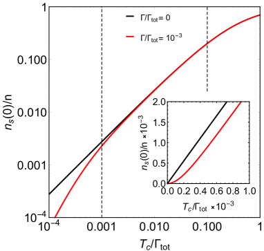
Figure 2: Superfluid fraction $n_{s}(0)/n$ for a series of Dynes superconductors with varying $T_{c}$. The total scattering rate $\Gamma_{\rm tot}=\Gamma_{s}+\Gamma$ is kept fixed and two pair-breaking scattering rates $\Gamma\ll\Gamma_{\rm tot}$ are considered. Three regimes are visible, separated by the vertical dashed lines: clean regime with $\Gamma_{\rm tot}\lesssim T_{c}$, the Homes regime $\Gamma\lesssim T_{c}\lesssim\Gamma_{\rm tot}$, and the novel pair-breaking regime $T_{c}\lesssim\Gamma$.

IV Modified Homes’ law

Superconductivity often occurs in the vicinity of quantum critical points. The observed dome-like shapes of the phase diagrams are then usually explained by the assumption that the pairing strength decreases with distance from the critical point. The control parameter measuring this distance may be pressure, or - as in the case of the cuprates - doping. Recently, Božović et al. have studied the scaling of the low-temperature value of the superfluid density $n_{s}(0)$ with $T_{c}$ in overdoped cuprates.Bozovic16 They have found that when the doping was increased, i.e. when the coupling constant and $T_{c}$ decreased, $n_{s}(0)$ went down, initially following the Homes lawDordevic13 $n_{s}(0)/n\propto T_{c}/\Gamma_{\rm tot}$, but when $T_{c}$ dropped below $\sim 10$ K, a different scaling $n_{s}(0)/n\propto(T_{c}/\Gamma_{\rm tot})^{2}$ was observed.Bozovic16

At first sight, the vanishing of $n_{s}(0)$ looks mysterious, since in a clean system the superfluid density should be given by the density of electrons $n$, which obviously does not vanish in the samples studied by Božović et al. In a clean system, one should therefore expect that $n_{s}(0)=n$ holds for all samples with a finite critical temperature $T_{c}$, and $n_{s}(0)$ should jump discontinuosly (!) to zero when $T_{c}=0$. However, in any real sample, disorder is present. This implies that, when the critical temperature enters the range $T_{c}\lesssim\Gamma_{\rm tot}=\Gamma_{s}+\Gamma$, the sample is in the dirty limit and the Homes scaling

$$\frac{n_{s}(0)}{n}\approx\frac{\pi}{2}\frac{\Delta(0)}{\Gamma_{\rm tot}}$$ (15)

or $n_{s}(0)\propto T_{c}$ should apply, resulting in a smooth development of $n_{s}(0)$ across the superconductor to normal metal transition.

In Fig. 2 the superfluid fraction $n_{s}(0)/n$ for a series of Dynes superconductors with varying coupling strength $g$, but fixed scattering rates $\Gamma$ and $\Gamma_{\rm tot}$, is plotted as a function of their transition temperature $T_{c}$, making use of the explicit formula for $n_{s}(0)/n$ given in Ref. Herman17b, . In order to emphasize the power-law behavior, the log-log plot is used; the curve for $\Gamma=0$ coincides with the result of Ref. Kogan13, . As expected, in the intermediate range of temperatures $\Gamma\lesssim T_{c}\lesssim\Gamma_{\rm tot}$ the Homes scaling Eq. (15) does apply. However, it turns out - see also Eq. (11) - that very close to the superconductor - normal metal transition, there exists yet another regime, $T_{c}\lesssim\Gamma$, where the Homes scaling is replaced by

$$\frac{n_{s}(0)}{n}\approx\frac{\Delta^{2}(0)}{\Gamma_{\rm tot}\Gamma}$$ (16)

and therefore $n_{s}(0)\propto T_{c}^{2}$, exactly as observed in overdoped cuprates by Božović et al. A similar result has been obtained previously,Kogan13b but in that work only weak impurity scattering was considered and the Born approximation was used.

One should note that the result Eq. (16) obviously can not be directly applied to the cuprates with d-wave pairing symmetry. On the other hand, since any real samples should exhibit a finite (although probably small) value of the pair-breaking rate $\Gamma$, the anomalous scaling $n_{s}(0)\propto T_{c}^{2}$ in the immediate vicinity of the superconductor - normal metal transition should be generic.

V Conclusions

In this paper we have dealt with the recently introduced Dynes superconductors, i.e. with superconductors with simultaneously present pair-conserving and pair-breaking scattering processes with rates $\Gamma_{s}$ and $\Gamma$, described by the Green’s function given by Eqs. (2,3).

First we have demonstrated, following the classic work by Janiš,Janis89 that the theory of the Dynes superconductors is thermodynamically consistent, since the CPA equations on which it is based can be derived from a free-energy functional of the self-energy.

We have derived a convenient expression for the free energy difference between the superconducting and the normal state, Eq. (10), and we have shown that it respects Anderson’s theorem. Making use of Eq. (10), we have calculated the electronic specific heat and the thermodynamic critical field of the Dynes superconductors.

Our main result is that the gap parameter, specific heat, critical field, and penetration depth of the Dynes superconductors exhibit power-law scaling with temperature in the low-temperature limit. These results follow from the gapless nature of the Dynes superconductors and they should be readily falsifiable by experiments.

Close to $T_{c}$, we have constructed the Ginzburg-Landau functional for the Dynes superconductors. Our most interesting observation is that (at least in this region of temperatures) the two types of scattering processes influence the upper critical field $H_{c2}$ in exactly opposite ways: In agreement with textbook results, the pair-conserving processes lead to an increase of $H_{c2}$, essentially due to a suppressed sensibility of the electrons to magnetic field. On the other hand, pair-breaking processes lead to a suppression not only of the thermodynamic critical field $H_{c}$ and of the lower critical field $H_{c1}$, but also of $H_{c2}$.

We have also shown that, in the immediate vicinity of a coupling constant-controlled superconductor to normal metal transition, the Homes law Eq. (15) is generically replaced by the pair-breaking dominated scaling law Eq. (16). Although a similar result has in fact been found recently in overdoped cuprates,Bozovic16 our theory does not apply directly to that experiment, since the cuprates are d-wave superconductors, whereas our theory considers s-wave pairing symmetry. Nevertheless, we speculate that the distinction between pair-conserving (small-angle) and pair-breaking (large-angle) scattering might play a role in the experiment of Božović et al. At least the starting point seems to work: small-angle scattering is known to dominate over the large-angle scattering in the cuprates.Herman17 ; Reber12 ; Hong14 However, a serious analysis of the results of Ref. Bozovic16, is beyond the scope of this work.

Appendix A Calculation of $\delta{\cal F}$

In this Appendix we will show that the contributions of the second and of the third terms in Eq. (4) to $\delta{\cal F}$ of a Dynes superconductor can be neglected. To this end, let us first note that the local Green’s function of a Dynes superconductor is given byHerman16

$$\hat{\cal G}_{n}^{-1}=\frac{1}{\pi N_{0}}\frac{i\omega_{n}\tau_{0}-\Delta_{n}\tau_{1}}{\sqrt{\omega_{n}^{2}+\Delta_{n}^{2}}},$$

and the corresponding normal-state local Green’s function obtains from the same expression by setting $\Delta_{n}=0$.

Let us start by considering the contribution of the second term in Eq. (4) to the free energy. Making use of the identity

$${\rm Tr}\ln(A\tau_{0}+B\tau_{1}+C\tau_{3})=\ln(A^{2}-B^{2}-C^{2})$$ (17)

one checks readily that this contribution is the same in both, the normal and the superconducting states. Therefore the second term in Eq. (4) does not contribute to $\delta{\cal F}$.

Thus we are left with the contribution of the third term to $\delta{\cal F}$. Making use of Eq. (17), this can be written as

$$-T\sum_{n}\left\langle\ln\left[1+2\left(\frac{|\omega_{n}|}{\sqrt{\omega_{n}^{2}+\Delta_{n}^{2}}}-1\right)\frac{(1-\pi N_{0}\Gamma_{s})(i\lambda-\pi N_{0}\Gamma)}{\mu^{2}+(1-\pi N_{0}\Gamma_{\rm tot}+i\lambda)^{2}}\right]\right\rangle,$$ (18)

where we have introduced dimensionless pair-conserving and pair-breaking fields $\mu=\pi N_{0}U$ and $\lambda=\pi N_{0}V$, respectively. We remind that the angular brackets denote averaging with respect to the random fields $U$ and $V$. In deriving Eq. (18), we have assumed that the pair-breaking distribution function $P_{m}(V)$ is even. Noting that the expression in round brackets under the logarithm is proportional to $\Delta^{2}$, Eq. (18) can be written, to order $\Delta^{2}$, in the form

$$-2T\sum_{n}\left(\frac{|\omega_{n}|}{\sqrt{\omega_{n}^{2}+\Delta_{n}^{2}}}-1\right)\left\langle\frac{(1-\pi N_{0}\Gamma_{s})(i\lambda-\pi N_{0}\Gamma)}{\mu^{2}+(1-\pi N_{0}\Gamma_{\rm tot}+i\lambda)^{2}}\right\rangle.$$ (19)

A simple integration in complex plane shows that, for a Lorentzian distribution of the pair-breaking field $V$ with width $\Gamma$, and for not too strong disorder, $\pi N_{0}\Gamma_{\rm tot}<1$, the average in Eq. (19) vanishes. This means that the expression Eq. (18) is proportional at least to $\Delta^{4}$ and therefore clearly negligible with respect to the result Eq. (10), as claimed in the main text.

Appendix B Sommerfeld-like expansion

In this Appendix we will derive the Sommerfeld-like expansion. Let us start by observing that we can always split the frequency integral of any function $F(\omega)$ into the following sum of integrals:

$$\int_{0}d\omega F(\omega)=\sum_{n=0}\int_{2\pi Tn}^{2\pi T(n+1)}d\omega F(\omega).$$

If the temperature $T$ is small, then the interval $\langle 2\pi Tn,2\pi T(n+1)\rangle$ is short and we can calculate the corresponding integral by Taylor expansion of $F(\omega)$ around the center of the interval, which happens to coincide with the fermionic Matsubara frequency $\omega_{n}=(2n+1)\pi T$. This way we obtain, to order $T^{4}$,

$$\int_{2\pi Tn}^{2\pi T(n+1)}d\omega F(\omega)=2\pi T\left[F(\omega_{n})+\frac{\pi^{2}}{6}T^{2}F^{\prime\prime}(\omega_{n})\right].$$

Note that even powers of $T$ do not enter this expansion. Summing these results and restoring the upper limit of integration we obtain

$$\int_{0}^{\Omega}d\omega F(\omega)=2\pi T\sum_{\omega_{n}>0}^{\Omega}\left[F(\omega_{n})+\frac{\pi^{2}}{6}T^{2}F^{\prime\prime}(\omega_{n})\right].$$ (20)

Since the sum on the right-hand side contains $\propto T^{-1}$ terms, Eq. (20) represents the integral to order $T^{3}$.

At this point it is sufficient to realize that, to order $T$, the same argument leads to the result

$$\int_{0}^{\Omega}d\omega F^{\prime\prime}(\omega)=2\pi T\sum_{\omega_{n}>0}^{\Omega}F^{\prime\prime}(\omega_{n}).$$ (21)

If we make use of the result Eq. (21) on the right-hand side of Eq. (20), after a trivial manipulation we finally arrive at the Sommerfeld-like expansion, valid to order $T^{3}$,

$$2\pi T\sum_{\omega_{n}>0}^{\Omega}F(\omega_{n})=\int_{0}^{\Omega}d\omega F(\omega)+\frac{\pi^{2}}{6}T^{2}\left[F^{\prime}(0)-F^{\prime}(\Omega)\right].$$

Note that usually $F^{\prime}(\Omega)$ can be neglected, and therefore a finite $T^{2}$ correction is present only if $F^{\prime}(0)$ does not vanish. Since $F(\omega)$ is typically an even function, this means that a finite $T^{2}$ correction results only if $F(\omega)$ is non-analytic at $\omega=0$. This is indeed the case for the Dynes superconductors with a finite value of the pair-breaking scattering rate $\Gamma$. For the sake of completeness let us note that for some quantities, $F^{\prime}(0)$ may be finite also in the clean BCS case. For example, this is the case for $\delta{\cal F}$, see Eq. (10).

The low-temperature expansions presented in Section III.A are obtained by repeated use of the Sommerfeld-like expansion. For the sake of completeness let us mention that the dimensionless coefficient $\kappa$ which appears in the expansion of the superfluid fraction is given by the expression

$$\kappa=\frac{\Delta_{00}}{\Delta(0)}\arctan\left(\frac{\Delta(0)}{\Gamma}\right)+\frac{\Delta_{00}}{\Delta_{00}-\Gamma}+\left(\frac{\Delta(0)}{\Delta_{00}-\Gamma}\right)^{2}.$$

References

- (1) R. C. Dynes, V. Narayanamurti, and J. P. Garno, Phys. Rev. Lett. 41, 1509 (1978).
- (2) Y. Noat, V. Cherkez, C. Brun, T. Cren, C. Carbillet, F. Debontridder, K. Ilin, M. Siegel, A. Semenov, H.-W. Hübers, and D. Roditchev, Phys. Rev. B 88, 014503 (2013).
- (3) P. Szabó, T. Samuely, V. Hašková, J. Kačmarčík, M. Žemlička, M. Grajcar, J. G. Rodrigo, and P. Samuely, Phys. Rev. B 93, 014505 (2016).
- (4) F. Herman and R. Hlubina, Phys. Rev. B 94, 144508 (2016).
- (5) F. Herman and R. Hlubina, Phys. Rev. B 95, 094514 (2017).
- (6) F. Herman and R. Hlubina, Phys. Rev. B 96, 014509 (2017).
- (7) T. Kondo, W. Malaeb, Y. Ishida, T. Sasagawa, H. Sakamoto, Tsunehiro Takeuchi, T. Tohyama, and S. Shin, Nat. Commun. 6, 7699 (2015).
- (8) Julian Simmendinger, Uwe S. Pracht, Lena Daschke, Thomas Proslier, Jeffrey A. Klug, Martin Dressel, Marc Scheffler, Phys. Rev. B 94, 064506 (2016).
- (9) I. Božović, X. He, J. Wu, and A.T. Bollinger, Nature 536, 309 (2016).
- (10) S.V. Dordevic, D.N. Basov, and C.C. Homes, Sci. Rep. 3, 1713 (2013).
- (11) V. Janiš, Phys. Rev. B 40, 11 331 (1989).
- (12) At this point it is convenient to consider a complex pairing field , and to treat and as independent. Equation (6) obtains by minimization with respect to . In the rest of this paper we work in a gauge where the pairing field is real. The frequency cutoff in Eq. (6) has been introduced by hand.
- (13) We have made use of the identity Eq. (17).
- (14) J. Bardeen and M. Stephen, Phys. Rev. 136, A1485 (1964).
- (15) P. W. Anderson, J. Phys. Chem. Solids 11, 26 (1959).
- (16) Note that exhibits the same low-temperature behavior in both, the Dynes and the BCS superconductors, see Appendix B.
- (17) M. Tinkham, Introduction to Superconductivity, 2nd ed. (Dover, New York, 2004).
- (18) V.G. Kogan, Phys. Rev. B 87, 220507(R) (2013).
- (19) V.G. Kogan, R. Prozorov, and V. Mishra, Phys. Rev. B 88, 224508 (2013).
- (20) T. J. Reber, N.C. Plumb, Z. Sun, Y. Cao, Q. Wang, K. McElroy, H. Iwasawa, M. Arita, J. S. Wen, Z. J. Xu, G. Gu, Y. Yoshida, H. Eisaki, Y. Aiura, and D. S. Dessau, Nat. Phys. 8, 606 (2012).
- (21) S.H. Hong, J.M. Bok, W. Zhang, J. He, X.J. Zhou, C.M. Varma, and H.Y. Choi, Phys. Rev. Lett. 113, 057001 (2014).