Broken detailed balance and non-equilibrium dynamics in living systems

Abstract

Living systems operate far from thermodynamic equilibrium. Enzymatic activity can induce broken detailed balance at the molecular scale. This molecular scale breaking of detailed balance is crucial to achieve biological functions such as high-fidelity transcription and translation, sensing, adaptation, biochemical patterning, and force generation. While biological systems such as motor enzymes violate detailed balance at the molecular scale, it remains unclear how non-equilibrium dynamics manifests at the mesoscale in systems that are driven through the collective activity of many motors. Indeed, in several cellular systems the presence of non-equilibrium dynamics is not always evident at large scales. For example, in the cytoskeleton or in chromosomes one can observe stationary stochastic processes that appear at first glance thermally driven. This raises the question how non-equilibrium fluctuations can be discerned from thermal noise. We discuss approaches that have recently been developed to address this question, including methods based on measuring the extent to which the system violates the fluctuation-dissipation theorem. We also review applications of this approach to reconstituted cytoskeletal networks, the cytoplasm of living cells, and cell membranes. Furthermore, we discuss a more recent approach to detect actively driven dynamics, which is based on inferring broken detailed balance. This constitutes a non-invasive method that uses time-lapse microscopy data, and can be applied to a broad range of systems in cells and tissue. We discuss the ideas underlying this method and its application to several examples including flagella, primary cilia, and cytoskeletal networks. Finally, we briefly discuss recent developments in stochastic thermodynamics and non-equilibrium statistical mechanics, which offer new perspectives to understand the physics of living systems.

I Introduction

Living organisms are inherently out of equilibrium. A constant consumption and dissipation of energy results in non-equilibrium activity, which lies at the heart of biological functionality: internal activity enables cells to accurately sense and adapt in noisy environments Lan et al. (2012); Mehta and Schwab (2012), and it is crucial for high-fidelity DNA transcription and for replication Hopfield (1974); Murugan et al. (2012). Non-equilibrium processes also enable subcellular systems to generate forces for internal transport, structural organization and directional motion Needleman and Brugues (2014); Fletcher and Mullins (2010); Brangwynne et al. (2008a); Juelicher et al. (2007); Cates (2012). Moreover, active dynamics can also guide spatial organization, for instance, through nonlinear reaction-diffusion patterning systems Huang et al. (2003); Frey et al. (2017); Halatek and Frey (2012). Thus, non-equilibrium dynamics is essential to maintain life in cells Bialek (2012).

Physically, cells and tissue constitute a class of non-equilibrium many-body systems termed active living matter. However, cellular systems are not driven out of equilibrium by external forces, as in conventional active condensed matter, but rather internally by enzymatic processes. While much progress has been made to understand active behavior in individual cases, the common physical principles underlying emergent active behavior in living systems remain unclear. In this review, we primarily focus on research efforts that combine recent developments in non-equilibrium statistical mechanics and stochastic thermodynamics Seifert (2012); Ritort (2008); Van den Broeck and Esposito (2015) (see Section III) together with techniques for detecting and quantifying non-equilibrium behavior MacKintosh and Schmidt (2010) (see Section II and IV). For phenomenological and hydrodynamic approaches to active matter, we refer the reader to several excellent reviews Marchetti et al. (2013); Ramaswamy (2010); Joanny and Prost (2009); Prost et al. (2015).

Figure 1: A) In thermodynamic equilibrium, transitions between microscopic states are pairwise-balanced, precluding net flux among states. B) Non-equilibrium steady states can break detailed balance and exhibit flux loops. C) Snapshots of an isolated Chlamydomonas flagellum’s beat cycle together with the 3D probability flux map of flagellar dynamics in a coarse grained phase space spanned by the first three modes. Adapted from Battle et al. (2016).

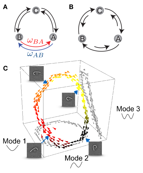
A characteristic feature of living systems is that they are driven out of equilibrium at the molecular scale. For instance, metabolic processes, such as the citric acid cycle in animals and the Calvin cycle for carbon fixation in plants, generally involve driven molecular reaction cycles. Such closed-loop fluxes break detailed balance, and are thus forbidden in thermodynamic equilibrium (Fig. 1A, B) Zia and Schmittmann (2007). Similar directed chemical cycles also power reaction-diffusion patterning systems in cells Frey et al. (2017) and molecular motors, including myosins or kinesins Ajdari et al. (1997). Indeed, such molecular motors can generate mechanical force by coupling the hydrolysis of adenosine triphosphate (ATP) to conformational changes in a mechano-chemical cycle Ajdari et al. (1997); Howard (2001). The dissipation of this chemical energy drives unidirectional transitions between molecular states in this cycle. Such unbalanced transitions break detailed balance and result in directional motion of an individual motor.

One of the central theoretical challenge in the field of active living matter is to understand how the non-equilibrium dynamics of individual molecular components act in concert to drive collective non-equilibrium behavior in large interacting systems, which in general is made of both active and passive constitutents. Motor activity may drive sub-components of cells and tissueMacKintosh and Schmidt (2010); Bausch and Kroy (2006); Glaser and Kroy (2010), but it remains unclear to what extent this activity manifests in the dynamics at large scales. Interestingly, even for systems out of equilibrium, broken detailed balance, for instance, does not need to be apparent at the supramolecular scale. In fact, at large scales, specific driven systems may even effectively regain thermodynamic equilibrium and obey detailed balance Egolf (2000); Rupprecht and Prost (2016).

There are, of course, ample examples where the dynamics of a living system is manifestly out of equilibrium, such as cell division or cell migration. In many cellular systems, however, one can observe stationary stochastic processes that appear at first glance thermally driven. Indeed, for many macromolecular assemblies in cells such as chromosomes Weber et al. (2012), the nucleus Almonacid et al. (2015), the cytoplasm Brangwynne et al. (2009, 2011); Fakhri et al. (2014), membranes Betz et al. (2009); Turlier et al. (2016); Ben-Isaac et al. (2011); Tuvia et al. (1997); Monzel et al. (2015), primary cilia Battle et al. (2015, 2016), and tissue Fodor et al. (2015a) it has been debated to what extent non-equilibrium processes dominate their dynamics. Such observations raise the fundamental and practical question how one can distinguish non-equilibrium dynamics from dynamics at thermal equilibrium. To address this question, a variety of methods and approaches have been developed to detect and quantify non-equilibrium in biological systems. When active and passive microrheology are combined, one can compare spontaneous fluctuations to linear response functions, which are related to each other through the Fluctuation-Dissipation theorem (FDT) when the system is at thermal equilibrium Lau et al. (2003); Mizuno et al. (2007, 2008); Guo et al. (2014). Thus, the extent to which a system violates the FDT can provide insight into the non-equilibrium activity in a system. We will discuss this approach in detail in section II. Other methods employ temperature or chemical perturbations to test the extent to which thermal or enzymatic activities primarily drive the behavior of a system, but such experiments are invasive and are often difficult to interpret. More recently, a non-invasive method to discriminate active and thermal fluctuations based on detecting broken detailed balance was proposed to study the dynamics of mesoscopic systems. This new approach has been demonstrated for isolated flagella (see Fig. 1C) and primary cilia on membranes of living cells Battle et al. (2016). The ideas underlying this method will be detailed in section IV after briefly reviewing related work in stochastic thermodynamics in Sec. III.

Additional important insights on the collective effects of internal activity came from studies on a host of simple reconstituted biological systems. Prominent examples include a variety of filamentous actin assemblies, which are driven internally by myosin molecular motors. Two-dimensional actin-myosin assays have been employed to study emergent phenomena, such as self-organization and pattern formation Schaller et al. (2010, 2011a). Moreover, actin-myosin gels have been used as model systems to study the influence of microscopic forces on macroscopic network properties in cellular components Mizuno et al. (2007); Soares e Silva et al. (2011); Murrell and Gardel (2012); Alvarado et al. (2013); Lenz (2014). Microrheology experiments in such reconstituted actin cytoskeletal networks have revealed that motor activity can drastically alter the rigidity of actin networks Koenderink et al. (2009); Sheinman et al. (2012); Broedersz and MacKintosh (2011) and significantly enhance fluctuations Brangwynne et al. (2008b); Mizuno et al. (2007). Importantly, effects of motor forces observed in-vitro, have now also been recovered in their native context, the cytoplasm Brangwynne et al. (2008b); Guo et al. (2014); Fakhri et al. (2014) and membranes Betz et al. (2009); Turlier et al. (2016). Further experimental and theoretical developments have employed fluorescent filaments as multiscale tracers, which offer a spectrum of simultaneously observable variables: their bending modes Aragon and Pecora (1985); Gittes et al. (1993); Brangwynne et al. (2007a). The stochastic dynamics of these bending modes can be exploited to study non-equilibrium behavior by looking for breaking of detailed balance or breaking of Onsager symmetry of the corresponding correlations functions Gladrow et al. (2016, 2017). This approach will be discussed further in section IV.3.

II Non-equilibrium activity in biological systems and the Fluctuation-Dissipation theorem

Over the last decades, a broad variety of microrheological methods have been developed to study the stochastic dynamics and mechanical response of soft systems. Examples of such systems include synthetic soft matter Cicuta and Donald (2007); Mason et al. (1997); MacKintosh and Schmidt (1999); Waigh (2005); Levine and Lubensky (2000), reconstituted biological networks  Jensen et al. (2015); Bausch and Kroy (2006); Lieleg et al. (2007, 2010); Mahaffy et al. (2000); Gardel et al. (2003); Tseng et al. (2002); Keller et al. (2003); Uhde et al. (2004), as well as cells, tissue, cilia and flagella Mizuno et al. (2007); Prost et al. (2015); Battle et al. (2016); Wilhelm (2008); Fabry et al. (2001); Tseng et al. (2002); Bausch et al. (1999); Ma et al. (2014). In this section, we discuss how the combination of passive and active microrheology can be used to probe non-equilibrium activity in soft living matter. After briefly introducing the basic framework and the most commonly used microrheological techniques, we will discuss a selection of recent studies employing these approaches in conjunction with the fluctuation-dissipation theorem to quantify non-equilibrium dynamics.

Figure 2: The fluctuation dissipation theorem implies a relation between thermal forces exerted by the molecules of the fluid on a Brownian bead and drag forces due to the viscosity of the fluid. A) Cartoon of a freely diffusing Brownian particle. B) Mean square displacement of the particle obtained by performing a Brownian simulation (black), and comparison with the analytical value $<(x(t)-x(0))^{2}>=2Dt$ (red). C) Schematic of an external force $f$ in the positive $x$ direction applied on the particle via an optical tweezer. D) The average displacement for the driven particle (black), obtained from Brownian simulation, increases linearly with time, as $<x(t)-x(0)>=\mu ft$, where $\mu$ is the mobility. In this simple cases, the FDT reduces to the Einstein relation: $D=\mu k_{\rm B}T$.

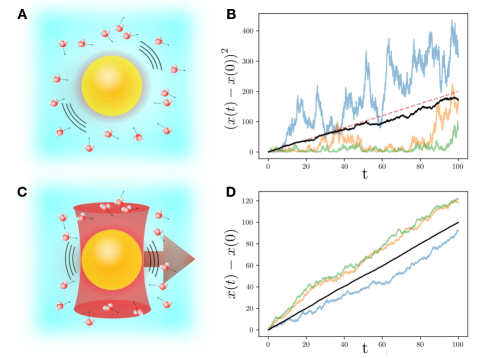
Microscopic probes embedded in soft viscoelastic environments can not only be used to retrieve data about the spontaneous fluctuations of the surrounding medium, but can also be employed to measure the mechanical response of this medium to a weak external force. In the absence of an applied force, the average power spectrum $S_{x}(\omega)=\langle|\Delta x^{2}(\omega)|\rangle$ of fluctuations in the bead position $x(t)$ can be directly measured. The brackets here indicate an ensemble average. The same bead can, in principle, be used to extract the linear response function $\chi_{x}(\omega)=\langle\Delta x(\omega)\rangle/f(\omega)$ by measuring the average displacement induced by a small applied force $f(\omega)$. In systems at thermal equilibrium, these two quantities are related through the Fluctuation-Dissipation theorem (FDT), derived in the context of linear response theory Callen and Welton (1951); Kubo (1966) (see Fig. 2). In frequency space, the FDT relates the autocorrelation function of position fluctuations of an embedded probe particle, in the absence of external forces, to the imaginary part of the associated response function:

$$S_{x}(\omega)=\frac{2k_{B}T}{\omega}\chi^{\prime\prime}_{x}(\omega)\,,$$ (1)

Importantly, a system that is actively driven into a non-equilibrium steady-state will typically not satisfy this equality; this fact can be used to our advantage to study activity in such a system. Indeed, the violation of the FDT has proven to be a useful method to assess the stochastic non-equilibrium nature of biological systems, for instance, by providing direct access to the active force spectrum in cells Guo et al. (2014).

One of the first efforts to investigate deviations from the FDT in a biological system was performed on hair bundles present in the aural canal of a frog Martin et al. (2001). Hair bundles are thought to be primarily responsible for the capability of the ear to actively filter external inputs and emit sound Martin et al. (2001); Van Dijk et al. (2011). To trace the dynamics of the hair bundle, a flexible glass fiber was attached to the bundle’s tip to measure both the position autocorrelation function and the associated response to periodic external stimuli. Interestingly, the magnitude of position fluctuations was observed to largely exceed the linear-reponse-based levels for a purely thermal system. This violation of the FDT indicates the presence of an internal energy source driving the system out of equilibrium.

A suggested measure of the degree of violation of the FDT is a frequency-dependent “effective temperature” $T_{\rm eff}(\omega)$Cugliandolo et al. (1997); Cugliandolo (2011); Loi et al. (2008); Bursac et al. (2005); Martin et al. (2001); Prost et al. (2009); Wilhelm (2009), defined as the ratio between fluctuations and dissipation: $T_{\rm eff}(\omega)\equiv\omega\,S_{x}(\omega)/2k_{B}\chi_{x}^{\prime\prime}(\omega)$. For a system at thermal equilibrium $T_{\rm eff}=T$. However, this quantity can be drastically modified for an actively driven bundle: Close to its spontaneous oscillation frequency of $\omega_{0}$, the imaginary part of the response function of the hair bundle becomes negative. This implies that $T_{\rm eff}$ is frequency dependent and can also assume negative values.

Even though this example illustrates how the dimensionless quantity $T_{\rm eff}/T$ provides a simple metric for non-equilibrium, the concept of an effective temperature in this context remains a topic of debate  Ben-Isaac et al. (2011); Fodor et al. (2016); Turlier et al. (2016); Martin et al. (2001); Fodor et al. (2015b). Note, the existence of an effective temperature should not be mistaken for the existence of a physical mapping between an active system and an equilibrium at a temperature $T_{\rm eff}$. While there certainly are examples where such a mapping exists, this will not be the case in general. Furthermore, it is not obvious how to interpret negative or frequency dependent effective temperatures, but an interesting perspective is offered by Cugliandolo et al. Cugliandolo et al. (1997). They demonstrated for a class of systems that the effective temperature can indicate the direction of heat flow and acts as a criterion for thermalization Cugliandolo et al. (1997). In a more recent study, the conditions were derived for systems in non-equilibrium steady states to be governed by quasi-FDT: a ralation similar to the equilibrium FDT, but with the temperature replaced by a constant $T_{\rm eff}>T$Dieterich et al. (2015). These conditions entail that the intrinsic relaxation time of the system is much longer than the characteristic time scale of the active forces. However, these conditions may become more complicated by systems with a viscoelastic response governed by a spectrum of timescales for which the thermal force spectrum is colored Chaikin and Lubensky (1995). Beyond being a simple way of measuring deviations from the FDT, the concept of an effective temperatures may thus provide insight into active systems, but this certainly requires further investigation. Alternative measures for non-equilibrium have been the subject of more recent developments based on phase spaces currents and entropy productions rates, which are discussed in sections III and IV.

II.1 Active and passive microrheology

The successful application of the FDT in an active unidimensional context like the case of the hair bundle described above, paved the road for new approaches: microscopic probes were embedded into increasingly more complex biological environments to study the mechanics and detect activity inside reconstituted cytoskeletal systems Gardel et al. (2003); Bausch and Kroy (2006); Lau et al. (2003); Mizuno et al. (2007) and living cells Fabry et al. (2001); Yamada et al. (2000); Lau et al. (2003).

Probing violations of the FDT in such soft biological systems relies on high-precision microrheological approaches. Conventional single particle microrheology is divided into two categories: passive microrheology (PMR) Mason and Weitz (1995) and active microrheology (AMR) Ziemann et al. (1994); Amblard et al. (1996); Schmidt et al. (1996). PMR depends on the basic assumption that both the FDT and the generalized Stokes-Einstein relationship apply. This assumption ensures that a measurement of the position fluctuation spectrum directly yields the rheological properties of the medium. Indeed, the generalized Stokes-Einstein relation connects the force-response function to the viscoelastic response of the medium Mason and Weitz (1995),

$$\chi_{x}(\omega)=\frac{1}{6\pi aG(\omega)}\,,$$ (2)

where $a$ is the radius of the bead. This equation is valid in the limit of Stokes’ assumptions, i.e. overdamped spherical particle embedded in a homogeneous incompressible continuum medium with no slip boundary conditions at the particle’s surface. Here, $G(\omega)=G^{\prime}(\omega)+iG^{\prime\prime}(\omega)$ describes the complex shear modulus, where the the real part is the storage modulus $G^{\prime}$ describing the elastic component of the rheological response, and the imaginary part, $G^{\prime\prime}$, is the loss modulus accounting for the dissipative contribution. Under equilibrium conditions, the imaginary part of the response function $\chi_{x}^{\prime\prime}$ is also related to the position power spectral density via the FDT (Eq. (1)). Thus, in PMR, the response function and the shear modulus are measured by monitoring the mean square displacement (MSD) $\langle\Delta x^{2}\rangle(t)\equiv\langle(x(t)-\langle x\rangle)^{2}\rangle$ of the embedded beads. By contrast, in AMR the mechanical response is directly assessed by applying an external force on an embedded probe particle, usually by means of optical traps or magnetic tweezers. Within the linear response regime, the response function can be measured as $\chi_{x}=\langle\Delta x(\omega)\rangle/f(\omega)$, and the complex shear modulus can then be determined from the generalized Stokes-Einstein relation (Eq. (2)).

Although one-particle PMR has proven to be a useful tool to determine the equilibrium properties of homogeneous systems, biological environments are typically inhomogeneous. Such intrinsic inhomogeneity can strongly affect the local mechanical properties  Beroz et al. (2017); Jones et al. (2015), posing a challenge to determine the global mechanical properties using microrheology. To circumvent this issue, two-point particle microrheology is employed Crocker et al. (2000); Lau et al. (2003). This method is conceptually similar to one-point microrheology, but it is based on a generalized Stokes-Einstein relation for the cross-correlation of two particles at positions ${\bf r}_{1}$ and ${\bf r}_{2}$ with a corresponding power spectral density $S_{{r}_{1},{r}_{2}}(R,\omega)$ with $R=|{\bf r}_{2}-{\bf r}_{1}|$. This correlation function depends only on the distance between the two particles and on the macroscopic shear modulus of the medium. Thus, $S_{{r}_{1},{r}_{2}}$ is expected to be less sensitive to local inhomogeneities of the medium Crocker et al. (2000).

PMR has been extensively employed to assess the rheology of thermally driven soft materials in equilibrium, such as polymer networks Schnurr et al. (1997); Mizuno et al. (2008); Mason et al. (1997); Addas et al. (2004); Gittes and MacKintosh (1998); Gittes et al. (1997); Mason and Weitz (1995); Chen et al. (2003); Mason (2000), membranes and biopolymer-membrane complexes  Helfer et al. (2000); Fedosov et al. (2010); Turlier et al. (2016), as well as foams and interfaces Lee et al. (2010); Prasad et al. (2006); Ortega et al. (2010). However, a PMR approach cannot be employed by itself to establish the mechanical properties of non-equilibrium systems, for which the FDT generally does not apply. If the rheological properties of the active system are known, the power spectrum of microscopic stochastic forces $\Delta(\omega)$— with both thermal and active contributions — can be extracted directly from PMR data for a single sphere of radius $a$ Lau et al. (2003); Mizuno et al. (2008); Caspi et al. (2000)

$$\Delta(\omega)=6\pi a\,S_{x}(\omega)|G(\omega)|^{2}\,.$$ (3)

The expression for the power spectrum of force fluctuations was justified theoretically Lau et al. (2003); MacKintosh and Levine (2008), considering the medium as a continuous, incompressible, and viscoelastic continuum at large length scales. The results discussed above laid out the foundations for a variety of studies that employed microrheological approaches to investigate active dynamics in reconstituted cytoskeletal networks and live cells, which will be discussed next.

II.2 Activity in reconstituted gels

The cytoskeleton of a cell is a composite network of semiflexible polymers that include microtubules, intermediate filaments, F-actin, as well as associated proteins for cross-linking and force generation Fletcher and Mullins (2010); Alberts et al. (1994); Kasza et al. (2007); Bausch and Kroy (2006). The actin filament network is constantly stretched and displaced by collections of molecular motors such as Myosin II. These motors are able to convert ATP into directed mechanical motion and play a major role in the active dynamics of the cytoskeleton Mizuno et al. (2007); Köhler and Bausch (2012); Stricker et al. (2010); Juelicher et al. (2007); Fakhri et al. (2014).

To develop a systematic and highly controlled platform for studying this complex environment, simplified cytoskeletal modules with a limited number of components were reconstituted in vitro, opening up a new field of study Bausch and Kroy (2006); Jensen et al. (2015); Lin et al. (2007); Kasza et al. . Among these reconstituted systems, F-actin networks are perhaps the most thoroughly examined Lieleg et al. (2010); Mizuno et al. (2007); Gardel et al. (2008); Joanny and Prost (2009); Pelletier et al. (2009); Kasza et al. ; Murrell et al. (2015). Indeed, in the presence of motor activity, these networks display a host of intriguing non-equilibrium behaviors, including pattern formation Soares e Silva et al. (2011); Schaller et al. (2010, 2011a, 2011b), active contractiliy and nonlinear elasticity  Koenderink et al. (2009); Bendix et al. (2008); Ronceray et al. (2016); Murrell and Gardel (2012); Lenz et al. (2012); Wang and Wolynes (2012), as well as motor-induced critical behavior Alvarado et al. (2013); Sheinman et al. (2012).

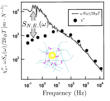
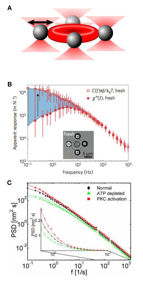
To study the steady state non-equilibrium dynamics of motor-activated gels, Mizuno et al. constructed a three-component in vitro model of a cytoskeleton, including filamentous actin, an actin crosslinker, and Myosin II molecular motors Mizuno et al. (2007). The mechanical properties of the network were determined via AMR, while the activity-induced motion of an embedded particle was tracked via PMR. The measured imaginary component of the mechanical compliance, $\chi_{x}^{\prime\prime}(\omega)$, was compared to the response predicted via the FDT, i.e. $\omega S_{x}(\omega)/2k_{B}T$, as shown in Fig. 3. In the presence of myosin, the fluctuations in the low-frequency regime were observed to be considerably larger than expected from the the measured response function and the FDT, indicating that myosin motors generate non-equilibrium stress fluctuations that rise well above thermally generated fluctuations at low frequencies.

These observations raise the question why motor-driven active fluctuations only dominate at low frequencies. This can be understood from a simple physical picture in which myosin motor filaments bind to the actin network and steadily build up a contractile force during a characteristic processivity time $\tau_{p}$  Howard (2002). After this processivity time, the motor filament detaches from the actin polymers to which they are bound, producing a sudden drop in the force that is exerted locally on the network. Such dynamics generically generate a force spectrum $\Delta(\omega)\sim\omega^{-2}$ MacKintosh and Levine (2008); Levine and MacKintosh (2009), which can dominate over thermally driven fluctuations in an elastic network on time scales shorter than the processivity time (See Sec. II.5 for a more detailed discussion).

Figure 3: Violation of the FDT in reconstituted actin-myosin networks (inset). At frequencies below 10 Hz the response function estimated using the FDT from spontaneous fluctuations of a probe bead deviates significantly from the response $\chi^{\prime\prime}$ measured directly using active microrheology (full circles). Adapted from Mizuno et al. (2007).

In addition to the appearance of non-equilibrium fluctuations, the presence of motors in the network led to a substantial ATP-dependent stiffening. It is well known that crosslinked semiflexible polymer networks stiffen under an external strain  Storm et al. (2005); Gardel (2004); Lieleg et al. (2007); Kasza et al. (2009); Lin et al. (2010). Motors can effectively crosslink the network leading to stiffening, but they can also generate local contractile forces, and it is less clear how internal stress generation from such motor activity can induce large scale stresses and control network stiffness Ronceray et al. (2016); Broedersz and MacKintosh (2011); Shokef and Safran (2012); Ronceray and Lenz (2015); Hawkins and Liverpool (2014); Xu and Safran (2015); MacKintosh and Levine (2008); Chen and Shenoy (2011); Wang and Wolynes (2012). In a more recent experimental study, it was shown that motor generated stresses can induce a dramatic stiffening behavior of semiflexible networks Koenderink et al. (2009). This mechanism could be employed by cells and tissues to actively regulate their stiffness  Shokef and Safran (2012); Tee et al. (2009); Lam et al. (2011); Jansen et al. (2013).

An ensemble of beads dispersed in an active gel can not only be used to obtain fluctuation spectra, but also to infer the full probability distribution of the beads’ displacements at a time-lag $\tau$ Toyota et al. (2011); Stuhrmann et al. (2012); Fodor et al. (2015b). This distribution is typically observed to be Gaussian for a thermal systems, while non-Gaussian tails are often reported for an active system. In actin-myosin gels, for example, exponential tails in the particle position distributions are observed at timescales $\tau$ less than the processivity time of the motors. By contrast, at larger time lags, a Gaussian distributions is observed, in agreement with what was previously found for fluctuation spectra in frequency space Mizuno et al. (2007). Importantly however, non-Gaussianity is not a distinctive trait of non-equilibrium activity, since it can also appear in thermal systems with anharmonic potentials. Moreover, Gaussian distributions could also govern active systems (see Sec. III.1).

The hallmarks of activity discussed above for actin-myosin gels are also observed in synthesized biomimetic motor-driven filament assemblies. Betrand et al. created a DNA-based gel composed of stiff DNA tubes with flexible DNA linkers Bertrand et al. (2012). As an active component, they injected FtsK50C, a bacterial motor protein that can exert forces on DNA. An important difference with the actin-based networks described above, is that here the motors do not directly exert forces on the DNA tubes, which constitute the filaments in the gel. Instead, the motors attach to long double-stranded DNA segments that were designed to act as a cross-linker between two stiff DNA tubes. Upon introduction of the motors, the MSD of tracer beads that were embedded in the gel was strongly reduced, even though the motors act as an additional source of fluctuations. This observation suggests a substantial stiffening of the gel upon motor activation. Furthermore, the power spectrum of bead fluctuations exhibited $\sim\omega^{-2}$ behavior, similar to results for in vitro actin-myosin systems and even for live cells, which we discuss next.

II.3 Activity in cells

The extensive variety of biological functions performed by living cells places daunting demands on their mechanical properties. The cellular cytoskeleton needs to be capable of resisting external stresses like an elastic system to maintain its structural integrity, while still permitting remodelling like a fluid-like system to enable internal transport as well as migration of the cell as a whole Deng et al. (2006); Kasza et al. (2007). The optimal mechanical response clearly depends on the context. An appealing idea is that the cell can use active forces and remodelling to dynamically adapt its (nonlinear) viscoelastic properties in response to internal and external cues Ahmed and Betz (2015); Ehrlicher et al. (2015); Yao et al. (2013). In light of this, it is interesting to note that experiments on reconstituted networks suggest that activity and stresses can lead to responses varying from fluidization to actual stiffening Humphrey et al. (2002); Koenderink et al. (2009); Brangwynne et al. (2008a). Currently, however, it remains unclear how such a mechanical response plays a role in controlling the complex mechanical response of living cells Fletcher and Mullins (2010); Fernández and Ott (2008); Wolff et al. (2012); Krishnan et al. (2009); Deng et al. (2006); Trepat et al. (2007); Ehrlicher et al. (2015).

Important insights into the mechanical response of cell were provided by experiments conducted by Fabry et al. via beads attached to focal adhesions near the cortex of human airway muscle cells. Their data indicate a rheological response where the loss and storage moduli are comparable, with a magnitude roughly in the range 100-1000 Pa around 1 Hz, and depend on frequency as a power law $|G(\omega)|\sim\omega^{x}$ with a small exponent $0.1\leq x\leq 0.3$ Fabry et al. (2001), reminiscent of soft glassy rheology Sollich et al. (1997); Semmrich et al. (2007); Hoffman and Crocker (2009); Bursac et al. (2005); Balland et al. (2006).

The studies conducted by Lau et al. Lau et al. (2003) and Fabry Fabry et al. (2001) employed different probes at different cell sites for active and passive measurements, and determined a diffusive-like spectrum $\langle\Delta x^{2}\rangle\sim\omega^{-2}$. A more recent assessment Wilhelm (2008) was able to measure the cellular response and the fluctuation spectrum with the same probe and at the same cellular location. The rheological measurement of $G$ was found to depend critically on the size of the engulfed magnetic beads and yielded a power law dependence on the applied torque-frequency $G(\omega)\sim\omega^{0.5-0.6}$. Furthermore, the conjuncted PMR and AMR assessments revealed a clear violation of the FDT, with the MSD of the beads increasing super diffusively with time. Measurements of the MSD of micron-size beads located around the nucleus of a living fibroblast also exhibited super-diffusive spectra, with a $\sim t^{3/2}$ dependence Sakaue and Saito (2017). Upon depolymerization of the microtubule network, diffusive behavior was restored suggesting that the rectifying action of microtubule-related molecular motors might be responsible for the super diffusive behavior. Furthermore, when the motors were inhibited without perturbing the polymer network, subdiffusive behavior was observed, in accordance to what is expected in equilibrium for a Brownian particle diffusing in a viscoelastic environment Caspi et al. (2000)

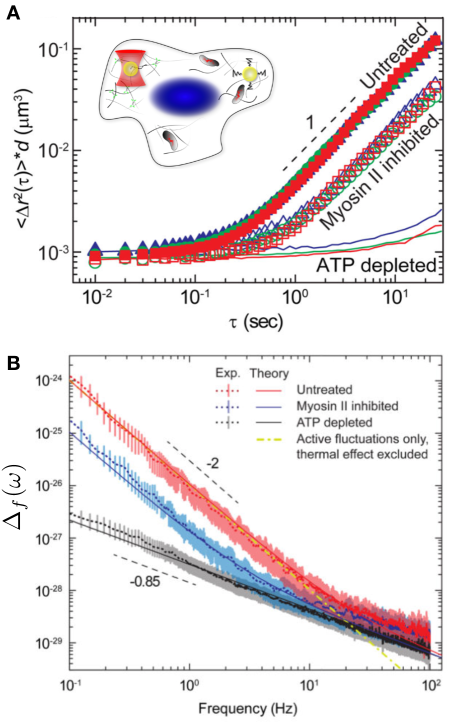
A systematic measurement of both active and passive cytoplasmic properties was carried out by Guo et al. via sub-micron colloidal beads injected into the cytoplasm of live A7 Melanoma cells. The probe beads were conveniently employed to perform both PMR and AMR with the use of optical tweezers. The active microrheology experiments indicated a response with a shear modulus around 1 Pa, softer than measured near the cortex in Fabry et al. (2001), but with a similar power-law dependence of the complex shear modulus on frequency $|G(\omega)|\sim\omega^{0.15}$ Guo et al. (2014). Passive microrheology was employed to measure the mean square displacement (MSD) of position fluctuations under the same conditions in the cytoplasm (Fig. 4A). At short time-scales, the MSD is almost constant, as expected for a particle embedded in a simple elastic medium. By contrast, at long time scales, the system can relax, resulting in an MSD that increases linearly with time, as would be expected for simple diffusion-like behavior of a probe particle in a viscous liquid as was also observed in earlier studies Yamada et al. (2000); Alcaraz et al. (2003)

Although these observations are deceptively close to the features of simple Brownian motion, this is clearly not the correct explanation for this phenomenon, given that the mechanical response of the system measured by AMR is predominantly elastic at these time scales. Furthermore, by treating cells with blebbistatin, an inhibitor of Myosin II, the magnitude of fluctuations notably decreased in the long time regime. While this suggests an important role for motor generated activity in driving the fluctuations of the probe particle, Myosin inhibition could also affect the mechanical properties of the cytoplasm, and thereby also the passive, thermally driven fluctuations of the probe particle. Nonetheless, by combining AMR and PMR it became clear that the system violates the FDT at these long time scales, implying that the system is not only out of equilibrium, but also that non-equilibrium activity can strongly alter the spectrum of force fluctuations.

Figure 4: Fluctuations of probe particles inside living cells. A) The MSD, $\langle\Delta x^{2}(\tau)\rangle$, of tracer beads rescaled by the particle diameter $d$, for untreated, Myosin inhibited, and ATP depleted cells. For untreated cells the MSD shows a plateau at short time scales, after which the MSD increases linearly with time. When Myosin is inhibited by blebbistatin, the power law does not change but the magnitude of the MSD is reduced. By depleting ATP in the cytoplasm, the dependence of the MSD on time becomes consistent with thermal motion in a viscoelastic environment at short time. A cartoon of AMR and PMR performed inside the cytoplasm is shown in the inset. B) Measured force spectrum in the cytoplasm of untreated (red), blebbistatin treated (blue) and ATP-depleted (black) A7 cells. Adapted from Guo et al. (2014).

The combination of AMR and PMR measurements was employed to infer the spectrum of force fluctuations using a method called Force Spectrum Microscopy (FSM). This method makes use of the relation $\Delta(\omega)=|k(\omega)|^{2}\langle\Delta x^{2}\rangle(\omega)$, where the complex spring constant $k\equiv 1/\chi_{x}$ is related to $G$ by $k=6\pi Ga$ (see Eq. (2)). The measured force spectrum exhibited two different power-law regimes: at high frequencies $\Delta(\omega)\sim\omega^{-0.85}$, while at low frequencies ($\omega\lesssim 10$ Hz), $\Delta(\omega)\propto\omega^{-2}$, in agreement with what is expected for typical molecular motor power spectra, as depicted in Fig. 4B.

The observed high-frequency behavior is in accordance with predictions for particle fluctuations driven by thermal forces in a nearly elastic medium. In fact, if $G\sim\omega^{\beta}$, then $\langle\Delta x^{2}\rangle(\omega)\sim\omega^{-(\beta+1)}$ at thermal equilibrium Lau et al. (2003). This implies that $\Delta(\omega)\sim\omega^{-0.85}$, with the measured $\beta=0.15$. By contrast, an active model predicts $\langle\Delta x^{2}\rangle(t)\sim t^{1+2\beta}$ if $\Delta(\omega)\sim\omega^{-2}$, which is consistent with what is observed in reconstituted motorized gels at times shorter than the processivity time $\tau_{p}$  Koenderink et al. (2009); Brangwynne et al. (2008b). These experiments and others Fakhri et al. (2014); Brangwynne et al. (2007b) have thus established the active nature and the characteristics of force spectra in the cytoplasm using embedded beads.

Various experiments employing PMR in live cells have been performed using alternative synthetic probes, such as nanotubes or embedded intracellular entities, including microtubules, vesicles, and fluorescently labeled chromosomal loci. In a recent study, Fakhri et al. developed a new technology to investigate the stochastic dynamics of motor proteins along cytoskeletal tracks Fakhri et al. (2014). This cutting-edge method consists of imaging the near-infrared luminescence of single-walled carbon nanotubes (SWNT) targeted to kinesin-1 motors in live cells. Although traces of moving SWNT show long and relatively straight unidirectional runs, the dependence of the MSD of the tracer particle on time exhibits several powerlaw regimes with an exponent that depends on the time range: At $t\approx 0.1sec$ the exponent transitions from a value around 0.25 at short times to a value of 1 at larger times. By decomposing the MSD in motion along and perpendicular to the microtubule axis, it was shown that the dynamics of SWNT tracers originates from two distinct contributions: directed motion along the microtubules together with transverse non-directed fluctuations. The transverse fluctuations were attributed to bending fluctuations of the stiff microtubules, owing to motor-generated activity in the surrounding cytoskeleton, consistent with prior observationsBrangwynne et al. (2007b). Indeed, the full time dependence of the MSD of traced kinesin motors could be described quantitatively with a model that assumes cytoskeletal stress fluctuations with long correlation times and sudden jumps. This is in agreement with a physical picture in which myosin mini-filaments locally contract the actin network during an attachment time set by the processivity time of the motors, followed by a sudden release.

Active bursts generated by Myosin-V are fundamental for nuclear positioning in mouse oocytes. In fact, active diffusion is here thought to create pressure gradient and directional forces strong enough to induce nuclear displacements Almonacid et al. (2015); Razin et al. (2017a, b). As in the earlier studies discussed above, the FDT is sharply violated at low frequencies, while it is recovered at large ones Ahmed et al. (2015).

To study the steady-state stochastic dynamics of chromosomes in bacteria, novel fluorescence-labelling techniques were employed on chromosomal loci in E.Coli cells. These experiments yielded sub-diffusive MSD behavior: $\langle\Delta x^{2}\rangle(t)\sim t^{0.4}$ Weber et al. (2010, 2012); Sakaue and Saito (2017); Vandebroek and Vanderzande (2015). Although purely thermal forces in a viscoelastic system, such as the cytoplasm or a nucleoid, can also generate sub-diffusive motion MacKintosh (2012), Weber et al. demonstrated a clear dependence of the MSD on ATP levels: When ATP was depleted from the cell, the MSD magnitude was reduced. Surprisingly however, the exponent, $\alpha=0.4$, was not affected by varying ATP levels. Under the assumption that a change in the ATP level does not effect the dynamic shear modulus of the cytoplasm, this could be interpreted as resulting from active forces with a white noise spectrum and shear modulus that scales with frequency as $G\sim\omega^{0.7}$. While these results provide evidence for the existence of active diffusion by chromosomal loci, less invasive and more direct approaches are required to confirm and further study non-equilibrium behavior in the bacterial cytoplasm Parry et al. (2014) and to understand dynamics of the chromosome.

II.4 ATP-dependent elastic properties and membrane fluctuations in red blood cells

The elastic properties of cells play an important role in many biological systems. The unusually high deformability of red blood cells (RBCs) is a prominent example in this respect, lying at the heart of the cardiovascular system. RBCs have the astonishing capability to squeeze through micron-sized holes, which ensures seamless blood flow through tight capillaries. To explore how these astonishing properties emerge, a detailed understanding of passive and active behavior of the membrane enclosing RBCs and its connection to the underlying cytoskeleton is required.

The bending dynamics of membranes are largely determined by their curvature and their response to bending forces thus depends on their local geometry Evans (1983); Granek (1997, 2011); Lin et al. (2006). In flat membranes, the power spectral density of bending fluctuations is expected to scale as $\omega^{-5/3}$ for large $\omega$ Milner and Safran (1987); Betz et al. (2009); Lin et al. (2006). A spectrum close to a $-5/3$-decay has indeed been reported in measurements of red blood cell membrane fluctuations Betz et al. (2009). Interestingly, the same experiments showed decreasing fluctuation amplitudes upon ATP-depletion, possibly indicating the role of non-equilibrium processes. The precise origin and nature of these processes, however, is difficult to determine due to the composite, ATP-dependent structure of erythrocyte membranes and cytoskeleton.

In addition, a flickering motion of RBC membranes observed in in microscopy experiments has sparked a discussion about the origin of these fluctuations. Indeed, the extent to which active processes determine the properties of RBCs is subject of intense research activity  Brochard and Lennon (1975); Strey et al. (1995); Gov (2004); Gov and Safran (2005); Betz et al. (2009); Park et al. (2010); Yoon et al. (2011); Ben-Isaac et al. (2011); Rodríguez-García et al. (2016).

Although myosin is present in the cytoskeleton of human erythrocytes, mechano-chemical motors are not the only source of active forces in the cell. In the membrane of RBCs, actin forms triangular structures with another filamentous protein called spectrin. These structures are linked together by a protein known as 4.1R. Phosphorylation of 4.1R, an ATP-consuming process, causes the spectrin-actin complex to dissociate, which could lead to a softening of the cell. In accordance with this model, ATP-depletion was found to increase cell stiffness Tuvia et al. (1997), and at the same time reduce membrane fluctuations on the $1-10$ s time scale. This is exemplified by the comparison between the green (ATP-depleted) and black (normal conditions) curves in Fig. 5C.

In order to relate the magnitude of fluctuations to membrane stiffness $\kappa$ and tension $\sigma$, Betz et al. Betz et al. (2009) employed a classical bending free-energy Lin et al. (2006)

$$\mathcal{F}\left[h(r)\right] =\int\mathrm{d}^{2}r\,\left[\frac{\kappa}{2}\left(\mathop{}\!\mathbin{\bigtriangleup}h\right)^{2}+\frac{\sigma}{2}\left(\nabla h\right)^{2}\right].$$ (4)

Here, $\kappa$ represents the membrane stiffness and $\sigma$ is the surface tension. A mode decomposition of the transverse displacement $h(\vec{q})$, evolving under thermal equilibrium dynamics of this energy functional leads to the correlator,

$$\langle h(\vec{q},t)h(\vec{q}\ ^{\prime},t^{\prime}))\rangle =\frac{\left(2\pi\right)^{2}k_{B}T}{\kappa q^{4}+\sigma q^{2}}\delta(\vec{q}+\vec{q}\ ^{\prime})e^{-\frac{|t-t^{\prime}|}{\tau_{q}}},$$ (5)

which is reminiscent of the correlator derived for semiflexible filaments (See section IV.3). The decorrelation time $\tau_{q}$ is given by $\tau_{q}=4\eta q/(\kappa q^{4}+\sigma q^{2})$. A Fourier transformation of the correlator yields the theoretical prediction for the power spectral density shown in Fig. 5. This model was also generalized to consider membrane fluctuations in the presence of active forces Gov and Safran (2005); Rodríguez-García et al. (2016); Lin et al. (2006).

The observed stiffening of the membrane upon ATP-depletion, presented a dilemma: membrane stiffening at low ATP could be the cause of the reduction of thermally driven membrane flickering, as apposed to a picture in which membrane flickering is primarily due to stochastic ATP-driven processes. This conundrum was resolved in a subsequent study, in which RBC flickering motion was shown to violate the equilibrium FDT, providing strong evidence for an active origin of the flickering Turlier et al. (2016). To demonstrate this, Turlier et al. Turlier et al. (2016) attached four beads to live erythrocytes, three of them serving as a handle, while the remaining bead can either be driven by a force exerted by optical tweezers or the unforced bead motion can be observed to monitor spontaneous fluctuations. The complex response $\chi_{x}(\omega)$ is then obtained from the ratio of Fourier transformations of the position $x(\omega)$ and force $F(\omega)$. The equilibrium FDT in Eq. (1) relates these two quantities. The measured imaginary response $\chi_{x}^{\prime\prime}(\omega)$ is plotted together with the response calculated from Eq. (1) in Fig. 5B. While the two curves exhibit stark differences at low frequencies, they become comparable for frequencies above 10 $\rm Hz$. Thus, whatever the precise nature of active processes in erythocyte membranes is, the intrinsic timescales of these processes appear to be on the order of $1-10$ Hz.

Figure 5: A) Cartoon of a red blood cell whose membrane conformations and response are tracked via four attached microscopic beads. B) The response and flickering spectrum of a red blood cell differ below 10 Hz, indicating a clear violation of the FDT. Adapted from Turlier et al. (2016). C) Power spectrum of RBC membrane fluctuations under normal conditions (black), after ATP-depletion (green) and after addition of a PKC (red). PKC stands for protein kinase C, which catalyzes the phosphorylation of 4.1R, leading to increased dissociation of actin-spectrin structures. Adapted from Betz et al. (2009).

To explore the contributions to the mechanical properties of the membrane that arise specifically due to phosphorylation of 4.1R (and other molecules) in erythrocytes, the authors devised a semi-analytical non-equilibrium model for the elastic response of the membrane. Phosphorylation events are here modelled as on-off telegraph processes, which are added to an equilibrium description of membrane bending, such as in Eq. (4). The authors then decompose the membrane shape into spherical harmonic modes and calculate the single-mode power spectral density, which reads

$$S_{x}^{lm}(\omega) =\frac{2k_{B}T}{\omega}\chi_{x}^{lm}(\omega)^{\prime\prime}+\frac{2\langle n_{a}\rangle\left(1-\langle n_{a}\rangle\right)\tau_{a}}{1+\omega\tau_{a}}\left|N^{lm}(\omega)\right|^{2},$$ (6)

with $\tau_{a}=(k_{a}+k_{i})^{-1}$ being the timescale, $n_{a}=k_{a}/(k_{a}+k_{i})$ being the phosphorylation activity, and $N^{lm}(\omega)$ capturing the effects of tangential active noise on the membrane shape. The rate coefficients $k_{a}$ and $k_{i}$ characterize the simplified activate-inactivate ($a$-$i$) telegraph model, that the authors employ. Again, the expression in Eq. (6) bears interesting similarities with the power spectrum of filament fluctuations (see Sec. IV.3, Eqs. (49), and (50)). The mode response here in Eq. (6) is also composed of independent thermal and non-equilibrium contributions. Interestingly, the model shows that the curvature of the membrane is crucial for it to sustain active flickering motions. Only a curved surface allows fluctuations of tangential stress to result in transversal motion. Modes that correspond to wavelengths too short to couple to tangential stresses also do not seem to be affected by non-equilibrium processes. The flickering therefore appears to be caused by a coupling of tangential stresses to transversal motion only within a certain window of spherical modes $2\leq l\leq l*$.

ATP-dependent fluctuations seem to contribute directly to the extraordinary mechanic properties of erythrocytes and may even help maintain their characteristic biconcave shape Park et al. (2010). Recently, bending fluctuations of membranes have been implicated in general cell-to-cell adhesion Fenz et al. (2017). The satisfactory agreement of theoretical and experimental fluctuation spectra in the examples discussed above highlights the merit of non-equilibrium statistical approaches to model and indeed explain properties of living biological matter.

The violation of the FDT is an elegant tool for the detection of activity in biological systems, as illustrated by the many examples discussed in the section above. That being said, for such a method to be applicable, the simultaneous measurement of fluctuations and response is required. Even though this method gives information on the rheological properties of the system, its applicability can be challenging in contexts where the system is particularly delicate or poorly accessible such as chromosomes, the cytoskeleton, intracellular organelles, and membranes. Thus, in many cases a less invasive approach might be desired. These alternative approaches are further discussed in section IV.

II.5 Simple model for $\omega^{-2}$ active force spectra in biological systems

As illustrated by the many examples discussed above, the mean square displacement of a probe particle in the cytoskeleton or in a reconstituted motor-activated gel has been widely observed to be surprisingly similar to a diffusive spectrum in a viscous medium: $\langle\Delta x^{2}\rangle\sim t$. In a purely viscous environment, with only Brownian thermal forces, the force spectrum is well-described by white noise, which has a flat power spectrum over the whole frequency range by definition. The magnitude of the complex shear modulus for a purely viscous fluid is $|G|^{2}\sim\omega^{2}$. Such a simple rheological response, taken together with a white noise force spectrum, yields a displacement spectrum $\langle\Delta x^{2}\rangle\sim\Delta/|G|^{2}\sim\omega^{-2}$ at all frequencies. This mechanism however does not explain the effective diffusive behavior measured in cells below 10 Hz  Guo et al. (2014); Fodor et al. (2015b); Brangwynne et al. (2009, 2008a); Gallet et al. (2009); Fakhri et al. (2014). Below, we illustrate with a simple model MacKintosh and Levine (2008); Levine and MacKintosh (2009); Gallet et al. (2009); Osmanović and Rabin (2017); Samanta and Chakrabarti (2016) that any active force with a sufficiently rapid decorrelation time will produce effective diffusive behavior of a bead in an elastic medium.

Consider a particle moving in a simple viscoelastic solid with both active forces, $f_{A}$, and thermal forces, $f_{T}$. The stochastic motion of such a particle can be described by an overdamped Langevin equation Romanczuk et al. (2012); Lau et al. (2003); Mizuno et al. (2008); Gardel et al. (2005); Levine and Lubensky (2000); Samanta and Chakrabarti (2016); Ben-Isaac et al. (2011, 2015):

$$\gamma\dot{x}(t)=-kx(t)+f_{T}(t)+f_{A}(t)\,,$$ (7)

where $k$ is the elastic stiffness and $\gamma$ the friction coefficient of the gel, which is modelled as a Kelvin-Voigt medium Doi (2013). For such a system, the thermal noise is described by:

$$\langle f_{T}(t)\rangle =0\,,$$

$$\langle f_{T}(t^{\prime})f_{T}(t)\rangle =2\gamma k_{B}T\delta(t^{\prime}-t)\,.$$

By contrast, the independent active contribution, $f_{A}$, is modelled as a zero-average random telegraph process of amplitude $f_{0}$Gardiner (1985); Samanta and Chakrabarti (2016), whose autocorrelation function is

$$\langle f_{A}(t)f_{A}(s)\rangle=\frac{f_{0}^{2}}{4}e^{-|t-s|/\tau}.$$

The inverse time constant $\tau^{-1}=\tau_{on}^{-1}+\tau_{off}^{-1}\ll k/\gamma$ is the sum of the switching rates of the motors between on and off states.

Suppose we perform a PMR experiment in which we only have access to the power spectral density of the position, we would measure

$$S_{x}(\omega)=\frac{\langle f_{T}^{2}\rangle+\langle f_{A}^{2}\rangle}{k^{2}+\gamma^{2}\omega^{2}}=\frac{2\gamma k_{B}T+\frac{f_{0}^{2}}{2}\frac{\tau}{(\omega\tau)^{2}+1}}{k^{2}+\gamma^{2}\omega^{2}}\,.$$ (8)

If we consider frequencies $\tau^{-1}\ll\omega\ll k/\gamma$, the spectrum reduces to $S_{x}\approx f_{0}^{2}\tau^{-1}/2(k\omega)^{2}$. Note that the functional dependence on frequency in this limit is identical to the case of purely Brownian motion in a simple liquid. Thus, this simple model illustrates how active forces with a characteristic correlation time can account for the characteristic features of active particle motion in viscoelastic solids.

III Entropy production and stochastic thermodynamics

Put colloquially, entropy is about disorder and irreversibility: transitions that increase the entropy of the universe are associated with an exchange of heat and should not be expected to spontaneously occur in reverse. Historically, this picture was shaped by experiments on the macroscopic scale, where temperature and pressure are well-defined variables. However, on length scales ranging from nanometers to microns, where most cellular processes occur, fluctuations matter. Entropy, once thought to increase incessantly, here becomes a stochastic variable with fluctuations around its norm. These ideas sparked many new developments in stochastic thermodynamics Seifert (2012); Ritort (2008); Van den Broeck and Esposito (2015).

In this section, we briefly introduce and motivate several recent theoretical and experimental advances of this stochastic approach, which has extended thermodynamics to the realm of small systems. In particular, we will discuss a class of results known as “fluctuation theorems” (FTs), together with a selection of general developments that highlight the applications of these results to living systems. In Section III.1 we discuss aspects of entropy production that are specific to linear multidimensional system, and in Section III.2, we review a recent study that demonstrates how these concepts can be used to understand noisy control systems in cells. Finally, in Section III.3, we discuss a recently introduced fundamental lower bound for fluctuations around the currents of probability, which are associated with out-of-equilibrium systems.

A key idea of stochastic thermodynamics is to extend the classical notion of ensembles and define ensemble averages of variables, such as heat, work , and entropy over specific stochastic time trajectories of the system Jarzynski (2017). These trajectories can be seen as realizations of a common generating process, associated with a particular thermodynamic state. The distribution $P(\delta)$ of fluctuations $\delta$ is often of interest. Fluctuation theorems are usually applicable far from equilibrium and constrain the shape of this distribution. Most FTs derived so far adhere to the following form

$$\frac{P(\delta)}{P(-\delta)}=e^{\delta},$$ (9)

which is always fulfilled for Gaussian probability distributions $P(\delta)\propto e^{-1/2(\delta-\theta)^{2}/\sigma^{2}}$ with a mean $\theta$ that equals the variance $\theta=\sigma^{2}/2$. Other distributions may of course also fulfill this theorem. The fluctuation theorem governing the amount of entropy produced after a time $\Delta t$, $S(\Delta t)=\pm\omega$, $P(\omega)/P(-\omega)=e^{\omega}$ has received particular attention. This result underlines the statistical nature of the second law of thermodynamics: a spontaneous decrease in the entropy of an isolated system is not prohibited, but becomes exponentially unlikely. However, since the entropy is an extensive quantity, negative fluctuations only become relevant when dealing with small systems, such as molecular machines.

The first fluctuation theorems were derived in a deterministic context Gallavotti and Cohen (1995), then extended to finite time transitions between two equilibrium states Jarzynski (1996), and finally to microscopically reversible stochastic systems Crooks (1999). Later, mesoscopic stochastic approaches based on a Langevin descriptions were proposed. These descriptions turn out to be ecpecially suitable in an experimental biological context were typically only mesoscopic degrees of freedom are tracked Kurchan (1998); Sekimoto (1997, 1998); Seifert (2005).

Further physical intuition for entropy production can be obtained in the description provided by Seifert Seifert (2005). Here, the one-dimensional overdamped motion of a colloidal particle is treated as a model system. The particle moves in a medium at fixed temperature $T$ and is subject to an external force $F(x,\lambda)$ at position $x$, which evolves according to a protocol $\lambda$. The entropy production associated with individual trajectories, $\Delta s_{\rm tot}=\Delta s_{m}+\Delta s$, is given by the sum of two distinct contributions: the change of entropy of the medium $\Delta s_{m}$ and the change of entropy of the system $\Delta s$. The former is related to the amount of heat dissipated into the medium, $\dot{q}=F(x,\lambda)\dot{x}$, as $\Delta s_{m}=\int dt^{\prime}\,\dot{q}/T$. The entropy change of the system is obtained from a trajectory-dependent entropy:

$$s(t)=-k_{B}\ln(P(x(t),t)).$$ (10)

Taking the average of $s(t)$ naturally leads to the Gibbs entropy, $S=-k_{B}\langle\ln(P(x(t),t)\rangle$. Within this framework, the integral fluctuation theorem (IFT) for $\Delta s_{\rm tot}$ can be derived Seifert (2005), which reads

$$\left\langle e^{-\frac{\Delta s_{\rm tot}}{k_{\rm B}}}\right\rangle=1.$$ (11)

The IFT expresses a universal property of entropy production, which is valid if the process can be captured by a Langevin or master equation description. Note, that in this context this theorem also implies the second law, since it implies $\langle\Delta s_{\rm tot}\rangle\geq 0$. In steady-state, a similar approach leads to the steady-state fluctuation theorem (SSFT)

$$P(-\Delta s_{\rm tot})/P(\Delta s_{\rm tot})=e^{-\frac{\Delta s_{\rm tot}}{k_{\rm B}}},$$ (12)

which is a strongler relation from which Eq.(11) follows directly. In early studies Kurchan (1998); Lebowitz and Spohn (1999) this theorem was obtained only in the long time limit, but it has been now extended to shorter timescales Seifert (2005). To experimentally validate the fluctuation theorems discussed, Speck et al. studied a silica bead maintained in a NESS by an optical tweezer. In this study, a single silica bead is driven along a circular path by an optical tweezer Speck et al. (2007). The forces felt by the bead fluctuate fast enough to result in an effective force $f$, which is constant along the entire circular path. The entropy production calculated directly from trajectories indeed adhered to the SSFT described above.

The development of fluctuation theorems has given a fresh boost to the field of stochastic thermodynamics and has led to a number of interesting studies. For example, several conditions for thermodynamic optimal paths have been established Schmiedl and Seifert (2007a); Machta (2015); Sivak and Crooks (2012). These optimal paths represent a protocol for an external control parameter that minimizes the mean work required to drive the system between two equilibrium states in a given amount of time. These results could provide insight into thermodynamic control of small biological systems. Recently, a fundamental trade-off between the amount of entropy produced and the degree of uncertainty in probability currents has been derived, which was considered in the context of sensory adaptation in bacteria. This trade-off is discussed in Section III.3.

Another important connection between energy dissipation and the spontaneous fluctuations of a system in a non-equilibrium steady-state was found by Harada and Sasa Harada and Sasa (2006). When a system is driven out of equilibrium, the fluctuation dissipation theorem (FDT) is violated (See section II). A natural question to ask is what the violation of the FDT teaches us about the non-equilibrium state of a system. Starting from a Langevin description for a system of colloidal particles in a non-equilibrium steady state, a relation was derived between the energy dissipation rate and the extent of violation of the equilibrium FDT Harada and Sasa (2006),

$$\langle\dot{W}\rangle=\sum_{i=0}^{N-1}\gamma_{i}\left\{\overline{v}^{2}_{i}+\int_{-\infty}^{+\infty}\left[\tilde{S}_{v,ii}(\omega)-2T\tilde{\chi}_{v,ii}^{\prime}(\omega)\right]\frac{d\omega}{2\pi}\right\}$$ (13)

where $\langle\dot{W}\rangle$ is the average rate of energy dissipation and $\gamma_{i}$ denotes the friction coefficient for the $i_{th}$-coordinate; $\tilde{S}_{v,ii}(\omega)$ and $\tilde{\chi}_{v,ii}(\omega)$ are the Fourier transform of the velocity correlation function and response function respectively. A remarkable feature of this relation is that it involves experimentally measurable quantities such as the correlation function and the response function, thereby allowing a direct estimate of the rate of energy dissipation. The violation of FDT has been measured, for instance, for molecular motors such as $\text{F}_{1}$ ATP-ase or Kinesin. Using the Harada-Sasa relation, it has been possible to infer information on the dissipated energy and efficiencies of such biological engines Toyabe et al. (2010); Ariga et al. (2017).

Intuitively, any experimental estimate of the entropy production rate will be affected by the temporal and spatial resolution of the observation. In Esposito (2012) a coarse-grained description of a system in terms of mesostates was considered. With this approach, it was shown how the entropy production obtained from the mesoscopic dynamics, gives a lower bound on the total rate of entropy production. Interestingly, in systems characterized by a large separation of timescales Wang et al. (2016) where only the slow variables are monitored, the hidden entropy production arising from the coupling between slow and fast degrees of freedom, can be recovered using Eq.(13).

The entropy production rate appears to be a good way of quantifying the breakdown of time reversal symmetry and energy dissipation. However, it is still unclear how this quantity is affected by the timescales that characterize the system. To address this, a system of Active Ornstein-Uhlenbeck particles was considered Fodor et al. (2016). This system can be driven out of equilibrium by requiring the self-propulsion velocity of each particle to be a persistent Gaussian stochastic variable with decorrelation time $\tau$, thereby providing a simple, yet rich theoretical framework to study non-equilibrium processes. Interestingly, to linear order in $\tau$, an effective equilibrium regime can be recovered: This regime is characterized by an effective Boltzmann distribution and a generalized FDT, even though the system is still being driven out of equilibrium. Indeed, the leading order contribution of the entropy production rate only sets in at $\sim\tau^{2}$.

In general, how much information is needed to safely say if a system is evolving forward or backward in time? In complex systems, we may sometimes face limited information about local or global thermodynamic forces. In such situations, the direction in which processes evolve, that is, the direction of time itself may in principle become unclear. Due to micro-reversibility, individual backward and forward trajectories are indistinguishable in a steady-state. Thus, it is natural how much information is needed to tell if a given trajectory runs forward or backward in time?

This question was studied by Roldan et al. Roldán et al. (2015) using decision-theory, a natural bridge between thermodynamic and information-theoretic perspectives. Entropy production is here defined as $S_{\text{tot}}(t)=k_{B}\ln(P(X_{t})/P(\tilde{X}_{t}))$ with $X_{t}$ and $\tilde{X}_{t}$ denoting a forward trajectory and its time-reversed counterpart . The unitless entropy production, $S(t)/k_{B}$ assumes the role of a log-likelihood ratio $\mathcal{L}(t)$ of the probability associated with the forward-hypothesis $P(X_{t}|H_{\rightarrow})$ and the backward-hypothesis $P(X_{t}|H_{\leftarrow})$, that is, $\mathcal{L}(t)=\ln P(X_{t}|H_{\rightarrow})/P(X_{t}|H_{\leftarrow})$. In a sequential-probability ratio test, $\mathcal{L}(t)$ is required to exceed a pre-defined threshold $L_{1}$ or subceed a lower threshold $L_{0}$, to decide which of the respective hypotheses $H_{1},\,H_{0}$ is to be rejected. The log-likelihood ratio $\mathcal{L}(t)$ evolves over time as more and more information is gathered from the trajectory under scrutiny.

Interestingly, for decision-thresholds placed symmetrically around the origin $L_{0}=-L,\,L_{1}=L$, the observation time $\tau_{\text{dec}}$ required for $\mathcal{L}(t)$ to pass either threshold turns out to be distributed independently of the sign of $L$, i.e.

$$P(\tau_{\text{dec}}|\leftarrow) =P(\tau_{\text{dec}}|\rightarrow).$$ (14)

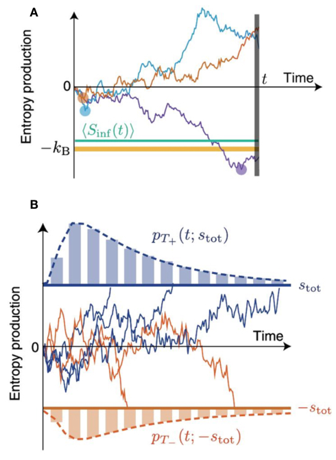
From a thermodynamics perspective, this insight, implies that the average time it takes for a given process to produce a certain amount of entropy, must equal the average time it takes the same process to consume this amount of entropy. The latter process, of course, would be less likely to occur. In a related recent study, Neri et al. Neri et al. (2017) discuss the properties of “stopping times” of entropy production processes using a rigorous mathematical approach. The stopping time here is defined as the time a process on average takes to produce or consume a certain amount of entropy relative to time $t_{0}$. This stopping time equivalence is sketched in Fig. 6B. Importantly, stopping times are first passage times conditioned on the process actually reaching the threshold. The distribution of stopping times, therefore does not say anything about how probable it is for an observer to witness the process of reaching the threshold at all. Only if a trajectory reaches the threshold, the conditional first passage time can be measured. Fig. 6A depicts another property of the entropy $S(t)$: the average entropy is bounded from below by $k_{B}$.

Figure 6: Entropy as a stochastic variable: Illustration of the mean infimum inequality and the equivalence of entropy production stopping times. A) The minimum of the average of an ensemble of entropy-trajectories (purple, red and blue) $\langle S_{\text{inf}}(t)\rangle$ (cyan) is bound from below by $k_{B}$ (thick yellow). B) For entropy-bounds $\pm s_{\text{tot}}$ that are symmetrically placed around $0$ (thick red and blue), the stopping times $T_{+}$ and $T_{-}$ share the same probability distribution (the figure shows unnormalized histograms). The stopping time $T_{+}$ ($T_{-}$) here is defined as the first-passage time of the entropy past the upper (lower) bound. Adapted from Neri et al. (2017)

These ideas were further illustrated by a few examples. The time a discrete molecular stepper, similar to the one illustrated in Fig. 9, would spend making $N$ steps forward in a row, on average, is the same as it would spent making $N$ steps backwards. This results from the way the entropy production for this system scales with the position, $S_{\text{tot}}(t)=-N(t)Fl/(k_{B}T)$, where $F$ is the driving force and $l$ denotes the step length. Related first-passage-time equivalences have been discussed in the context of transport Berezhkovskii et al. (2006), enzymes Qian and Sunney Xie (2006), molecular motors Kolomeisky et al. (2005), and drift-diffusion processes Stern (1977). Entropy stopping times, however, provide a unifying and fruitful perspective on first passage times of thermodynamic processes.

Living systems form one of the most intriguing candidates to apply key concepts of stochastic thermodynamic. Several fluctuation relations have been experimentally verified for various biological processes Loutchko et al. (2017); Berg (2008); Liphardt (2002) and a stochastic thermodynamic description for chemical reaction networks have been developed Schmiedl and Seifert (2007b) and applied, for instance, in catalytic enzymatic cycles Loutchko et al. (2017). A multitude of thermodynamic equalities and lower bound inequalities involving the entropy production have been used to investigate the efficiency of biological systems. This provides insight into the energy dissipation required for a system to perform its biological function at some degree of accuracy. Important contributions in this direction can be found, for instance, in Schmiedl and Seifert (2008) where the efficiency of molecular motors in transforming ATP-derived chemical energy into mechanical work is discussed. Following this line, we could ask how precise cells can sense their environment and use this information for their internal regulation. This was addressed in several works Hartich et al. (2015); Lan et al. (2012); Mehta and Schwab (2012), highlighting a close connection between the amount of entropy produced by the cellular reaction network responsible for performing the “measurement”, and the accuracy of the final measured information (See III.2). In England (2013, 2015) these concepts were further expanded and applied to more complex macroscopic systems, such as the self-replication of bacteria, whose description is not captured by a simple system of chemical reaction networks. Despite the system’s complexity, insightful results were obtained by deriving the more general inequality:

$$\beta\langle\Delta Q\rangle_{I\rightarrow II}+\Delta S_{int}\geq-\ln\frac{\pi(II\rightarrow I)}{\pi(I\rightarrow II)}$$ (15)

where the system’s irreversibility, i.e the ratio between the probability of transition between two macrostates $\pi(II\rightarrow I)$ and its reverse, represents a lower bound for the total entropy production $\beta\langle\Delta Q\rangle_{I\rightarrow II}+\Delta S_{int}$, $\beta=1/k_{\rm B}T$, and $\Delta Q$ is the heat dissipated in the environment. One can now identify the two macrostates $I$ and $II$ with an environment containing one and two bacterial cells respectively. Using probabilistic arguments it is then possible to express the probability ratio in Eq. (15) as a function of measurable parameters, which characterize the system’s dynamics. With this approach, one can make a quantitative comparison between the actual heat produced by E.coli bacteria during a self-replication event and the physical lower bound imposed by thermodynamics constraints. These results may also have implications for the adaptation of internally driven systems, which are discussed inEngland (2015); Perunov et al. (2016).

III.1 Coordinate invariance in multivariate stochastic systems

Energy dissipation, variability, unpredictability are traits not exclusively found in biological systems. In fact, it was a meterologist, Edward Lorenz, who coined the term ’butterfly effect’ to describe an unusually high sensitivity on initial conditions in what are now known as ’chaotic systems’  Rouvas-Nicolis and Nicolis (2009). In a fresh attempt to explain their large variability, stochastic models have been applied to periodically recurring meteorological systems. El-Ni$\tilde{\rm n}$o, for example, is characterized by a slow oscillation of the sea surface temperature, which can cause violent weather patterns when the temperature is close to its maximum. Such a change in temperature can lead to new steady-states, in which the system is permanently driven out-of equilibrium under constant dissipation of energy and exhibits a rich diversity of weather ’states’. Out of equilibrium, transitions between states are still random, but certain transitions clearly unfold in a preferred temporal sequence.

Interestingly, in an effort to model meteorological systems stochastically, Weiss uncovered a direct link between energy dissipation and variability, which is intimately related to broken detailed balance Weiss (2003). More specifically, he found that out-of equilibrium systems can react more violently to perturbations than their more well-behaved equilibrium counterparts. This finding may be relevant in a much broader context, including biology, and we will therefore briefly summarize the main points here. Specifically, we will briefly explore this phenomenon of noise amplification from a perspective of coordinate-invariant properties Weiss (2003).

In an open thermodynamic system in equilibrium, all state variables $\vec{x}$, are subject to the dialectic interplay of random forcing (noise) $\vec{\xi}$, relaxation, and dissipation. Consider an overdamped two-bead toy system at equilibrium, for example (see Fig. 12A and Sec. IV.2.3), where the two beads are coupled by springs and are placed in contact with independent heat baths. Energy stored in the springs is permanently released and refuelled by the thermal bath, and flows back and forth between the two colloids in a balanced way. A sustained difference in temperature between the beads, $T_{1}\neq T_{2}$, however, will permanently rectify the flow of energy and break this balance. Crucially, this temperature difference is a matter of perspective. If we set, for example, $T_{1}=0$, then bead $1$ will not receive any noise any more and energy will flow to it from bead number $2$. Interestingly, if we look at the normal coordinates of the beads $u_{1}(t)=(x_{1}(t)-x_{2}(t))/2$ and $u_{2}(t)=(x_{1}(t)+x_{2}(t))/2$, we find that their respective thermal noise has exactly the same temperature $T_{2}/2$. However, if we could measure the fluctuations of noise in these coordinates, we would find that both noise terms correlate. Thus, in this case, mode $1$ and $2$ are driven not only by the same temperature, but by the very same white noise process.

Correlations amongst noise processes $\xi_{1}(t)$ and $\xi_{2}(t)$ exciting different variables $x_{1}(t)$ and $x_{2}(t)$ can, in principle, break detailed balance, even if the overall variance of the noise is equal in all directions, i.e. $\langle\xi_{1}^{2}\rangle=\langle\xi^{2}_{2}\rangle$. In other words, correlations in random forces in one coordinate system, result in differences in temperature in other coordinates and vice-versa. The simple temperature criterion $T_{1}=T_{2}$ is thus insufficient to rule out broken detailed balance (see Section IV.1); a comprehensive coordinate-invariant criterion is required.

Consider variables $\vec{x}(t)$ of a generic system, evolving stochastically according to a Langevin equation (16),

$$\frac{\mathrm{d}\vec{x}}{\mathrm{d}t}(t) =\mathbf{A}\vec{x}(t)+\mathbf{F}\vec{\xi}(t)$$ (16)

while the dynamics of the associated probability density $\rho(\vec{x},t)$ is given by the corresponding Fokker-Planck equation (17).

$$\frac{\partial\rho}{\partial t}\left(\vec{x},t\right) =-\nabla\cdot\left(\mathbf{A}\vec{x}\rho\left(\vec{x},t\right)-\mathbf{D}\nabla\rho\left(\vec{x},t\right)\right)$$ (17)

In the equations above, $\mathbf{F}$ denotes the forcing matrix, in which any noise variance is absorbed, such that $\vec{\xi}$ here has unit variance $\langle\vec{\xi}(t)\vec{\xi}^{T}(t^{\prime})\rangle=\mathbf{1}\delta(t-t^{\prime})$. The forcing matrix is directly related to the diffusion matrix $\mathbf{D}=\frac{1}{2}\mathbf{F}^{T}\mathbf{F}$, and the term $\mathbf{A}\vec{x}$ describes deterministic forces, and the matrix $\mathbf{A}$ therefore contains all relaxational timescales. Any linear system with additive, state-independent white noise $\vec{\xi}$ can be mapped onto these generic equations.

In an equilibrium system with independent noise processes, $\mathbf{D}$ is diagonal and fulfills the standard fluctuation-dissipation theorem $\mathbf{D}=\frac{k_{B}T}{\gamma}\mathbf{1}$, where $\gamma$ denotes the friction coefficient. In steady-state, the correlation matrix $\mathbf{C}=\langle\vec{x}\cdot\vec{x}^{T}\rangle$ in and out of equilibrium obeys the Lyanpunov equation $\mathbf{A}\mathbf{C}+\mathbf{C}\mathbf{A}^{T}=-2\mathbf{D}$, which can be thought of as a multidimensional FDT. The density $\rho$ can therefore always be written as a multivariate Gaussian distribution $\rho(\vec{x},t)=1/\sqrt{|\mathbf{C}|}e^{-\frac{1}{2}\vec{x}^{T}\mathbf{C}^{-1}\vec{x}}$.

Apart from systems with temperature gradients, detailed balance is also broken in systems with non-conservative forces $\mathbf{A}\vec{x}$, which have a non-zero rotation $\partial_{i}\left(\mathbf{A}\vec{x}\right)_{j}\neq\partial_{j}\left(\mathbf{A}\vec{x}\right)_{i}$. Within our matrix framework, this condition simplifies to $A_{i,j}\neq A_{j,i}$ and thus requires $\mathbf{A}$ to be symmetric in equilibrium. For instance, if we consider the two bead model in Sec. IV.2.3, $\mathbf{A}$ would represent a product between a mobility matrix and a stiffness matrix, both of which are symmetric resulting in a symmetric $\mathbf{A}$. Note, this framework only applies to systems with dissipative coupling; reactive currents require a separate analysis. The two ways of breaking detailed balance in our case (temperature gradients and non-conservative forces) are reflected by a coordinate-independent commutation criterion for equilibrium Weiss (2003):

$$\mathbf{A}\mathbf{D}-\mathbf{D}\mathbf{A}^{T}=0.$$ (18)

It was also argued that a system with broken detailed balance will sustain a larger variance than a similar system with the same level of noise, which is in equilibrium. This effect, referred to by Weiss as noise amplification, had previously been attributed to non-normality of the matrix $\mathbf{A}$, which is only true for diagonal $\mathbf{D}$. This type of noise amplification is now understood to be caused by broken detailed balance.

Although this amplification can be captured by different metrics, we here focus on the gain matrix $\mathbf{G}=\mathbf{1}+\mathbf{A}\mathbf{C}\mathbf{D}^{-1}$. The gain matrix is a measure of the variance of the system normalized by the amplitude of the noise input. To obtain a scalar measure, one can take, for example, the determinant of $\mathbf{G}$ which yields the gain $g$. It can be shown, that $g\geq g_{0}$ when detailed balance is broken, where $g_{0}$ is the gain of the same system in equilibrium. Finally, it is interesting to note, that the noise amplification matrix $\mathbf{G}$ is related to the average production of entropy in our generic model system. Let $\Pi$ denote the production of entropy, then

$$\Pi =k_{B}\rm{tr}\left(\mathbf{A}\mathbf{G}\right),$$ (19)

providing a direct link between dissipation and increased variability in multivariate systems out of equilibrium.

III.2 Energy-speed-accuracy trade-off in sensory adaption

Energy dissipation is essential to various control circuits found in living organisms. Faced with the noise inherent to small systems, cells are believed to have evolved strategies to increase the accuracy, efficiency, and robustness of their chemical reaction networks Barkai and Leibler (1997); Alon et al. (1999); Qian (2006). Implementing these strategies, however, comes at an energetic price, as is exemplified by Lan et al. in the case of the energy-speed-accuracy (ESA) trade-off in sensory adaption Lan et al. (2012). This particular circuit is, of course, not the only active control in cell biology. The canonical example of molecular ‘quality control’ is the kinetic proofreading process, in which chemical energy is used to ensure low error rates in gene transcription and translation Hopfield (1974). Furthermore, fast and accurate learning and inference processes, which form the basis of sensing and adaptation, require some energy due to the inherent cost of information processing Mehta and Schwab (2012); Ito and Sagawa (2013); Sartori et al. (2014); Lang et al. (2014).

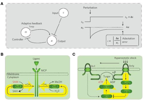
Sensory learning and adaptation at the cellular level involves chemical feedback circuits that are directly or indirectly driven by ATP hydrolysis, which provides energy input to break detailed balance. Examples of adaptation circuits are shown schematically in Fig. 7B,C. These examples include the chemotactic adaption mechanism in E. coli (panel (B)), a well-established model system for environmental sensing. Common to all circuits is a three-node feedback structure, as depicted in Fig. 7A. Conceptually, this negative feedback circuit aims to sustain a given level of activity $a_{0}$, independent of the steady amplitude of an external stimulus $s$, which here is assumed to be inhibitory. This adaptive behavior allows the circuit to respond sensitively to changes to the external stimulus over a large dynamic range in $s$.

Figure 7: Models of adaptive feedback systems. A) Simplified topology of a feedback circuit. The input $s$ here is chosen to have an inhibitory effect. On the right the response of the output $a$ is shown following a step in the input $s$. B) Chemotactic circuit in E. coli. Ligand binding to a methyl-accepting-protein (MCP) causes further addition (mediated by CheR) or deletion (mediated by CheB) of methylgroups to MCP. This methylation counteracts the effects of ligand binding. C) Osmotic sensing circuit in yeast. A reduction of osmolarity results in dephosphorylation of Sln1p$\to$ Sln1, which activates the HOG1 (High osmolarity glycerol) mechanism. This mechanism acts to restore the tugor pressure inside the cell and eventually phosphorylates Sln1$\to$Sln1p. Adapted from Lan et al Lan et al. (2012).

The authors condense the dynamics of such a chemical network into a simple model (Fig. 7A) with abstract control $m(t)$ and activity $a(t)$ variables described by two coupled Langevin equations,

$$\dot{a} =F_{a}(a,m,s)+\xi_{a}(t)$$ (20)

$$\dot{m} =F_{m}(a,m,s)+\xi_{m}(t)$$ (21)

with $F_{a}$, $F_{m}$ denoting the coarse-grained biochemical response and $\xi_{a}$, $\xi_{m}$ being white-noise processes with different variances $2\Delta_{a}$ and $2\Delta_{m}$, respectively. Importantly, these biochemical responses do not fulfil the condition for conservative forces discussed in the previous section (above Eq. (18)). To function as an adaptive system with negative feedback, $\partial_{m}F_{a}$ and $\partial_{a}F_{m}$ must have different signs, which implies a breaking of detailed balance. Indeed, adaptation manifests in a sustained probability current $J=(J_{a},J_{m})$ in the phase space spanned by $a\times m$; the energetic cost to maintain this non-equilibrium steady-state is given by the amount of heat exchanged with the environment per unit time, which must equal the entropy production rate $\Pi$ multiplied by the temperature $T$ of the heatbath to which the system is coupled.

In general, a non-equilibrium system at steady-state that adheres to a Fokker-Planck equation produces entropy at a rate Tomé and de Oliveira (2012); Seifert (2012),

$$\Pi =k_{B}\int\,\mathrm{d}\vec{x}\sum\limits_{i}\frac{J_{i}(\vec{x},t)^{2}}{D_{i}\rho(\vec{x},t)}.$$ (22)

where $\rho(\vec{x},t)$ is the probability density in phase space, $D_{i}$ is the diffusion coefficient, and the sum runs over all phase space variables. Applying Eq. (22) to the model above for sensory adaption, yields the heat exchange rate $\dot{W}\leavevmode\nobreak\ =\leavevmode\nobreak\ \int\leavevmode\nobreak\ \int\leavevmode\nobreak\ \mathrm{d}m\mathrm{d}a\left[J_{a}^{2}/(\Delta_{a}\rho)\leavevmode\nobreak\ +\leavevmode\nobreak\ J_{m}^{2}/(\Delta_{m}\rho)\right]$. An assumed separation of timescales that govern the fast activity $a$ and the slower control $m$, allows the authors to derive an Energy-Speed-Accuracy (ESA) relation, which reads

$$\dot{W} \approx(c_{0}\sigma_{a}^{2})\omega_{m}\log\left(\frac{\epsilon_{0}}{\epsilon}\right),$$ (23)

where, $\sigma_{a}^{2}$ represents the variance of the activity, and $\epsilon$ denotes the adaptation error defined as $\epsilon\equiv\left|1-\langle a\rangle/a_{0}\right|$, while $c_{0}$ and $\epsilon_{0}$ are constants that depend on details of the model. Here, $\omega_{m}$ parametrizes the rate of the control variable $m$. Therefore, an increase in $\omega_{m}$ or a reduction in $\epsilon$ requires an increased dissipation $\dot{W}$; put simply, swift and accurate adaptation can only be achieved at high energetic cost.

Figure 8: Experimental evidence for an energy-speed-accuracy (ESA) trade-off in E. coli chemotaxis. A) Ratio of intensity of fluorescent reporters of adaptation. Changes in this signal are indicative of adaptation in the chemotatic circuit to external stimuli presented by the addition/removal of MeAsp. The inset illustrates the reduction of the FRET signal at the three different points in time indicated by arrows. B) Half-times inferred from the responses to addition/removal cycles shown in A). C) Relative accuracies of adaptation. Adapted from Lan et al. (2012).

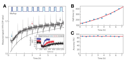
The authors argue that a dilution of chemical energy in living bacteria will mainly affect the adaptation rate, but leave the adaptation error unchanged. Starvation should therefore lead to lower adaptation rates to uphold the ESA relation. This prediction was tested in starving E. coli colonies under repeated addition and removal of MeAsp (see Fig. 8), an attractant which stimulates the chemotactic system shown in Fig. 7B. The cells in this study were engineered to express fluorescent markers attached to two proteins involved in adaptation. Physical proximity between any of these two molecules is an indicator of ongoing chemosensing, and was measured using Foerster-resonance-energy transfer (FRET). Since the donor-acceptor distance correlates with the acceptor intensity, but anticorrelates with the donor intensity, the ratio of YFP (acceptor) and CFP (donor) intensities lends itself as a readout signal to monitor adaptation. Indeed, after each addition/removal cycle of MeAsp, the signal recovers, albeit at a gradually decreasing pace, as is shown in the inset in Fig. 8A. The decrease in the speed of adaptation is attributed to the progressing depletion of nutrition in the colony. In panels b and c, the adaptation half-time and relative accuracy are plotted. The graph in panel c clearly demonstrates the constancy of the accuracy of chemotatic system as nutrients are depleted over time, which is argued to be close to optimality.

III.3 Current fluctuations in non-equilibrium systems

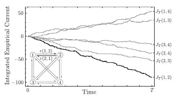
Directed and chemically-specific transport of proteins, RNA, ions, and other molecules across the various membranes that foliate the cell is often achieved by active processes. A library of active membrane channel proteins has been described, which ‘pump’ ions into and out of cells to control osmolarity, the electrical potential or the pH Stein and Litman (2014). Furthermore, in eukaryotic cells, a concentration gradient of signalling molecules across the nuclear envelope causes messenger RNA (mRNA) molecules, expressed within the nucleus, to diffuse outwards through channels known as nuclear pore complexes (NPC) Alberts et al. (1994). Outside of the nucleus, the mRNA is translated into proteins by the ribosomes, which are too large to traverse the NPCs. All these directed transport processes are essential to the cell. Thus, this raises the question of reliability of such processes Bezrukov et al. (2000); Berezhkovskii and Bezrukov (2008). For example, how steady should we expect the supply of mRNA to the ribosomes to be Grünwald et al. (2011)? Or, more generally, how predictable is the output rate of any given non-equilibrium process? Even active processes still endure fluctuations: molecular motors, at times, make a step backwards, or stall. Polymerizing filaments will undergo brief periods of sluggish growth or even shrinkage. Similarly, active membrane channels will sometimes transport more, and in other times fewer molecules. To illustrate this, an abstract example of such current fluctuations is depicted in Fig. 10, which will be further discussed below.

Figure 9: Variability of non-equilibrium steady states: A) Example trajectories to show the spread in the average position $\langle x(t)\rangle$ after $t$ steps. The inset depicts a simple model for a molecular motor in a sawtooth potential. B) The products $TS(t)\epsilon(t)^{2}$ calculated over an ensemble of trajectories are bounded from below by the uncertainty relation. Despite the small size of the ensemble (100), Eq. (24) is fulfilled.

Figure 10: Variability of non-equilibrium steady states: Fluctuations of the cumulative probability current $J_{T}(m,n)=\int^{T}j_{m,n}(t)\mathrm{d}t$ along all nodes in the four state system shown in the inset. Fluctuations result in perturbations of the currents around their intrinsic rates $r(m,n)$. Adapted from Gingrich et al. (2016).

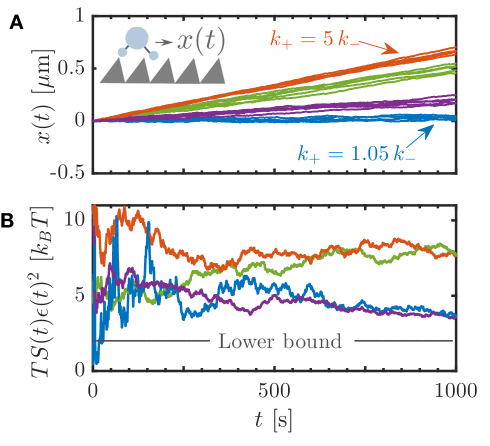
It seems intuitive, that predictability on the microscale always comes with an energy-price tag. In recent years, significant progress has been made to calculate the level of deviations from the average rate of a non-equilibrium process that is to be expected over finite times Barato and Seifert (2015); Machta (2015); Gingrich et al. (2016); Pietzonka et al. (2016, 2017); Horowitz and Gingrich (2017). More formally, a universal bound for finite-time fluctuations of a probability current in steady-state has been established. Such an uncertainty relation is perhaps best illustrated by the simple motor model discussed by Barato et al. Barato and Seifert (2015): A molecular motor moves to the right at a rate $k_{+}$, and to the left at a rate $k_{-}$. The movement is biased, i.e. $k_{+}>k_{-}$, driven by a free energy gradient $\Delta\mathcal{F}=k_{B}T\log\left(k_{+}/k_{-}\right)$. A few trajectories for various values of $k_{+}$ are depicted in Fig. 9A. As can be seen, the walker (shown in the inset), on average, moves with a constant drift $\langle x(t)\rangle=t(k_{+}-k_{-})$. Associated with this drift is a constant rate of entropy production $\Pi=(k_{+}-k_{-})\Delta\mathcal{F}/T$. Barato et al. showed that the product of the total entropy produced $S(t)=\Pi t$ and the squared uncertainty $\epsilon^{2}=\langle(x(t)-\langle x(t)\rangle)^{2}\rangle/\langle x(t)\rangle^{2}$ always fulfils the bound

$$TS(t)\epsilon(t)^{2}\geq 2k_{B}T.$$ (24)

For this particular model, the square uncertainty reads $\epsilon(t)^{2}=(k_{+}+k_{-})/[(k_{+}-k_{-})t]$, such that the product $TS(t)\epsilon(t)^{2}$ is constant in time. To further illustrate this point, we plotted the quantity $TS(t)\epsilon(t)^{2}$ for each choice of $k_{+}$ in Fig. 9A, averaged over an ensemble of a hundred simulated trajectories in Fig. 9B. Due to the finite ensemble size, the graphs fluctuate, but stay well above the universal lower bound of $2k_{B}T$ for longer times $t$. So far, the theory underlying uncertainty relations was shown to be valid in the long time limit. Only recently, its validity has been extended to finite time scales Pietzonka et al. (2017); Horowitz and Gingrich (2017).

The bound in Eq. (24) can be generalized to any non-equilibrium steady-state Gingrich et al. (2016); Pietzonka et al. (2016). For a Markov system, such as the four-node system in the inset in Fig. 10, the integrated current $J_{t}=\int^{t}j(t^{\prime})\mathrm{d}t^{\prime}$ between any two nodes is distributed as $P(J_{t}=tj)\sim e^{-tI(j)}$, with $I(j)$ denoting the large deviation function. This function therefore controls the variability of $J_{t}$. Interestingly, it can be shown that the large deviation function obtained in the linear response regime $I_{\text{LR}}$, is never exceeded by $I$, even far away from equilibrium Gingrich et al. (2016). Thus, an increase in currents is accompanied by an increase in the variability of these currents when a system is driven further away from equilibrium.

This general lower bound for the squared uncertainty $\epsilon^{2}$ is shown to be given by $2/\Sigma$, i.e. $\epsilon^{2}\geq 2/\Sigma$, where $\Sigma\leavevmode\nobreak\ =\leavevmode\nobreak\ \sum_{m<n}j(m,n)\log[(\rho(m)r(m,n))/(\rho(n)r(n,m))]$ is the average dissipation rate in the system in steady-state. The steady-state probability distribution is denoted here by $\rho(m)$. The relation above is a bound for the uncertainty of the entire system. A similar relation also applies to any individual edge between two nodes $n$ and $m$, $\langle(j(m,n)-\langle j(m,n)\rangle)^{2}\rangle/\langle j(m,n)\rangle^{2}\geq 2/\Pi(m,n)$, where $\Pi(m,n)$ denotes the entropy production associated with the edge $(m,n)$.

While the uncertainty relations discussed above appear abstract at first, they may soon prove useful in studying transport or control systems in cellular biology due to their general applicability. Reminiscent of Carnot’s efficiency for macroscopic engines, one implication of Eq. (24) is that a reduction in uncertainty can only be achieved by dissipating more energy when the system is close to optimality.

IV Detecting broken detailed balance in living systems

Up to this point we discussed intrinsically invasive methods to probe biological systems for non-equilibrium dynamics. For instance, to determine violations of the fluctuation-dissipation theorem a response function is required, which can only be measured by performing a perturbation in non-equilibrium systems (see Section II). Other methods that are used to probe for non-equilibrium involve thermal or chemical perturbations, and are therefore also inherently invasive. Such approaches are not ideal for investigating the stochastic dynamics of delicate sub-cellular system. Performing a controlled perturbation of such a system might not only be technically challenging, it may also be undesirable because of potential effects on the behavior or function of such a fragile system.

Ideally, we would like to avoid the technical and conceptual difficulties of invasive protocols to probe for non-equilibrium behavior. This raises the question: Could we perhaps measure a system’s non-equilibrium behavior simply by looking at it? With this purpose in mind, we recently developed a method that indeed uses conventional video microscopy data of cellular and subcellular systems Battle et al. (2016). Detecting non-equilibrium behavior in the stochastic dynamics of mesoscopic coordinates of such systems can be accomplished by demonstrating that these dynamics break detailed balance. In this section, we will illustrate these ideas and discuss some recent related theoretical developments.

IV.1 Equilibrium, steady state, and detailed balance

Suppose we can describe a system on a mesoscopic level by dividing phase space into small cells, such that the state of the system can be described by a state variable $n$. If the system is ergodic and irreducible, it will evolve towards a unique stationary solution $p_{n}^{(s)}$, which is constant in time. A necessary and sufficient requirement for such steady-state conditions is that the rate of transitions into any particular microstate, $m$, is balanced by the total rate of transitions from $m$ to other microstates $n$:

$$\sum_{n}W_{n,m}=\sum_{n}W_{m,n},$$ (25)

where $W_{n,m}$ describes the rate of transitions from state $m$ to $n$. This result must hold for any system, at equilibrium or far from equilibrium, that has reached steady state conditions. When the system is Markovian, Eq.(25) reduces to

$$\sum_{n}w_{nm}p_{m}^{(s)}=\sum_{n}w_{mn}p_{n}^{(s)},$$ (26)

where $w_{nm}$ describes the rate of transitions from state $m$ to $n$, given that the system is in state $m$.

In thermodynamics equilibrium, it can be shown that a system must obey an even stronger condition: detailed balance. Classical closed ergodic systems are characterized by a time-independent Hamiltonian, which we will here restrict to be an even function of the momenta and independent of magnetic fields. The microscopic degrees of freedom of such a system obey deterministic dynamics described by Hamilton’s equations, which are time reversal invariant. This has important implications also for the probability distribution of mesoscopic observables, which characterize the systems states at thermodynamic equilibrium. Consider, for instance, a mesoscopic variable $y$, which represents a generalized coordinate that either does not depend on the microscopic momenta, or that is an even functions of the microscopic momenta. Then, the transition between states must obey Gardiner (1985)

$$p_{2}^{(e)}(y_{2},\tau;y_{1},0)=p_{2}^{(e)}(y_{1},\tau;y_{2},0)\,.$$ (27)

Here we indicate with $p_{2}^{(e)}$ the two-point joint probability distribution. This result is referred to as the principle of detailed balance. Put simply, it means that the transitions between any two mesostates are pairwise balanced, and this result derives from the transition rates between any two microstates are also being pairwise balanced. For Markovian systems we can write detailed balance more conveniently as

$$w(y_{2}|y_{1})p^{(e)}(y_{1})=w(y_{1}|y_{2})p^{(e)}(y_{2})\,,$$ (28)

where the $w$’s indicate the conditional rates between states. Finally, we note that if we add observables $z$, which are odd functions of the momenta, Eq. 27 needs to be generalized to

$$p_{2}^{(e)}(y_{2},z_{2},\tau;y_{1},z_{1},0)=p_{2}^{(e)}(y_{1},-z_{1},\tau;y_{2},-z_{2},0)\,.$$ (29)

It is important to note that for a system in steady state dynamics, broken detailed balance is direct evidence of non-equilibrium, but showing that a system obeys detailed balance in a subspace of coordinates is insufficient to prove equilibrium. Indeed, even for systems out of equilibrium, broken detailed balance is not necessarily apparent at the supramolecular scale Egolf (2000); Rupprecht and Prost (2016); Gladrow et al. (2016, 2017). One can also often observe stationary stochastic processes in cells that, at first glance, appear to be thermally driven. Examples include the fluctuations of cytoskeletal filaments such as microtubuli, F-actin filaments or the fluctuations of intracellular organelles. These cases should be contrasted with obvious examples of mesoscopic non-equilibrium, non-stationary, irreversible processes such as cell growth, locomotion and mitosis. Thus, in general, it is unclear how and when broken detailed balance that realized on the molecular level also manifests at larger scales.

IV.2 Probability Flux Analysis

In this section, we describe the basis and methodology that can be used to infer broken detailed balance from microscopy data. We consider a system, which is assumed to evolve according to stationary dynamics. This could, for instance, be a primary cilium or a flagellum Battle et al. (2016). In general, these system exhibits stochastic dynamics, comprised of both a deterministic and a stochastic component. The dynamics of such a system can be captured by conventional video microscopy. To quantify this measured stochastic dynamics, we first need to parameterize the configuration of the system. The shape of a flagellum, for instance, could be conveniently decomposed into the dynamic normal modes of an elastic beam. In this example, the corresponding mode amplitudes represent time-dependent generalized coordinates of the system. Note, these mode amplitudes can be extracted from a single time frame and strictly represent configurational coordinates, which are independent of the microscopic momenta.

In general, a video microsocopy experiment can be used to extract time traces of $D$ mesoscopic tracked coordinates $x_{1},...,x_{D}$, which represent the instantaneous configuration of the system. Clearly, this only represents a chosen subset of all coordinates that completely specify the whole system. Furthermore, only spatial or conformational degrees of freedom are considered in this discussion here. Indeed, fluctuations in momenta in a typical overdamped biological or soft-matter systems relax on very short time-scales, which are not resolved in typical video microscopy experiments. However, the basic methodology described below can readily be generalized to also include momentum-like variables.

We define a probability density, $\rho(x_{1},...,x_{D},t)$, in terms of only the tracked degrees of freedom. This probability density can be obtained from the full joint probability density in terms of a complete set of variables, by integrating out all the untracked degrees of freedom. In the reduced configurational phase space of the tracked degrees of freedom, the dynamics of the system still obeys a continuity equation:

$$\frac{\partial\rho(x_{1},...,x_{D},t)}{\partial t}=-\nabla\cdot\vec{j}(x_{1},...,x_{D},t)$$ (30)

where $\vec{j}(x_{1},...,x_{D},t)$ is the current density describing the net flow of transitions of the system in the D-dimensional configurational phase space. Here, we only consider systems with dissipative currents Chaikin and Lubensky (1995). While at steady state the divergence of the current needs to vanish, in equilibrium any dissipative current itself must be identically zero.

IV.2.1 Estimating phase space currents

Here we discuss one way of estimating currents from a set of time-traces. To provide a simple illustration of this approach, we consider a system with a two-dimensional configurational phase space, as illustrated in Fig. 11A. The dynamics of the system is captured by a time trace in this configurational phase space. It is convenient to analyze these trajectories using a discretized coarse-grained representation of the two-dimensional phase space. This Coarse-Grained Phase Space (CGPS) consists of a collection of equally sized, rectangular boxes, each of which represents a discrete state Fig. 11B. Such a discrete state in CGPS encompasses a continuous set of microstates, each of which belongs to a unique, discrete state. The primary reason for using this discretized representation of phase space is to be able to obtain informative results on experimental data with limited statistics.

In this two-dimensional CGPS, a discrete state $\alpha$ has two neighboring states, respectively $\alpha_{+}$ (larger $x_{i}$) and $\alpha_{-}$ (smaller $x_{i}$), along each direction $x_{i}$, resulting in four possible transitions. The dynamics of the system indeed satisfies the continuity equation

$$\frac{dp_{\alpha}}{dt}=-\tilde{W}_{\alpha^{-},\alpha}^{(x_{1})}+\tilde{W}_{\alpha,\alpha^{+}}^{(x_{1})}-\tilde{W}_{\alpha^{-},\alpha}^{(x_{2})}+\tilde{W}_{\alpha,\alpha^{+}}^{(x_{2})},$$ (31)

where $\tilde{W}_{\alpha,\beta}=W_{\alpha,\beta}-W_{\beta,\alpha}$ is the net rate of transitions from state $\beta$ to $\alpha$ and $p_{\alpha}$ is the probability to be in discrete state $\alpha$, which will become time independent when the system reaches steady-state conditions.

This probability $p_{\alpha}$ is related to the probability density $\rho(x_{1},...,x_{2},t)$ defined above, and can be obtained by integrating $\rho$ over the volume of state $\alpha$ in CGPS. We can estimate this probability from a measured trajectory by using

$$p_{\alpha}=t_{\alpha}/t_{\rm total},$$ (32)

where $t_{\alpha}$ is the accumulated time that the system spends in state $\alpha$ and $t_{\rm total}$ is the total duration of the experiment.

The net rates $\tilde{W}$ in CGPS can be estimated from the measured trajectories simply by counting the net number of transitions per unit time:

$$\tilde{W}_{\alpha,\beta}^{(x_{i})}=\frac{N_{\alpha,\beta}^{(x_{i})}-N_{\beta,\alpha}^{(x_{i})}}{t_{\rm total}}$$ (33)

Here $N_{\alpha,\beta}^{(x_{i})}$ is the number of transitions from state $\beta$ to state $\alpha$ along the direction $x_{i}$. In a mechanical system, the trajectories through phase space are continuous such that there can be only transitions between neighboring states. However, due to the discreteness in a measured time trajectory, it is possible that a transition between neighboring states is “skipped”, resulting in an apparent transition between non-neighboring states. In these cases, it is convenient to perform an interpolation of the time trace to estimate the intermediate transitions. It is important that this interpolation is performed in a time-symmetric way, so that the interpolation filter preserves time-reversal symmetry. In fact, this should be taken into account with any kind of filtering that is performed on measured time traces.

The currents in CGPS that describes back-and-forth transitions through all four boundaries of the box associated with a discrete state (Fig. 11C), can be defined by:

$$\vec{j}(\vec{x}_{\alpha})=\frac{1}{2}\left(\tilde{W}_{\alpha^{-},\alpha}^{(x_{1})}+\tilde{W}_{\alpha,\alpha^{+}}^{(x_{1})},\tilde{W}_{\alpha^{-},\alpha}^{(x_{2})}+\tilde{W}_{\alpha,\alpha^{+}}^{(x_{2})}\right).$$ (34)

Here, $\vec{x}_{\alpha}$ is the center position of the box associated with state $\alpha$.

With this approach, prominent examples such as an isolated beating flagella of Chlamydomonas reinhardtii were examined Battle et al. (2016) (see Fig. 1). Dynein motors drive relative axial sliding of microtubules inside the axoneme of the flagellum  Ma et al. (2014); Riedel?Kruse et al. (2007); Wan and Goldstein (2014). To quantify the non-equilibrium dynamics of this system, we decomposed the axoneme shapes measured using time-lapse microscopy into the dynamic normal modes of an elastic filament freely suspended in a liquid. Using this approach, we obtained the amplitudes of the projections coefficients for the first 3 modes. These amplitude time series were used to construct a trajectory in a phase space spanned by the three lowest-order modes, which were analyzed using PFA, as shown in Fig. 1C. Here, the vector fields indicate the fluxes for the first three modes. Thus, this method can be used to quantify the non-equilibrium dynamics of the flagellum in a phase space of configurational degrees of freedom.

In addition, we considered primary cilia of Madin-Darby Canine Kidney (MDCK II) epithelial. Primary cilia are hair-like mechano and chemosensive organelles that grow from the periphery of certain eukaryotic cells Singla (2006); Battle et al. (2015); Barnes (1961). At first glance the dynamics of the deflection angle and curvature of primary cilia appear to exhibit random fluctuations. Using Probability Flux Analysis (PFA), however, it was demonstrated that there are significant circulating probability fluxes in a configurational phase space of angle and curvature, providing evidence for the non-equilibrium nature of primary cilia Battle et al. (2016). This approach is now gaining traction in variety of systems, ranging from the post translation Kai circadian clock  Paijmans et al. (2017) to motility phenotypes J. C. Kimmel et al. (2017). When the mobility of a system is known, a related approach can be used to estimate the heat dissipation Lander et al. (2012). However, in a non-equilibrium system, the mobility must be obtained by a perturbative measurement.

Figure 11: Schematic illustrating the coarse-graining procedure for the estimation of phase space current and corresponding errorbars. A) Trajectory in continuous phase space. B) Grid illustrating the discretization of the continuous phase space. C) By counting transitions between first neighbour discrete states it is possible to estimate the currents (indicated by the arrows) across the boundaries. D) Current errorbars representation obtained through the bootstrapping procedure. Adapted from  Battle et al. (2016).

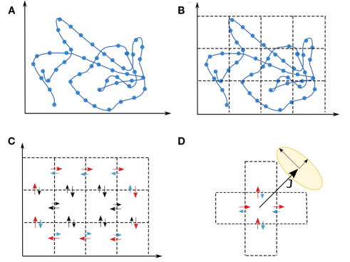
IV.2.2 Bootstrapping

In practice, the finite length of experimental or simulated trajectories limits the accuracy with which we can estimate fluxes in phase space. This has an important implication: even when considering a system at thermodynamic equilibrium, a measurement from finite data will typically result in apparent non-zero currents. In such a case we can not statistically distinguish the measured apparent current from a zero current. Therefore, it is important to asses if the estimated currents are statistically significant. Moreover, these current fluctuations may also be interesting to study in and of themselves (see Section III.3). In this section we briefly describe “bootstrapping”, a method that can be used to associate errorbars to the measured currents.

The error bars on the probability flux can be determined by counting statistics of the number of transitions in Eq.(33). In general, however, there may be correlations between in-and-outward transitions for a given state, which renders it difficult to perform a simple estimate of the errorbar. A possible way around this, which naturally takes correlations into account, is to bootstrap trajectories from the experimentally measured or simulated trajectories.

To perform this bootstrapping procedure, we first determine all the transitions between discrete states in the CGPS from the measured trajectories. From this data, we construct a set $A$ of $n$ events, describing specific transitions of the system between two states, including the transition time. Given $A$, we can generate a new set of transitions, $A^{\prime}$, by randomly sampling $n$ single events (with replacements) from $A$. This procedure, however, ignores possible correlations. To capture the effects of correlations on the accuracy of our current estimator, we bootstrap trajectories by randomly sampling a group of $m$ consecutive events from $A$ to construct a new set of transitions $A^{\prime}_{i}(m)$  Shannon and Weaver (1949).

For each bootstrapped trajectory we calculate the current field and by averaging over all the realizations, we estimate the covariance matrix. To visualize the errorbars (standard error of the mean) on the estimated currents, we depict an ellipse aligned with the principle components of this covariance matrix. The short and long axes of these error-ellipses are defined by the square roots of the small and large eigenvalues, respectively, of the covariance matrix, Fig. 11D. Empirically, we found that the estimated error bars reduce substantially by including pairwise correlations, i.e. in going from $m=1$ to $m=2$, after which the errorbars became largely insensitive to $m$. Such correlations can arise because of the coarse graining of phase space, which can introduce a degree of non-Markovianity.

Figure 12: A) Schematic of the two coupled beads system and simulated time series of the beads positions for $T_{2}=5T_{1}$. B-C)Probability distribution (color) and flux map (white arrows) obtained by Brownian dynamics simulations at equilibrium ($T_{1}=T_{2})$ (B) and non-equilibrium $(T_{2}=5T_{1})$ (C). Translucent discs represent a 2$\sigma$ confidence interval for fluxes. D) Analytical result for the probability distribution (color) and flux map (white arrows) obtained for a non-equilibrium case, ($T_{2}=5T_{1}$). Adapted from Battle et al. (2016) E) Compatibility estimated from Eq.(44) between the estimated and theoretical second components of the currents.

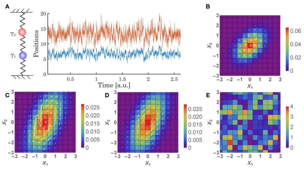
IV.2.3 Toy model: two stochastically driven coupled beads

To provide some basic intuition for stochastic non-equilibrium systems we next discuss a simple model, which can easily be solved both analytically and numerically. With this model, we illustrate how probability flux analysis (PFA) can be used on simulated data to obtain current densities in coarse grained phase space. The results are shown to be consistent with analytical calculations within errorbars.

Consider a system consisting of two microscopic over-damped beads in a liquid connected to each other and to a rigid boundary by springs with elastic constant $k$, as depicted in Fig. 12A. The two beads are assumed to be in contact with two independent heat baths, respectively at temperatures $T_{1}$ and $T_{2}$. The stochastic dynamics of this system is described by the overdamped equation of motion

$$\frac{d\vec{x}}{dt}=\mathbf{A}\vec{x}+\mathbf{F}\vec{\xi},$$ (35)

where $\vec{x}=(x_{1},x_{2})^{T}$ represents the beads positions. The deterministic dynamics is captured by the matrix

$$\mathbf{A}=\frac{k}{\gamma}\begin{pmatrix}-2&1\\ 1&-2\\ \end{pmatrix}.$$ (36)

The drag coefficient $\gamma$, characterizing the viscous interactions between the beads and the liquid, is assumed to be identical for the two beads. The stochastic contribution, $\xi_{i}$, in the equation of motion is defined by

$$\langle\vec{\xi}\rangle=0,\ \ \ \ \ \langle\vec{\xi}(t)\otimes\vec{\xi}(t^{\prime})\rangle=I\delta(t-t^{\prime}),$$ (37)

and the amplitude of the noise is captured by the matrix

$$\mathbf{F}=\sqrt{\frac{2k_{\rm B}}{\gamma}}\begin{pmatrix}\sqrt{T_{1}}&0\\ 0&\sqrt{T_{2}}\end{pmatrix}.$$ (38)

We can generate simulated trajectories for this system by numerically integrating Eq. (35). We will consider two exemplificative cases: i) thermal equilibrium with $T_{1}=T_{2}$, and ii) non-equilibrium with $T_{2}=5T_{1}$. An example of the two simulated trajectories for this last case is shown in Fig. 12A, where we note that the dynamics of individual trajectories appears to be, at first glance, indistinguishable from equilibrium dynamics. Interestingly however, the nonequilibrium nature of this system is revealed by applying PFA to these data, which gives coherently circulating probability fluxes in the phase space (Fig. 12C). By contrast, in the case of thermal equilibrium ($T_{1}=T_{2}$) we find, as expected, that the flux vanishes, as shown in Fig. 12B.

To compare these results of the estimated fluxes from simulations with analytical calculations, we next consider the time evolution for the probability density function $p(\vec{x},t)$ of the system, which is described by the Fokker Planck equation:

$$\frac{\partial p(\vec{x},t)}{\partial t}=-\nabla\cdot[\mathbf{A}\vec{x}p(\vec{x},t)]+\nabla\cdot\mathbf{D}\nabla p(\vec{x},t),$$ (39)

where $\mathbf{D}=\frac{1}{2}\mathbf{F}\mathbf{F}^{T}$ is the diffusion matrix. The steady-state solution of this equation is a Gaussian distribution, with a covariance matrix, $\mathbf{C},$ which is found by solving the Lyapunov equation

$$\mathbf{AC+C}\mathbf{A}^{T}=-2\mathbf{D}.$$ (40)

The steady state probability flux density is given by $\vec{J}\leavevmode\nobreak\ =\leavevmode\nobreak\ \mathbf{\Omega}\vec{x}p(\vec{x})$, where

$$\mathbf{\Omega}=\frac{k(T_{1}-T_{2})}{\gamma c}\begin{pmatrix}2(T_{1}+T_{2})&-(7T_{1}+T_{2})\\ (T_{1}+7T_{2})&-2(T_{1}+T_{2})\end{pmatrix}$$ (41)

with $c=(T_{1}^{2}+14T_{1}T_{2}+T_{2}^{2})$. As expected, the flux vanishes at thermal equilibrium when $T_{1}=T_{2}$. In the near equilibrium regime, we can consider $T_{1}=T$ and $T_{2}=T+\epsilon$ with $\epsilon$ small. Within this limit, the current field can be written as

$$\vec{J}\propto\frac{\epsilon}{T^{2}}e^{-\frac{k(x_{1}^{2}-x_{1}x_{2}+x_{2}^{2})}{k_{\rm B}T}}\begin{pmatrix}x_{1}-2x_{2}\\ -2x_{1}+x_{2}\end{pmatrix}+\mathcal{O}(\epsilon)^{2}$$ (42)

where we note how the amplitude and the direction of the flux are set by the ratio $\frac{\epsilon}{T^{2}}$, which vanishes at equilibrium. To gain some intuition on how the current decays with the distance in phase space, we can for example constrain Eq.(42) along the vertical direction ($x_{1}=0$),

$$\vec{J}\propto\frac{\epsilon}{T^{2}}e^{-\frac{kx_{2}^{2}}{k_{\rm B}T}}\begin{pmatrix}-2x_{2}\\ x_{2}\end{pmatrix}+\mathcal{O}(\epsilon)^{2}$$ (43)

From Eq.(43) we can notice two opposite contributions to the amplitude, the linear dependence, dominant for small $x_{2}$ and the exponential dependence, dominant for larger $x_{2}$. This indicates an optimal distance from the origin at which the flux is maximum.

To compare the analytical expectation for the flux $\vec{J}$ with the results obtained using PFA on simulated trajectories, we calculate the compatibility $c_{ij{,l}}$ between the estimated $\hat{J}$ and the theoretical $J^{th}$ values of the flux field in cell $i,j$, and in direction $x_{l}$:

$$c_{ij,l}=\frac{|\hat{J}_{ij,x_{l}}-J^{th}_{ij,x_{l}}|}{\sigma},$$ (44)

where $\sigma$ is the error obtained from the bootstrapping analysis in PFA. The results for the second component of $\vec{J}$ yield an average compatibility of $\langle c_{ij}\rangle\simeq 1.02$ (Fig. 12E), indicating a good quantitative agreement between our estimation and the exact currents. A similar result is obtained in the equilibrium case $(T_{1}=T_{2})$, for which the average compatibility is $\langle c_{ij}\rangle\simeq 0.95$. This concludes our analysis of probability fluxes in phase space for stochastic trajectories. These results illustrate how PFA can be used to infer accurate currents in coarse grained phase space from stochastic trajectories.

IV.3 Probe filaments to study broken detailed balance across scales in motor-activated gels

While mesoscopic objects, such as cilia or flagella, can often be directly imaged, detecting non-equilibrium dynamics inside live cells on the microscale and below is more challenging. The cellular cytoskeleton, discussed in Sec.II, is a prominent example of active matter, which can best be described as a viscoelastic meshwork of biopolymers, activated by myosin motors MacKintosh and Schmidt (2010); Prost et al. (2015). Random contractions of these myosin proteins fuelled by ATP hydrolysis can drive vigorous steady-state fluctuations in this polymer network. Such fluctuations can be quantified experimentally by embedding fluorescent probe particles. This technique has revealed multiple scaling regimes of the time dependence of the mean-squared displacement Brangwynne et al. (2009), which were attributed to a combination of the viscoelastic behavior of the network and the temporal dynamics of motor activity. In particular, endogenous embedded filaments such as microtubules, or added filaments such as single-walled carbon nanotubes have proved to be convenient probes Brangwynne et al. (2008b); Fakhri et al. (2014).

These experiments and others Toyota et al. (2011); Guo et al. (2014); Weber et al. (2015) have sparked a host of theoretical efforts Everaers et al. (2006); Liverpool (2003); Levine et al. (2004); MacKintosh and Levine (2008); Kikuchi et al. (2009); Loi et al. (2011); Ghosh and Gov (2014); Ben-Isaac et al. (2015); Eisenstecken et al. (2017) to elucidate the stochastic dynamics of probe particles and filaments in an active motorized gel. More recently, it has been suggested that probe filaments can be also used as a multi-variable probe to discriminate active from thermal fluctuations using detailed balance Gladrow et al. (2016, 2017), and could be used to detect correlations in the profile of active forces along its backbone Brangwynne et al. (2007a).

Figure 13: Fluctuations of a probe filament (blue) embedded in a viscoelastic actin (grey) network, driven out of equilibrium by random contractions of myosin (red, red arrows). Adapted from  Gladrow et al. (2016).

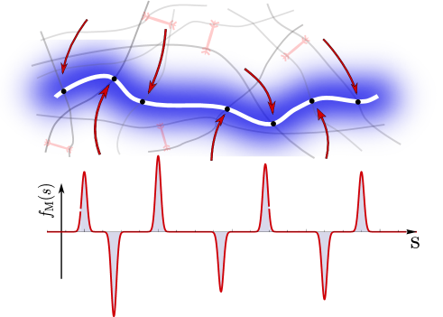
In the following, we lay out a framework to describe fluctuations of a semiflexible probe filament Kratky and Porod (1949); Aragon and Pecora (1985); Goldstein and Langer (1995); Hallatschek et al. (2007), which is embedded in a motor-activated network MacKintosh and Levine (2008); Levine and MacKintosh (2009); Osmanović and Rabin (2017). We assume the probe filament to be weakly-bending, such that we can focus on the transverse coordinate $r_{\perp}(s,t)$, where the arclength $0<s<L$ parametrizes the backbone, as shown in Fig. 13. The overdamped dynamics of such a probe filament is governed by a balance of (i) viscous and elastic forces of the surrounding viscoelastic medium, (ii) bending forces, (iii) thermal agitation, and (iv) motor-induced fluctuations, which read in this order as

$$\int\limits_{-\infty}^{t}\,\mathrm{d}t^{\prime}\,\alpha(t-t^{\prime})r_{\perp}(s,t^{\prime})+\kappa\frac{\partial^{4}r_{\perp}}{\partial t^{4}}(s,t) =\xi(s,t)+f_{\text{M}}(s,t).$$ (45)

Terms on the left describe relaxation, while terms on the right contain stochastic contributions. For a predominantly elastic network, we can use the generalized Stokes equation, $\hat{\alpha}(\omega)=k_{0}\hat{G}(\omega)$ to approximate the viscoelastic kernel on the left hand side as $\hat{G}=G_{0}+i\eta\omega$, i.e. as a Kelvin-Voigt-type viscoelastic solid. The factor $k_{0}$ has a geometrical origin, and is given by $k_{0}\approx 4\pi/\ln(L/d)$ for an infinitesimal rod segment of diameter $d$ Howard (2002). In a crosslinked actin network this approximation is reasonable for low frequencies typically below roughly $100\,\text{Hz}$, beyond which the network modulus exhibits a characteristic stiffening with frequency Koenderink et al. (2006); Mizuno et al. (2009); Guo et al. (2014). When the network is described as such a simple viscoelastic solid, the thermal noise is given by a Gaussian white-noise process $\xi(s,t)$, to which we add independent actively induced forces $f_{\text{M}}(s,t)$, specified in detail further below.

Bending forces can be conveniently studied from the perspective of bending modes of the probe filament. Following the approach in Gladrow et al. (2016, 2017), a description in terms of bending modes can be obtained from a decomposition of the backbone coordinates into orthogonal dynamic modes $r_{\perp}(s,t)=L\sum_{q}a_{q}(t)y_{q}(s)$ Aragon and Pecora (1985); Gittes et al. (1993); Brangwynne et al. (2007a). In this coordinate system, the multiscale character of probe filaments becomes apparent: each bending mode amplitude $a_{q}(t)$ is sensitive to a lengthscale corresponding to its wavelength. The precise form of bending modes, however, depends on the boundary conditions of the filament. The simplest case is a filament with zero transverse deflections at its end, where classical sine-modes $y_{q_{m}}(s)=\sqrt{2/L}\sin(q_{m}s)$ form an orthonormal set. Importantly, these modes are independent in equilibrium, due to their orthogonality. For fixed-end modes, mode number $m\in\{1,2,3,...\}$ and wave-vector $q$ are related via $q(m)=m\pi/L$. The relaxational timescale of each mode is set by a balance between both elastic and viscous forces of the network and the bending rigidity of the filament. For inextensible filaments in purely viscous environments, this results in a strongly length-dependent decay

$$\tau_{q} =\frac{\eta}{\kappa q^{4}/k_{0}+G_{0}},$$ (46)

In the linear-response regime, we obtain the mode-response function to transverse deflections, $\chi_{q}(t)$, in fourier space $\hat{\chi}_{q}(\omega)=(\hat{\alpha}(\omega)+\kappa q^{4})^{-1}$. This response function is related to mode variances in equilibrium via the mode fluctuation-dissipation theorem

$$\langle\left|\hat{a}_{q}(\omega)\right|^{2}\rangle =\frac{2k_{B}T}{L^{2}\omega}\hat{\chi}^{\prime\prime}_{q}(\omega).$$ (47)

Bending modes are thus ideally suited to not only detect motor activity, but also to measure their spatial and temporal characteristics. Perhaps for these reasons, bending mode fluctuations have been the subject of a number of studies in biological non-equilibrium systems.

In a study by Brangwynne et al. Brangwynne et al. (2008b), fluorescently labelled microtubuli were used to probe the active fluctuations in actin-myosin gels. The persistence lengths of microtubuli is on the order of millimeters Gittes et al. (1993), such that these filaments can be treated effectively as rigid on microscopic lengthscales under thermal conditions. By contrast, in actin-myosin gels, microtubuli exhibit significant fluctuations, caused by contractions of myosin, which deform the network in which the microtubules are embedded. A quantitative analysis of thermal bending mode fluctuations reveals a $q^{-4}$-decay in actin networks (without myosin). By contrast, adding myosin not only increases the amplitudes of fluctuations, but also results in a breakdown of the standard mode decay (see Eq. (46). The spatial extent of individual indentations in motor-agitated microtubuli can be used to extract forces induced by myosing. These force range between $0-30$ pN, in accord with more recent studies in live cells Guo et al. (2014); Fakhri et al. (2014). Importantly, the results also suggest a very narrow profile of the force exerted on the microtubules. Furthermore, in the cell cortex, microtubules often appear considerably more curved, despite their rigidity. Indeed, this curved microtubule structure is not due to temporal bending fluctuations of the microtubule, but rather results from geometrical constraints that randomly deflect the microtubule tip during polymerization Brangwynne et al. (2007b).

Motivated by these experimental observations, we can model the motor-induced force, exerted on the probe at the points where it is coupled elastically to the network, as a superposition of all active forces in the environment:

$$f_{\text{M}}(s,t)=\sum\limits_{n}\,f_{n}(s,t),$$ (48)

where each $f_{n}(s,t)$ denotes the force contribution from active motors, which affect the filament at the $n_{\rm th}$ entanglement point. Active forces have a characteristic spatial decay, since myosin motors exert forces in dipoles rather than in single directions Yuval and Safran (2013). The model in Eq. (48) does not account for such details; its main purpose is to provide a non-uniform force background $f(s)$ along the backbone $s$.

Measurements of myosin dynamics have revealed a Lorentzian power spectrum MacKintosh and Levine (2008); Mizuno et al. (2009). A simple on-off telegraph process $\mathcal{T}(t)$ is in accord with these observations and appears to be adequate to model the stochastic force dynamics of individual motors. Taking furthermore into account the narrow profile of motor forces inferred from experiments Brangwynne et al. (2008b), we arrive at a model for motor-induced forces, which reads $f_{n}(s,t)=f_{n}\delta(s-s_{n})\mathcal{T}_{n}(t)$. Here $\mathcal{T}_{n}(t)$ is a telegraph process with exponential decorrelation $\langle\mathcal{T}(t)\mathcal{T}(t^{\prime})\rangle=C_{2}\rm{exp}(-|t-t^{\prime}|/\tau_{M})$.

Figure 14: Mode amplitude variations in fluctuating microtubules embedded in actin-myosin gels over mode number $q$. A) In ATP-depleted gels (purely thermal noise), mode variances follow a power law decay. B) Active fluctuations result in enhanced mode variances in accord with the theory In Fig. 15. At high $q$-values measurement noise leads to an increase in mode variances. Adapted from Brangwynne et al. (2008b).

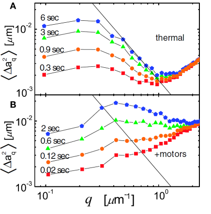
Using this simple description for the stochastic behavior of motor-generated forces together with Eq. (47), we compute the mode correlator, which decomposes into active and thermal contributions: $\langle a_{q}(t)a_{w}(t^{\prime})\rangle=\langle a_{q}(t)a_{w}(t^{\prime})\rangle^{\text{Th}}+\langle a_{q}(t)a_{w}(t^{\prime})\rangle^{\text{M}}$, given by

$$\langle a_{q}(t)a_{w}(t^{\prime})\rangle^{\text{Th}} =\frac{k_{B}T\tau_{q}}{L^{2}\gamma}\delta_{q,w}e^{-\frac{\left|t-t^{\prime}\right|}{\tau_{q}}}$$ (49)

$$\langle a_{q}(t)a_{w}(t^{\prime})\rangle^{\text{M}} =\frac{1}{L^{2}\gamma^{2}}\mathbf{F}_{q,w}C_{2}\mathcal{C}_{q,w}\left(t-t^{\prime}\right).$$ (50)

$\mathbf{F}_{q,w}$ specifies the geometry of motor-induced forces in mode space and is defined by $\mathbf{F}_{q,w}=\sum_{n}f_{n}^{2}y_{q}\left(s_{n}\right)y_{w}\left(s_{n}\right)$, where the sum runs over the filament-network contacts. The function $\mathcal{C}_{q,w}(\Delta t)$ denotes the temporal decorrelation of active mode fluctuations. In contrast to thermal equilibrium, active fluctuations decay as a double exponential

$$\mathcal{C}_{q,w}(t-t^{\prime}) =\tau_{q}\tau_{w}\left(\frac{e^{-\frac{\lvert t-t^{\prime}\rvert}{\tau_{\text{M}}}}}{\left(1-\frac{\tau_{q}}{\tau_{\text{M}}}\right)\left(1+\frac{\tau_{w}}{\tau_{\text{M}}}\right)}\right.$$

$$\left.-2\frac{\tau_{q}}{\tau_{\text{M}}}\frac{e^{-\frac{\lvert t^{\prime}-t\rvert}{\tau_{q}}}}{\left(1-\left(\frac{\tau_{q}}{\tau_{\rm M}}\right)^{2}\right)\left(1+\frac{\tau_{w}}{\tau_{q}}\right)}\right),$$ (51)

which indicates a competition between two decorrelating processes: mode relaxation and the internal decorrelation of the motor state. The correlator is not symmetric in the indices $q$ and $w$ as can be seen from Eq. (51), which results in a breaking of Onsager’s time-reversal symmetry Gladrow et al. (2017).

This double exponential in Eq. (51) is the footprint of colour of the noise process, which we use to describe motor-induced forces. The $q^{-4}$-decay of mode amplitudes relaxation times, $\tau_{q}$, levels off around $\tau_{\text{M}}$ as shown in Fig. 15C. This saturation occurs because modes cannot decorrelate faster than the force that is driving them. Under coloured noise, the relaxation times cannot be directly inferred from decorrelation. This is indeed confirmed in Brownian dynamics simulations of filaments subject to active fluctuations Gladrow et al. (2016). To further illustrate these results, simulations of mode variances over mode vector in passive (Fig.15A) and active (Fig.15B) networks are shown together with theoretical predictions from Eqs. (49,50). For comparison, experimentally obtained mode variances Brangwynne et al. (2008b) are plotted over $q$ in Fig. 14. As one would expect, in both cases mode variances are elevated in active environments.

Figure 15: Mode fluctuations under (A) purely thermal agitated and (B) under additional influence of motor-induced forces. C) Convergence of mode decorrelation times onto the motor timescale. Different colors correspond to the different times $\Delta t$ shown in the legend in panel (A). Adapted from Gladrow et al. (2016).

Figure 16: Steady-state probability currents in mode space. A) Projection of the multidimensional current on the mode amplitude pair $a_{1}$ and $a_{3}$. B) The same current in three dimensions $a_{1}$, $a_{3}$, and $a_{5}$. Due to the geometry of probe-network interactions in this example, only modes of similar number parity (e.g. odd-odd) couple. Adapted from Gladrow et al. (2016).

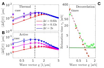
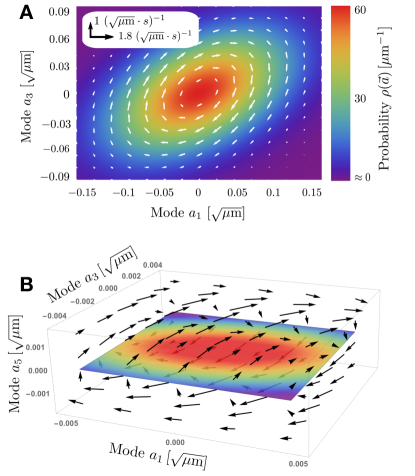
In the long time regime $t\gg\tau_{\text{M}}$, motor forces effectively appear as sources of white-noise. In this ‘white-noise limit’, the motor correlator converges to a $\delta$-function, $\langle\Delta\mathcal{T}(t)\Delta\mathcal{T}(t^{\prime})\rangle\to C_{2}/2\tau_{\text{M}}\delta(t-t^{\prime})$ with a factor $\tau_{\text{M}}$, which remains only as a scale of the variance of the motor process. The mode correlation function in the white-noise limit can be derived by a series expansion of $\mathcal{C}_{q,w}(t)$, which yields

$$\langle a_{q}(t)a_{w}(t^{\prime})\rangle^{\text{M}} =\frac{C_{2}\tau_{M}}{L^{2}\gamma^{2}}\mathbf{F}_{q,w}\frac{\tau_{q}\tau_{w}}{\tau_{q}+\tau_{W}}\delta(t-t^{\prime}).$$ (52)

We can now contract the thermal and motor-white noise processes into a single process $\psi(t)$, with a correlator $\langle\psi_{q}(t)\psi_{w}(t^{\prime})\rangle=\left(4k_{B}T\gamma\delta_{q,w}+C_{2}\tau_{\text{M}}\mathbf{F}_{q,w}\right)\frac{\delta\left(t-t^{\prime}\right)}{2L^{2}}$.

It is useful at this stage to compare this scenario with that described in Sec. III.1: Here, mode variables are independent, but are subject to noise with a cross-mode correlations, such that different modes are simultanously excited by a motor event. By constrast, thermal noise is uniform in amplitude and uncorrelated throughout the system, giving rise to independent stochastic forces in mode-space. As we discussed in Sec. III.1, a correlation in the external noise in one coordinate system, may appear as a “temperature” gradient in different coordinates. It is this mechanism, which gives rise to a probability flux in mode space, which breaks detailed balance in the fluctuations of the probe filament. In other words, a motor-induced force background $\langle f_{\text{M}}(s,t)\rangle_{\text{temporal}}=\lim_{t_{1}\to\infty}\int_{t_{0}}^{t_{1}}\mathrm{d}tf_{\text{M}}(s,t)$ (see lower panel in Fig. 13), which varies along the filament, will lead to a breaking of detailed balance in a hyperplane spanned by the affected modes.

The magnitude and structure of this probability current, is given as a solution of the multivariate Fokker-Planck equation $\partial_{t}\rho(\vec{a},t)=-\vec{\nabla}\cdot\vec{j}(\vec{a},t)$ in mode space. The probability current, $\vec{j}(\vec{a})$, can be written in steady-state as

$$\vec{j}(\vec{a})=(\mathbf{K}+\mathbf{D}\mathbf{C}^{-1})\vec{a}\rho(\vec{a})\equiv\mathbf{\Omega}\vec{a}\rho(\vec{a}),$$ (53)

where $\mathbf{K}_{q,w}=-1/\tau_{q}\delta_{q,w}$ is the deterministic matrix which defines the linear force field, and $\mathbf{D}$ and $\mathbf{C}$ represent respectively the diffusion and covariance matrices. Within this linear description, $\mathbf{\Omega}$ is the matrix that captures the structure of the current Weiss (2003, 2007). A rotational probability current in the Fokker-Planck picture is associated with a net rotation of variables in the Langevin description: On average, mode amplitudes cycle around the origin, when detailed balance is broken in steady-state, as illustrated in Fig. 16.

The circular character of the current is reflected mathematically by the skew-symmetry of $\mathbf{\Omega}^{T}=-\mathbf{\Omega}$ in the coordinate system where $\tilde{\mathbf{C}}=\mathbf{1}$ (“correlation-identity coordinates”). This can be seen from Eq. (40), which dictates that $\tilde{\mathbf{K}}+\tilde{\mathbf{K}}^{T}=-2\tilde{\mathbf{D}}$ in this system, such that $\tilde{\mathbf{\Omega}}=\frac{1}{2}\left(\tilde{\mathbf{K}}-\tilde{\mathbf{K}}^{T}\right)$. The eigenvalues of any skew-symmetric matrix $\mathbf{M}$ are either zero or purely imaginary, with the latter leading to rotational currents in a hypothetical dynamical system described by $\dot{\vec{x}}=\mathbf{M}\vec{x}$. Moreover, since $\text{tr}\left(\mathbf{\Omega}\right)=0$, in two dimensions, this implies that the eigenvalues can be rewritten as $\lambda_{1,2}=\pm i\omega$. In a steady-state, the probability current $\vec{j}$ (in any dimension) has to be orthogonal to the gradient of the density $\rho(\vec{a},t)$, since $\vec{\nabla}\cdot\vec{j}(\vec{a})=\rho(\vec{a})\vec{\nabla}\cdot(\mathbf{\Omega}\vec{a})+\left(\mathbf{\Omega}\vec{a}\right)\cdot\vec{\nabla}\vec{\rho}(\vec{a})=\partial_{t}\rho=0$. The first term must be zero, since it is proportional to $\text{tr}\left(\mathbf{\Omega}\right)\vec{a}$, so that the second term has to vanish as well. This, however, implies that $\vec{\nabla}\rho\perp\mathbf{\Omega}\vec{a}$: the gradient of the density must be perpendicular to the flow field. In a linear system, the probability density is always Gaussian $\rho\propto e^{-\frac{1}{2}\vec{a}^{T}\mathbf{C}^{-1}\vec{a}}$, such that the flow field must have an ellipsoidal structure Weiss (2003). In correlation-identity coordinates, where the density has a radial symmetry, the profile of $\tilde{\vec{j}}$ would thus be purely azimuthal, and its magnitude would represent an angular velocity. An average over the angular movements $\langle\dot{\varphi}\rangle$ of the mode vector $\vec{a}(t)$ in the plane will yield the cycling frequency. The imaginary part of the positive eigenvalue of $\mathbf{\Omega}$ must therefore represent the average cycling frequency of the mode vector in the plane.

In a reduced two-dimensional system consisting only of $a_{q}(t)$ and $a_{w}(t)$, the cycling frequency can be calculated analytically and reads

$$\omega_{q,w}^{\text{2D}}=\frac{\left(\tau_{q}-\tau_{w}\right)\mathbf{F}_{q,w}}{\sqrt{\tau_{q}\tau_{w}\left(\left(\tau_{q}+\tau_{w}\right)^{2}\beta-4\tau_{q}\tau_{w}\mathbf{F}_{q,w}^{2}\right)}}.$$ (54)

where $\beta=((\frac{2k_{B}T\gamma}{C_{2}\tau_{M}})^{2}+\frac{2k_{B}T\gamma}{C_{2}\tau_{\text{M}}}\mathbf{F}_{q,q}+\mathbf{F}_{w,w})+\mathbf{F}_{w,w}\mathbf{F}_{q,q})$.

Interestingly, Eq. (54) shows that in the case of equal relaxation times $\tau_{q}=\tau_{w}$, the cycling frequency would be zero and thus, detailed balance would be restored, regardless of differences between the modes in motor-induced fluctuations. This hints at an important role of relaxation times in determining the shape of the current in multidimensional systems. Furthermore, the denominator of Eq. (54) shows how an increase in overall temperature $T$ could mask broken detailed balance by reducing the cycling frequency.

In summary, filaments as multi-scale and multi-variable probes offer a novel perspective on non-equilibrium phenomena in active matter and could be used in the future as “non-equilibrium antennae”. As we illustrated in this section, a heterogeneous force background $f_{\text{M}}(s,t)$ created by motor-induced fluctuations leads to a breaking of detailed balance in mode space of embedded filaments. The intricate structure of the probability current in steady-state may contain a wealth of information about the geometric and, perhaps, temporal structure of impinging active forces.

The theory laid out in this section can be generalized to other objects, such as membranes Strey et al. (1995); Granek (1997); Betz et al. (2009); Turlier et al. (2016). In principle, the membrane mode decomposition described in Sec. II could be used to detect a breaking of detailed balance, since active processes in the cortex of red blood cells might result in noise input that correlates over different membrane modes.

V Outlook

The examples discussed in this review illustrate how experimental measurements of nonequilibrium activity and irreversibility can provide a deeper conceptual understanding of active biological assemblies and non-equilibrium processes in cells. In many cases, non-equilibrium fluctuations have successfully been identified and quantified using the combination of active and passive microrheology techniques to study the violation of the fluctuation-dissipation theorem, Mizuno et al. (2007); Turlier et al. (2016). Such studies can for instance reveal the force spectrum inside cells, Guo et al. (2014). However, these approaches require invasive micromechanical manipulation. Furthermore, a complete generalization of the fluctuation-dissipation theorem for non-equilibrium system is still lacking, such that the response of a non-equilibrium system can not be inferred from it’s spontaneous fluctuations. However, this does not mean that the fluctuations of a non-equilibrium steady state do not contain valuable information about the nature of the system. Indeed, non-invasive approaches to measure broken detailed balance from stochastic dynamics have now been establishes to reveal phase space currents in mesoscopic degrees of freedom of biological systems, Battle et al. (2016). It remains an open question what information can be inferred about the underlying system from such phase space currents, Gladrow et al. (2016, 2017). However, recently derived theoretical relations for energy dissipation and entropy production to characterize non-equilibrium activity are finding traction in various biological systems such as molecular motors and chemical control systems Hartich et al. (2015); Lan et al. (2012); Mehta and Schwab (2012); Barato and Seifert (2015).

Taken together, the research discussed in this review illustrate that the gap between fundamental approaches in stochastic thermodynamics and its application to real biological system is slowly closing. Indeed, studies of biological active matter are not only yielding insights in non-equilibrium physics, they have also suggested conceptually novel mechanisms in cell biology. For instance, the collective effect of forces exerted by molecular motors has been implicated in intracellular transport and positioning of the nucleus Caspi et al. (2000); Brangwynne et al. (2009); Fakhri et al. (2014); Guo et al. (2014); Almonacid et al. (2015). This novel mode of transport, known as active diffusion, is thought to complement thermal diffusion and directed, motor-driven modes of transport in cells. Another intriguing example is the role of DNA-binding ATPases, which have been suggested to be capable of generating forces on the chromosomes through a DNA-relay mechanism Lim et al. (2014) or loop extrusion Wang et al. (2013); Wilhelm et al. (2015). ATP- or GTPases can also interact with membranes or DNA to play a role in pattern forming systems Huang et al. (2003); Frey et al. (2017); Halatek and Frey (2012), for instance in the Min system in E. coli and CDC42 in yeast. In these systems, certain proteins can switch irreversibly between different conformational states, affecting their affinity to be in the cytosol or the membrane. This, together with nonlinear interactions between these different proteins, can result in non-equilibrium dynamic pattern formation.

Another important example in this respect is how cells break symmetry to form a polarity axes. Intracellular myosin activity has been implicated in establishing a sense of direction (’polarity’) in cells. In order to divide, cells must ’decide’ on the axis of the mytotic spindle, which is a crucial part of the cell division apparatus Grill et al. (2001); Grill (2003); Pecreaux et al. (2006); Ou et al. (2010). Cortical flows resulting from asymmetries in myosin activity have been shown to effectively polarize C.elegans cells and break the initial cellular symmetry Mayer et al. (2010).

Non-equilibrium phenomena also emerge at the multicellular scale: Groups of motile cells exhibit collective active dynamics, such as flocking, swarming, non-equilibrium phase transitions or the coordinated movements of cells during embryonic developments  Thutupalli et al. (2015); Peruani et al. (2012). More broadly, non-equilibrium physics is emerging as a guiding framework to understand phenomena related to self-replication and adaptation England (2013, 2015); Perunov et al. (2016), the origin of life (see for example Frauenfelder et al. (1999); Agerschou et al. (2017)), as well as synthetic life-like systems (See Schwille and Diez (2009) and references therein).