Weak localization of magnons in a disordered two-dimensional antiferromagnet

Abstract

We propose the weak localization of magnons in a disordered two-dimensional antiferromagnet. We derive the longitudinal thermal conductivity $\kappa_{xx}$ for magnons of a disordered Heisenberg antiferromagnet in the linear-response theory with the linear-spin-wave approximation. We show that the back scattering of magnons is enhanced critically by the particle-particle-type multiple impurity scattering. This back scattering causes a logarithmic suppression of $\kappa_{xx}$ with the length scale in two dimensions. We also argue a possible effect of inelastic scattering on the temperature dependence of $\kappa_{xx}$. This weak localization is useful to control turning the magnon thermal current on and off.

Introduction. The Anderson localization is an impurity-induced localization of electrons Anderson . Its effects depend on the dimension of the system and the symmetry of the Hamiltonians RG-4persons ; Gorkov ; Lee ; Hikami . The understanding has been advanced substantially by the theory in the weak-localization regime, where the effects of impurities can be treated as perturbation Gorkov ; Lee ; Hikami ; WeakLoc-review ; Nagaoka . For example, the weak-localization theory of a disordered two-dimensional electron system demonstrates the logarithmic temperature dependence of the resistivity, the negative magnetoresistance, and the antilocalization due to the spin-orbit coupling; those are experimentally confirmed exp-logT ; exp-NegativeMR ; exp-SOC . That theory also reveals the Anderson localization originates from the critical back scattering due to the multiple electron-electron scattering under time-reversal symmetry WeakLoc-review .

Since the similar argument may be applicable to magnons, quasiparticles in a magnet, the weak localization of magnons has the potential for a new avenue in spintronics. Among several possibilities, antiferromagnets are suitable because global time-reversal symmetry holds and because even nondisordered antiferromagnets have several applications Jungwirth . (In contrast to electron systems, local time-reversal symmetry is broken in any magnets due to the magnetic ordering.) Then the knowledge for disordered antiferromagnets will be useful for others, such as disordered ferromagnets, which break global time-reversal symmetry. As well as antiferromagnets, ferromagnets are useful for carrying information and energy Kajiwara ; Uchida ; Bauer .

Despite the above potential, it is unclear how impurities affect magnon transport even in the weak-localization regime. In particular, the weak-localization theory of magnons under global time-reversal symmetry will be highly desirable because the previous theories MagLoc1 ; MagLoc2 ; MagLoc3 ; MagLoc4 about the magnon localization analyze ferromagnetic cases, in which global time-reversal symmetry is broken. Although there is a previous theory MagLoc-exception about the magnon localization in an antiferromagnetic case, that does not study magnon transport. Since the existence of the back scattering is not sufficient to justify the localization, it is necessary to study magnon transport in disordered antiferromagnets. In particular, it is essential to clarify whether the weak localization occurs or not in the presence of global time-reversal symmetry without local time-reversal symmetry and how the weak localization of magnons is characterized by an observable quantity.

In this Rapid Communication we formulate the longitudinal thermal conductivity $\kappa_{xx}$ of magnons in a disordered Heisenberg antiferromagnet, and show disorder effects in the weak-localization regime. Our formulation is based on the linear-response theory Luttinger ; Oji-Streda ; Tatara with the linear-spin-wave approximation Anderson-SW . In our model, disorder is induced by partial substitution for magnetic ions [Fig. 1(b)], and its main effect is considered as changing the value of the Heisenberg interaction. We show that the particle-particle-type multiple impurity scattering of magnons causes the critical back scattering for any dimension and any spin quantum number $S$. Most importantly, this critical back scattering drastically suppresses the magnon thermal flow in two dimensions. We also argue a possible temperature dependence of $\kappa_{xx}$ in the presence of inelastic scattering. We finally discuss the validity of our theory and implications of experiments and theories. Throughout this paper we set $k_{\textrm{B}}=1$ and $\hbar=1$.

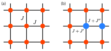
Figure 1: Schematic pictures of a lattice (a) without and (b) with disorder. An orange circle represents a magnetic ion, and a blue circle represents a different one. $J$, $J+J^{\prime}$, and $J+J^{\prime\prime}$ are the Heisenberg interactions between orange circles, between orange and blue circles, and between blue circles.

Model. We begin to construct a model for a disordered antiferromagnet. Our model Hamiltonian is $\hat{H}=\hat{H}_{0}+\hat{H}_{\textrm{imp}}$, where $\hat{H}_{0}$ is the Hamiltonian without impurities and $\hat{H}_{\textrm{imp}}$ is the impurity Hamiltonian. $\hat{H}_{0}$ consists of the antiferromagnetic Heisenberg interaction between nearest-neighbor sites and the magnetic anisotropy,

$$\hat{H}_{0}=2J\sum\limits_{\langle\bm{i},\bm{j}\rangle}\hat{\bm{S}}_{\bm{i}}\cdot\hat{\bm{S}}_{\bm{j}}-D\Bigl{[}\sum\limits_{\bm{i}\in A}(\hat{S}^{z}_{\bm{i}})^{2}+\sum\limits_{\bm{j}\in B}(\hat{S}^{z}_{\bm{j}})^{2}\Bigr{]},$$ (1)

where $\bm{i}\in A$ and $\bm{j}\in B$ for the $A$ or $B$ sublattice, and $\textstyle\sum_{\langle\bm{i},\bm{j}\rangle}=Nz/2$ with $N$, as the number of sites, and $z$, as the coordination number; the numbers of $A$ and $B$ are equal. We assume that $J(>0)$ is much larger than $D(>0)$. Then we construct $\hat{H}_{\textrm{imp}}$ as follows. We first assume that one kind of disorder is partial substitution for magnetic ions (see Fig. 1), and its main effect is to modify the value of the exchange interaction; for simplicity, we neglect the disorder effect from the magnetic anisotropy because its magnitude will be much smaller. Thus $\hat{H}_{\textrm{imp}}$ becomes

$$\hat{H}_{\textrm{imp}}=2\sum\limits_{\langle\bm{i},\bm{j}\rangle}\Delta J_{\bm{i}\bm{j}}^{(\textrm{imp})}\hat{\bm{S}}_{\bm{i}}\cdot\hat{\bm{S}}_{\bm{j}},$$ (2)

with $\Delta J_{\bm{i}\bm{j}}^{(\textrm{imp})}=J^{\prime}$ for $\bm{i}\in A_{\textrm{imp}}$, $\bm{j}\in B_{0}$ or for $\bm{i}\in A_{0}$, $\bm{j}\in B_{\textrm{imp}}$, and $\Delta J_{\bm{i}\bm{j}}^{(\textrm{imp})}=J^{\prime\prime}$ for $\bm{i}\in A_{\textrm{imp}}$, $\bm{j}\in B_{\textrm{imp}}$; $A_{0}$ and $B_{0}$ represent $A$ and $B$ sublattice for orange circles in Fig. 1(b), while $A_{\textrm{imp}}$ and $B_{\textrm{imp}}$ represent those for blue ones; the numbers of $A_{\textrm{imp}}$ and $B_{\textrm{imp}}$ are equal. In a similar way to electron systems AGD we suppose that impurities are randomly distributed. Also, we assume that $J^{\prime}$ and $J^{\prime\prime}$ are much smaller than $J$. Thus the main terms of Eq. (2) come from the mean-field-type terms,

$$\hat{H}_{\textrm{imp}}=-\sum\limits_{\bm{i}\in A_{\textrm{imp}}}V_{\textrm{imp}}\hat{S}_{\bm{i}}^{z}+\sum\limits_{\bm{j}\in B_{\textrm{imp}}}V_{\textrm{imp}}\hat{S}_{\bm{j}}^{z},$$ (3)

where $V_{\textrm{imp}}=2Sz^{\prime\prime}J^{\prime\prime}$ with $z^{\prime\prime}$, the coordination number for $J+J^{\prime\prime}$. Here we have neglected the other mean-field-type terms, $-\sum{}_{\bm{i}\in A}V\hat{S}_{\bm{i}}^{z}+\sum{}_{\bm{j}\in B}V\hat{S}_{\bm{j}}^{z}$ ($V=2Sz^{\prime}J^{\prime}$ with $z^{\prime}$, the coordination number for $J+J^{\prime}$), because those lead to the same effect as the magnetic anisotropy in the linear-spin-wave Hamiltonian; the effect of the terms in Eq. (3) is different due to the limit of the sum of sites.

We next express our Hamiltonian in terms of magnon operators. For that purpose, we use the linear-spin-wave approximation Anderson-SW for a collinear antiferromagnet. As a result, Eq. (1) becomes

$$\hat{H}_{0}= \sum\limits_{\bm{q}}\sum\limits_{l,l^{\prime}=A,B}\epsilon_{ll^{\prime}}(\bm{q})\hat{x}^{\dagger}_{\bm{q}l}\hat{x}_{\bm{q}l^{\prime}},$$ (4)

where $\epsilon_{AA}(\bm{q})=\epsilon_{BB}(\bm{q})=2S(Jz+D)$ and $\epsilon_{AB}(\bm{q})=\epsilon_{BA}(\bm{q})=2SJ\sum_{j=1}^{z}e^{i\bm{q}\cdot\bm{r}_{j}}$, and Eq. (3) becomes

$$\hat{H}_{\textrm{imp}}= \sum\limits_{\bm{q},\bm{q}^{\prime}}\sum\limits_{l=A,B}V^{\textrm{imp}}_{l}(\bm{q}-\bm{q}^{\prime})\hat{x}_{\bm{q}l}^{\dagger}\hat{x}_{\bm{q}^{\prime}l},$$ (5)

where $V^{\textrm{imp}}_{l}(\bm{Q})=V_{\textrm{imp}}\frac{2}{N}\sum_{\bm{i}\in l_{\textrm{imp}}}e^{i\bm{Q}\cdot\bm{i}}$. Here $\sum_{\bm{q}}$ is the sum of momentum in the first Brillouin zone; the magnon operators fulfill $\hat{x}_{\bm{q}A}=\hat{a}_{\bm{q}}$ and $\hat{x}_{\bm{q}B}=\hat{b}^{\dagger}_{\bm{q}}$ with $\hat{a}_{\bm{q}}$, the annihilation operator for the $A$ sublattice, and $\hat{b}^{\dagger}_{\bm{q}}$, the creation operator for the $B$ sublattice. Then we obtain the eigenvalues of Eq. (4) using the Bogoliubov transformation Anderson-SW : $\hat{H}_{0}=\sum_{\bm{q}}\sum_{\nu=\alpha,\beta}\epsilon_{\bm{q}}\hat{x}_{\bm{q}\nu}^{\dagger}\hat{x}_{\bm{q}\nu}$, where $\nu$ is the band index for the $\alpha$ and $\beta$ bands, $\epsilon_{\bm{q}}=\sqrt{\epsilon_{AA}(\bm{q})^{2}-\epsilon_{AB}(\bm{q})^{2}}$ and $\hat{x}_{\bm{q}l}=\sum_{\nu=\alpha,\beta}U_{l\nu}(\bm{q})\hat{x}_{\bm{q}\nu}$ with $U_{A\alpha}(\bm{q})=U_{B\beta}(\bm{q})=\cosh\theta_{\bm{q}}$, $U_{A\beta}(\bm{q})=U_{B\alpha}(\bm{q})=-\sinh\theta_{\bm{q}}$, and $\tanh 2\theta_{\bm{q}}=\frac{\epsilon_{AB}(\bm{q})}{\epsilon_{AA}(\bm{q})}$.

Situation. As magnon transport in our disordered antiferromagnet, we consider $\kappa_{xx}$, given by $j_{\textrm{Q}}^{x}=\kappa_{xx}(-\partial_{x}T)$. Here $j_{\textrm{Q}}^{x}$ is the thermal current density, and $(-\partial_{x}T)$ is the temperature gradient; for magnons the thermal current is equal to the energy current. We focus on the thermal transport rather than the charge transport, considered for the localization of electrons WeakLoc-review ; Nagaoka , because the charge transport is absent in magnets, magnetically ordered insulators. Furthermore, we consider $\kappa_{xx}$ because $\kappa_{xx}$ is finite even without external magnetic fields. To analyze $\kappa_{xx}$, we assume that the temperature gradient is so smooth that the local equilibrium is reached, that is, the local temperature is definable. We also assume that the local energy conservation holds. Those assumptions are standard ones Mahan-text ; Luttinger ; Oji-Streda ; Tatara .

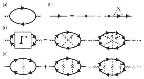
Figure 2: Feynman diagrams of (a) $\kappa_{xx}^{(\textrm{Born})}$, (b) the Dyson equation, (c) $\Delta\kappa_{xx}$ and (d) the contribution from the particle-hole-type vertex corrections. Bold arrows and thin arrows denote the magnon Green’s functions after taking the impurity averaging and the magnon Green’s functions without impurities; a dotted line denotes the impurity scattering.

Linear-response theory. Using the linear-response theory Luttinger ; Oji-Streda ; Tatara ; Eliashberg ; NA-Ch ; NA-AHESHE , we can express $\kappa_{xx}$ as

$$\kappa_{xx}=\frac{1}{T}\lim\limits_{\omega\rightarrow 0}\dfrac{K_{xx}^{(\textrm{R})}(\omega)-K_{xx}^{(\textrm{R})}(0)}{i\omega},$$ (6)

where $K_{xx}^{(\textrm{R})}(\omega)=K_{xx}(i\Omega_{n}\rightarrow\omega+i0+)$ with $\Omega_{n}=2\pi Tn$ $(n=0,\pm 1,\pm 2,\cdots)$, bosonic Matsubara frequency, and $K_{xx}(i\Omega_{n})=\frac{1}{N}\int^{T^{-1}}_{0}d\tau e^{i\Omega_{n}\tau}\langle\textrm{T}_{\tau}\hat{J}_{\textrm{E}}^{x}(\tau)\hat{J}_{\textrm{E}}^{x}\rangle$ with $T_{\tau}$, a $\tau$-ordering operator Mahan-text . Since the energy current operator can be derived by using the local energy conservation Mahan-text , we can derive $\hat{J}_{\textrm{E}}^{x}$ of our model Supp ,

$$\hat{J}_{\textrm{E}}^{x}=\sum\limits_{\bm{q}}\sum\limits_{l,l^{\prime}=A,B}e_{ll^{\prime}}^{x}(\bm{q})\hat{x}_{\bm{q}l}^{\dagger}\hat{x}_{\bm{q}l^{\prime}},$$ (7)

with $e_{AA}^{x}(\bm{q})=-e_{BB}^{x}(\bm{q})=\frac{\partial\epsilon_{AB}(\bm{q})}{\partial q_{x}}\epsilon_{AB}(\bm{q})$ and $e_{AB}^{x}(\bm{q})=e_{BA}^{x}(\bm{q})=\bm{0}$. Then, by using a field theoretical technique AGD ; Eliashberg ; NA-Ch ; NA-AHESHE , we obtain

$$\kappa_{xx}= \frac{1}{TN}\sum\limits_{\bm{q},\bm{q}^{\prime}}\sum\limits_{\{l_{1}\}}e_{l_{1}l_{2}}^{x}(\bm{q})e_{l_{3}l_{4}}^{x}(\bm{q}^{\prime})P\int^{\infty}_{-\infty}\frac{d\epsilon}{2\pi}\Bigl{[}-\frac{\partial n(\epsilon)}{\partial\epsilon}\Bigr{]}$$

$$\times\langle D_{l_{4}l_{1}}^{(\textrm{A})}(\bm{q}^{\prime},\bm{q},\epsilon)D_{l_{2}l_{3}}^{(\textrm{R})}(\bm{q},\bm{q}^{\prime},\epsilon)\rangle,$$ (8)

where $\sum{}_{\{l_{1}\}}\equiv\sum{}_{l_{1},l_{2},l_{3},l_{4}}$, $n(\epsilon)$ is the Bose distribution function, and $D_{l_{4}l_{1}}^{(\textrm{A})}(\bm{q}^{\prime},\bm{q},\epsilon)$ and $D_{l_{2}l_{3}}^{(\textrm{R})}(\bm{q},\bm{q}^{\prime},\epsilon)$, the advanced and retarded Green’s functions of magnons for $\hat{H}$ before taking the impurity averaging. (For the derivation, see the Supplemental Material Supp .) We have neglected the term including $\langle D_{l_{4}l_{1}}^{(\textrm{R})}(\bm{q}^{\prime},\bm{q},\epsilon)D_{l_{2}l_{3}}^{(\textrm{R})}(\bm{q},\bm{q}^{\prime},\epsilon)\rangle$ or $\langle D_{l_{4}l_{1}}^{(\textrm{A})}(\bm{q}^{\prime},\bm{q},\epsilon)D_{l_{2}l_{3}}^{(\textrm{A})}(\bm{q},\bm{q}^{\prime},\epsilon)\rangle$ because the term in Eq. (8) is primary in the weak-localization regime WeakLoc-review ; Nagaoka .

Weak-localization theory. We formulate the weak-localization theory of our disordered antiferromagnet. That theory describes the disorder effects in the weak-localization regime, in which the magnitude of $V_{\textrm{imp}}$ is smaller than the magnon energy and the impurity concentration, $n_{\textrm{imp}}=\frac{N_{\textrm{imp}}}{N}$, is dilute. Since $V_{\textrm{imp}}$ comes from $J^{\prime\prime}$, we can apply the perturbation expansion of $\hat{H}_{\textrm{imp}}$ to Eq. (8). We can employ that expansion in a similar way to the longitudinal conductivity of electrons WeakLoc-review ; Nagaoka and reduce Eq. (8) to $\kappa_{xx}=\kappa_{xx}^{(\textrm{Born})}+\Delta\kappa_{xx}$. $\kappa_{xx}^{(\textrm{Born})}$ is $\kappa_{xx}$ without vertex corrections [Fig. 2(a)],

$$\kappa_{xx}^{(\textrm{Born})}= \frac{1}{TN}\sum\limits_{\bm{q}}\sum\limits_{\{l_{1}\}}e_{l_{1}l_{2}}^{x}(\bm{q})e_{l_{3}l_{4}}^{x}(\bm{q})P\int^{\infty}_{-\infty}\frac{d\epsilon}{2\pi}\Bigl{[}-\frac{\partial n(\epsilon)}{\partial\epsilon}\Bigr{]}$$

$$\times\bar{D}_{l_{4}l_{1}}^{(\textrm{A})}(\bm{q},\epsilon)\bar{D}_{l_{2}l_{3}}^{(\textrm{R})}(\bm{q},\epsilon),$$ (9)

and $\Delta\kappa_{xx}$ is the contribution from the particle-particle-type vertex corrections [Fig. 2(c)],

$$\Delta\kappa_{xx}= \frac{1}{TN}\sum\limits_{\bm{q},\bm{q}^{\prime}}\sum\limits_{\{l_{1}\}}\sum\limits_{l,l^{\prime}}e_{l_{1}l_{2}}^{x}(\bm{q})e_{l_{3}l_{4}}^{x}(\bm{q}^{\prime})P\int^{\infty}_{-\infty}\frac{d\epsilon}{2\pi}\Bigl{[}-\frac{\partial n(\epsilon)}{\partial\epsilon}\Bigr{]}\bar{D}_{l_{4}l^{\prime}}^{(\textrm{A})}(\bm{q}^{\prime},\epsilon)\bar{D}_{l_{2}l^{\prime}}^{(\textrm{R})}(\bm{q},\epsilon)\Gamma_{l^{\prime}l}(\bm{q}+\bm{q}^{\prime},\epsilon)\bar{D}_{ll_{1}}^{(\textrm{A})}(\bm{q},\epsilon)\bar{D}_{ll_{3}}^{(\textrm{R})}(\bm{q}^{\prime},\epsilon).$$ (10)

The contribution from the particle-hole type vertex corrections [Fig. 2(d)] will be negligible for our disordered antiferromagnet because of the similar argument to electron systems with inversion symmetry WeakLoc-review ; Nagaoka ; NA-AHESHE . Then the magnon Green’s functions in Eqs. (9) and (10) are determined from the Dyson equation [Fig. 2(b)]: $\bar{D}_{ll^{\prime}}^{(\textrm{R})}(\bm{q},\epsilon)=D_{ll^{\prime}}^{0(\textrm{R})}(\bm{q},\epsilon)+\sum_{l^{\prime\prime}}D_{ll^{\prime\prime}}^{0(\textrm{R})}(\bm{q},\epsilon)\Sigma_{l^{\prime\prime}}^{(\textrm{R})}(\epsilon)\bar{D}_{l^{\prime\prime}l^{\prime}}^{(\textrm{R})}(\bm{q},\epsilon)$, where $D_{ll^{\prime}}^{0(\textrm{R})}(\bm{q},\epsilon)$ is the retarded Green’s function without impurities and $\Sigma_{l}^{(\textrm{R})}(\epsilon)$ is the retarded self-energy, $\Sigma_{l}^{(\textrm{R})}(\epsilon)=\gamma_{\textrm{imp}}\sum{}_{\bm{q}}\bar{D}_{ll}^{(\textrm{R})}(\bm{q},\epsilon)$ with $\gamma_{\textrm{imp}}=\frac{2}{N}n_{\textrm{imp}}V_{\textrm{imp}}^{2}$; the advanced quantities are similarly determined. The vertex function in Eq. (10) is determined from the Bethe-Salpeter equation [Fig. 2(c)]: $\Gamma_{ll^{\prime}}(\bm{Q},\omega)=\gamma_{\textrm{imp}}^{2}\Pi_{ll^{\prime}}(\bm{Q},\omega)+\sum_{l^{\prime\prime}}\gamma_{\textrm{imp}}\Pi_{ll^{\prime\prime}}(\bm{Q},\omega)\Gamma_{l^{\prime\prime}l^{\prime}}(\bm{Q},\omega)$ with $\Pi_{ll^{\prime}}(\bm{Q},\omega)=\sum{}_{\bm{q}_{1}}\bar{D}_{ll^{\prime}}^{(\textrm{R})}(\bm{q}_{1},\omega)\bar{D}_{ll^{\prime}}^{(\textrm{A})}(\bm{Q}-\bm{q}_{1},\omega)$.

To proceed with the formulation as simple as possible, we introduce two simplifications. The first one is about the self-energy: we consider only the imaginary part. This is appropriate because its effect is essential for the localization WeakLoc-review ; Nagaoka . The other is about the Green’s functions: for positive frequencies we consider only the positive-pole contribution, whereas for negative frequencies we consider only the negative-pole contribution. For the more precise explanation, let us consider $D_{ll^{\prime}}^{0(\textrm{R})}(\bm{q},\epsilon)$. That for our model is given by

$$D_{ll^{\prime}}^{0(\textrm{R})}(\bm{q},\epsilon)=\frac{U_{l\alpha}(\bm{q})U_{l^{\prime}\alpha}(\bm{q})}{\epsilon-\epsilon_{\bm{q}}+i\delta}-\frac{U_{l\beta}(\bm{q})U_{l^{\prime}\beta}(\bm{q})}{\epsilon+\epsilon_{\bm{q}}+i\delta},$$ (11)

where $\delta\rightarrow 0+$. The above first and second terms provide the positive-pole and negative-pole contributions, respectively; the first and second terms are dominant for $\epsilon>0$ and $\epsilon<0$, respectively. We thus approximate $D_{ll^{\prime}}^{0(\textrm{R})}(\bm{q},\epsilon)$ for $\epsilon>0$ by the first term of Eq. (11), and $D_{ll^{\prime}}^{0(\textrm{R})}(\bm{q},\epsilon)$ for $\epsilon<0$ by the second term. Combining this and the first simplification with the Dyson equation, we obtain

$$\bar{D}_{ll^{\prime}}^{(\textrm{R})}(\bm{q},\epsilon)\sim\begin{cases}\dfrac{U_{l\alpha}(\bm{q})U_{l^{\prime}\alpha}(\bm{q})}{\epsilon-\epsilon_{\bm{q}}+i\tilde{\gamma}(\epsilon)}&(\epsilon>0),\\[10.0pt] -\dfrac{U_{l\beta}(\bm{q})U_{l^{\prime}\beta}(\bm{q})}{\epsilon+\epsilon_{\bm{q}}+i\tilde{\gamma}(-\epsilon)}&(\epsilon<0),\end{cases}$$ (12)

where $\tilde{\gamma}(\epsilon)=(\cosh^{4}\theta_{\bm{q}}+\sinh^{4}\theta_{\bm{q}})\gamma(\epsilon)$ with $\gamma(\epsilon)=n_{\textrm{imp}}V_{\textrm{imp}}^{2}\pi\rho(\epsilon)$; $\rho(\epsilon)$ is the density of states, and $\bm{q}$ of these hypobolic functions are determined by $\epsilon_{\bm{q}}=|\epsilon|$. The advanced quantities are simplified similarly.

The above simplifications enable us to proceed with the formulation in a similar way to the weak localization of electrons WeakLoc-review ; Nagaoka . First, we get a simple expression of $\kappa_{xx}^{(\textrm{Born})}$,

$$\kappa_{xx}^{(\textrm{Born})}\sim\frac{1}{TN}\sum\limits_{\bm{q}}\Bigl{(}\frac{\partial\epsilon_{\bm{q}}}{\partial q_{x}}\epsilon_{\bm{q}}\Bigr{)}^{2}\Bigl{[}-\frac{\partial n(\epsilon_{\bm{q}})}{\partial\epsilon_{\bm{q}}}\Bigr{]}\tilde{\tau}(\epsilon_{\bm{q}}),$$ (13)

where $\tilde{\tau}(\epsilon_{\bm{q}})=\tilde{\gamma}(\epsilon_{\bm{q}})^{-1}$. Due to the factor $[-\partial n(\epsilon_{\bm{q}})/\partial\epsilon_{\bm{q}}]$, the contributions for small $q=|\bm{q}|$ are dominant. Then, by estimating $\Pi_{ll^{\prime}}(\bm{Q},\omega)$ and $\Gamma_{ll^{\prime}}(\bm{Q},\omega)$ for small $Q=|\bm{Q}|$, we can demonstrate that $\Gamma_{ll^{\prime}}(\bm{Q},\omega)$ diverges in the limit $Q\rightarrow 0$. The brief outline of the estimates is as follows (for the details, see the Supplemental Material Supp ). First, by using Eq. (12) and performing the momentum sum in $\Pi_{ll^{\prime}}(\bm{Q},\omega)$, $\Pi_{ll^{\prime}}(\bm{Q},\omega)$ for small $Q$ is expressed as

$$\Pi_{ll^{\prime}}(\bm{Q},\omega)\sim\begin{cases}\frac{u_{l\alpha}^{2}u_{l^{\prime}\alpha}^{2}[1-D_{\textrm{s}}(\omega)Q^{2}\tilde{\tau}(\omega)]}{\gamma_{\textrm{imp}}(c_{0}^{4}+s_{0}^{4})}&(\omega>0),\\[10.0pt] \frac{u_{l\beta}^{2}u_{l^{\prime}\beta}^{2}[1-D_{\textrm{s}}(-\omega)Q^{2}\tilde{\tau}(-\omega)]}{\gamma_{\textrm{imp}}(c_{0}^{4}+s_{0}^{4})}&(\omega<0),\end{cases}$$ (14)

where $u_{l\nu}=U_{l\nu}(\bm{q}_{0})$, $c_{0}=\cosh\theta_{\bm{q}_{0}}$ and $s_{0}=\sinh\theta_{\bm{q}_{0}}$, $\tilde{\tau}(\omega)=\tilde{\gamma}(\omega)^{-1}=\frac{\tau(\omega)}{(c_{0}^{4}+s_{0}^{4})}$, and $D_{\textrm{s}}(\omega)=\frac{1}{4d}|\frac{\partial\epsilon_{\bm{q}_{0}}}{\partial\bm{q}_{0}}|^{2}\tilde{\tau}(\omega)=\frac{1}{4d}\bm{v}_{\bm{q}_{0}}^{2}\tilde{\tau}(\omega)$, the spin-diffusion constant for $d$ dimensions. In the above estimate, we have approximated the momentum-dependent $\cosh^{2}\theta_{\bm{q}}$ and $\sinh^{2}\theta_{\bm{q}}$ by the typical values, $\cosh^{2}\theta_{\bm{q}_{0}}$ and $\sinh^{2}\theta_{\bm{q}_{0}}$; $\bm{q}_{0}$ is a momentum with small magnitude. This will be sufficient for a rough estimate because the dominant contributions come from the terms for small $|\bm{q}_{1}|$. Then, combining Eq. (14) with the Bethe-Salpeter equation, we obtain

$$\Gamma_{ll^{\prime}}(\bm{Q},\omega)\sim\begin{cases}u_{l\alpha}^{2}u_{l^{\prime}\alpha}^{2}\dfrac{\gamma_{\textrm{imp}}}{D_{\textrm{s}}(\omega)Q^{2}\tau(\omega)}&(\omega>0),\\[10.0pt] u_{l\beta}^{2}u_{l^{\prime}\beta}^{2}\dfrac{\gamma_{\textrm{imp}}}{D_{\textrm{s}}(-\omega)Q^{2}\tau(-\omega)}&(\omega<0).\end{cases}$$ (15)

This demonstrates the divergence of $\Gamma_{ll^{\prime}}(\bm{Q},\omega)$ in the limit $Q\rightarrow 0$. This divergence indicates the critical back scattering for $\bm{q}^{\prime}=-\bm{q}$ in Eq. (10); the other terms about $\bm{q}^{\prime}$ are nonsingular. We thus put $\bm{q}^{\prime}=-\bm{q}$ in Eq. (10) except $\Gamma_{l^{\prime}l}(\bm{q}+\bm{q}^{\prime},\epsilon)$ to estimate the main effect of the critical contribution. Under this simplification, we can rewrite Eq. (10) as

$$\Delta\kappa_{xx} \sim-\frac{1}{TN}\sum\limits_{\bm{q}}\Bigl{(}\frac{\partial\epsilon_{\bm{q}}}{\partial q_{x}}\epsilon_{\bm{q}}\Bigr{)}^{2}\Bigl{[}-\frac{\partial n(\epsilon_{\bm{q}})}{\partial\epsilon_{\bm{q}}}\Bigr{]}\tilde{\tau}(\epsilon_{\bm{q}})$$

$$\times\frac{n_{\textrm{imp}}V_{\textrm{imp}}^{2}}{4D_{\textrm{s}}(\epsilon_{\bm{q}})\gamma(\epsilon_{\bm{q}})}\frac{2}{N}\sum\limits_{\bm{q}^{\prime}}{}^{\prime}\frac{1}{|\bm{q}+\bm{q}^{\prime}|^{2}}.$$ (16)

The dominant contributions come from the terms for small $q=|\bm{q}|$ due to the same reason for $\kappa_{xx}^{(\textrm{Born})}$. In the sum of $\bm{q}^{\prime}$ we have replaced the lower value of $Q=|\bm{q}+\bm{q}^{\prime}|$ by a cutoff, $L^{-1}$, which approaches zero in the thermodynamic limit. Also, we have replaced the upper value of $Q$ by $L_{\textrm{m}}^{-1}$, the inverse of the mean-free path. (The prime of the sum of $\bm{q}^{\prime}$ represents those replacements.)

Weak localization in a two-dimensional case. As a specific example, we apply the above theory to a two-dimensional case on the square lattice for arbitrary $S$. In this case, $\epsilon_{ll^{\prime}}(\bm{q})$ are $\epsilon_{AA}(\bm{q})=\epsilon_{BB}(\bm{q})=2S(4J+D)$ and $\epsilon_{AB}(\bm{q})=\epsilon_{BA}(\bm{q})=4SJ(\cos q_{x}+\cos q_{y})$. Since we have $\frac{2}{N}\sum{}_{\bm{q}^{\prime}}^{\prime}|\bm{q}+\bm{q}^{\prime}|^{-2}=\int_{L^{-1}}^{L_{\textrm{m}}^{-1}}\frac{dQ}{2\pi}QQ^{-2}=\frac{1}{2\pi}\ln(\frac{L}{L_{\textrm{m}}})$ and we can approximate $\gamma(\epsilon_{\bm{q}})$ and $D_{\textrm{s}}(\epsilon_{\bm{q}})$ in Eq. (16) by $\gamma_{0}=\gamma(\epsilon_{\bm{q}_{0}})$ and $D_{\textrm{s}0}=D_{\textrm{s}}(\epsilon_{\bm{q}_{0}})$, respectively, $\kappa_{xx}=\kappa_{xx}^{(\textrm{Born})}+\Delta\kappa_{xx}$ is reduced to

$$\kappa_{xx} =\kappa_{xx}^{(\textrm{Born})}\Bigl{[}1-\frac{n_{\textrm{imp}}V_{\textrm{imp}}^{2}}{[\pi\bm{v}_{\bm{q}_{0}}^{2}/(c_{0}^{4}+s_{0}^{4})]}\ln\Bigl{(}\frac{L}{L_{\textrm{m}}}\Bigr{)}\Bigr{]}.$$ (17)

This shows that the critical back scattering causes the logarithmic suppression, which diverges in the thermodynamic limit. Thus magnons are localized at low temperatures in the two-dimensional disordered antiferromagnet.

The above $\ln L$ dependence may indicate that the $\ln T$ dependence emerges in the presence of inelastic scattering because of a similar argument to the electron system Thouless-Inela ; Anderson-Inela . We have considered only the elastic scattering of $\hat{H}_{\textrm{imp}}$. However, if we consider the interaction between magnons, it causes the inelastic scattering, resulting in a temperature-dependent mean-free path. Since that is expressed as a power function of $T$, the $\ln L$ dependence of $\kappa_{xx}$ may result in the $\ln T$ dependence in the presence of the inelastic scattering.

Discussion. We first discuss the validity of our theory. It treats partial substitution for magnetic ions as impurities, and analyzes the effect on $\kappa_{xx}$ in the weak-localization regime. Such a situation may be realized by substituting some of the magnetic ions with different ones, which belong to the same family of the periodic table; an example is the substitution of Ag ions for Cu ions. We have considered such partial substitution because magnetic ions in the same family have the same $S$ due to the same number of electrons in the open shell [e.g., in La₂Cu_1-xAg_xO₄, $(3d)^{9}$ for Cu ions and $(4d)^{9}$ for Ag ions], and because its main effect is to change the exchange interaction. Then, our theory is applicable to disordered Heisenberg antiferromagnets for any $S$ and any dimension, whereas the specific example considered here is the two-dimensional case. Since our theory uses the linear-spin-wave approximation, which can be appropriate at low temperatures, our theory generally can describe the weak localization of magnons of any disordered Heisenberg antiferromagnets at low temperatures. In our theory the temperature effect comes from the Bose distribution function.

We now turn to experimental implications. Our main result shows that the magnon energy current parallel to the temperature gradient is suppressed drastically in the disordered two-dimensional antiferromagnet. This property is experimentally testable by measuring and comparing $\kappa_{xx}$ in cases without and with partial substitution of magnetic ions; for example, this can be performed in a quasi-two-dimensional antiferromagnet, such as La₂Cu_1-xAg_xO₄. In addition, this property will be useful for a thermal switch as a spintronics device because turning the magnon thermal current on and off is controllable by partial substitution for the magnetic ions.

Our theory also has several theoretical implications. Our theory may provide a starting point for further studies of magnon localization because the weak-localization theory RG-4persons ; Gorkov for electrons under time-reversal symmetry opened up further research in various situations WeakLoc-review ; Nagaoka . In particular, by using or extending our theory, it is possible to understand how the dimension of the system and the symmetry of the Hamiltonians affect the weak localization of magnons in disordered antiferromagnets. Furthermore, in a similar way to our theory, we can construct the weak-localization theory of magnons for another magnet even if its Hamiltonian includes more complex terms. That study may help understand the difference due to the magnetic structure and exchange interactions.

Summary. We have formulated $\kappa_{xx}$ of the disordered Heisenberg antiferromagnet in the weak-localization regime, and showed the weak localization of magnons in two dimensions. This theory is valid at low temperatures for any $S$ and any dimension. We have shown that the multiple impurity scattering critically enhances the back scattering of magnons, resulting in the logarithmic suppression of $\kappa_{xx}$ with $L$ in two dimensions. Also, we have argued that this logarithmic suppression may result in the logarithmic temperature dependence of $\kappa_{xx}$ due to the inelastic scattering. Our weak localization can be observed experimentally by measuring $\kappa_{xx}$ in a quasi-two-dimensional antiferromagnet, such as La₂Cu_1-xAg_xO₄. Furthermore, our weak localization may be utilized as a thermal switch. This work provides a starting point for further research of the weak localization of magnons.

References

• (1) P. W. Anderson, Phys. Rev. 109, 1492 (1957).
• (2) E. Abrahams, P. W. Anderson, D. C. Licciardello, and T. V. Ramakrishnan, Phys. Rev. Lett. 42, 673 (1979).
• (3) L. P. Gor’kov, A. I. Larkin, and D. Khmel’nitzkii, Pis’ma Zh. Eksp. Teor. Fiz. 30, 248 (1979) [JETP Lett. 30, 228 (1979)].
• (4) B. L. Altshuler, D. Khmel’nitzkii, A. I. Larkin, and P. A. Lee, Phys. Rev. B 22, 5142 (1980).
• (5) S. Hikami, A. I. Larkin, and Y. Nagaoka, Prog. Theor. Phys. 63, 707 (1980).
• (6) G. Bergmann, Physics Report 107, 1-58 (1984).
• (7) Y. Nagaoka, T. Ando, anda H. Takayama, Localization, Quantum Hall Effect, and Density Wave (Iwanami syoten, Tokyo, 2000) pp. 3-90. (in Japanese)
• (8) S.-i. Kobayashi, F. Komori, Y. Ootuka, and W. Sasaki, J. Phys. Soc. Jpn. 49, 1635 (1980).
• (9) Y. Kawaguchi and W. Sasaki, J. Phys. Soc. Jpn. 48, 699 (1980).
• (10) G. Bergman, Phys. Rev. Lett. 48, 1046 (1982).
• (11) T. Jungwirth, X. Marti, P. Wadley, and J. Wunderlich, Nature Nanotechnology 11, 231 (2016).
• (12) Y. Kajiwara, K. Harii, S. Takahashi, J. Ohe, K. Uchida, M. Mizuguchi, H. Umezawa, H. Kawai, K. Ando, K. Takanashi, S. Maekawa, and E. Saitoh, Nature (London) 464, 262 (2010).
• (13) K. Uchida, J. Xiao, H. Adachi, J. Ohe, S. Takahashi, J. Ieda, T. Ota, Y. Kajiwara, H. Umezawa, H. Kawai, G. E. W. Bauer, S. Maekawa, and E. Saitoh, Nat. Mater. 9, 894 (2010).
• (14) G. E. W. Bauer, E. Saitoh, and B. J. van Wees, Nature Mater. 11, 391 (2012).
• (15) R. Bruinsma and S. N. Coppersmith, Phys. Rev. B 33, 6541(R) (1986).
• (16) R. A. Serota, Phys. Rev. B 37, 9901(R) (1988).
• (17) M. Evers, C. A. Müller, and U. Nowak, Phys. Rev. B 92, 014411 (2015).
• (18) B. Xu, T. Ohtsuki, and R. Shindou, Phys. Rev. B 94, 220403(R) (2016).
• (19) S. K. Lyo, Phys. Rev. Lett. 28, 1192 (1972).
• (20) J. M. Luttinger, Phys. Rev. 135, A1505 (1964).
• (21) H. Oji and P. Streda, Phys. Rev. B 31, 7291 (1985).
• (22) G. Tatara, Phys. Rev. Lett. 114, 196601 (2015).
• (23) P. W. Anderson, Phys. Rev. 86, 694 (1952).
• (24) A. A. Abrikosov, L. P. Gor’kov and I. E. Dzyaloshinski, Methods of Quantum Field Theory in Statistical Physics (Dover, New York, 1963).
• (25) G. D. Mahan, Many-Particle Physics (Plenum, New York, 2000).
• (26) G. M. $\acute{\textrm{E}}$liashberg, Zh. Eksp. Teor. Fiz. 41, 1241 (1961) [Sov. Phys. JETP 14, 886 (1962)].
• (27) N. Arakawa, Phys. Rev. B 94, 045107 (2016).
• (28) N. Arakawa, Phys. Rev. B 93, 245128 (2016).
• (29) See Supplemental Material [URL] for the details of the derivations of Eqs. (7), (8), (14), and (15); this includes Refs. WeakLoc-review, , Nagaoka, , and AGD, NA-AHESHE, .
• (30) D. J. Thouless, Phys. Rev. Lett. 39, 1167 (1977).
• (31) P. W. Anderson, E. Abrahams, and T. V. Ramakrishnan Phys. Rev. Lett. 43, 718 (1979).