On- and Off-Policy Monotonic Policy Improvement

Abstract

Monotonic policy improvement and off-policy learning are two main desirable properties for reinforcement learning algorithms. In this paper, by lower bounding the performance difference of two policies, we show that the monotonic policy improvement is guaranteed from on- and off-policy mixture samples. An optimization procedure which applies the proposed bound can be regarded as an off-policy natural policy gradient method. In order to support the theoretical result, we provide a trust region policy optimization method using experience replay as a naive application of our bound, and evaluate its performance in two classical benchmark problems.

1 Introduction

Reinforcement learning (RL) aims to optimize the behavior of an agent which interacts sequentially with an unknown environment in order to maximize the long term future reward. There are two main desirable properties for RL algorithms: monotonic policy improvement and off-policy learning.

If the model of environment is available and the state is fully observable, a sequence of greedy policies generated by policy iteration scheme are guaranteed to improve monotonically. However, in the approximate policy iteration including RL, the generated policy could perform worse and lead to policy oscillation or policy degradation (Bertsekas, 2011; Wagner, 2011, 2014). In order to avoid such phenomena, there are some efforts to guarantee the monotonic policy improvement (Kakade and Langford, 2002; Pirotta et al., 2013; Schulman et al., 2015; Thomas et al., 2015b; Abbasi-Yadkori et al., 2016).

On the other hand, the use of off-policy data is also very crucial for real world applications. In an off-policy setting, a policy which generate the data is different from a policy to be optimized. There are many theoretical efforts to efficiently use off-policy data (Precup et al., 2000; Maei, 2011; Degris et al., 2012; Zhao et al., 2013; Silver et al., 2014; Thomas et al., 2015a; Harutyunyan et al., 2016; Munos et al., 2016). Off-policy learning methods enable the agent to, for example, optimize huge function approximators effectively (Mnih et al., 2015; Wang et al., 2017) and learn a complex policy for humanoid robot control in real world by reusing very few data (Sugimoto et al., 2016).

The goal of this paper is to show that the monotonic policy improvement is guaranteed in the on- and off-policy mixture setting. Extending the approach by Pirotta et al. (2013), we derive a general performance bound for on- and off-policy mixture samples. An optimization procedure which applies the proposed bound can be regarded as an off-policy natural policy gradient method. In order to support the theoretical result, we provide a trust region policy optimization (TRPO) method (Schulman et al., 2015) using experience replay (Lin, 1992) as a naive application of our bound, and evaluate its performance in two classical benchmark problems.

2 Preliminaries

We consider an infinite horizon discounted Markov decision process (MDP). An MDP is specified by a tuple $(\mathcal{S},\mathcal{A},\mathcal{P},\mathcal{R},\rho_{0},\gamma)$. $\mathcal{S}$ is a finite set of possible states of an environment and $\mathcal{A}$ is a finite set of possible actions which an agent can choose. $\mathcal{P}:\mathcal{S}\times\mathcal{A}\times\mathcal{S}\to\mathbb{R}$ is a Markovian state transition probability distribution, $\mathcal{R}:\mathcal{S}\times\mathcal{A}\to\mathbb{R}$ is a bounded reward function, $\rho_{0}:\mathcal{S}\to\mathbb{R}$ is a initial state distribution, and $\gamma\in(0,1)$ is a discount factor. We are interested in the model-free RL, thus we suppose that $\mathcal{P}$ and $\mathcal{R}$ are unknown.

Let $\pi$ be a policy of the agent; if the policy is deterministic, $\pi$ denotes the mapping between the state and action spaces, $\pi:\mathcal{S}\to\mathcal{A}$, and if the policy is stochastic, $\pi$ denotes the distribution over the state-action pair, $\pi:\mathcal{S}\times\mathcal{A}\to\mathbb{R}$. For each policy $\pi$, there exists an unnormalized $\gamma$-discounted future state distribution for the initial state distribution $\rho_{0}$, $\rho^{\pi}(s)=\sum_{t=0}^{\infty}\gamma^{t}{\rm Pr}\,(s_{t}=s|\pi,\rho_{0})$. We define the state value function $V^{\pi}(s)$, the action value function $Q^{\pi}(s,a)$, and the advantage function $A^{\pi}(s,a)$ for the policy $\pi$ as follows:

$$V^{\pi}(s) ={\mathbb{E}}\left[\sum_{t=0}^{\infty}\gamma^{t}\mathcal{R}(s_{t},a_{t})\,|s_{0}=s\right],$$

$$Q^{\pi}(s,a) ={\mathbb{E}}\left[\sum_{t=0}^{\infty}\gamma^{t}\mathcal{R}(s_{t},a_{t})\,|s_{0}=s,a_{0}=a\right],$$

$$A^{\pi}(s,a) =Q^{\pi}(s,a)-V^{\pi}(s).$$

Note that the following Bellman equations hold:

$$V^{\pi}(s) =\sum_{a\in\mathcal{A}}\pi(a|s)\left(\mathcal{R}(s,a)+\gamma\sum_{s^{\prime}\in\mathcal{S}}\mathcal{P}(s^{\prime}|s,a)V^{\pi}(s^{\prime})\right),$$

$$Q^{\pi}(s,a) =\mathcal{R}(s,a)+\gamma\sum_{s^{\prime}\in\mathcal{S}}\mathcal{P}(s^{\prime}|s,a)\sum_{a^{\prime}\in\mathcal{A}}\pi(a^{\prime}|s^{\prime})Q^{\pi}(s^{\prime},a^{\prime}).$$

Furthermore, we define the advantage of a policy $\pi^{\prime}$ over the policy $\pi$ for each state $s$:

$${\bar{A}}^{\pi}_{\pi^{\prime}}(s) =\sum_{a\in\mathcal{A}}\pi^{\prime}(a|s)A^{\pi}(s,a)=\sum_{a\in\mathcal{A}}\left(\pi^{\prime}(a|s)-\pi(a|s)\right)Q^{\pi}(s,a).$$

The purpose of the agent is to find a policy $\pi^{*}$ which maximizes the expected discounted reward $\eta(\pi)$:

$$\pi^{*}\in\underset{\pi}{\rm arg\,max}~{} \eta(\pi),$$

where

$$\eta(\pi) =\sum_{s\in\mathcal{S}}\rho_{0}V^{\pi}(s)=\sum_{s\in\mathcal{S}}\rho^{\pi}(s)\sum_{a\in\mathcal{A}}\pi(a|s)\mathcal{R}(s,a).$$

In the following, we use the matrix notation for the previous equations as in Pirotta et al. (2013):

$${\mathbf{v}}^{\pi} ={\bm{\Pi}}^{\pi}\left({\mathbf{r}}+\gamma{\mathbf{P}}{\mathbf{v}}^{\pi}\right)={\mathbf{r}}^{\pi}+\gamma{\mathbf{P}}^{\pi}{\mathbf{v}}^{\pi}=\left({\mathbf{I}}-\gamma{\mathbf{P}}^{\pi}\right)^{-1}{\mathbf{r}}^{\pi},$$

$${\mathbf{q}}^{\pi} ={\mathbf{r}}+\gamma{\mathbf{P}}{\bm{\Pi}}^{\pi}{\mathbf{q}}^{\pi}={\mathbf{r}}+\gamma{\mathbf{P}}{\mathbf{v}}^{\pi},$$

$$\bar{\mathbf{A}}^{\pi}_{\pi^{\prime}} ={\bm{\Pi}}^{\pi^{\prime}}{\mathbf{A}}^{\pi}=\left({\bm{\Pi}}^{\pi^{\prime}}-{\bm{\Pi}}^{\pi}\right){\mathbf{q}}^{\pi},$$

$$\eta(\pi) ={{\bm{\rho}}_{0}}^{\top}{\mathbf{v}}^{\pi}={{\bm{\rho}}_{0}}^{\top}\left({\mathbf{I}}-\gamma{\mathbf{P}}^{\pi}\right)^{-1}{\mathbf{r}}^{\pi}={{\bm{\rho}}^{\pi}}^{\top}{\mathbf{r}}^{\pi},$$ (1)

where $\eta(\pi)$ is a scalar, ${\mathbf{r}}^{\pi},{\mathbf{v}}^{\pi},{\bm{\rho}}_{0},{\bm{\rho}}^{\pi}$ and $\bar{\mathbf{A}}^{\pi}_{\pi^{\prime}}$ are vectors of size $|\mathcal{S}|$, ${\mathbf{r}},{\mathbf{q}}^{\pi}$ and ${\mathbf{A}}^{\pi}$ are vectors of size $|\mathcal{S}||\mathcal{A}|$, ${\mathbf{P}}$ is a stochastic matrix of size $|\mathcal{S}||\mathcal{A}|\times|\mathcal{S}|$ which contains the state transition probability distribution: ${\mathbf{P}}((s,a),s^{\prime})=\mathcal{P}(s^{\prime}|s,a)$, ${\bm{\Pi}}^{\pi}$ is a stochastic matrix of size $|\mathcal{S}|\times|\mathcal{S}||\mathcal{A}|$ which contains the policy: ${\bm{\Pi}}^{\pi}(s,(s,a))=\pi(a|s)$, and ${\mathbf{P}}^{\pi}={\bm{\Pi}}^{\pi}{\mathbf{P}}$ is a stochastic matrix of size $|\mathcal{S}|\times|\mathcal{S}|$ which represents the state transition matrix under the policy $\pi$. Let $M$ be a matrix whose entries are $m_{ij}$, then $\|M\|_{1}=\max_{j}\sum_{i}|m_{ij}|$, $\|M\|_{\infty}=\max_{i}\sum_{j}|m_{ij}|$ and $\|M\|_{1}=\|M^{\top}\|_{\infty}$.

3 On- and Off-Policy Monotonic Policy Improvement Guarantee

In this section, we show that the monotonic policy improvement is guaranteed from on- and off-policy mixture samples.

First, we introduce two lemmas to provide the main theorem. The first lemma states that the difference between the performances of any policies $\pi$ and $\pi^{\prime}$ is given as a function of the advantage.

Lemma 1.

(Kakade and Langford, 2002, lemma 6.1) Let $\pi$ and $\pi^{\prime}$ be any stationary policies. Then:

$$\eta(\pi^{\prime})-\eta(\pi)={{\bm{\rho}}^{\pi^{\prime}}}^{\top}\bar{\mathbf{A}}^{\pi}_{\pi^{\prime}}.$$

The second lemma gives a bound on the inner product of two vectors.

Lemma 2.

(Haviv and Heyden, 1984, Corollary 2.4) Let ${\mathbf{e}}$ be a column vector of all entries are one. For a vector ${\mathbf{x}}$ such that ${\mathbf{x}}^{\top}{\mathbf{e}}=0$ and any vector ${\mathbf{y}}$, it holds that

$$|{\mathbf{x}}^{\top}{\mathbf{y}}|\leq\|{\mathbf{x}}\|_{1}\frac{\max_{i,j}|{\mathbf{y}}_{i}-{\mathbf{y}}_{j}|}{2}.$$

Next we provide a bound to the difference between the $\gamma$-discounted state distributions for any stationary policies $\pi,\pi^{\prime}$ and $\beta$.

Lemma 3.

Let $\pi,\pi^{\prime}$ and $\beta$ be any stationary policies for an infinite-horizon MDP with state transition probability ${\mathbf{P}}$. Let $\alpha\in[0,1]$ be a mixture coefficient of on- and off-policy samples. Then the $L_{1}$-norm of the difference between the $\gamma$-discounted state distributions is upper bounded as follows:

$$\left\|{\bm{\rho}}^{\pi^{\prime}}-(\alpha{\bm{\rho}}^{\pi}+(1-\alpha){\bm{\rho}}^{\beta})\right\|_{1}$$

$$\qquad\leq\frac{\gamma}{1-\gamma}\left(\alpha\left\|{\mathbf{P}}^{\pi^{\prime}}-{\mathbf{P}}^{\pi}\right\|_{\infty}+(1-\alpha)\left\|{\mathbf{P}}^{\pi^{\prime}}-{\mathbf{P}}^{\beta}\right\|_{\infty}\right)\left\|\left({\mathbf{I}}-\gamma{\mathbf{P}}^{\pi^{\prime}}\right)^{-1}\right\|_{\infty}.$$

Proof  Eq. (1) indicates that for any policy $\pi$ and any initial state distribution $\rho_{0}$, $\gamma$-discounted state distribution ${{\bm{\rho}}^{\pi}}$ satisfies

$${{\bm{\rho}}^{\pi}}^{\top}={{\bm{\rho}}_{0}}^{\top}+\gamma{{\bm{\rho}}^{\pi}}^{\top}{\mathbf{P}}^{\pi}.$$

It follows that

$$\left({{\bm{\rho}}^{\pi^{\prime}}}-\left(\alpha{{\bm{\rho}}^{\pi}}+(1-\alpha){{\bm{\rho}}^{\beta}}\right)\right)^{\top}$$

$$=\gamma{{\bm{\rho}}^{\pi^{\prime}}}^{\top}{\mathbf{P}}^{\pi^{\prime}}-\left(\alpha\gamma{{\bm{\rho}}^{\pi}}^{\top}{\mathbf{P}}^{\pi}+(1-\alpha)\gamma{{\bm{\rho}}^{\beta}}^{\top}{\mathbf{P}}^{\beta}\right)$$

$$=\gamma\left({{\bm{\rho}}^{\pi^{\prime}}}-\left(\alpha{{\bm{\rho}}^{\pi}}+(1-\alpha){{\bm{\rho}}^{\beta}}\right)\right)^{\top}{\mathbf{P}}^{\pi^{\prime}}+\gamma\left(\alpha{{\bm{\rho}}^{\pi}}^{\top}\left({\mathbf{P}}^{\pi^{\prime}}-{\mathbf{P}}^{\pi}\right)+(1-\alpha){{\bm{\rho}}^{\beta}}^{\top}\left({\mathbf{P}}^{\pi^{\prime}}-{\mathbf{P}}^{\beta}\right)\right)$$

$$=\gamma\left(\alpha{{\bm{\rho}}^{\pi}}^{\top}\left({\mathbf{P}}^{\pi^{\prime}}-{\mathbf{P}}^{\pi}\right)+(1-\alpha){{\bm{\rho}}^{\beta}}^{\top}\left({\mathbf{P}}^{\pi^{\prime}}-{\mathbf{P}}^{\beta}\right)\right)\sum_{t=0}^{\infty}\left(\gamma{\mathbf{P}}^{\pi^{\prime}}\right)^{t}$$ (2)

$$=\gamma\left(\alpha{{\bm{\rho}}^{\pi}}^{\top}\left({\mathbf{P}}^{\pi^{\prime}}-{\mathbf{P}}^{\pi}\right)+(1-\alpha){{\bm{\rho}}^{\beta}}^{\top}\left({\mathbf{P}}^{\pi^{\prime}}-{\mathbf{P}}^{\beta}\right)\right)\left({\mathbf{I}}-\gamma{\mathbf{P}}^{\pi^{\prime}}\right)^{-1}.$$ (3)

The equality (2) follows from the successive substitution. Since ${\mathbf{P}}^{\pi^{\prime}}$ is a stochastic matrix, the inverse of ${\mathbf{I}}-\gamma{\mathbf{P}}^{\pi^{\prime}}$ exsits for any $\gamma<1$, thus Neumann series converges and (3) follows. Therefore, it follows that

$$\left\|{{\bm{\rho}}^{\pi^{\prime}}}-\left(\alpha{{\bm{\rho}}^{\pi}}+(1-\alpha){{\bm{\rho}}^{\beta}}\right)\right\|_{1}$$

$$=\left\|\left({{\bm{\rho}}^{\pi^{\prime}}}-\left(\alpha{{\bm{\rho}}^{\pi}}+(1-\alpha){{\bm{\rho}}^{\beta}}\right)\right)^{\top}\right\|_{\infty}$$

$$=\gamma\left\|\left(\alpha{{\bm{\rho}}^{\pi}}^{\top}\left({\mathbf{P}}^{\pi^{\prime}}-{\mathbf{P}}^{\pi}\right)+(1-\alpha){{\bm{\rho}}^{\beta}}^{\top}\left({\mathbf{P}}^{\pi^{\prime}}-{\mathbf{P}}^{\beta}\right)\right)\left({\mathbf{I}}-\gamma{\mathbf{P}}^{\pi^{\prime}}\right)^{-1}\right\|_{\infty}$$

$$\leq\gamma\left(\alpha\left\|{{\bm{\rho}}^{\pi}}^{\top}\right\|_{\infty}\left\|{\mathbf{P}}^{\pi^{\prime}}-{\mathbf{P}}^{\pi}\right\|_{\infty}+(1-\alpha)\left\|{{\bm{\rho}}^{\beta}}^{\top}\right\|_{\infty}\left\|{\mathbf{P}}^{\pi^{\prime}}-{\mathbf{P}}^{\beta}\right\|_{\infty}\right)\left\|\left({\mathbf{I}}-\gamma{\mathbf{P}}^{\pi^{\prime}}\right)^{-1}\right\|_{\infty}$$

$$\leq\frac{\gamma}{1-\gamma}\left(\alpha\left\|{\mathbf{P}}^{\pi^{\prime}}-{\mathbf{P}}^{\pi}\right\|_{\infty}+(1-\alpha)\left\|{\mathbf{P}}^{\pi^{\prime}}-{\mathbf{P}}^{\beta}\right\|_{\infty}\right)\left\|\left({\mathbf{I}}-\gamma{\mathbf{P}}^{\pi^{\prime}}\right)^{-1}\right\|_{\infty}.$$

 
The following corollary gives a looser but model-free bound.

Corollary 4.

Let $\pi,\pi^{\prime}$ and $\beta$ be any stationary policies. Let $\alpha\in[0,1]$ be a mixture coefficient of on- and off-policy samples. Then the $L_{1}$-norm of the difference between the $\gamma$-discounted state distributions is upper bounded as follows:

$$\left\|{\bm{\rho}}^{\pi^{\prime}}-\left(\alpha{\bm{\rho}}^{\pi}+(1-\alpha){\bm{\rho}}^{\beta}\right)\right\|_{1}\leq\frac{\gamma}{(1-\gamma)^{2}}\left(\alpha\left\|{\bm{\Pi}}^{\pi^{\prime}}-{\bm{\Pi}}^{\pi}\right\|_{\infty}+(1-\alpha)\left\|{\bm{\Pi}}^{\pi^{\prime}}-{\bm{\Pi}}^{\beta}\right\|_{\infty}\right).$$

Proof  From Lemma 3, it follows that

$$\left\|{\bm{\rho}}^{\pi^{\prime}}-(\alpha{\bm{\rho}}^{\pi}+(1-\alpha){\bm{\rho}}^{\beta})\right\|_{1}$$

$$\leq\frac{\gamma}{1-\gamma}\left(\alpha\left\|{\mathbf{P}}^{\pi^{\prime}}-{\mathbf{P}}^{\pi}\right\|_{\infty}+(1-\alpha)\left\|{\mathbf{P}}^{\pi^{\prime}}-{\mathbf{P}}^{\beta}\right\|_{\infty}\right)\left\|\left({\mathbf{I}}-\gamma{\mathbf{P}}^{\pi^{\prime}}\right)^{-1}\right\|_{\infty}$$

$$\leq\frac{\gamma}{1-\gamma}\left(\alpha\left\|{\bm{\Pi}}^{\pi^{\prime}}-{\bm{\Pi}}^{\pi}\right\|_{\infty}+(1-\alpha)\left\|{\bm{\Pi}}^{\pi^{\prime}}-{\bm{\Pi}}^{\beta}\right\|_{\infty}\right)\left\|{\mathbf{P}}\right\|_{\infty}\sum_{t=0}^{\infty}\gamma\left\|{\mathbf{P}}^{\pi^{\prime}}\right\|_{\infty}^{t}$$

$$\leq\frac{\gamma}{(1-\gamma)^{2}}\left(\alpha\left\|{\bm{\Pi}}^{\pi^{\prime}}-{\bm{\Pi}}^{\pi}\right\|_{\infty}+(1-\alpha)\left\|{\bm{\Pi}}^{\pi^{\prime}}-{\bm{\Pi}}^{\beta}\right\|_{\infty}\right).$$

 
The main theorem is given by combining Lemma 1, Lemma 2, and Corollary 4.

Theorem 5.

(On- and Off-Policy Monotonic Policy Improvement Guarantee) Let $\pi$ and $\pi^{\prime}$ be any stationary target policies and $\beta$ be any stationary behavior policy. Let $\alpha\in[0,1]$ be a mixture coefficient of on- and off-policy samples. Then the difference between the performances of $\pi^{\prime}$ and $\pi$ is lower bounded as follows:

$$\eta(\pi^{\prime})-\eta(\pi)\geq\alpha{{\bm{\rho}}^{\pi}}^{\top}\bar{\mathbf{A}}^{\pi}_{\pi^{\prime}}+(1-\alpha){{\bm{\rho}}^{\beta}}^{\top}\bar{\mathbf{A}}^{\pi}_{\pi^{\prime}}$$

$$\qquad-\frac{\gamma}{(1-\gamma)^{2}}\left(\alpha\left\|{\bm{\Pi}}^{\pi^{\prime}}-{\bm{\Pi}}^{\pi}\right\|_{\infty}^{2}+(1-\alpha)\left\|{\bm{\Pi}}^{\pi^{\prime}}-{\bm{\Pi}}^{\pi}\right\|_{\infty}\left\|{\bm{\Pi}}^{\pi^{\prime}}-{\bm{\Pi}}^{\beta}\right\|_{\infty}\right)\left\|{\mathbf{q}}^{\pi}\right\|_{\infty}.$$

Proof  From Lemma 1, it follows that

$$\eta(\pi^{\prime})-\eta(\pi) ={{\bm{\rho}}^{\pi^{\prime}}}^{\top}\bar{\mathbf{A}}^{\pi}_{\pi^{\prime}}$$

$$={{\bm{\rho}}^{\pi^{\prime}}}^{\top}\bar{\mathbf{A}}^{\pi}_{\pi^{\prime}}+\alpha\left({{\bm{\rho}}^{\pi}}^{\top}\bar{\mathbf{A}}^{\pi}_{\pi^{\prime}}-{{\bm{\rho}}^{\pi}}^{\top}\bar{\mathbf{A}}^{\pi}_{\pi^{\prime}}\right)+(1-\alpha)\left({{\bm{\rho}}^{\beta}}^{\top}\bar{\mathbf{A}}^{\pi}_{\pi^{\prime}}-{{\bm{\rho}}^{\beta}}^{\top}\bar{\mathbf{A}}^{\pi}_{\pi^{\prime}}\right)$$

$$=\alpha{{\bm{\rho}}^{\pi}}^{\top}\bar{\mathbf{A}}^{\pi}_{\pi^{\prime}}+(1-\alpha){{\bm{\rho}}^{\beta}}^{\top}\bar{\mathbf{A}}^{\pi}_{\pi^{\prime}}-\left({\bm{\rho}}^{\pi^{\prime}}-\left(\alpha{{\bm{\rho}}^{\pi}}+(1-\alpha){{\bm{\rho}}^{\beta}}\right)\right)^{\top}\bar{\mathbf{A}}^{\pi}_{\pi^{\prime}},$$

where $\alpha\in[0,1]$. Note that for any policy $\pi$, the $\gamma$-discounted state distribution ${\bm{\rho}}^{\pi}$ satisfies ${{\bm{\rho}}^{\pi}}^{\top}{\mathbf{e}}\!=\!1$, thus $({\bm{\rho}}^{\pi^{\prime}}\!-\!(\alpha{{\bm{\rho}}^{\pi}}\!+\!(1\!-\!\alpha){{\bm{\rho}}^{\beta}}))^{\top}{\mathbf{e}}\!=\!0$. Therefore from Lemma 2 and Corollary 4, it follows that

$$\eta(\pi^{\prime})-\eta(\pi)$$

$$=\alpha{{\bm{\rho}}^{\pi}}^{\top}\bar{\mathbf{A}}^{\pi}_{\pi^{\prime}}+(1-\alpha){{\bm{\rho}}^{\beta}}^{\top}\bar{\mathbf{A}}^{\pi}_{\pi^{\prime}}-\left({\bm{\rho}}^{\pi^{\prime}}-\left(\alpha{{\bm{\rho}}^{\pi}}+(1-\alpha){{\bm{\rho}}^{\beta}}\right)\right)^{\top}\bar{\mathbf{A}}^{\pi}_{\pi^{\prime}}$$

$$\geq\alpha{{\bm{\rho}}^{\pi}}^{\top}\bar{\mathbf{A}}^{\pi}_{\pi^{\prime}}+(1-\alpha){{\bm{\rho}}^{\beta}}^{\top}\bar{\mathbf{A}}^{\pi}_{\pi^{\prime}}-\left\|{\bm{\rho}}^{\pi^{\prime}}-\left(\alpha{{\bm{\rho}}^{\pi}}+(1-\alpha){{\bm{\rho}}^{\beta}}\right)\right\|_{1}\frac{\epsilon}{2}$$

$$\geq\alpha{{\bm{\rho}}^{\pi}}^{\top}\bar{\mathbf{A}}^{\pi}_{\pi^{\prime}}+(1-\alpha){{\bm{\rho}}^{\beta}}^{\top}\bar{\mathbf{A}}^{\pi}_{\pi^{\prime}}-\frac{\gamma}{(1-\gamma)^{2}}\left(\alpha\left\|{\bm{\Pi}}^{\pi^{\prime}}-{\bm{\Pi}}^{\pi}\right\|_{\infty}+(1-\alpha)\left\|{\bm{\Pi}}^{\pi^{\prime}}-{\bm{\Pi}}^{\beta}\right\|_{\infty}\right)\frac{\epsilon}{2},$$

where $\epsilon=\max_{s,s^{\prime}}|\bar{\mathbf{A}}^{\pi}_{\pi^{\prime}}(s)-\bar{\mathbf{A}}^{\pi}_{\pi^{\prime}}(s^{\prime})|$. The theorem follows by upper bounding $\epsilon/2$:

$$\frac{\epsilon}{2} \leq\left\|\bar{\mathbf{A}}^{\pi}_{\pi^{\prime}}\right\|_{\infty}=\left\|\left({\bm{\Pi}}^{\pi^{\prime}}-{\bm{\Pi}}^{\pi}\right){\mathbf{q}}^{\pi}\right\|_{\infty}\leq\left\|{\bm{\Pi}}^{\pi^{\prime}}-{\bm{\Pi}}^{\pi}\right\|_{\infty}\left\|{\mathbf{q}}^{\pi}\right\|_{\infty}.$$

 
Note that for any stochastic policies,

$$\left\|{\bm{\Pi}}^{\pi^{\prime}}-{\bm{\Pi}}^{\pi}\right\|_{\infty}=\underset{s\in\mathcal{S}}{\max}\sum_{a\in\mathcal{A}}\left|\pi^{\prime}(a|s)-\pi(a|s)\right|=\underset{s\in\mathcal{S}}{\max}\sum_{a\in\mathcal{A}}\left|\pi(a|s)-\pi^{\prime}(a|s)\right|$$

is identical to the maximum total variation distance between the policies with respect to the state , $D_{\rm TV}^{\rm max}(\pi\|\pi^{\prime})={\rm max}_{s\in\mathcal{S}}D_{\rm TV}(\pi(\cdot|s)\|\pi^{\prime}(\cdot|s))$. Thus Pinsker’s inequality,

$$\frac{1}{2}D_{\rm TV}(\pi\|\pi^{\prime})^{2}\leq D_{\rm KL}(\pi\|\pi^{\prime}),$$

where $D_{\rm KL}(\pi\|\pi^{\prime})$ is the Kullback-Leibler divergence between two policies, yields following corollary.

Corollary 6.

Let $\pi$ and $\pi^{\prime}$ be any stochastic stationary target policies and $\beta$ be any stochastic stationary behavior policy. For $\alpha\in[0,1]$, the difference between the performances of $\pi^{\prime}$ and $\pi$ is lower bounded as follows:

$$\eta(\pi^{\prime})-\eta(\pi)\geq\alpha{{\bm{\rho}}^{\pi}}^{\top}\bar{\mathbf{A}}^{\pi}_{\pi^{\prime}}+(1-\alpha){{\bm{\rho}}^{\beta}}^{\top}\bar{\mathbf{A}}^{\pi}_{\pi^{\prime}}$$

$$\qquad-\frac{2\gamma}{(1-\gamma)^{2}}\left(\alpha D_{\rm KL}^{\rm max}(\pi\|\pi^{\prime})+(1-\alpha)\left(D_{\rm KL}^{\rm max}(\pi\|\pi^{\prime})D_{\rm KL}^{\rm max}(\beta\|\pi^{\prime})\right)^{1/2}\right)\left\|{\mathbf{q}}^{\pi}\right\|_{\infty}.$$ (4)

Remark 7.

Corollary 6 states that the penalty to the policy improvement is governed by $D_{\rm KL}^{\rm max}(\pi\|\pi^{\prime}),D_{\rm KL}^{\rm max}(\beta\|\pi^{\prime})$ and $\alpha$. $D_{\rm KL}^{\rm max}(\beta\|\pi^{\prime})$ indicates the ‘off-policy-ness’. In the penalty term, $D_{\rm KL}^{\rm max}(\beta\|\pi^{\prime})$ is multiplied by $D_{\rm KL}^{\rm max}(\pi\|\pi^{\prime})$ and $1-\alpha$, thus, the monotonic policy improvement could be established with sufficiently small $D_{\rm KL}^{\rm max}(\pi\|\pi^{\prime})$ and appropriate value of $\alpha$.

In order to improve the policy monotonically, we should choose the policy $\pi^{\prime}$ with which the right hand side of (4) is positive. However, as discussed by Schulman et al. (2015), evaluating $D_{\rm KL}^{\rm max}(\pi\|\pi^{\prime})$ or $D_{\rm KL}^{\rm max}(\beta\|\pi^{\prime})$ is intractable in general because it requires to calculate KL divergence at every point in the state space. Instead, we consider the following expected KL divergence:

$$\alpha\mathbb{E}_{s\sim\rho^{\pi}}\left[D_{\rm KL}(\pi\|\pi^{\prime})\right]+(1\!-\!\alpha)\left(\mathbb{E}_{s\sim\rho^{\pi}}\left[D_{\rm KL}(\pi\|\pi^{\prime})\right]\mathbb{E}_{s\sim\rho^{\beta}}\left[D_{\rm KL}(\beta\|\pi^{\prime})\right]\right)^{1/2}.$$ (5)

Note that the metric,

$$\mathbb{E}_{s\sim\rho^{\pi}}\left[D_{\rm KL}(\pi\|\pi^{\prime})\right],$$ (6)

is identical to the one used in the literature of the natural policy gradient (Kakade, 2001; Bagnell and Schneider, 2003; Peters et al., 2003; Morimura et al., 2005). Analogously, an optimization procedure which uses the metric (5) and applies the bound (4) approximately can be regarded as a variant of off-policy natural policy gradient method.

4 Experiment

In order to support our theoretical result, we evaluate the naive application of our bound in two classic benchmark problems. Note that the method presented here is just one possible implementation to perform monotonic policy improvement approximately from on- and off-policy mixture samples.

4.1 TRPO with Experience Replay

First, we propose to directly use the experience replay (Lin, 1992) in the trust region policy optimization scheme (Schulman et al., 2015).

Analogous to the argument in the Remark 7, in the mixture metric 5, $\mathbb{E}_{s\sim\rho^{\beta}}\left[D_{\rm KL}(\beta\|\pi^{\prime})\right]$ is multiplied by $\mathbb{E}_{s\sim\rho^{\pi}}\left[D_{\rm KL}(\pi\|\pi^{\prime})\right]$ and $1-\alpha$. Thus, here we simply use the on-policy metric (6) as a constraint, and investigate whether the monotonic policy improvement could be established with small $\mathbb{E}_{s\sim\rho^{\pi}}\left[D_{\rm KL}(\pi\|\pi^{\prime})\right]$ and large value of $\alpha$.

Suppose that we would like to optimize the policy $\pi_{\theta}$ with parameter $\theta$. Then as done in TRPO (Schulman et al., 2015), the constrained optimization problem we should solve to update $\theta$ is:

$$\underset{\theta^{\prime}}{\rm maximize}\quad L(\theta^{\prime},\theta,\beta,\alpha)$$

$$\qquad=\alpha\mathbb{E}_{s\sim\rho^{\pi_{\theta}},a\sim\pi_{\theta}}\left[\frac{\pi_{\theta^{\prime}}(a|s)}{\pi_{\theta}(a|s)}A^{\pi_{\theta}}(a|s)\right]+(1\!-\!\alpha)\mathbb{E}_{s\sim\rho^{\beta},a\sim\beta}\left[\frac{\pi_{\theta^{\prime}}(a|s)}{\beta(a|s)}A^{\pi_{\theta}}(a|s)\right],$$ (7)

$${\rm subject~{}to}\quad\mathbb{E}_{s\sim\rho^{\pi_{\theta}}}\left[D_{\rm KL}(\pi_{\theta}(\cdot|s)\|\pi_{\theta^{\prime}}(\cdot|s))\right]\leq\delta.$$ (8)

By setting $\alpha=1$, proposed method reduces to TRPO. Note that $\alpha$ and $\beta$ can be varied at each update. As the sampling from $\rho^{\beta}$ and $\beta$, we propose to use experience replay (Lin, 1992). The optimization procedure in each training epoch is as follows:

1. perform rollout with the policy $\pi_{\theta}$ and obtain on-policy trajectory,

2. append on-policy trajectory to the replay buffer,

3. draw off-policy trajectories from the replay buffer,

4. solve the constrained optimization problem (7, 8) using the on- and off-policy trajectories to generate new policy $\pi_{\theta^{\prime}}$.

4.2 Experiment on Open AI Gym

The experiment is conducted on the Open AI Gym. The tasks are Acrobot-v1 and Pendulumn-v0. The agent is implemented based on the TRPO in the baselines, and modified to deal with off-policy samples. Both the policy and the state value are approximated by feedforward neural network with two hidden layers, both of which consist of $32$ tanh units. The surrogate objective (7) is approximated by the generalized advantage estimation (Schulman et al., 2016). The state value function is updated by using the $\lambda$-return as the target with on-policy trajectory. The decay rate is set to $\lambda=0.98$, and the discount factor is set to $\gamma=0.99$. The trust region is set to $\delta=0.01$. Single on-policy trajectory consists of $1000$ transitions. Previous $100$ trajectories are stored in the replay buffer and $10$ trajectries are drawn as the off-policy samples. The learning results for various value of mixture coefficient, $\alpha$, are shown in Figure 1. Each learning result is the average of $10$ independent runs with different seeds. For Acrobot-v1, the on- and off-policy mixture learning with $\alpha=0.5,0.75,0.8,0.99$ outperformed the on-policy TRPO, $\alpha=1.0$. Furthermore, monotonic policy improvement was established from off-policy samples only, , $\alpha=0.0$. For Pendulumn-v0, the on- and off-policy mixture samples with $\alpha\geq 0.9$ accelerated the learning and resulted in the faster learning than TRPO, $\alpha=1.0$. However, the smaller $\alpha$ becomes, the slower the learning progresses. This empirical result emphasizes the importance to deal with the mixture metric (5) as the constraint.

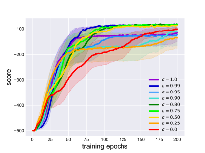
(a) Acrobot-v1

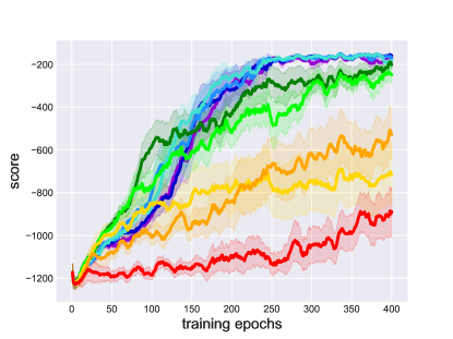
(b) Pendulumn-v0

Figure 1: Learning result in Open AI Gym. $\alpha=1.0$ corresponds to TRPO. Shaded areas denote standard errors.

5 Related Works

The theoretical result and proposed method are extension of the works by Pirotta et al. (2013); Schulman et al. (2015) to on- and off-policy mixture case. Thomas et al. (2015b) proposed an algorithm with monotonic improvement which can use off-policy policy evaluation techique. However, its computational complexity is high. Gu et al. (2017a, b) proposed to interpolate TRPO and deep deterministic policy gradient (Lillicrap et al., 2016), and Gu et al. (2017b) showed the performance bound for their on- and off-policy mixture update as well. In our notation, the penalty terms in their performance bound has $D_{\mathrm{KL}}^{\rm max}(\pi\|\beta)$, which is a constant with respect to the policy after update, $\pi^{\prime}$. In contrast, in Corollary 6, our penalty terms has $D_{\mathrm{KL}}^{\rm max}(\beta\|\pi^{\prime})$ instead of $D_{\mathrm{KL}}^{\rm max}(\pi\|\beta)$, and which is multiplied by $D_{\mathrm{KL}}^{\rm max}(\pi\|\pi^{\prime})$ and $1-\alpha$. Furthermore, our bound is general in the sense that it does not specify how the policy is updatd. Thus all the penalty terms in Eq. (4) can be controlled in a well-designed optimization procedure to find $\pi^{\prime}$.

6 Conclusion and Outlook

In this paper, we showed that the monotonic policy improvement is guaranteed from on- and off-policy mixture samples, by lower bounding the performance difference of two policies. An optimization scheme which applies the derived bound can be regarded as an off-policy natural policy gradient method. In order to support the theoretical result, we provided the TRPO method using the experience replay as the naive application of our bound, and evaluated the performance with various values of mixture coefficient. An important direction is to find a practical algorithm which uses the metric (5) as a constraint. Determining $\alpha$ depending on $\mathbb{E}_{s\sim\rho^{\beta}}\left[D_{\mathrm{KL}}(\beta\|\pi^{\prime})\right]$ is also an interesting future work.

References

• Abbasi-Yadkori et al. (2016) Yasin Abbasi-Yadkori, Peter L. Bartlett, and Stephen J. Wright. A fast and reliable policy improvement algorithm. In In Artificial Intelligence and Statistics, pages 1338–1346, 2016.
• Bagnell and Schneider (2003) J. Andrew Bagnell and Jeff Schneider. Covariant policy search. In International Joint Conference on Artificial Intelligence, pages 1019––1024, 2003.
• Bertsekas (2011) Dimirti P. Bertsekas. Approximate policy iteration: A survey and some new methods. Journal of Control Theory and Applications, 9(3), 2011.
• Degris et al. (2012) Thomas Degris, Martha White, and Richard S. Sutton. Off-policy actor-critic. In International Conference on Machine Learning, 2012.
• Gu et al. (2017a) Shixiang Gu, Timothy Lillicrap, Zoubin Ghahramani, Richard E Turner, and Sergey Levine. Q-prop: Sample-efficient policy gradient with an off-policy critic. In International Conference on Learning Representations, 2017a.
• Gu et al. (2017b) Shixiang Gu, Timothy Lillicrap, Zoubin Ghahramani, Richard E Turner, Bernhard Schölkopf, and Sergey Levine. Interpolated policy gradient: Merging on-policy and off-policy gradient estimation for deep reinforcement learning. In Advances in Neural Information Processing Systems, 2017b.
• Harutyunyan et al. (2016) Anna Harutyunyan, Marc G. Bellemare, Tom Stepleton, and Rémi Munos. Q($\lambda$) with off-policy corrections. In International Conference on Algorithmic Learning Theory, pages 305–320, 2016.
• Haviv and Heyden (1984) Moshe Haviv and Ludo Van Der Heyden. Perturbation bounds for the stationary probabilities of a finite markov chain. Advances in Applied Probability, 16(4), 1984. URL http://www.jstor.org/stable/1427341.
• Kakade (2001) Sham Kakade. A natural policy gradient. In Advances in Neural Information Processing Systems, volume 14, 2001.