Balanced power diagrams for redistricting

Abstract

We explore a method for redistricting, decomposing a geographical area into subareas, called districts, so that the populations of the districts are as close as possible and the districts are compact and contiguous. Each district is the intersection of a polygon with the geographical area. The polygons are convex and the average number of sides per polygon is less than six. The polygons tend to be quite compact. With each polygon is associated a center. The center is the centroid of the locations of the residents associated with the polygon. The algorithm can be viewed as a heuristic for finding centers and a balanced assignment of residents to centers so as to minimize the sum of squared distances of residents to centers; hence the solution can be said to have low dispersion.

1 Introduction

Redistricting.

Redistricting, in the context of elections refers to decomposing a geographical area into subareas such that all subareas have the same population. The subareas are called districts. In most US states, districts are supposed to be contiguous to the extent that is possible. Contiguous can reasonably be interpreted to mean connected.

In most states, districts are also supposed to be compact. This is not precisely defined in law. Some measures of compactness are based on boundaries; a district is preferred if its boundaries are simpler rather than contorted. Some measures are based on dispersion, “the degree to which the district spreads from a central core” [17]. Idaho directs its redistricting commision to “avoid drawing districts that are oddly shaped.” Other states loosely address the meaning of compactness: “Arizona and Colorado focus on contorted boundaries; California, Michigan, and Montana focus on dispersion; and Iowa embraces both” [17].

Balanced centroidal power diagrams

The goal of this paper is to explore a particular approach to redistricting: balanced centroidal power diagrams. Given the locations of a state’s $m$ residents and given the desired number $k$ of districts, a balanced centroidal power diagram partitions the state into $k$ districts with the following desirable properties:

(P1)

each district is the intersection of the state with a convex polygon,

(P2)

the average number of sides per polygon is less than six, and

(P3)

the populations of the districts differ by at most one.

A balanced centroidal power diagram is a particular kind of (not necessarily optimal) solution to an optimization problem called balanced $k$-means clustering: given a set $P$ of $m$ points (the residents) and the desired number $k$ of clusters, a solution (not necessarily of minimum cost) consists of a sequence $C$ of $k$ points (the centers) and an assignment $f$ of residents to centers that is balanced: it assigns $\lfloor m/k\rfloor$ residents to the first $i$ centers, and $\lceil m/k\rceil$ residents to the remaining $k-i$ centers (for the $i$ such that $i\lfloor m/k\rfloor+(k-i)\lceil m/k\rceil=m$). The cost of a solution $(C,f)$ is the sum, over the residents, of the square of the Euclidean distance between the resident’s location and assigned center. (This is a natural measure of dispersion.) In balanced $k$-means clustering, one seeks a solution of minimum cost. This problem is NP-hard [19].

A balanced centroidal power diagram arises from a solution to balanced $k$-means clustering that is not necessarily of minimum cost. Instead, the solution $(C,f)$ only needs to be a local minimum, meaning that it is not possible to lower the cost by just varying $f$ (leaving $C$ fixed), or just varying $C$ (leaving $f$ fixed). Local minima tend to have low cost, so tend to have low dispersion.

Section 2 reviews the meaning of the terms centroidal and power diagram, and discusses how any such local minimum yields districts (with each district containing the residents assigned to one center) for which the desirable properties (P1)–(P3) are mathematically guaranteed. Convex polygons with few sides are arguably well shaped, and their boundaries are arguably not contorted.

The idea and its application to redistricting are not novel. Spann et al. [22] describes a method to find a centroidal power diagram that is nearly balanced (to within 2%). Their solutions are thus not exactly balanced in the sense we have defined. We discuss this and other related work in Section 2.

Figures 1 to 8 show proposed districts corresponding to balanced centroidal power diagrams for the six most populous states in the U.S, based on population data from the 2010 census (locating each resident at the centroid of that resident’s census block). We will also show such diagrams at a web site,  district.cs.brown.edu.

We computed these diagrams efficiently using a variant of Lloyd’s algorithm: start with a random set $C$ of centers, then repeat the following steps until an equilibrium is reached: (1) given the current set $C$ of centers, compute a balanced assignment $f$ that minimizes the cost; (2) given that assignment $f$, change the locations of the centers in $C$ so as to minimize the cost.

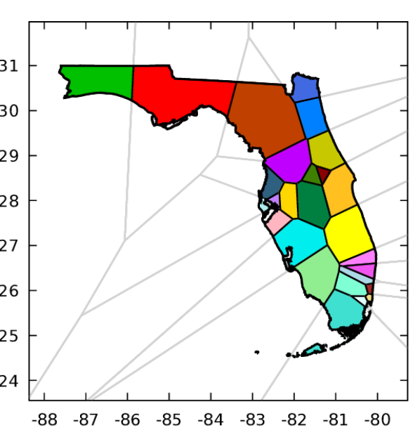
Figure 1: Florida (27 districts)

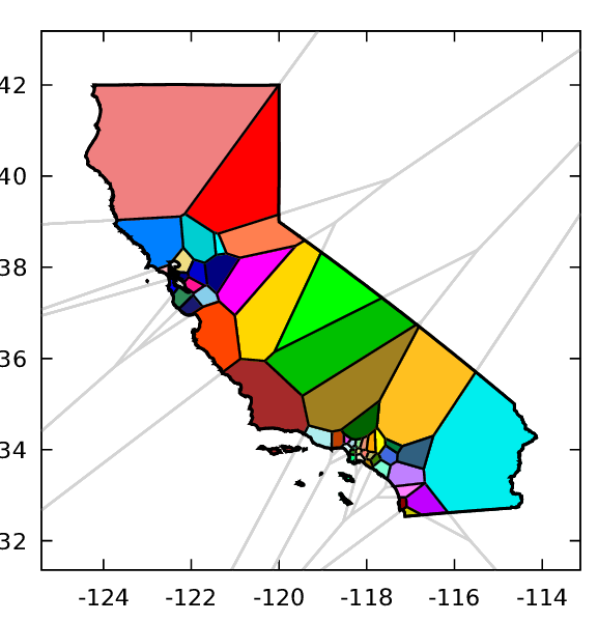
Figure 2: California (53 districts).

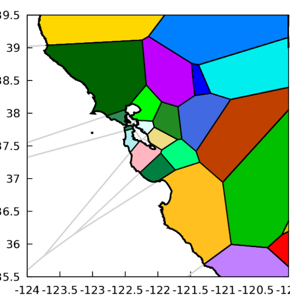
Figure 3: Bay Area (detail of California).

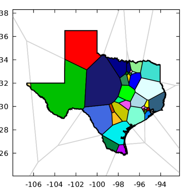
Figure 4: Texas (36 districts).

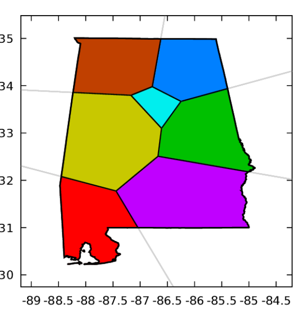
Figure 5: Alabama (7 districts).

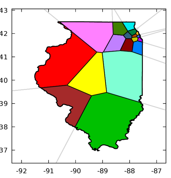
Figure 6: Illinois (18 districts).

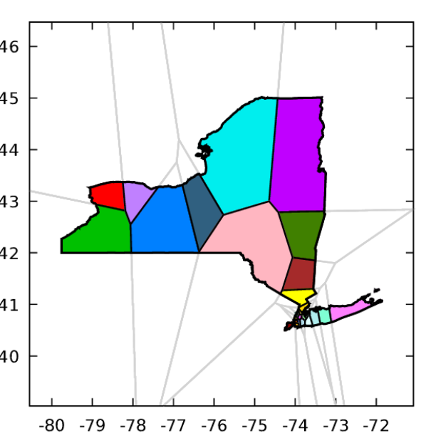
Figure 7: New York (27 districts).

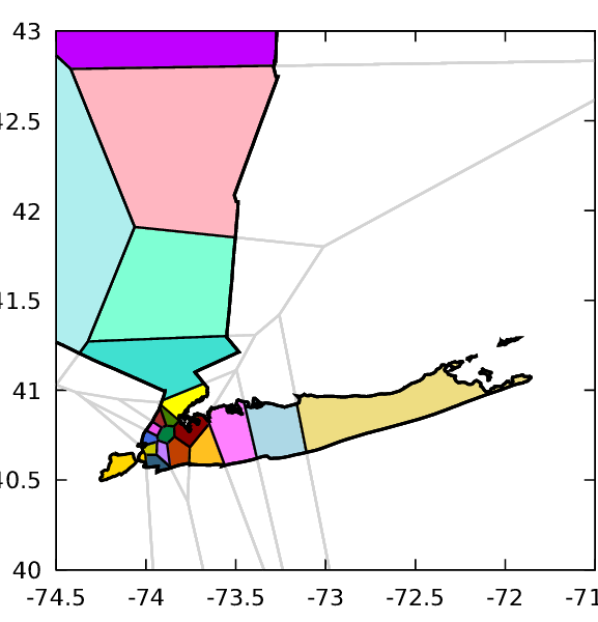
Figure 8: Long Island, New York and Manhattan (detail from New York).

Some might object that the method does not provide the scope for achieving some other goals, e.g. creating competitive districts. A counterargument is that one should avoid providing politically motivated legislators the scope to select boundaries of districts so as to advance political goals. According to this argument, the less freedom to influence the district boundaries, the better. This method does not guarantee fairness in outcome; the fairness is in the process. This point was made, e.g., by Miller [20].

Note that in real applications of redistricting, the locations of people are not given precisely. Rather, there are regions, called census blocks, and each such region’s population is specified.

2 Balanced centroidal power diagrams

The use of optimization, generally, for redistricting has been proposed starting at least as far back as 1965 and has continued up to the present [15, 12, 11]. See [1, 21] for additional references.

In what follows, we focus specifically on the use of balanced centroidal power diagrams. Next is a summary of the relevant history, interspersed with necessary definitions. Throughout, $P$ (the population) denotes a set of $m$ residents (points in a Euclidean space), $C$ denotes a sequence of $k$ centers (points in the same space), $f:P\rightarrow C$ denotes an assignment of residents to centers, and $d(y,x)$ denotes the distance from $y\in P$ to $x\in C$. We generally consider the parameters $P$ and $k$ to be fixed throughout, while $C$ and $f$ vary.

The power diagram of $(C,w)$.

Given any sequence $C$ of centers, and a weight $w_{x}\in\mathbb{R}$ for each center $x\in C$, the power diagram of $(C,w)$, denoted ${\cal P}(C,w)$, is defined as follows. For any center $x\in C$, the weighted squared distance from any point $y$ to $x$ is $d^{2}(y,x)-w_{x}$. The power region $C_{x}$ associated with $x$ consists of all points whose weighted squared distance to $x$ is no more than the weighted squared distance to any other center. The power diagram ${\cal P}(C,w)$ is the collection of these power regions.

An assignment $f:P\rightarrow C$ is consistent with ${\cal P}(C,w)$ if every resident assigned to center $x$ belongs to the corresponding region $C_{x}$. (Residents in the interior of $C_{x}$ are necessarily assigned to $x$.) ${\cal P}(C,w,f)$ denotes the power diagram ${\cal P}(C,w)$ augmented with such an assignment.

Power diagrams are well-studied [3]. If the Euclidean space is $\mathbb{R}^{2}$, it is known that each power region $C_{x}$ is necessarily a (possibly infinite) convex polygon. If each weight $w_{x}$ is zero, the power diagram is also called a Voronoi diagram, and denoted ${\cal V}(C)$. Likewise ${\cal V}(C,f)$ denotes the Voronoi diagram extended with a consistent assignment $f$ (which simply assigns each resident to a nearest center).

Centroidal power diagrams.

A centroidal power diagram is an augmented power diagram ${\cal P}(C,w,f)$ such that the assignment $f$ is centroidal: each center $x\in C$ is the centroid (center of mass) of its assigned residents, $\{y\in P:x=f(y)\}$.

Centroidal Voronoi diagrams.

Centroidal Voronoi diagrams (a special case of centroidal power diagrams) have many applications [10]. One canonical application from graphics is downsampling a given image, by partitioning the image into regions, then selecting a single pixel from each region to represent the region. Centroidal Voronoi diagrams are preferred over arbitrary Voronoi diagrams because the regions in centroidal Voronoi diagrams tend to be more compact.

Lloyd’s method is a standard way to compute a centroidal Voronoi diagram ${\cal V}(C,f)$, given $P$ and the desired number of centers, $k$ [10, § 5.2]. Starting with a sequence $C$ of $k$ randomly chosen centers, the method repeats the following steps until the steps do not cause a change in $f$ or $C$:

1. Given $C$, let $f$ be any assignment assigning each resident to a nearest center in $C$.

2. Move each center $x\in C$ to the centroid of the residents that $f$ assigns to $x$.

Recall that the cost is $\sum_{y\in P}d^{2}(y,f(y))$. Step (1) chooses an $f$ of minimum cost, given $C$. Step (2) moves the centers to minimize the cost, given $f$. Each iteration except the last reduces the cost, so the algorithm terminates and, at termination, $(C,f)$ is a local minimum in the following sense: by just moving centers in $C$, or just changing $f$, it is not possible to reduce the cost.

In the last iteration, Step (1) computes $f$ that is consistent with ${\cal V}(C)$, and Step (2) does not change $C$, so $f$ is centroidal. So, at termination, ${\cal V}(C,f)$ is the desired centroidal Voronoi diagram.

Miller [20] and Kleiner et al. [16] explore the use of centroidal Voronoi diagrams specifically for redistricting. The resulting districts (regions) are guaranteed to be polygonal, and tend to be compact, but their populations can be far from balanced. To address this, consider instead balanced centroidal power diagrams, described next, which can be computed using a capacitated variant of Lloyd’s method.

Balanced power diagrams.

A balanced power diagram is an augmented power diagram ${\cal P}(C,w,f)$ such that the assignment $f$ is balanced (as defined in the introduction). Hence, the numbers of residents in the regions of ${\cal P}(C,w)$ differ by at most 1. Such regions are desirable in many applications.

Aurenhammer et al. [4, Theorem 1] give an algorithm that, in the case of a Euclidean metric, given $P$ and $C$, computes weights $w$ and an assignment $f$ such that ${\cal P}(C,w,f)$ is a balanced power diagram, and $f$ has minimum cost among all balanced assignments of $P$ to $C$. We observe in Section 3.1 that, given $P$, $C$, there exist weights $w$ such that ${\cal P}(C,w,f)$ is a balanced power diagram for any minimum-cost balanced assignment $f$ and any metric. Such an argument was previously presented by Spann et al. [22].

Computing a balanced centroidal power diagram for $P$.

A balanced centroidal power diagram is an augmented power diagram ${\cal P}(C,w,f)$ such that $f$ is both balanced and centroidal. We implement the following capacitated variant of Lloyd’s method to compute such a diagram, given $P$ and the desired number $k$ of centers. Starting with a sequence $C$ of $k$ randomly chosen centers, repeat the following steps until Step (2) doesn’t change $C$:

1. Given $C$, compute a minimum-cost balanced assignment $f:P\rightarrow C$.

2. Move each center $x\in C$ to the centroid of the residents that $f$ assigns to it.

As in the analysis of the uncapacitated method, each iteration except the last reduces the cost, $\sum_{y\in P}d^{2}(y,f(y))$, and at termination, the pair $(C,f)$ is a local minimum in the following sense: by just moving the centers in $C$, or just changing $f$ (while respecting the balance constraint), it is not possible to reduce the cost.

The problem in Step (1) can be solved via Aurenhammer et al.’s algorithm, described previously. Instead, as described in Section 3.1, we solve it by reducing it to minimum-cost flow; yielding both the stipulated $f$ and (via the dual variables) weights $w$ such that ${\cal P}(C,w,f)$ is a balanced power diagram. Note that the solution obtained by minimum-cost flow assigns assigns each person to a single district. In the last iteration, Step (2) does not change $C$, so $f$ is also centroidal, and at termination ${\cal P}(C,w,f)$ is a balanced centroidal power diagram, as desired.

In previous work, Spann et al. [22] proposed a similar iterative method to find a centroidal power diagram. They did not seem to be aware of the work of Aurenhammer [4] but used a duality argument to derive power weights. It is not clear from their paper precisely how their method carries out Step (1). They state that their implementation starts by allowing a 20% deviation from balance, and iteratively reduces the allowed deviation over a series of iterations, adjusting the target populations per district, and terminates when the deviation is within 2% of balanced. We believe that the additional complexity and the failure to achieve perfect balance is a result of the authors’ effort to ensure that census blocks are not split.

Hess et al. [15] had previously given a similar method. Like that of Spann et al., this method ensures that census enumeration districts (analogous to census blocks) were not split, and as a consequence did not achieve perfect balance. Unlike the method of Spann et al., the method of Hess et al. did not compute power weights and did not output a power diagram; presumably each output district is defined as the union of census enumeration districts and is therefore not guaranteed to be connected.

Balzer et al. [5, 6] proposed an algorithm equivalent to the iterative algorithm above, except that a local-exchange heuristic (updating $f$ by swapping pairs of residents) was proposed to carry out Step (1). That heuristic does not guarantee that $f$ has minimum cost (given $C$), so does not in fact guarantee that the assignment is consistent with a balanced power diagram (see Figure 9).

Other previously published algorithms [5, 6, 18, 9, 23] for balanced centroidal power diagrams address applications (e.g. in graphs) that have very large instances, and for which it is not crucial that the power diagrams be exactly centroidal or exactly balanced. This class of algorithms prioritize speed, and none are guaranteed to find a local minimum $(C,f)$, nor a balanced centroidal power diagram.

Helbig, Orr, and Roediger [14] proposed a somewhat similar redistricting algorithm. Like the algorithm above, their algorithm initializes the center locations randomly and then alternates between (1) using mathematical programming to find an assignment of residents to centers and (2) replacing each center with the centroid of the residents assigned to it.

But their assignment of residents to centers is chosen in each iteration to minimize the sum of distances, not the sum of squared distances. This means that the partition does not correspond to a power diagram. Indeed, Helbig et al. acknowledge the possibility that noncontiguous districts could result although they did not observe this occurring.

Their mathematical program for the assignment also treats each “population unit” (e.g. census block) atomically, rather than treating each individual that way. Thus their method never splits a population unit into two districts. While a solution with this property might be desirable, imposing this requirement means that a solution might not exist that achieves population balance. Moreover, their mathematical program constrains the number of population units assigned to a center to be a certain number, rather than constraining the population to be a certain number. Since different population units have different populations, this might not achieve population balance. Helbig et al. address this issue by iteratively modifying the number of population units to be assigned to each center using a heuristic. This does not guarantee convergence, so they allow their algorithm to stop before reaching a true local minimum.

For an excellent survey of the redistricting algorithms, including additional discussion of the Spann et al. algorithm and extensions to districts lying on the sphere, see the online survey by Olson and Smith [21].

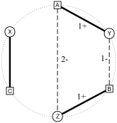
Figure 9: A counter-example to the swap-based balanced assignment algorithm of Balzer et al. [5, 6]. The $k=3$ centers $C=\{A,B,C\}$ (each of capacity 1) are the even vertices of a hexagon with unit sides. The $m=3$ residents $P=\{X,Y,Z\}$ are the odd vertices. The vertices are perturbed slightly so that the edges in $M^{\prime}=\{(A,Y),(B,Z),(C,X)\}$ each have distance slightly more than 1, while the edges in $M^{*}=\{(A,X),(B,Y),(C,Z)\}$ each have distance slightly less than 1, making $M^{*}$ the optimal assignment. But if $M^{\prime}$ is the current assignment, for any two sites, say, $A$ and $B$, there is only one possible swap, and it increases the squared distances (by about $(2^{2}+1^{1})-(1^{2}+1^{1})=3$). So no local improvement is possible from $M^{\prime}$, even though $M^{\prime}$ does not minimize the sum of the squared distances.

3 An Implementation

3.1 Minimum-cost flow

Aurenhammer et al. [4] provide an algorithm that, given the set $P$ of locations of residents and the sequence $C$ of centers, and given a target population for each center (where the targets sum to the total population), finds a minimum-cost assignment $f$ of residents to centers subject to the constraint that the number of residents assigned to each center equals the center’s target population. Their algorithm also outputs weights $w$ for the centers such that the assignment $f$ is consistent with ${\cal P}(C,w)$. Their algorithm can be used to find a minimum-cost balanced assignment by using appropriate targets.

In the implementation here, we take a different approach to computing the minimum-cost balanced assignment: we use an algorithm for minimum-cost flow. Aurenhammer et al. [4] acknowledge that a minimum-cost flow algorithm can be used but argue that their method is more computationally efficient. As we observe below, the necessary weights $w$ can be computed from the values of the variables of the linear-programming dual to minimum-cost flow.

The goal is to find a balanced assignment $f:P\rightarrow C$ of minimum cost, $\sum_{y\in P}d^{2}(y,p(y))$. Let $u_{x}\in\{\lfloor m/k\rfloor,\lceil m/k\rceil\}$ be the number of residents that $f$ must assign to center $x\in C$.

Consider the following linear program and dual:

$\displaystyle\text{minimize}_{a}~{}\hbox to0.0pt{$\displaystyle\textstyle\sum_{y\in P,x\in C}d^{2}(y,x)\,a_{yx}$\hss}$ subject to $\displaystyle\textstyle\sum_{y\in P}a_{yx}$ $\displaystyle{}=\mu_{x}$ $\displaystyle(x\in C)$ $\displaystyle\textstyle\sum_{x\in C}a_{yx}$ $\displaystyle{}=1$ $\displaystyle(y\in P)$ $\displaystyle a_{yx}$ $\displaystyle{}\geq 0$ $\displaystyle(x\in C,y\in P)$

$\displaystyle\text{maximize}_{w,z}~{}\hbox to0.0pt{$\displaystyle\textstyle\sum_{x\in C}\mu_{x}\,w_{x}+\sum_{y\in P}z_{y}$\hss}$ subject to $\displaystyle z_{y}$ $\displaystyle\leq d^{2}(y,x)-w_{x}$ $\displaystyle(x\in C,y\in P)$

This linear program models the standard transshipment problem. As the capacities $\mu_{x}$ are integers with $\sum_{x}\mu_{x}=|P|$, it is well-known that the basic feasible solutions to the linear program are 0/1 solutions ($a_{yx}\in\{0,1\}$), and that the (optimal) solutions $a$ correspond to the (minimum-cost) balanced assignments $f:C\rightarrow P$ such that $a_{yx}=1$ if $f(y)=x$ and $a_{yx}=0$ otherwise. The implementation here solves the linear program and dual by using Goldberg’s minimum-cost flow solver [13] to obtain a minimum-cost balanced assignment $f^{*}$ and an optimal dual solution $(w^{*},z^{*})$. For any minimum-cost balanced assignment $f$ (such as $f^{*}$) the resulting weight vector $w^{*}$ gives a balanced power diagram ${\cal P}(C,w^{*},f)$:

Lemma 1 (see also [22]).

Let $(w^{*},z^{*})$ b any optimal solution to the dual linear program above. Let $f$ be any balanced assignment. Then ${\cal P}(C,w^{*},f)$ is a balanced power diagram if and only if $f$ is a minimum-cost balanced assignment.

Proof.

Let $a$ be the linear-program solution corresponding to $f$.

(If.) Assume that $f$ has minimum cost among balanced assignments. Consider any resident $y\in P$. By complimentary slackness, for $x^{\prime}=f^{*}(y)$, the dual constraint for $(x^{\prime},y)$ is tight, that is, $z^{*}_{y}=d^{2}(y,f(y))-w^{*}_{f(y)}.$ Combining this with the dual constraint for $y$ and any other $x\in C$ gives

$$d^{2}(y,f(y))-w^{*}_{f(y)}\,=\,z^{*}_{y}\,\leq\,d^{2}(y,x)-w^{*}_{x}.$$

That is, from $y$, the weighted squared distance to $f(y)$ is no more than the weighted squared distance to any other center $x\in C$. So, $y$ is in the power region $C_{f(y)}$ of its assigned center $f(y)$. Hence, $f$ is consistent with ${\cal P}(C,w)^{*}$, and ${\cal P}(C,w^{*},f)$ is a balanced power diagram.

(Only if.) Assume that $f$ is consistent with ${\cal P}(C,w^{*})$. That is, the weighted squared distance from $y$ to $f(y)$ is no more than the weighted squared distance to any other center $x\in C$. That is, defining $z^{\prime}_{y}=d^{2}(y,f(y))-w^{*}_{f(y)}$,

$$z^{\prime}_{y}\,=\,d^{2}(y,f(y))-w^{*}_{x}\,\leq\,d^{2}(y,x)-w^{*}_{x}.$$

Thus, $(w^{*},z^{\prime})$ is a feasible dual solution. Furthermore, the complimentary slackness conditions hold for $a$ and $(w^{*},z^{\prime})$. That is, $a_{yz}>0\implies f(y)=x\implies z^{\prime}_{y}=d^{2}(y,x)-w^{*}_{x}$. Hence, $a$ and $(w^{*},z^{\prime})$ are optimal. Since $a$ is optimal, $f$ has minimum cost. ∎

3.2 Experiments

We ran the implementation on various instances of the redistricting problem. We considered the following US states: Alabama, California, Florida, Illinois, New York, and Texas. Note that this list of states contains the biggest states in terms of population and number of representatives, and so our algorithm is usually faster on smaller states.

For each of these states, we used the data provided by the US Census Bureau [8], namely the population and housing unit count by block from the 2010 census. Hence, the input for our algorithm was a weighted set of points in the plane where each point represents a block and its weight represents the number of people living in the block. For each state, we defined the number of clusters to be the number of representatives prescribed for the state. See Table 1 for more details.

State	Number of representatives	Population	Number of iterations to converge
Alabama	7	4779736	28
California	53	37253956	49
Florida	27	18801310	51
Illinois	18	12830632	72
New York	27	19378102	65
Texas	36	25145561	42

Table 1: The states considered in our experiments together with the number of clusters (i.e.: number of representatives) and number of clients (i.e. population of the state).

We note that in all cases the algorithm converged to a local optimum.

3.3 Technical details and implementation

The implementation is available at https://bitbucket.org/pnklein/district. It is written mostly in C++. Our implementation makes use of a slightly adapted version of a min-cost flow implementation, cs2 due to Andrew Goldberg and Boris Cherkassky and described in [13]. The copyright on cs2 is owned by IG Systems, Inc., who grant permission to use for evaluation purposes provided that proper acknowledgments are given. If there is interest, we will write a min-cost flow implementation that is unencumbered.

We also provide Python-3 scripts for reading census-block data, reading state boundary data, finding the boundaries of the power regions, and generating gnuplot files to produce the figures shown in the paper. These figures superimposed the boundaries of the power regions and the boundaries of states (obtained from [7]).

For our experiments, the programs were compiled using g++-7 and run on a laptop with processor Intel Core i7--6600U CPU, 2.60GHz and total virtual memory of 8GB. The system was Debian buster/sid. The total running time was less than fifteen minutes for all instances except California, which took about an hour.

4 Concluding remarks

The method explored in this paper outputs districts that are convex polygons with few sides on average and that are balanced with respect to population, i.e. where the populations in two districts differ by at most one. However, such balance cannot be guaranteed under a requirement that certain geographical regions, e.g. census blocks or counties, remain intact. Since the locations of people within census blocks are not known, the requirement is sensible. One possible way to address the requirement is to first compute districts while disregarding the requirement, then use dynamic programming to modify the solution to obey that requirement while minimizing the resulting imbalance.

We have focused in this paper on the Euclidean plane. This ensures that each district is the intersection of the geographical region (e.g. state) with a polygon. However, in view of the fact that the method explored here might generate a district that includes residents separated by water, mountains, etc., one might want to consider a different metric, e.g. to take travel time into account. Suppose, for example, the metric is that of an undirected graph with edge-lengths. One can use essentially the same algorithm for finding a balanced centroidal power diagram. Computing a minimum-cost balanced assignment (Step 1) and the associated weights can still be done using an algorithm for minimum-cost flow as described in Section 3.1. In Step 2, the algorithm must move each center to the location that minimizes the sum of squared distances from the assigned residents to the new center location. In a graph, we limit the candidate locations to the vertices and possibly locations along the edges. Under such a limit, it is not hard to compute the best locations.

5 Acknowledgements

Thanks to Warren D. Smith for informing us of references [21, 22].

References

- [1] Micah Altman and Michael McDonald. The promise and perils of computers in redistricting. Duke J. Const. L. & Pub. Pol’y, 5:69, 2010.
- [2] David Arthur and Sergei Vassilvitskii. -means++: the advantages of careful seeding. In Proceedings of the Eighteenth Annual ACM-SIAM Symposium on Discrete Algorithms, pages 1027–1035, 2007.
- [3] Franz Aurenhammer. Power diagrams: Properties, algorithms and applications. SIAM Journal on Computing, 16(1):78–96, February 1987.
- [4] Franz Aurenhammer, Friedrich Hoffmann, and Boris Aronov. Minkowski-type theorems and least-squares clustering. Algorithmica, 20(1):61–76, 1998.
- [5] Michael Balzer and Daniel Heck. Capacity-constrained Voronoi diagrams in finite spaces. In Proceedings of the 5th Annual International Symposium on Voronoi Diagrams in Science and Engineering, Kiev, Ukraine, September 2008. 00014.
- [6] Michael Balzer, Thomas Schlömer, and Oliver Deussen. Capacity-constrained point distributions: A variant of Lloyd’s method. Proceedings of ACM SIGGRAPH 2009, 28(3), August 2009.
- [7] United States Census Bureau. Cartographic boundary shapefiles –states. https://www.census.gov/geo/maps-data/data/cbf/cbf_state.html. accessed September 2017.
- [8] United States Census Bureau. Tiger/line with selected demographic and economic data; population % housing unit counts — blocks. https://www.census.gov/geo/maps-data/data/tiger-data.html. accessed September 2017.
- [9] Fernando De Goes, Katherine Breeden, Victor Ostromoukhov, and Mathieu Desbrun. Blue noise through optimal transport. ACM Transactions on Graphics (TOG), 31(6):171, 2012.
- [10] Qiang Du, Vance Faber, and Max Gunzburger. Centroidal Voronoi tessellations: Applications and algorithms. SIAM review, 41(4):637–676, 1999.
- [11] David Eppstein, Michael Goodrich, Doruk Korkmaz, and Nil Mamano. Defining equitable geographic districts in road networks via stable matching. arXiv preprint arXiv:1706.09593, 2017.
- [12] R. S. Garfinkel and G. L. Nemhauser. Optimal political districting by implicit enumeration techniques. Management Science, 16(8):B–495, April 1970.
- [13] Andrew V. Goldberg. An efficient implementation of a scaling minimum-cost flow algorithm. J. Algorithms, 22(1):1–29, 1997.
- [14] Robert E Helbig, Patrick K Orr, and Robert R Roediger. Political redistricting by computer. Communications of the ACM, 15(8):735–741, 1972.
- [15] S. W. Hess, J. B. Weaver, H. J. Siegfeldt, J. N. Whelan, and P. A. Zitlau. Nonpartisan political redistricting by computer. Operations Research, 13(6):998–1006, 1965.
- [16] Evan Kleiner and Albert Schueller. A political redistricting tool for the rest of us — other approaches to redistricting. Convergence (MAA), November 2013.
- [17] Justin Levitt. All about redistricting: Professor justin levitt’s guide to drawing the electoral lines. http://redistricting.lls.edu/. accessed September 2017.
- [18] Hongwei Li, Diego Nehab, Li-Yi Wei, Pedro V. Sander, and Chi-Wing Fu. Fast capacity constrained Voronoi tessellation. In Proceedings of the 2010 ACM SIGGRAPH Symposium on Interactive 3D Graphics and Games, I3D ’10, pages 13:1–13:1, New York, NY, USA, 2010. ACM.
- [19] Meena Mahajan, Prajakta Nimbhorkar, and Kasturi Varadarajan. The planar -means problem is NP-hard. In International Workshop on Algorithms and Computation, pages 274–285. Springer, 2009.
- [20] Stacy Miller. The problem of redistricting: The use of centroidal Voronoi diagrams to build unbiased congressional districts. Senior project, Whitman College, 2007.
- [21] Brian Olson and Warren D. Smith. RangeVoting.org - Theoretical Issues in Districting Algorithms. http://rangevoting.org/TheorDistrict.html, accessed 2017-12-08.
- [22] Andrew Spann, Daniel Kane, and Dan Gulotta. Electoral redistricting with moment of inertia and diminishing halves models. The UMAP Journal, 28(3):281–299, 2007.
- [23] Shi-Qing Xin, Bruno Lévy, Zhonggui Chen, Lei Chu, Yaohui Yu, Changhe Tu, and Wenping Wang. Centroidal power diagrams with capacity constraints: Computation, applications, and extension. ACM Transactions on Graphics, 35(6):1–12, November 2016.