SISSO: a compressed-sensing method for identifying the best low-dimensional descriptor in an immensity of offered candidates

Abstract

The lack of reliable methods for identifying descriptors — the sets of parameters capturing the underlying mechanisms of a materials property — is one of the key factors hindering efficient materials development. Here, we propose a systematic approach for discovering descriptors for materials properties, within the framework of compressed-sensing based dimensionality reduction. SISSO (sure independence screening and sparsifying operator) tackles immense and correlated features spaces, and converges to the optimal solution from a combination of features relevant to the materials’ property of interest. In addition, SISSO gives stable results also with small training sets. The methodology is benchmarked with the quantitative prediction of the ground-state enthalpies of octet binary materials (using ab initio data) and applied to the showcase example of predicting the metal/insulator classification of binaries (with experimental data). Accurate, predictive models are found in both cases. For the metal-insulator classification model, the predictive capability are tested beyond the training data: It rediscovers the available pressure-induced insulator$\rightarrow$metal transitions and it allows for the prediction of yet unknown transition candidates, ripe for experimental validation. As a step forward with respect to previous model-identification methods, SISSO can become an effective tool for automatic materials development.

Introduction

The materials-genome initiative MGI_OSTP_new has fostered high-throughput calculations and experiments. Correspondingly, computational initiatives (e.g., Refs. aflow ; materialsproject.org ; oqmd.org ; cmr_repository ), have already tackled many thousands of different systems (see White2013 ; Luca2015 ; Kalidindi2015 ; Ceder_BigData_SA2016 ; curtarolo:art112 ; Wolverton_ML_NPJ2016 ; curtarolo:art124 ; Tanaka_ML ; curtarolo:art81 ; MeredigICSD_NMAT2013 ; Fischer06 ). Much of the data of this field is available in the FAIR Repository and Archive of the NOMAD Center of Excellencenomad-coe.eu ; NOMAD_MRS . On close inspection, one realizes that such data collections are so-far inefficiently exploited, and only a tiny amount of the contained information is actually used. Despite the number of possible materials being infinite, the request for specific properties — e.g.,“a material that is stable, non-toxic, with an optical band gap between 0.8 and 3.2 eV” — drastically reduces the set of candidates. This implies that, in terms of functional materials, the structural and chemical space of compounds is sparsely populated. Identifying these few materials — known materials as well as materials that have not been created to date — requires an accurate, predictive approach.

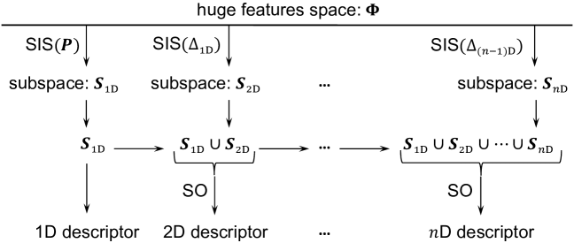
Figure 1: The method SISSO combines unified subspaces having the largest correlation with residual errors $\bm{\Delta}$ (or $\bm{P}$) generated by SIS (sure independence screening) with SO (sparsifying operator) to further extract the best descriptor.

Several methods, falling under the umbrella names of artificial intelligence or (big-)data analytics (including data mining, machine/statistical learning, compressed sensing, etc.) have being developed and applied to the wealth of materials-science data Bartok_PRL_2010 ; curtarolo:art85 ; Rajan_AnnRev2015 ; Mueller_MLMS_2016_review ; Kim_ChemMat_2016 ; Lilienfeld2016 ; Takahashi_DalTrans2016 ; Ceriotti2017 ; Goldsmith_NJP_2017 ; Pham_jcp2018 , but so far, no general and systematic approach has been established and demonstrated. The challenge here is that many different processes and phenomena exist, controlled by atomic structure, electron charge, spin, phonons, polarons and other quasiparticles, and tiny changes in structure or composition can cause a qualitative change of the materials property (phase transitions). For example, less than 0.001% impurities can turn an insulator into a conductor. This type of complexity is a significant element of ‘the fourth paradigm in materials science’ Hey_Forth_Paradigm_Book_Microsoft ; Agrawal_APLM_2016 ; NOMAD_MRS which recognizes that it may not be possible to describe many properties of functional materials by a single, physically founded model, i.e., via a closed, analytical expression. The reason is that such properties are determined by several multi-level, intricate theoretical concepts. Thus, insight is obtained by searching for structure and patterns in the data, which arise from functional relationships (including but not limited to linear correlations) with different processes and functions. Finding a descriptor — the set of parameters capturing the underlying mechanism of a given materials property or function — that reveals these relationships is the key, intelligent step. Once the descriptor has been identified, essentially every learning approach (e.g., regressions — including kernel-based ones —, artificial neural networks, etc.) can be applied straightforwardly. These issues and in particular the central role of the descriptor was implicitly assumed in many seminal machine-learning works applied to materials science, but it was only later explicitly identified in the works of Ghiringhelli et al. Luca2015 ; Luca2017 . These authors recast the descriptor-search challenge into a compressed-sensing (CS) formulation. The CS approach has been shown to be effective for reproducing a high quality “reconstructed signal” starting from a very small set of “observations” CandesWakin_IEEE_SPM_2008 ; Nelson2013 . Mathematically, given a set of samples measured incoherently, $\bm{P}$, CS finds the sparse solution $\bm{c}$ of an underdetermined system of linear equations $\bm{D}\bm{c}=\bm{P}$ ($\bm{D}$ is called the sensing matrix with columns $\gg$ rows). If the number of nonzero entries in $\bm{c}$ is smaller than the size of $\bm{P}$, then CS effectively reduces the dimensionality of the problem CandesRombergTao_IEEE_TIT_2006 ; Donoho2006 ; CandesWakin_IEEE_SPM_2008 . In the specific case treated in Luca2015 ; Luca2017 , given a set of materials $m_{i}$ with observable properties listed in vector $\bm{P}_{i}$ and a huge list of possible test features $d_{j}$ (forming the features space), the linear projection of each $i$-material into the $j$-feature forms the $i,j$ components of the sensing matrix $\bm{D}$. The sparse solution of “$\operatorname*{arg\,min}_{\bm{c}}\left(\lVert\bm{P}-\bm{Dc}\rVert^{2}_{2}+\lambda\lVert{\bm{c}}\rVert_{0}\right)$”, where $\lVert{\bm{c}}\rVert_{0}$ is the number of nonzero components of $\bm{c}$, gives the optimum $n$-dimensional descriptor, i.e., the set of features “selected” by the the $n$ non-zero components of the solution vector $\bm{c}$.

In Refs. Luca2015 ; Luca2017 , a modification of LASSO (least absolute shrinkage and selection operator, LASSO ) was introduced for finding the optimal solution. However, moving beyond the showcase application demonstrated in those papers (predicting the ground-state crystal structure of octet binaries semiconductors), it turns out that the method is unable to deal with large feature spaces, i.e. with situations where knowledge about the underlying processes is not well developed and when in addition to the atomic properties, also collective properties, e.g. the electronic band structure, play a role. When the space of candidate descriptors (the feature space) gets large (larger than few thousands elements) and/or when features are correlated, the approach breaks down.

In the present paper, we provide a strong and efficient solution of these problems, i.e. we present a new method, called SISSO (sure independent screening and sparsifying operator), which can deal with an immensity of offered candidate descriptors (billions, or more) and does not suffer when features are correlated. The outcome of SISSO is a mathematical model, in the form of explicit, analytic functions of basic, input physical quantities. This aspect gives the opportunity to inspect the equations and suggest means to test the generalization ability of the model.

Results and Discussion

Features e space construction. All quantities that are hypothesized to be relevant for describing the target property (the so called primary features Luca2015 ; Luca2017 ) are used as starting point for the construction of the space Sondhi2009 ; Guyon2003 . Features are of atomic (species per se) and collective origin (atoms embedded in the environment). Then, a combination of algebraic/functional operations is recursively performed for extending the space. For instance, the starting point $\bm{\Phi}_{0}$ may comprise readily available and relevant properties, such as atomic radii, ionization energies, valences, bond distances and so on. The operators set is defined as

$$\bm{\hat{H}}^{\rm(m)}\equiv\left\{I,+,-,\times,/,{\rm exp},{\rm log},|-|,\sqrt{\ },^{-1},^{2},^{3}\right\}\left[\phi_{1},\phi_{2}\right],\vspace{-1mm}$$

where $\phi_{1}$ and $\phi_{2}$ are objects in $\Phi$ (for unary operators only $\phi_{1}$ is considered) and the superscript ^(m) indicates that dimensional analysis is performed to retain only “meaningful” combinations (e.g., no unphysical items like ‘size$\,+\,$energy’ or ‘size$\,+\,$size²’). The intrinsically linear relationship observables $\leftrightarrow$ descriptor in the CS formalism is made non-linear by equipping the features space with non-linear operators in $\bm{\hat{H}}^{\rm(m)}$. At each iteration, $\bm{\hat{H}}^{\rm(m)}$ operates on all available combinations, and the features space grows recursively as:

$$\bm{\Phi}_{n}\equiv\bigcup_{i=1}^{n}\bm{\hat{H}}^{\rm(m)}\left[\phi_{1},\phi_{2}\right],\quad\forall\phi_{1},\phi_{2}\in\Phi_{i-1}.\vspace{-2mm}$$ (1)

The number of elements in $\bm{\Phi}_{n}$ grows very rapidly with $n$. It is roughly of the order of $\sim(\#\bm{\Phi}_{0})^{2^{n}}\!\times(\#\bm{\hat{H}_{2}})^{2^{n}-1}$ where $\#\bm{\Phi}_{0}$ and $\#\bm{\hat{H}_{2}}$ are the numbers of elements and binary operators in $\bm{\Phi}_{0}$ and $\bm{\hat{H}}$, respectively. For example, $\#\bm{\Phi}_{3}\sim 10^{11}$ with $\#\bm{\hat{H}_{2}}=5$ and $\#\bm{\Phi}_{0}=10$. To avoid a priori bias and contrary to previous works Sondhi2009 , no features were disregarded despite the size of the resulting features space. Instead, we extend the sparse-solution algorithm (using sparsifying operators (SO) Breen2009 ) and tackle huge sensing matrices representative of features spaces containing coherent elements overcoming the limitations of LASSO based methods Luca2015 ; Luca2017 .

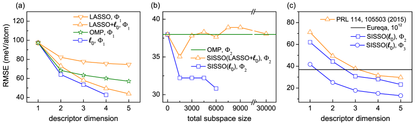
Figure 2: Benchmark of algorithms. (a) Training error: RMSE  versus descriptor dimension for different SOs operating on the smallest $\bm{\Phi}_{1}$. (b) Training error: RMSE versus subspace size in the SIS step to find a 3D descriptor by OMP or SISSO with the same large features space $\bm{\Phi}_{2}$ (a similar picture for a 2D descriptor is presented in the Supplementary Materials). (c) Training error: RMSE by SISSO($\ell_{0}$) with $\bm{\Phi}_{2}$ and $\bm{\Phi}_{3}$ compared with previous work Luca2015 (features space size $\sim 4\,500$) and with the Eureqa software Schmidt2009 (evaluated functions $10^{12}$, larger than $\#\bm{\Phi}_{3}$).

Solution algorithm. The $\ell_{0}$-norm regularized minimization SISSOnoteELLE0 is the obvious path for finding the best sparse solution of linear equations. It is performed through combinatorial optimization by penalizing the number of non-zero coefficients. The algorithm is NP-hard and thus infeasible when the features space becomes very large. Efficient methods can be employed to approximate the correct $\ell_{0}$ solution Donoho2003 with ideal features space (e.g., having uncorrelated basis sets). Amongst them are the convex optimization by $\ell_{1}$-norm SISSOnoteELLE1 regularization LASSO LASSO ) and the various greedy algorithms such as the matching pursuit (MP) MP and orthogonal matching pursuit (OMP) OMP ; Tropp2007 . Unfortunately, with correlated features spaces, approximated results can largely deviate from the ideal $\ell_{0}$ solutions Donoho2003 ; Tropp2004 . Corrections have been proposed, for example the LASSO+$\ell_{0}$ scheme comprising LASSO prescreening and subsequent $\ell_{0}$ optimization Luca2015 ; Luca2017 , and the the $\ell_{1}$-analysis and $\ell_{1}$-synthesis l1-analysis . However, when the features space size becomes of the order of $10^{6}-10^{9}$, $\ell_{1}$ based methods also become computationally infeasible. As previously mentioned, here we overcome the huge size of the problem by combining SO with sure independence screening (SIS) SIS1 ; SIS2 , which has been shown to be effective for dimensionality reduction of ultra-high dimensional features spaces SIS1 . SIS scores each feature (standardized) with a metric (correlation magnitude, i.e., the absolute of inner product between the target property and a feature) and keeps only the top ranked SIS1 . After the reduction, SO is used to pinpoint the optimal $n$-dimensional descriptor. The smaller the dimensionality, the better the outcome: progressively larger $n$ are tested until the “left-over” residual error is within quality expectation. The combination of SIS and SO is called SISSO. Figure 1 illustrates the idea.

SISSO. Out of the huge features space ($\sim 10^{10}$ elements or more), SIS selects the subspace $\bm{S}_{\begin{subarray}{c}\scalebox{0.6}{1D}\end{subarray}}$ containing the features having the largest correlation with the response $\bm{P}$ (target material property). Generally, the larger the subspace $\cup\bm{S}_{\begin{subarray}{c}\scalebox{0.6}{iD}\end{subarray}}$, the higher the probability it contains the optimal descriptor. However, the chosen size of $\cup\bm{S}_{\begin{subarray}{c}\scalebox{0.6}{iD}\end{subarray}}$, depends on i) which type of SO is later used, ii) the dimensionality $n$ requested, and iii) the available computational resources. With SO(LASSO), $\cup\bm{S}_{\begin{subarray}{c}\scalebox{0.6}{iD}\end{subarray}}$ can contain as much as $10^{5}\sim 10^{6}$ elements, depending on $\#\bm{P}$. With SO($\ell_{0}$), the largest obtainable size is typically $10^{5}$ for $n=2$, $10^{3}$ for $n=3$, $10^{2}$ for $n=4$, etc. (because the number of needed evaluation grows combinatorially with $n$). If $n$ is large, e.g., $>$10, then the maximum possible $\#\bm{S}_{\begin{subarray}{c}\scalebox{0.6}{iD}\end{subarray}}$ converge to 1: SISSO becomes OMP. From inside $\bm{S}_{\begin{subarray}{c}\scalebox{0.6}{1D}\end{subarray}}$, SO($\ell_{0}$) finds the best 1D descriptor, which is trivially the first ranked feature. In other words, the SIS solution in 1D is already the SISSO solution. The residual error for a $n$-dimensional model is defined as $\bm{\Delta}_{\begin{subarray}{c}\scalebox{0.6}{nD}\end{subarray}}\equiv\bm{P}-\bm{d}_{\begin{subarray}{c}\scalebox{0.6}{nD}\end{subarray}}\bm{c}_{\begin{subarray}{c}\scalebox{0.6}{nD}\end{subarray}},$ where $\bm{d}_{\begin{subarray}{c}\scalebox{0.6}{nD}\end{subarray}}$ is the matrix with columns being the selected features from the whole features space, and the $\bm{c}_{\begin{subarray}{c}\scalebox{0.6}{nD}\end{subarray}}=({\bm{d}_{\begin{subarray}{c}\scalebox{0.6}{nD}\end{subarray}}}^{T}\bm{d}_{\begin{subarray}{c}\scalebox{0.6}{nD}\end{subarray}})^{-1}{\bm{d}_{\begin{subarray}{c}\scalebox{0.6}{nD}\end{subarray}}}^{T}\bm{P}$ is the least square solution of fitting $\bm{d}_{\begin{subarray}{c}\scalebox{0.6}{nD}\end{subarray}}$ to $\bm{P}$. If the error, the root-mean-square of the residual $\rho_{\begin{subarray}{c}\scalebox{0.6}{RMS}\end{subarray}}(\bm{\Delta}_{\begin{subarray}{c}\scalebox{0.6}{nD}\end{subarray}})$, is below a certain threshold then descriptor is considered fit. Otherwise the method recursively considers a higher dimensional solution. In general, for a $n$-dimensional descriptor, SIS selects the subspace $\bm{S}_{\begin{subarray}{c}\scalebox{0.6}{nD}\end{subarray}}$ with response $\bm{\Delta}_{\begin{subarray}{c}\scalebox{0.6}{(n-1)D}\end{subarray}}$. Then SO extracts the best $n$D descriptor, with response $\bm{P}$, from the union of all the previously selected subspaces $\bm{S}_{\begin{subarray}{c}\scalebox{0.6}{nD}\end{subarray}}\cup\bm{S}_{\begin{subarray}{c}\scalebox{0.6}{(n-1)D}\end{subarray}}\cup\cdots\cup\bm{S}_{\begin{subarray}{c}\scalebox{0.6}{1D}\end{subarray}}$. Candès and Romberg CandesRomberg_InvProb_2007 have shown that to identify the best $n$-dimensional descriptor with “overwhelming probability” the size of the response — in our case the number of materials observations $\bm{P}$ — needs to satisfy the relationship $\#\bm{P}\geq k\cdot n\cdot{\rm log}(\#\Phi)$, where $k$ is a constant (around $1\sim 10$ Luca2017 ) and $\#\Phi$ is the size of the features space CandesWakin_IEEE_SPM_2008 . Differently from the typical CS scenario, here $\#\bm{P}$ is fixed Luca2017 ; then, when $\#\Phi$ increases, the maximum $n$ decreases in order to satisfy the relationship CandesRomberg_InvProb_2007 . In practice, features spaces of growing sizes ($\Phi_{0},\Phi_{i},\cdots$) and different $n$ are tested until a model with required accuracy ($\rho_{\begin{subarray}{c}\scalebox{0.6}{RMS}\end{subarray}}(\bm{\Delta}_{\begin{subarray}{c}\scalebox{0.6}{nD}\end{subarray}})<$ threshold) is obtained.

SISSO has advantages over MP MP and OMP OMP . MP searches a linear model reproducing $\bm{P}$ by adding dimensionality to a descriptor while preserving selected features and corresponding coefficients. OMP improves MP by reoptimizing the coefficients every time a new component is introduced, $n\rightarrow{n+1}$, but still preserving previously selected features. SISSO both reselects features and reoptimizes coefficients at each dimensional increment. SISSO reduces to OMP when each subspace in the union has unit size ($\#\bm{S}_{\begin{subarray}{c}\scalebox{0.6}{iD}\end{subarray}}=1,\forall i$). Still, it differs from iterative SIS SIS1 which reduces to simple MP when all $\#\bm{S}_{\begin{subarray}{c}\scalebox{0.6}{iD}\end{subarray}}=1$.

Benchmark: Quantitative prediction. SISSO is benchmarked by comparing the relative stability of octet binary materials between rock-salt (RS) and zinc-blende (ZB) configurations. The reference data is taken from Ref. Luca2015 , including the target calculated ab initio enthalpy difference, RS and ZB for 82 materials and the 23 primary features related to material compositions forming $\Phi_{0}$. The primary features considered in this study are listed in the Supplementary Materials. All quantities are calculated with density-functional theory in the local-density approximation. Details are given in Refs. Luca2015 ; Luca2017 . Then, with a combination of the previously defined operator set, $\bm{\hat{H}}^{\rm(m)}$, and Eq. (1), the features spaces $\bm{\Phi}_{1}$ (small, $\#\bm{\Phi}_{1}=556$), $\bm{\Phi}_{2}$ (large, $\#\bm{\Phi}_{2}\!\sim\!10^{5}$), and $\bm{\Phi}_{3}$ (huge, $\#\bm{\Phi}_{3}\!\sim 10^{11}$) are constructed.

Figure 2(a). The training errors ($\rho_{\begin{subarray}{c}\scalebox{0.6}{RMS}\end{subarray}}$) of different SO: LASSO, LASSO+$\ell_{0}$, OMP, and $\ell_{0}$ are compared while operating on the small features space $\bm{\Phi}_{1}$. LASSO suffers because of the correlations existing inside $\bm{\Phi}_{1}$ (Figure S1 in the Supplementary Materials); LASSO+$\ell_{0}$ and OMP both surpass LASSO; $\ell_{0}$ is the reference: it gives the exact global minimum solution for descriptors of any dimension. However, even with $\ell_{0}$ the error is still too large for many thermodynamical predictions — $\rho_{\begin{subarray}{c}\scalebox{0.6}{RMS}\end{subarray}}(\bm{\Delta}_{\begin{subarray}{c}\scalebox{0.6}{nD}\end{subarray}})\gtrsim 40$ meV/atom — and this is due to the too-small size of $\bm{\Phi}_{1}$.
Figure 2(b). For the larger $\bm{\Phi}_{2}$, SIS combined with LASSO+$\ell_{0}$ as SO — SISSO(LASSO+$\ell_{0}$) —, SISSO($\ell_{0}$), and OMP are compared for generating a 3D descriptor: SISSO($\ell_{0}$) is the only approach improving consistently with subspace size $\#\!\cup\!\bm{S}_{\begin{subarray}{c}\scalebox{0.6}{iD}\end{subarray}}$ and it always surpasses OMP when each $\#\!\bm{S}_{\begin{subarray}{c}\scalebox{0.6}{iD}\end{subarray}}\!\gg\!1$; SISSO(LASSO+$\ell_{0}$) does not improve over OMP because of the failure of LASSO in dealing with correlated features Donoho2003 . Obviously, the larger the features space and the better the obtainable model (at least equal). When exhaustive searches become computationally impossible, SISSO can still find the optimal solution if the subspace produced by SIS is big enough.
Figure 2(c). The errors for 1- to 5-dimensional descriptors are calculated by SISSO($\ell_{0}$) while operating in the large $\bm{\Phi}_{2}$ and huge $\bm{\Phi}_{3}$ spaces. For $n=1$, SIS reduces to the best 1D descriptor, so no $\ell_{0}$ is needed. For $n=2,3,4,5$ the size of the SIS subspace is chosen to follow the previously mentioned relationship CandesRomberg_InvProb_2007 applied to the subspace $\#\bm{S}\sim{\rm exp}(\#\bm{P}/kn)$. With $\#\bm{P}=82$ and $k=3.125$, the total size of all the selected subspaces is $\#\cup\bm{S}_{\begin{subarray}{c}\scalebox{0.6}{iD}\end{subarray}}=5\cdot 10^{5},6\cdot 10^{3},7\cdot 10^{2},2\cdot 10^{2}$ for $n=2,3,4,5$, respectively. For all these sizes, the application of $\ell_{0}$ regularization as SO involves $10^{10}$–$10^{11}$ independent least-square-regression evaluations. This is computationally feasible due to our (trivially) parallel implementation of SISSO (for instance, for this application, the production calculations were run on 64 cores). The training errors for the descriptors identified from $\bm{\Phi}_{3}$ are systematically better than those coming from $\bm{\Phi}_{2}$, thanks to the higher complexity (functional forms of the descriptors are reported in Supplementary Materials). SISSO($\ell_{0}$) with $\bm{\Phi}_{2}$ is systematically better than the previous work by Ghiringhelli et al. Luca2015 ; Luca2017 , due to the allowed larger features spaces. Note that when SISSO($\ell_{0}$) is applied to the same features space as in Ref. Luca2015 , it also finds the same descriptor: SISSO combined with the features space of Ref. Luca2015, has the same results of the yellow line of Figure 2(c). Performance is also compared with the commercial software Eureqa Schmidt2009 by using the same operator set and primary features ($\bm{\Phi}_{0}$), and $10^{12}$ evaluated functions, a number comparable to $\#\bm{\Phi}_{3}$. SISSO($\ell_{0}$) in $\bm{\Phi}_{3}$ with $n\geq 2$ and SISSO($\ell_{0}$) in $\bm{\Phi}_{2}$ with $n\geq 3$ have both lower training error than Eureqa (see Supplementary Materials).

Figure 3: Benchmark of algorithms. (a) Cross validation: LTOCV and LOOCV results for the features space $\Phi_{3}$ with OMP and SISSO($\ell_{0}$). (b) Cross validation: Box plots of the absolute errors for the SISSO($\ell_{0}$)-LTOCV results with features space $\Phi_{3}$. The upper and lower limits of the rectangles mark the 75% and 25% percentiles of the distribution, the internal horizontal line indicates the median (50% percentile), and the upper and lower limits of the “error bars” depict the 99% and 1% percentiles. The crosses represent the maximum absolute errors.

Figure 3(a). Training errors were illustrated in Figure 2(a-c), in order to directly compare over the same dataset, the ability of different approaches to find optimal or close-to-optimal solutions of the CS problem. With practical applications in mind, it is imperative to determine the performance of the obtained model on data that are not used for the training. In statistical learning Hastie2008 ; Pearl_Book_Inference , this is performed via cross validation (CV), a class of techniques that, by splitting the dataset into a training and a test set in various ways, aims at detecting “underfitting” and “overfitting”, i.e., when the complexity of the fitted model is too small or too large, respectively. In CS, dedicated CV techniques have been proposed Boufounos_CompressSensing_2007 ; Ward_CompressSensing_2008 . Specifically, in a CS-based iterative technique like SISSO, the only source of overfitting can come from a too large dimensionality of the descriptor (note that there is only one fitting coefficient per dimension, i.e., features recursively built via Eq. 1 do not contain fitting parameters). For this benchmark application, we applied the CS-CV scheme proposed in Ref. Boufounos_CompressSensing_2007 with leave-10%-out (LTO) CV (the dataset is split in 40 training set containing 90% randomly selected data points and a test set with the remaining 10%) and leave-one-out (LOO) CV (one data points constitutes the test set, and the procedure is iterated $\#P$ times). The model is trained on the training set (the whole SISSO procedure, i.e., including the selection of the descriptor) and the error is measured on the test set. In such framework, the CV error decreases with the number of iterations — the dimensionality — until the approximate descriptor will try to fit the data (containing possible errors) starting from primary features having intrinsic limitations, thus causing a subsequent increase in the CV error. The iteration at which the CV error starts increasing identifies the maximum dimensionality of that particular model. This is determined by the features space — in turns determined by set of primary features, operators set, and number of iterations of the features space construction — and the training set. CS-CV is performed for $\Phi_{3}$ with the subspace sizes reported in the description of Figure 2(c), and for subspace of unit size (for which SISSO becomes OMP). It is found that the dimensionality minimizing the error is two for both the CV schemes of SISSO($\ell_{0}$). In order to achieve a smaller prediction error, one would then need to add new primary features, possibly substituting features that are never selected in a descriptor, or increase the complexity of the features space, or both. OMP finds the same dimensionality of the problem (2$\sim$3), has a lower computational cost but a cost of worse performance in terms of prediction error.
Figure 3(b) depicts the box plots for the distribution of errors as function of the dimensionality for SISSO($\ell_{0}$)-LTOCV results with features space $\Phi_{3}$ (RMSE shown in (a)). The 1% and 99% (extrema of the “error bar”), the 25% and 75% (lower and upper limits of the rectangle) and the median (intermediate horizontal line) percentiles are marked. The maximum absolute errors are also indicated by crosses. The worsening of the RMSE beyond 2D is mainly determined by an increase in the largest errors (the 99%-percentile), while most of the errors remain small (median/lower percentiles $\sim$ constant).
LOOCV is also used to inspected how often the same descriptor is selected. The test operates in $\#\Phi_{3}$ with SISSO($\ell_{0}$). The LOOCV descriptor agrees with the one found over all data 79, 73, 58 times out of 82 iterations. It is remarkable, as the size of $\Phi_{3}$ is of the order $10^{11}$ features and there are only 82 data points. This means that the 1D, 2D, 3D descriptor is selected from $10^{11}$, $10^{22}$, $10^{32}$ combinations, respectively. We note that descriptors that are selected using the reduced training data set need be correlated with the full data-set descriptors, implying the existence of a “hidden” correlation between the functional forms. Hence, selecting different descriptors does not imply over-fitting (this is independently determined via CS-CV), but choosing different existing approximate functional relationship among the primary features.

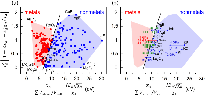
Figure 4: SISSO for classification. (a) An almost perfect classification (99.0%) of metal/nonmetal for 299 materials. Symbols: $\chi$ Pauling electronegativity, $I\!E$ ionization energy, $x$ atomic composition, $\sum V_{\rm atom}/V_{\rm cell}$ packing factor. Red circles, blue squares, and open blue squares represent metals, non-metals, and the three erroneously characterized non-metals, respectively. (c) Reproduction of pressure induced insulator$\rightarrow$metals transitions (red arrows), of materials that remain insulators upon compression (blue arrows), and computational predictions at step of 1GPa (green bars).

Application: classification models. The SISSO framework can be readily adapted to predict categorical properties (as opposed to continuous properties like an energy difference), i.e., it can be applied for classification. In the space of descriptors, each category’s domain is approximated as the region of space (area, in 2D) within the convex hull of the corresponding training data. SISSO finds the low-dimensional descriptor yielding the minimum overlap (or maximum separation) between convex regions. Formally, given a property with $M$ categories, the norm for classification is defined as:

$$\bm{\hat{c}}\equiv\operatorname*{arg\,min}_{\bm{c}}\left(\sum_{i=1}^{M-1}\sum_{j=i+1}^{M}O_{ij}+\lambda\lVert{\bm{c}}\rVert_{0}\right),$$ (2)

where $O_{ij}$ is the number of data in the overlap-region between the $i-$ and $j-$domain, $\bm{c}$ is a sparse vector (0/1 elements) so that a feature $k$ is selected(deselected) when $c_{k}=1(0)$, and $\lambda$ is a parameter controlling the number of nonzero elements in $\bm{c}$. Of all the possible solutions of Eq. (2) having the same dimension and overlap, we chose the one with minimum $n$-dimensional overlap volume Bialon2016 :

$$\Omega\equiv\frac{2}{M(M-1)}\sum_{i=1}^{M-1}\sum_{j=i+1}^{M}\frac{\Omega_{ij}}{\min(\Omega_{i},\Omega_{j})},$$ (3)

where $\Omega_{i}$, $\Omega_{j}$, and $\Omega_{ij}$ are the $n$-dimensional volumes of the $i-$, $j-$, and overlap $ij-$domains. Finally, the SIS correlation “property$\leftrightarrow$feature” is defined as $\left(\sum_{i=1}^{M-1}\sum_{j=i+1}^{M}O_{ij}+1\right)^{-1}$: high correlation $\Leftrightarrow$ low overlap.

SISSO for classification is tested on a simple metal/nonmetal classification of binary systems. The training systems are far from creating an exhaustive list and, as such, the test is strictly meant for benchmarking the validity and implementation of Equations (2-3). All essential atomic and structural parameters are included as primary features in $\bm{\Phi}_{0}$. They originate from the WebElements webelements (atomic) and SpringerMaterials springer (structural) databases and they are listed in the Supplementary Materials. Amongst them are the Pauling electronegativity $\chi$, ionization energy $I\!E$, covalent radius $r_{\rm cov}$, electron affinity, valence (number of valence electrons for $A$ and (8-valence) for $B$), coordination number, interatomic distance between $A$ and $B$ in crystal, atomic composition $x_{A}$, and a “packing parameter”, here the normalized ratio between the volume of spherical atoms and the unit cell: ${\sum V_{\rm atom}/V_{\rm cell}}$ with $V_{\rm atom}=4\pi r_{\rm cov}^{3}/3$. The operator set $\bm{\hat{H}}^{\rm(m)}$ and Eq. (1) are then used to generate $\bm{\Phi}_{3}$ ($\sim 10^{8}$ elements). Note that SISSO finds its optimal descriptor based on combinations of the input physical quantities (features): non-optimal outcomes indicate that the target property depends on features not yet-considered in $\bm{\Phi}_{0}$. As such, to avoid “garbage in, garbage out”, SISSO requires physical intuition in the choice of features to add: conveniently, important and non-important features will be automatically promoted or neglected. Here, since metallicity also depends on “interstitial charge”, the inclusion of a packing parameter related to superpositions of orbitals is advantageous. Given a set of features, SISSO finds their best combination leading to the optimum descriptor. If the packing parameter were removed from the primary list, SISSO would autonomously select the combination of features trying to replicate as much as possible the lost descriptive power, in this case the $AB$ atomic distances OuyangJCP07 . The experimental binary data set, extracted from the SpringerMaterials database springer and used for training the SISSO model, contains $A_{x}B_{1-x}$ materials having: i. every possible $A$ species; ii. $B$ as $p-$block element (plus H and with the condition $A\neq B$, i.e., elemental solids, such as carbon diamond, are not tackled); iii. non-layered structure and without dimers (the coordination polyhedron of $A$ comprises only $B$ atoms, and vice versa); iv. good experimental characterization and without large distortions (we do not have any distortion feature). A total 299 binaries in 15 prototypes (NaCl, CsCl, ZnS, CaF₂, Cr₃Si, SiC, TiO₂, ZnO, FeAs, NiAs, Al₂O₃, La₂O₃, Th₃P₄, ReO₃, ThH₂) are then used. The training materials are listed in the Supplementary Materials. Details on the feature-space construction and model identification are given in Appendix. Out of $\bm{\Phi}_{3}$, SISSO($\ell_{0}$) identifies a 2-dimensional descriptor with a training accuracy of $\sim 99.0$%. The convex domains, indicating metallic and non-metallic materials, are shown in Figure 4. The figure also includes a line calculated with a support-vector machine SVM1998 , to help visualizing the separation between convex domains. These plots are called material-properties maps (or charts Ashby_MAPS_1972 ; pettifor:1984 ; pettifor:1986 ; Luca2015 ; curtarolo:art94 ) and SISSO has been specifically designed to identify low-dimensional regions, possibly non overlapping.

Figure 4(a) shows the three incorrectly classified systems (blue empty squares). YP (NaCl prototype) might have slightly erroneous position in the figure: the covalent radius $r_{\rm cov}$(Y) (controlling the packing parameter) suffers of large intrinsic errors (see Figure 2 of Ref. Cordero2008 ) and therefore the compound position might be misrepresented. La₃Te₄ and Th₃As₄ (Th₃P₄ prototype) are different. In this case, SISSO indicates that the primary feature are not enough or that the compounds have been experimentally misclassified (due to defects or impurities La3Te4 ; Th3As4 ). Inspection of the found descriptor suggests a justification of the involved primary features. The $x$-projection — $x$-axis in Figure 4(a) — indicates that the higher the packing factor $\sum{V_{\text{atom}}/V_{\text{cell}}}$, i.e., the higher the interstitial charge, the higher the propensity of a material to be a metal. This is not surprising. The merit of the descriptor found by SISSO is to $i$) provide a quantitative account of the dependence of metallicity on the packing factor, allowing for predictions (see below) and $ii$) reveal the functional form packing factor $\rightarrow$ metallicity: It is not trivial that the descriptor is linear with the inverse packing factor. Metallicity also correlates with the electronegativity of the $A$ species, often the main electron donor, by competing against the $B$ species, a $p$-element trying to complete its covalent/ionic bonds by filling the unoccupied orbitals and thus removing interstitial charge. Thus it is not surprising that the material with largest $x$-projection is LiF, a purely ionic compound with closed electron-shells: the ratio amongst the two extreme electronegativities, (Li has the lowest, F the highest), pushes the compound toward the rightmost corner of the non-metals domain. On the other side, AuIn₂ is the compound furthest from the non-metals region: Au has the highest $\chi$ amongst transition metals and In has one of the smallest $\chi$ of the considered $p$-elements. Available experimental band gaps were also extracted and a figure showing their distribution on the right hand side of the panel is reported in the Supplementary Materials. The robustness of the descriptor is corroborated by leave-one-out cross validation. In 97.6% of the times, LOOCV reproduces the same functional solution obtained from the whole data. In the few cases where the descriptor differs from the all-data one, the packing fraction always remains; even more: the packing fraction is present in all features selected by SIS at the first iteration.

Beyond the training: Prediction of metalization by compression. Although pressure is neither included in the features space nor in the training data, its effect can be tested by reducing $V_{\rm cell}$. Amongst the training data, we have 3 systems experiencing pressure-induced insulator$\rightarrow$metal transition: HgTe, GaAs and CdTe. HgTe, CdTe and GaAs go from insulating zinc blende to metallic rock salt (or an orthorhombic oI4 phase for GaAs) at $\sim$ 9, 4, and 28 GPa, respectively (see red arrows). Geometrical parameters (cell volumes) at normal and high pressure are taken from the experimental databases and used to modify the $x$-coordinate of the descriptor. Concurrently, we have also looked for materials that do not become metallic with high-pressure structural transitions (indicated by the blue arrows). In this case our model again makes a correct prediction. Figure 4(b) shows that the descriptor is perfectly capable of reproducing the correct metallic state. The idea can be extended to systems which have not yet been fully characterized to predict potential insulator$\rightarrow$metal transitions. The subset of prototypes which are reasonably close to the domain convex hull and have a fully characterized ab initio elastic tensors curtarolo:art115 are “computationally compressed” by having their $V_{\rm cell}$ reduced following the first order linearized bulk modulus relation: $(V_{\rm cell}(p)-V_{\rm cell}(0))/V_{\rm cell}(0)\sim-p/B_{T}$, where $p$ is the pressure and $B_{T}$ is the isothermal bulk modulus extracted from the entries in the AFLOW.org repository curtarolo:art115 (see SI for the entries data). The panel shows a set of compounds for which the descriptor predicts the transition to metallic. The green marks are positioned at 1 GPa steps to allow an informed guess of the pressure. Within this approximation, some compounds are predicted to become metallic at pressure between 5 and 15 GPa: AgBr, AgI, GaSb, AlSb, EuSe, and CaTe. Pressure-induced structural phase transitions are also not considered in such analysis and thus, the insulator$\rightarrow$metal transition pressure might be overestimated facilitating experimental validations.

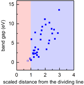
Figure 5: SISSO for classification. Correlation between the band gap of the non-metals and the scaled coordinate from the dividing line.

Beyond the training: Significance of the “distance” from the dividing line. Figure 5 depicts the experimental band gap of the insulators vs. the scaled distance from the dividing line, i.e., the dimensionless ratio between the $x$-projection of its descriptor versus the $x$-projection of the dividing line corresponding to the $y$-projection of its descriptor value. With this rescaling, the dividing line corresponds to the vertical line $x=1$ The trend of the data points reveals that the descriptor found by SISSO — trained only on a categorical property — includes a quantitative, albeit approximate, account of how strongly an insulator is far from being a metal, by locating materials with large band gaps further from the line than small-gap materials.

General remarks on the descriptor$\rightarrow$property relationship identified by SISSO. As clear from the two application cases presented here, the equations found by SISSO are not necessarily unique and all components of the descriptors may change at each added dimension. This reflects the approximate nature of the equations and the unavoidable relationships among features (one or more primary features may be accurately described by nonlinear functions of a subset of the remaining features). We also note that the mathematical constraints imposed in order to obtain solutions efficiently (linear combination of nonlinear functions for the continuous-property case and minimally overlapping convex hulls in the classification case), are very flexible but not complete. I.e., the found descriptor$\rightarrow$property relationship is intrinsically approximate.

Conclusions

We have presented an efficient approach for extracting effective materials descriptors out of huge and possibly strongly correlated features spaces. This algorithm, called SISSO (sure independence screening and sparsifying operators) tackles huge spaces while retaining the effectiveness of compressed sensing. Specifically, SISSO is built to work also (but not limited to) when only relatively small training sets are available. SISSO autonomously finds the best descriptor from a combination of features (physical properties), and it is capable of determining the ones not relevant to the problem, so that the features space can be further optimized. SISSO identifies the descriptor $\rightarrow$ property relationship in terms of an analytical equation. It does not need to be exact — a simple, analytical descriptor $\rightarrow$ property function may not even exist — but it is the most accurate expression given the available features space. If an exact, analytic expression does indeed exist, SISSO is expected to find it if included in the features space.

SISSO shows superior advantages with respect to other established methods, e.g., OMP and LASSO as well as the software Eureqa, especially when dealing with a correlated features spaces. SISSO does not have the limitation of LASSO, which suffers with large and highly correlated features spaces. Currently, the only issue of SISSO is the required computer memory needed to handle the features space, and efforts are underway for more efficient implementations. Our approach is benchmarked on the quantitative modeling of enthalpy differences for a set of zinc-blende and rock-salt prototypes and applied to the metal/insulator classification of binaries. The robustness of the classification is corroborated by the proper reproduced insulator$\leftrightarrow$metal transitions, which allows to predict a set of systems for further experimental analyses.

Appendix

In this appendix, we present details on the metal/insulator-classification application.
Primary features. Descriptors are to be identified by SISSO from a systematically-constructed large/huge features space in which components are generated by recursively transforming a set of input primary features, $\Phi_{0}$, via algebraic operations, $\bm{\hat{H}}\equiv\{I,+,-,\times,/,{\rm exp},{\rm log},|-|,\sqrt{\ },^{-1},^{2},^{3}\}$. Primary features usually comprise of properties of isolated atoms (atomic features) and properties of the materials (composition and geometry). For the test on binaries’ metal/nonmetal classification, the following is the full list of considered primary features:. (1) first ionization energy, $I\!E_{A}$ ($A$-species) and $I\!E_{B}$ ($B$-species); (2) electron affinity, $E\!A_{A}$ and $E\!A_{B}$; (3) atom covalent radius, $r_{\rm covA}$ and $r_{\rm covB}$; (4) Pauling electronegativity, $\chi_{A}$ and $\chi_{B}$; (5) valence, $v_{A}$ (#valence electrons) and $v_{B}$ ($8-$#valence electrons); (6) coordination number, $C\!N_{A}$ (#nearest neighbor $B$ of $A$) and $C\!N_{B}$; (7) interatomic distance between $A$ and $B$ in crystal, $d_{AB}$; (8) atomic composition $x_{A}$ (or $x_{B}=1-x_{A}$; and (9) the ratio of the cell volume to the total atom volume in the unit cell of the crystal, $V_{\rm cell}/\sum{V_{\rm atom}}$ ($V_{\rm atom}=4{\pi}r_{\rm cov}^{3}/3$).

Table 1: Dependence of the metal-insulator classification descriptors on the prototypes of training binary materials.

prototypes	#materials	primary features	descriptor	class.
NaCl	132	$I\!E_{A}$, $I\!E_{B}$, $\chi_{A}$, $\chi_{B}$, $r_{\rm covA}$, $r_{\rm covB}$, $E\!A_{A}$, $E\!A_{B}$, $v_{A}$, $v_{B}$, $d_{AB}$	$d_{1}:=\frac{I\!E_{A}I\!E_{B}(d_{AB}-r_{\rm covA})}{exp(\chi_{A})\sqrt{r_{\rm covB}}}$	100%
NaCl, CsCl, ZnS, CaF2, Cr3Si	217	$I\!E_{A}$, $I\!E_{B}$, $\chi_{A}$, $\chi_{B}$, $r_{\rm covA}$, $r_{\rm covB}$, $d_{AB}$, $C\!N_{A}$, $C\!N_{B}$	$d_{1}:=\frac{I\!E_{B}d_{AB}^{2}}{\chi_{A}r_{\rm covA}^{2}\sqrt{C\!N_{B}}}$, $d_{2}:=\frac{I\!E_{A}^{2}r_{\rm covB}\log{(I\!E_{A})}|r_{\rm covA}-r_{\rm covB}|}{C\!N_{B}}$	100%
NaCl, CsCl, ZnS, CaF2, Cr3Si, SiC, TiO2, ZnO, FeAs, NiAs	260	$I\!E_{A}$, $I\!E_{B}$, $\chi_{A}$, $\chi_{B}$, $r_{\rm covA}$, $r_{\rm covB}$, $d_{AB}$, $C\!N_{A}$, $C\!N_{B}$	$d_{1}:=\frac{d_{AB}/r_{\rm covA}-\chi_{A}/\chi_{B}}{\exp{(C\!N_{B}/I\!E_{B})}}$, $d_{2}:=\frac{r_{\rm covA}^{3}d_{AB}I\!E_{B}}{\left|\chi_{B}/\chi_{A}-|C\!N_{B}-C\!N_{A}|\right|}$	99.6%
NaCl, CsCl, ZnS, CaF2, Cr3Si, SiC, TiO2, ZnO, FeAs, NiAs	260	$I\!E_{A}$, $I\!E_{B}$, $\chi_{A}$, $\chi_{B}$, $x_{A}$, $x_{B}$, $V_{\rm cell}/\sum{V_{\rm atom}}$	$d_{1}:=\frac{V_{\rm cell}}{\sum{V_{\rm atom}}}\frac{\sqrt{\chi_{B}}}{\chi_{A}}$, $d_{2}:=\frac{I\!E_{A}I\!E_{B}}{\exp{(V_{\rm cell}/\sum{V_{\rm atom}})}}$	99.6%1
NaCl, CsCl, ZnS, CaF2, Cr3Si, SiC, TiO2, ZnO, FeAs, NiAs, Al2O3, La2O3, Th3P4, ReO3, ThH2	299	$I\!E_{A}$, $I\!E_{B}$, $\chi_{A}$, $\chi_{B}$, $x_{A}$, $x_{B}$, $V_{\rm cell}/\sum{V_{\rm atom}}$	$d_{1}:=\frac{x_{B}}{\sum{V_{\rm atom}}/V_{\rm cell}}\frac{I\!E_{B}\sqrt{\chi_{B}}}{\chi_{A}}$, $d_{2}:=\chi_{A}^{2}\left||1-2x_{A}|-x_{A}^{2}\frac{\chi_{B}}{\chi_{A}}\right|$	99.0%

It is critical to limit the redundant and unnecessary primary features in $\Phi_{0}$ to enhance computational performance (the size of features space $\Phi_{n}$ increases very fast with $\#\Phi_{0}$) and to increase SIS success rate: the higher #subspace/$\#\Phi$ the higher the probability that SIS subspaces contain the best models. Starting from an empty $\Phi_{0}$, few primary features are added. SISSO is then applied to identify the best model, with $\bm{\hat{H}}$ as operators space. If an appropriate quality of the model is not achieved (e.g., the number of correctly classified materials is lower than a desired threshold)), other primary features are added in $\Phi_{0}$ to check for improvements. Primary features preserved in $\Phi_{0}$ may become redundant or unnecessary on a later stage, e.g. when new ones are added. To retain computationally manageable sizes of the features space, tests are performed to remove those primary features that either are never appearing in the identified descriptor or that do not improve the performance of the model (in this specific case, when the number of correctly classified materials does not increase). Eventually, $\Phi_{0}$ will converge to the best possible small set of primary features, along with the best models that can be generated from it.

Data variety. The influence of data variety on the descriptors is investigated and Table 1 shows how the metal-insulator classification descriptors depend on the prototypes of training materials.

The first calculation starts with a data set of all the available materials (132) in NaCl-prototype. The initial features space, $\Phi_{0}$, contains the primary features of all the 10 atomic parameters (Table 1), and one structural parameter of interatomic distance $d_{AB}$ to capture the geometrical differences between the training rock-salt materials. SISSO is then applied: (1) $\Phi_{3}$ is constructed; (2) the best descriptor is identified from $\Phi_{3}$ for classifying the metals and insulators with 100% accuracy. The simple descriptor is shown in Table 1. It indicates that a rock-salt compound tends to become non metal when the large interatomic distance is decreased with the radius of species $A$.

Next, the number of prototypes is increased to 5, for a total of 217 materials. However, with the previous $\Phi_{0}$ and calculation-settings, SISSO fails to identify a descriptor having perfect classification (there are 7 points in the overlap-region between the metal and non metal domains). The non-optimal outcome indicates that the classification depends on primary features not yet considered. First, $\Phi_{0}$ is slimmed by reducing its size to 7 — $E\!A_{A}$, $E\!A_{B}$, $v_{A}$, and $v_{B}$ are removed — without affecting the quality of the predictions (8 points in the overlap-region). Second, two new features $C\!N_{A}$ and $C\!N_{B}$ are added ($\#\Phi_{0}\rightarrow 9$) to describe the different coordination environments of the prototypes. SISSO finds a 2D descriptor from the constructed $\Phi_{3}$ with 100% classification, shown in Table 1. From the descriptor, the geometrical differences between training materials are captured by the two features of $d_{AB}$ and $C\!N_{B}$: systems belonging to such 5 prototypes with large $d_{AB}$ and small $C\!N_{B}$ tend to be non metals.

The number of prototypes is increased to 10, for a total of 260 materials. As shown in Table 1, with the previous $\#\Phi_{0}=9$, the identified best descriptors is 2D have 99.6% classification (only one point, YP-compound in NaCl-prototype, is misclassified). Although the classification is excellent, the descriptor is complicate. Searching for a simplification, new primary features of atomic composition $x_{A}$, $x_{B}$, and $V_{\rm cell}/\sum{V_{\rm atom}}$ are introduced to replace $r_{\rm covA}$, $r_{\rm covB}$, $d_{AB}$, $C\!N_{A}$, and $C\!N_{B}$, leading to $\#\Phi_{0}\rightarrow 7$. With the same training materials, SISSO finds a much simple descriptor having the same accuracy of 99.6% (YP-compound remains misclassified). This result shows that the choice of proper primary features leads to descriptors’ simplification.

Finally, all the available 15 prototypes of binary materials (299) are considered and used with the 7 primary features in $\Phi_{0}$. With a constructed $\Phi_{3}$ of size $10^{8}$, SISSO identifies the best 2D descriptor with a classification accuracy of 99.0% (three misclassified compounds: YP-compound in NaCl-prototype, Th₃As₄ and La₃Te₄ in Th₃P₄-prototype). When new information — compounds and/or prototypes — is added, the functional form of the descriptors adapts. For predictive models, the data set requires all necessary information, e.g., by uniform sampling of the whole chemical and configurational space of the property of interest. The above 15 prototypes are not all the available prototypes for binary materials, and the layered materials (e.g., MoS₂, and those materials having $A-A$ or $B-B$ dimers, e.g., FeS₂, are not included) as the presented model is strictly illustrative of the method.

Reproducibility. To enable reproducibility, online tutorials where results can be interactively reproduced (and extended) are presented within the framework of the NOMAD Analytics-Toolkit (analytics-toolkit.nomad-coe.eu).
For the RS/ZB benchmark application:
analytics-toolkit.nomad-coe.eu/tutorial-SIS.
For the metal-nonmetal classification:
analytics-toolkit.nomad-coe.eu/tutorial-metal-nonmetal. The SISSO code, as used for the work presented here, but ready for broader applications is open source and can be found at github.com/rouyang2017/SISSO.

References

- (1) Office of Science and Technology Policy, White House, Materials Genome Initiative for Global Competitiveness, https://obamawhitehouse.archives.gov/mgi (2011).
- (2) S. Curtarolo, G. L. W. Hart, W. Setyawan, M. J. Mehl, M. Jahnátek, R. V. Chepulskii, O. Levy, and D. Morgan, “AFLOW: software for high-throughput calculation of material properties”, http://materials.duke.edu/aflow.html (2010).
- (3) A. Jain, G. Hautier, C. J. Moore, S. P. Ong, C. C. Fischer, T. Mueller, K. A. Persson, and G. Ceder, A high-throughput infrastructure for density functional theory calculations, Comput. Mater. Sci. 50, 2295–2310 (2011).
- (4) J. E. Saal, S. Kirklin, M. Aykol, B. Meredig, and C. Wolverton, Materials Design and Discovery with High-Throughput Density Functional Theory: The Open Quantum Materials Database (OQMD), JOM 65, 1501–1509 (2013).
- (5) D. D. Landis, J. Hummelshøj, S. Nestorov, J. Greeley, M. Dułak, T. Bligaard, J. K. Nørskov, and K. W. Jacobsen, The Computational Materials Repository, Comput. Sci. Eng. 14, 51–57 (2012).
- (6) A. A. White, Big data are shaping the future of materials science, MRS Bull. 38, 594–595 (2013).
- (7) L. M. Ghiringhelli, J. Vybiral, S. V. Levchenko, C. Draxl, and M. Scheffler, Big data of materials science: Critical role of the descriptor, Phys. Rev. Lett. 114, 105503 (2015).
- (8) S. R. Kalidindi and M. De Graef, Materials data science: current status and future outlook, Annu. Rev. Mater. Res. 45, 171–193 (2015).
- (9) W. Sun, S. T. Dacek, S. P. Ong, G. Hautier, A. Jain, W. D. Richards, A. C. Gamst, K. A. Persson, and C. Gerbrand, The thermodynamic scale of inorganic crystalline metastability, Science Advances 2, e1600225 (2016).
- (10) E. Perim, D. Lee, Y. Liu, C. Toher, P. Gong, Y. Li, W. N. Simmons, O. Levy, J. J. Vlassak, J. Schroers, and S. Curtarolo, Spectral descriptors for bulk metallic glasses based on the thermodynamics of competing crystalline phases, Nat. Commun. 7, 12315 (2016).
- (11) L. Ward, A. Agrawal, A. Choudhary, and C. Wolverton, A general-purpose machine learning framework for predicting properties of inorganic materials, NPJ Comput. Mater. 2, 16028 (2016).
- (12) O. Isayev, C. Oses, C. Toher, E. Gossett, S. Curtarolo, and A. Tropsha, Universal fragment descriptors for predicting electronic properties of inorganic crystals, Nat. Commun. 8, 15679 (2017).
- (13) K. Fujimura, A. Seko, Y. Koyama, A. Kuwabara, I. Kishida, K. Shitara, C. Fisher, H. Moriwake, and I. Tanaka, Accelerated Materials Design of Lithium Superionic Conductors Based on First‐Principles Calculations and Machine Learning Algorithms, Adv. Energy Mater. 3, 980–985 (2013).
- (14) S. Curtarolo, G. L. W. Hart, M. Buongiorno Nardelli, N. Mingo, S. Sanvito, and O. Levy, The high-throughput highway to computational materials design, Nat. Mater. 12, 191–201 (2013).
- (15) B. Meredig and C. Wolverton, A hybrid computational-experimental approach for automated crystal structure solution, Nat. Mater. 12, 123–127 (2013).
- (16) C. C. Fischer, K. J. Tibbetts, D. Morgan, and G. Ceder, Predicting crystal structure by merging data mining with quantum mechanics, Nat. Mater. 5, 641–646 (2006).
-
(17)
NOMAD: Novel Materials Discovery
https://www.nomad-coe.eu (2015). - (18) C. Draxl and M. Scheffler, NOMAD: The FAIR Concept for Big-Data-Driven Materials Science, MRS Bull., in press (2018); arXiv:cond-mat/1805.05039 .
- (19) A. Bartók, P. Albert, M. C. Payne, R. Kondor, and G. Csányi, Gaussian approximation potentials: The accuracy of quantum mechanics, without the electrons, Phys. Rev. Lett. 104, 136403 (2010).
- (20) J. Carrete, N. Mingo, S. Wang, and S. Curtarolo, Nanograined Half-Heusler Semiconductors as Advanced Thermoelectrics: An Ab Initio High-Throughput Statistical Study, Adv. Func. Mater. 24, 7427–7432 (2014).
- (21) K. Rajan, Materials informatics: The materials “gene” and big data, Annu. Rev. Mater. Res. 45, 153–169 (2015).
- (22) T. Mueller, A. G. Kusne, and R. Ramprasad, Machine Learning in Materials Science (John Wiley & Sons, Inc, 2016), pp. 186–273.
- (23) C. Kim, G. Pilania, and R. Ramprasad, From organized high-throughput data to phenomenological theory using machine learning: the example of dielectric breakdown, Chem. Mater. 28, 1304–1311 (2016).
- (24) F. A. Faber, A. Lindmaa, O. A. von Lilienfeld, and R. Armiento, Machine Learning Energies of 2 Million Elpasolite Crystals, Phys. Rev. Lett. 117, 135502 (2016).
- (25) K. Takahashi and Y. Tanaka, Materials informatics: a journey towards material design and synthesis, Dalton Trans. 45, 10497–10499 (2016).
- (26) A. Bartók, S. De, C. Poelking, N. Bernstein, J. Kermode, G. Csányi, and M. Ceriotti, Machine learning unifies the modeling of materials and molecules, Sci. Adv. 3, 1701816 (2017).
- (27) B. R. Goldsmith, M. Boley, J. Vreeken, M. Scheffler, and L. M. Ghiringhelli, Uncovering structure-property relationships of materials by subgroup discovery, New J. Phys. 19, 013031 (2017).
- (28) T. L. Pham, N. D. Nguyen, V. D. Nguyen, H. Kino, T. Miyake, and H. C. Dam, Learning structure-property relationship in crystalline materials: A study of lanthanide–transition metal alloys, J. Chem. Phys. 148, 204106 (2018).
- (29) T. Hey, S. Tansley, and K. Tolle, The Fourth Paradigm: Data-Intensive Scientific Discovery (Microsoft Research, 2009).
- (30) A. Agrawal and A. Choudhary, Perspective: Materials informatics and big data: Realization of the “fourth paradigm” of science in materials science, APL Mater. 4, 053208 (2016).
- (31) L. M. Ghiringhelli, J. Vybiral, E. Ahmetcik, R. Ouyang, S. V. Levchenko, C. Draxl, and M. Scheffler, Learning physical descriptors for materials science by compressed sensing, New J. Phys. 19, 023017 (2017).
- (32) E. J. Candès and M. B. Wakin, An introduction to compressive sampling, IEEE Signal Proc. Mag. 25, 21–30 (2008).
- (33) L. J. Nelson, G. L. Hart, F. Zhou, V. Ozoliņš, et al., Compressive sensing as a paradigm for building physics models, Phys. Rev. B 87, 035125 (2013).
- (34) E. J. Candès, J. Romberg, and T. Tao, Robust uncertainty principles: Exact signal reconstruction from highly incomplete frequency information, IEEE Trans. Inf. Theory 52, 489–509 (2006).
- (35) D. L. Donoho, Compressed sensing, IEEE Trans. Inform. Theory 52, 1289–1306 (2006).
- (36) R. Tibshirani, Regression shrinkage and selection via the lasso, J. R. Statist. Soc. B 58, 267–288 (1996).
- (37) P. Sondhi, Feature construction methods: a survey, Tech. rep., sifaka.cs.uiuc.edu (2009).
- (38) I. Guyon and A. Elisseeff, An introduction to variable and feature selection, J. Mach. Learn. Res. 3, 1157–1182 (2003).
- (39) P. Breen, Algorithms for sparse approximation, Tech. rep., School Math., Univ. Edinburgh, Edinburgh, U.K., 4 Year Project Report (2009).
- (40) M. Schmidt and H. Lipson, Distilling free-form natural laws from experimental data, Science 324, 81–85 (2009).
- (41) The -norm of a vector is the number of its non-zero components.
- (42) D. L. Donoho and M. Elad, Optimally sparse representation in general (nonorthogonal) dictionaries via minimization, Proc. Natl. Acad. Sci. U.S.A. 100, 2197–2202 (2003).
- (43) The -norm is the sum of the absolute values of the components of a vector.
- (44) S. G. Mallat and Z. Zhang, Matching pursuits with time-frequency dictionaries, IEEE Trans. Signal Process 41, 3397–3415 (1993).
- (45) Y. C. Pati, R. Rezaiifar, and P. S. Krishnaprasad, Orthogonal matching pursuit: Recursive function approximation with applications to wavelet decomposition, in The Twenty-Seventh Asilomar Conf.: Signals, Systems and Computers (IEEE, Pacific Grove, CA, Nov. 1993), vol. 1, pp. 40–44.
- (46) J. A. Tropp and A. C. Gilbert, Signal recovery from random measurements via orthogonal matching pursuit, IEEE Trans. Inform. Theory 53, 4655–4666 (2007).
- (47) J. A. Tropp, Greed is good: Algorithmic results for sparse approximation, IEEE Trans. Inform. Theory 50, 2231–2242 (2004).
- (48) E. J. Candès, Y. C. Eldar, D. Needell, and P. Randall, Compressed sensing with coherent and redundant dictionaries, Appl. Comput. Harmon. Anal. 31, 59–73 (2011).
- (49) J. Fan and J. Lv, Sure independence screening for ultrahigh dimensional feature space, J. R. Statist. Soc. B 70, 849–911 (2008).
- (50) J. Fan, R. Samworth, and Y. Wu, Ultrahigh dimensional feature selection: beyond the linear model, J. Mach. Learn. Res. 10, 2013–2038 (2009).
- (51) E. J. Candès and J. Romberg, Sparsity and incoherence in compressive sampling, Inverse Prob. 23, 969–985 (2007).
- (52) T. Hastie, R. Tibshirani, and J. Friedman, The elements of statistical learning, vol. 1 (Springer Series in Statistics, 2009), 2 edn.
- (53) J. Pearl, Causality: Models, Reasoning and Inference (Cambridge University Press, New York, NY, USA, 2009), 2nd edn.
- (54) P. Boufounos, M. F. Duarte, and R. G. Baraniuk, Sparse Signal Reconstruction from Noisy Compressive Measurements using Cross Validation, in 2007 IEEE/SP 14th Workshop on Statistical Signal Processing (2007), pp. 299–303.
- (55) R. Ward, Compressed Sensing With Cross Validation, IEEE Trans. Inf. Theory 55, 5773–5782 (2009).
- (56) A. F. Bialon, T. Hammerschmidt, and R. Drautz, Three-parameter crystal-structure prediction for sp-d-valent compounds, Chem. Mater. 28, 2550–2556 (2016).
- (57) https://www.webelements.com
- (58) https://materials.springer.com
- (59) R. Ouyang, S. Curtarolo, E. Ahmetcik, M. Scheffler, and L. M. Ghiringhelli, On the identification of predictive physical models for material properties, to be published (2018).
- (60) T. Joachims, Making large-scale SVM learning practical, Tech. rep., Technical Report, SFB 475: Komplexitätsreduktion in Multivariaten Datenstrukturen, Universität Dortmund (1998).
- (61) M. F. Ashby, A first report on deformation-mechanism maps, Acta Mater. 20, 887–897 (1972).
- (62) D. G. Pettifor, A chemical scale for crystal-structure maps, Solid State Commun. 51, 31–34 (1984).
- (63) D. G. Pettifor, The structures of binary compounds. I. Phenomenological structure maps, J. Phys. C: Solid State Phys. 19, 285–313 (1986).
- (64) O. Isayev, D. Fourches, E. N. Muratov, C. Oses, K. Rasch, A. Tropsha, and S. Curtarolo, Materials Cartography: Representing and Mining Materials Space Using Structural and Electronic Fingerprints, Chem. Mater. 27, 735–743 (2015).
- (65) B. Cordero, V. Gómez, A. E. Platero-Prats, M. Revés, J. Echeverría, E. Cremades, F. Barragán, and S. Alvarez, Covalent radii revisited, Dalton Trans. pp. 2832–2838 (2008).
- (66) M. Pardo and J. Flahaut, Les systémes CaTe-LaTe3 formés avec les éléments des terres rares et l’yttrium, Bulletin de la Societe Chimique de France pp. 6–9 (1969).
- (67) P. J. Markowski, Z. Henkie, and A. Wojakowski, Electronic properties of Th3As4-U3As4 solid solutions, Solid State Communications 32, 1119–1123 (1979).
- (68) C. Toher, C. Oses, J. J. Plata, D. Hicks, F. Rose, O. Levy, M. de Jong, M. D. Asta, M. Fornari, M. Buongiorno Nardelli, and S. Curtarolo, Combining the AFLOW GIBBS and Elastic Libraries to efficiently and robustly screen thermomechanical properties of solids, Phys. Rev. Mater. 1, 015401 (2017).