Security considerations for Galois non-dual RLWE families

Abstract

We explore further the hardness of the non-dual discrete variant of the Ring-LWE problem for various number rings, give improved attacks for certain rings satisfying some additional assumptions, construct a new family of vulnerable Galois number fields, and apply some number theoretic results on Gauss sums to deduce the likely failure of these attacks for 2-power cyclotomic rings and unramified moduli.

1 Introduction

Lattice-based cryptography was introduced in the mid 1990s in two different forms, independently by Ajtai-Dwork [1] and Hoffstein-Pipher-Silverman [12]. Thanks to the work of Stehlé-Steinfeld [19], we now understand the NTRU cryptosystem introduced by Hoffstein-Pipher-Silverman to be a variant of a cryptosystem which has security reductions to the Ring Learning With Errors (RLWE) problem. The RLWE problem was introduced in [14] as a version of the LWE problem [17]: both problems have reductions to hard lattice problems and thus are interesting for practical applications in cryptography. RLWE depends on a number ring $R$, a modulus $q$, and an error distribution. As such, it has added structure (the ring), which allows for greater efficiency, but also in some cases additional attacks.

The hardness of RLWE is crucial to cryptography, in particular as the basis of numerous homomorphic encryption schemes [2, 3, 4, 5, 6, 13, 19]. One main theoretical result in this direction is the security reduction theorem in [14], which reduces certain GapSVP problems in ideal lattices over $R$ to RLWE, when the RLWE error distribution is sufficiently large and of a prescribed form. Although so far in practical cryptographic applications only cyclotomic rings are used, it is important to study the hardness of RLWE for general number rings, moduli and error distributions, so as to understand the boundaries of security in the parameter space. Recently, new attacks on the so-called non-dual discrete variant of the RLWE problem for certain number rings, error distributions, and special moduli were introduced [7, 8, 9, 10, 11]. The RLWE problem reduces to its discrete variant; and the non-dual RLWE problem is equivalent to the dual problem up to a change in the error distribution, so that non-dual RLWE may be viewed simply as a certain choice of error distribution in the parameter space of RLWE. The term RLWE is sometimes reserved for spherical Gaussian distributions.

This paper is an extension of [9], and here we explore further the hardness of the non-dual discrete variant of the RLWE problem for various number rings. We:

1. construct a new family of vulnerable Galois number fields,

2. improve the runtime of the attacks for certain rings satisfying some additional assumptions, and

3. apply some number theoretic results on Gauss sums to deduce the likely failure of these attacks for 2-power cyclotomic rings.

In cryptographic applications, it is most efficient to sample the error distribution coordinate-wise according to a polynomial basis for the ring. For $2$-power cyclotomic rings, which are monogenic with a well-behaved power basis, it is justified to sample the RLWE error distribution directly in the polynomial basis for the ring, according to results in [5, 10, 14], where this error distribution choice is called Polynomial Learning With Errors (PLWE). Precisely, the PLWE (polynomial error), RLWE (meaning a spherical Gaussian), and non-dual RLWE problems are equivalent up to a scaling and rotation of the error distribution for $2$-power cyclotomic fields. However, in general number rings the error distribution may be distorted by a general linear transformation when moving from one problem to another [11]. For certain choices of ring and modulus, efficient attacks on PLWE were presented in [10]. In [11], these attacks were extended to apply to the decision version of the non-dual RLWE problem in certain rings, and in [8, 9], attacks on the search version of the RLWE problem for certain choices of ring and modulus were presented.

1.1 Summary of contributions

• In Section 3, we present an improvement to the attack in [9, Section 4] and use it to dramatically cut down the runtime of the attacks on the weak instances found in [9, Section 5].

• In Section 4, we present a new infinite family of Galois number fields vulnerable to our attack in [9, Section 4], where the relative standard deviation parameter is allowed to grow to infinity, and we give a table of examples.

• In Section 5, we analyze the security of 2-power cyclotomic fields with unramified moduli under our attack. We prove Theorem 5.2, which gives an upper bound on the statistical distance between an approximated non-dual RLWE error distribution, reduced modulo a prime ideal $\mathfrak{q}$, and the uniform distribution on $R/\mathfrak{q}$. We conclude that the 2-power cyclotomic rings are safe against our attack when the modulus $q$ is unramified with small residue degree (1 or 2), and is not too large ($q<m^{2}$).

Acknowledgements We thank Chris Peikert, Igor Shparlinski, Léo Ducas and Ronald Cramer for helpful discussions.

2 Background

2.1 Discrete Gaussian on lattices

Recall that a lattice in $\mathbb{R}^{n}$ is a discrete subgroup of $\mathbb{R}^{n}$ of rank $n$. For $r>0$, let $\rho_{r}(x)=e^{-||x||^{2}/r^{2}}$.

Definition 1

For a lattice $\Lambda\subset\mathbb{R}^{n}$ and $r>0$, the discrete Gaussian distribution on $\Lambda$ with width $r$ is:

$$D_{\Lambda,r}(x)=\frac{\rho_{r}(x)}{\sum_{y\in\Lambda}\rho_{r}(y)},\,\forall x\in\Lambda.$$

2.2 Non-dual RLWE

A non-dual discrete RLWE instance is specified by a ring $R$, a positive integer $q$ and an error distribution $\chi$ over $R$. Here $R$ is normally taken to be the ring of integers of some number field $K$ of degree $n$. The integer $q$, called the modulus, is often taken to be a prime number. We then fix an element $s\in R/qR$ called the secret.

Let $\iota:K\to\mathbb{R}^{n}$ be the adjusted canonical embedding defined as follows. Suppose $\sigma_{1},\ldots,\sigma_{r_{1}},\sigma_{r_{1}+1},\ldots,\sigma_{n}$ are the distinct embeddings of $K$, such that $\sigma_{1},\cdots,\sigma_{r_{1}}$ are the real embeddings and $\sigma_{r_{1}+r_{2}+j}=\overline{\sigma_{r_{1}+j}}$ for $1\leq j\leq r_{2}$. We define $\iota:K\to\mathbb{R}^{n}$ by

$$x\mapsto(\sigma_{1}(x),\cdots,\sigma_{r_{1}}(x),\sqrt{2}\real(\sigma_{r_{1}+1}(x)),\sqrt{2}\imaginary(\sigma_{r_{1}+1}(x)),\cdots,$$

$$\sqrt{2}\real(\sigma_{r_{1}+r_{2}}(x)),\sqrt{2}\imaginary(\sigma_{r_{1}+r_{2}}(x))).$$

Then the non-dual discrete RLWE error distribution is the discrete Gaussian distribution $D_{\iota(R),r}$.

Definition 2

Fix $R,q,r$ as above. Let $R_{q}$ denote the quotient ring $R/qR$. Then a non-dual RLWE sample is a pair

$$(a,b=as+e)\in R_{q}\times R_{q},$$

where the first coordinate $a$ is chosen uniformly at random in $R_{q}$, and $e$ is a sampled from the discrete Gaussian $D_{\iota(R),r}$, considered modulo $q$.

Definition 3 (Non-dual Search RLWE)

Given arbitrarily many non-dual RLWE samples, determine the secret $s$.

Definition 4 (Non-dual Decision RLWE)

Given arbitrarily many samples in $R_{q}\times R_{q}$, which are either non-dual RLWE samples for a fixed secret $s$, or uniformly random samples, determine which.

2.3 Comparing RLWE with non-dual RLWE

In the original work [14], the RLWE problem is introduced using the dual ring $R^{\vee}$. Specifically, for the discrete variant, $s\in R_{q}^{\vee}:=R^{\vee}/qR^{\vee}$, and an RLWE sample is taken to be of the form

$$(a,b=as+e)\in R_{q}\times R_{q}^{\vee},$$

where $e$ is sampled from $D_{\iota(R^{\vee}),r}$, then considered modulo $q$.

If the dual ring $R^{\vee}$ is principal as a fractional ideal, i.e., $R^{\vee}=tR$, then each non-dual instance is equivalent to a dual instance, by mapping a sample $(a,b)$ to $(a,tb)$, and vice versa. If $R^{\vee}$ is not principal, there are still inclusions $R^{\vee}\subset t_{1}R$ and $R\subset t_{2}R^{\vee}$, so that one can reduce dual and non-dual versions of the problem to one another. In either case, the reduction comes at the cost of distorting the error distribution.

For the infinite family constructed in Section 4, the dual ring $R^{\vee}$ is indeed principal (see Lemma 3 in Section 4). Note that multiplying by this field element $t$ changes a spherical Gaussian to an elliptical Gaussian, so the two equivalent instances will have different error shapes.

Elliptical Gaussians are the most important class of error distributions for general rings, since in [14, Theorem 4.1], the reduction from hard lattice problems is to a class of RLWE problems where the distributions are elliptical Gaussians. Theorem 5.2 of [14] provides a further security reduction to decision RLWE with spherical Gaussian errors, but it is only stated for cyclotomic rings.

2.4 Comparing discrete and continuous errors

Restricting now to the non-dual setup, there are still two variants of RLWE based on the form of the spherical errors: the continuous variant samples errors from spherical Gaussian on the space $K_{\mathbb{R}}=\iota(K\otimes_{\mathbb{Q}}\mathbb{R})$ (here we extend $\iota$ linearly), so that samples have the form

$$(a,b=as+e)\in R_{q}\times K_{\mathbb{R}}/qR,$$

whereas the discrete variant samples from a discrete Gaussian $D_{\iota{R},r}$ on the lattice $R$, as defined above.

There is no known equivalence between the discrete problem and its continuous counterpart in general. However, the continuous problem reduces to the discrete one. Specifically, given a continuous sample $(a,b)\in R_{q}\times K_{\mathbb{R}}/qR$, one can perform a rounding on the second coordinate to get a discrete sample $(a,[b])\in R_{q}\times R_{q}$. However, there is no obvious map in the reverse direction.

2.5 Search and decision RLWE problems

Let $\mathfrak{q}$ be a prime ideal of $K$ lying above $q$; then the RLWE problem modulo $\mathfrak{q}$ means discovering $s\mod{\mathfrak{q}}$ from arbitrarily many RLWE samples. In [14] the authors gave a polynomial time reduction from search to decision for cyclotomic number fields and totally split primes, using the RLWE modulo $\mathfrak{q}$ as an intermediate problem. Their proof can be applied to prove a similar search-to-decision reduction for non-dual RLWE, when the underlying number field is Galois and the modulus $q$ is unramified [9, 10]. Moreover, the search-to-decision is most efficient when the residue degree of $q$ is small. What is important in our paper is that for the instances in Section 3 and 4, our attacks on RLWE modulo $\mathfrak{q}$ could be efficiently transferred to attack the search problem.

2.6 Comparing non-dual RLWE with PLWE for 2-power cyclotomic fields

For cryptographic applications, it is perhaps natural to consider the PLWE error distribution on $R$: assuming the ring $R$ is monogenic, i.e., $R=\mathbb{Z}[x]/(f(x))$, then a sample from the PLWE error distribution is $e=\sum_{i=0}^{n-1}e_{i}x^{i}$, where the $e_{i}$ are “small errors”, sampled independently from some error distribution over $\mathbb{Z}$ (e.g. a discrete Gaussian distribution).

In general number fields, a PLWE distribution differs greatly from the non-dual RLWE distribution (see [ELOS] for an effort to quantify the distance between the two distributions using spectral norms). However, for 2-power cyclotomic fields it turns out that the two error distributions are equivalent up to a factor of $\sqrt{n}$. Since this fact is used in Section 5, we give a proof below.

Lemma 1

Let $m=2^{d}$ be a power of 2 and let $R=\mathbb{Z}[\zeta_{m}]$. Consider the PLWE error distribution on $R$, i.e. samples $e=\sum_{i=0}^{n-1}e_{i}\zeta_{m}^{i}$, where $n=m/2$ and each $e_{i}$ follows the discrete Gaussian $D_{\mathbb{Z},r}$. Then this PLWE distribution is equal to the non-dual RLWE distribution $D_{\iota(R),r\sqrt{n}}$.

Proof

For an element $x=\sum_{i=0}^{n-1}x_{i}\zeta_{m}^{i}\in R$, the probability of $x$ being sampled by the PLWE distribution is proportional to $\prod_{i=0}^{n-1}\rho_{r}(x_{i})=\prod_{i=0}^{n-1}e^{-x_{i}^{2}/r^{2}}=e^{-||x||^{2}/r^{2}}$. On the other hand, one checks that $||\iota(x)||=\sqrt{n}||x||$. So the above probability is proportional to $e^{-||\iota(x)||^{2}/nr^{2}}$, which is the exactly the same for the distribution $D_{\iota(R),r\sqrt{n}}$. This completes the proof.

2.7 Scaling factors

As pointed out in [11], when analyzing the non-dual RLWE error distribution, one needs to take into account the sparsity of the lattice $\iota(R)$, measured by its covolume in $\mathbb{R}^{n}$. This covolume is equal to $|\operatorname{disc}(K)|^{1/2}$. In light of this, we define the scaled error width to be

$$r_{0}=\frac{r}{|\operatorname{disc}(K)|^{\frac{1}{2n}}}.$$

2.8 Overview of attack

We briefly review the method of attack in Section 4 of [9]. The basic principle of this family of attacks is to find a homomorphism

$$\rho:R_{q}\rightarrow F$$

to some small finite field $F$, such that the error distribution on $R_{q}$ is transported by $\rho$ to a non-uniform distribution on $F$. In this case, errors can be distinguished from elements uniformly drawn from $R_{q}$ by a statistical test in $F$, for example, by a $\chi^{2}$-test. The existence (or non-existence) of such a homomorphism depends on the parameters of the field, prime, and distribution in the setup of RLWE. In this section, we will describe parameters under which such a map exists.

Once such a map is known, the basic method of attack on Decision RLWE is as follows:

1. Apply $\rho$ to samples $(a,b)$ in $R_{q}\times R_{q}$, to obtain samples in $F\times F$.

2. Guess the image of the secret $\rho(s)$ in $F$, calling the guess $g$.

3. Compute the distribution of $\rho(b)-\rho(a)g$ for all the samples. If $g=\rho(s)$, this is the image of the distribution of the errors. Otherwise it is the image of a uniform distribution.

4. If the image looks uniform, try another guess $g$ until all are exhausted. If any non-uniform distribution is found, the samples are RLWE samples. Otherwise they are not.

Whenever $\mathfrak{q}$ is a prime ideal lying above $q$, then reduction modulo $\mathfrak{q}$ is a valid map

$$\rho:R_{q}\rightarrow R_{\mathfrak{q}}$$

for the attack above. This attack targets the RLWE modulo $\mathfrak{q}$ problem for some prime $\mathfrak{q}$ lying above $q$, and as noted above, it can be turned into an attack on the search variant of the problem, whenever $q$ is unramified and $K$ is Galois.

2.9 Comparison to related works

In an independent preprint ([7]) which appeared on eprint around the same time as our preprint, Castryck et al. also constructed an infinite family of vulnerable Galois number fields, where the error width can be taken to be $O(|\operatorname{disc}(K)|^{\frac{1}{n}-\epsilon})$ for any $\epsilon>0$. The asymptotic error width they obtained is wider than in our infinite family in Section 2. However, the method of attack is an errorless LWE linear algebra attack (based on short vectors), whereas our family is not susceptible to a linear algebra attack, and requires the novel techniques presented here and in [9].

3 An improved attack using cosets

In this section, we describe an improvement to our chi-square attack on RLWE mod $\mathfrak{q}$ outlined in Section 2.8 for a special case. As a result, we have an updated version of [9, Table 1], where we attacked each instance in the table in much shorter time. Note that the complexity of the previous attack in this special case is $O(nq^{3})$. In contrast, our new attack has complexity $O(nq^{2})$.

To clarify, the special case we consider in this section is characterised by the following assumptions (we need not be in the special family of the next section):

• The modulus $q$ is a prime of residue degree 2 in the number field $K$.

• There exists a prime ideal $\mathfrak{q}$ above $q$ such that the map $\rho:R_{q}\to R_{\mathfrak{q}}$ satisfies the following property: Let $e\in R_{q}$ be taken from the discrete RLWE error distribution. The probability that $\rho(e)$ lies in the prime subfield $\mathbb{F}_{q}$ of $\mathbb{F}_{q^{2}}$ is computationally distinguishable from $1/q$.

Granting these assumptions, we can distinguish the distribution of the “reduced error” $\rho(e)$ from the uniform distribution on $\mathbb{F}_{q^{2}}$. More precisely, the attack in [9] works exactly as we described in Section 4: with access to $\Omega(q)$ samples, one loops over all $q^{2}$ possible values of $\rho(s)$. It detects the correct guess $\rho(s)$ based on a chi-square test with two bins $\mathbb{F}_{q}$ and $\mathbb{F}_{q^{2}}\setminus\mathbb{F}_{q}$.

The distinguishing feature of the improved attack is to loop over the cosets of $\mathbb{F}_{q}$ of $\mathbb{F}_{q^{2}}$ instead of the whole space. Fix $t_{1},\cdots t_{q}$ to be a set of coset representatives for the additive group $\mathbb{F}_{q^{2}}/\mathbb{F}_{q}$. Recall that $s$ denotes the secret and $\rho:R_{q}\to R_{\mathfrak{q}}\cong\mathbb{F}_{q^{2}}$ is a reduction map modulo some fixed prime ideal $\mathfrak{q}$ lying above $q$. Then there exists a unique index $i$ such that $\rho(s)=s_{0}+t_{i}$ for some $s_{0}\in\mathbb{F}_{q}$. Our improved attack will recover $s_{0}$ and $t_{i}$ separately.

We start with an identity $b=as+e$, where $a,b,s,e\in\mathbb{F}_{q^{2}}$. We will regard $s$ as fixed and $a,b,e$ as random variables, such that $a$ is uniformly distributed in $\mathbb{F}_{q^{2}}\setminus\mathbb{F}_{q}$ and $b$ is uniformly distributed in $\mathbb{F}_{q^{2}}$. The reason why $a$ is not taken to be uniform will become clear later in this section. We use a bar to denote the Frobenius automorphism, i.e.,

$$\bar{a}\stackrel{{\scriptstyle def}}{{=}}a^{q},\,\forall a\in\mathbb{F}_{q^{2}}.$$

Then $\bar{b}=\bar{a}\bar{s}+\bar{e}$. Using the identity $s=s_{0}+t_{i}$ and subtracting, we obtain $\bar{b}-b-\overline{at_{i}}+at_{i}=s_{0}(\bar{a}-a)+\bar{e}-e$. Since $a\neq\bar{a}$, we can divide through by $\bar{a}-a$ and get

$$\frac{\bar{b}-b-\overline{at_{i}}+at_{i}}{\bar{a}-a}=s_{0}+\frac{\bar{e}-e}{\bar{a}-a}.$$

Now for each $1\leq j\leq q$, we can compute

$$m_{j}(a,b):=\frac{\bar{b}-b-\overline{at_{j}}+at_{j}}{\bar{a}-a}$$

with access to $a$ and $b$, but without knowledge of $s$ or $s_{0}$. Note that $m_{j}$ is in the prime field $\mathbb{F}_{q}$ by construction.

Proposition 1

For each $1\leq j\leq q$,
(1) If $j\neq i$, then $m_{j}(a,b)$ is uniformly distributed in $\mathbb{F}_{q}$, for RLWE samples $(a,b)$.
(2) If $j=i$, then $m_{j}(a,b)=s_{0}+\frac{\bar{e}-e}{\bar{a}-a}$.

We postpone the proof of Proposition 1 until the end of this section. Assuming the proposition, our improved attack works as follows: for $1\leq j\leq q$, we compute a set of $m_{j}$ from the samples. To avoid dividing by zero, we ignore the samples with $\rho(a)\in\mathbb{F}_{q}$ (which happens with probability $1/q$ since $\rho(a)$ is uniformly distributed). We then run a chi-square test on the $m_{j}$ values. If $j\neq i$, then the distribution should be uniform; if $j=i$, then $P(m_{i}=s_{0})=P(e\in\mathbb{F}_{q})$, which by our assumption is larger than $1/q$. Hence if we plot the histogram of the $m_{i}$ computed from the samples, we will see a spike at $s_{0}$. So we could recover $s_{0}$ as the element with the highest frequency, and output $\rho(s)=s_{0}+t_{i}$. We give the pseudocode of the attack below.

Algorithm 1 Improved chi-square attack on RLWE modulo $\mathfrak{q}$)

$K$ – a number field; $R$ – the ring of integers of $K$; $\mathfrak{q}$ – a prime ideal in $K$ above $q$ with residue degree 2; $\mathcal{S}$ – a collection of $M$ RLWE samples; $\beta>0$ – the parameter used for comparing $\chi^{2}$ values.

a guess of the value $s\pmod{\mathfrak{q}}$, or NOT-RLWE, or INSUFFICIENT-SAMPLES

Let $\mathcal{G}\leftarrow\emptyset$.

for $j$ in $1,\ldots,q$ do

     $\mathcal{E}_{j}\leftarrow\emptyset$.

     for $a,b$ in $\mathcal{S}$ do

         $\bar{a},\bar{b}\leftarrow a\pmod{\mathfrak{q}},b\pmod{\mathfrak{q}}$.

         $m_{j}\leftarrow\frac{\bar{b}-b-\overline{at_{j}}+at_{j}}{\bar{a}-a}.$

         add $m_{j}$ to $\mathcal{E}_{j}$.

     end for

     Run a chi-square test for uniform distribution on $\mathcal{E}_{j}$.

     if $\chi^{2}(\mathcal{E}_{j})>\beta$ then

         $s_{0}:=$ the element(s) in $\mathcal{E}_{j}$ with highest frequency.

         $s\leftarrow s_{0}+t_{j}$, add $s$ to $\mathcal{G}$.

     end if

end for

if $\mathcal{G}=\emptyset$ then return NOT-RLWE

else if $\mathcal{G}=\{s\}$ is a singleton then return $s$

elsereturn INSUFFICIENT-SAMPLES

end if

We analyze the complexity of our improved attack. There are $q$ iterations, each operating on $O(q)$ samples, and reduction of each sample is $O(n)$. So our new attack has complexity $O(nq^{2})$.

3.1 Examples of successful attacks

To illustrate the idea, we apply our improved attack to the instances in Table 1 of [9]. Comparing the last column with the current Table 1, we see that the runtime has been improved significantly.

Table 1: RLWE instances under our improved attack

$n$	$q$	$f$	$r_{0}$	no. samples	old runtime (in minutes)	new runtime (in minutes)
40	67	2	2.51	22445	209	3.5
60	197	2	2.76	3940	63	2.4
60	617	2	2.76	12340	8.2 $\times 10^{5}$ (est.)	21.3
80	67	2	2.51	3350	288.6	0.5
90	2003	2	3.13	60090	6.6 $\times 10^{4}$ (est.)	305
96	521	2	2.76	15630	4.5 $\times 10^{3}$ (est.)	21.7
100	683	2	2.76	20490	1.6 $\times 10^{4}$(est.)	36.5
144	953	2	2.51	38120	342.6	114.5

3.2 Proof of Proposition 1

For notational convenience, we let $A_{q}$ denote the set $\mathbb{F}_{q^{2}}\setminus\mathbb{F}_{q}$.

Lemma 2

Let the random variable $a$ be uniformly distributed in $A_{q}$. Suppose $e$ is a random variable with value in $\mathbb{F}_{q^{2}}$ independent of $a$. Fix $\delta\in A_{q}$ and $s_{0}\in\mathbb{F}_{q}$. Then

$$m_{\delta}=g_{\delta}+s_{0}+\frac{\bar{e}-e}{\bar{a}-a}$$

is uniformly distributed in $\mathbb{F}_{q}$. Here

$$g_{\delta}=\frac{\overline{a\delta}-a\delta}{\bar{a}-a}.$$

Proof

Since the uniform distribution is invariant under translation, we may assume $s_{0}=0$. We introduce a new set $V=\{x\in\mathbb{F}_{q^{2}}:\bar{x}=-x\}$. We claim that for any $c,d\in V$ with $c\neq 0$, we have $P(\bar{a}-a=c,\overline{a\delta}-a\delta=d)=\frac{1}{q(q-1)}$. To prove the claim, note that $V$ is an $\mathbb{F}_{q}$-vector space of dimension one, and we have the following $\mathbb{F}_{q}$-linear map $f_{\delta}:\mathbb{F}_{q^{2}}\to V^{2}$.

$$f_{\delta}:a\mapsto(\bar{a}-a,\overline{a\delta}-a\delta).$$

First we show $f_{\delta}$ is injective: if $f_{\delta}(a)=0$, then $a\in\mathbb{F}_{q}$ and thus $a(\bar{\delta}-\delta)=0$, so $a=0$. By dimension counting, $f_{\delta}$ is an isomorphism. Restricting to $A_{q}$, we see that $f_{\delta}|_{A_{q}}$ gives an isomorphism between $A_{q}$ and $(V\setminus\{0\})\times V$. This proves the claim.

Let $e^{\prime}=\frac{\bar{e}-e}{\bar{a}-a}$. For any $z\in\mathbb{F}_{q}$, we have

$$\quad P(g_{\delta}+e^{\prime}=z)$$

$$=\sum_{x+y=z}P(g_{\delta}=x,e^{\prime}=y)$$

$$=\sum_{x+y=z}\sum_{c\in V\setminus\{0\}}P(\bar{a\delta}-a\delta=xc,\bar{e}-e=yc,\bar{a}-a=c)$$

$$=\sum_{x+y=z,c\in V\setminus\{0\}}P(\bar{a\delta}-a\delta=xc,\bar{a}-a=c)P(\bar{e}-e=yc)$$

$$=\frac{1}{q(q-1)}\sum_{y\in\mathbb{F}_{q},c\in V\setminus\{0\}}P(\bar{e}-e=yc)$$

$$=\frac{1}{q(q-1)}\cdot(q-1)\sum_{c^{\prime}\in V}P(\bar{e}-e=c^{\prime})$$

$$=\frac{1}{q}.$$

Proof (of Proposition 1)

The second claim follows directly from (1). For the first claim, let $\delta=t_{i}-t_{j}$. Then $m_{j}\sim g_{\delta}+s_{0}+\frac{\bar{e}-e}{\bar{a}-a},$ where $g_{\delta}=\frac{\overline{a\delta}-a\delta}{\bar{a}-a}$. Now the first claim is precisely Lemma 2.

4 Infinite family of vulnerable Galois RLWE instances

Recall that a number field $K$ of degree $n$ is Galois if it has exactly $n$ automorphisms. In this section, we describe Galois number fields which are vulnerable to the attack outlined in Section 2.8 In contrast to the vulnerable instances found by computer search in Section 5 of [9], in this section we explicitly construct infinite families of such fields with flexible parameters. Furthermore, the attacks of [9] were successful only on instances where the size of the distribution (in the form of the scaled standard deviation) is a small constant, where as in this paper the scaled standard deviation parameter can be taken to be $o(|d|^{1/4})$, where $d$ is an integer parameter and can go to infinity.

To set up, let $p$ be an odd prime and let $d>1$ be a squarefree integer such that $d$ is coprime to $p$ and $d\equiv 2,3\mod{4}$. We choose an odd prime $q$ such that

1. $q\equiv 1\pmod{p}$.

2. $\left(\frac{d}{q}\right)=-1$ (equivalently, the prime $q$ is inert in $\mathbb{Q}(\sqrt{d})$).

Remark 1

Fix a pair $(p,d)$ that satisfies the conditions described above. By quadratic reciprocity, condition (2) on $q$ above is a congruence condition modulo $4d$. So by Dirichlet’s theorem on primes in arithmetic progressions, there exists infinitely many primes $q$ satisfying both (1) and (2).

Let $M=\mathbb{Q}(\zeta_{p})$ be the $p$-th cyclotomic field and $L=\mathbb{Q}(\sqrt{d})$. Let $K=M\cdot L$ be the composite field and let $\mathcal{O}_{K}$ denote its ring of integers.

Theorem 4.1

Let $K$ and $q$ be as above, and $R_{q}$ defined as in the preliminaries in terms of $K$ and $q$. Suppose $\mathfrak{q}$ is a prime ideal in $K$ lying over $q$. We consider the reduction map $\rho:R/qR\to R/\mathfrak{q}R\cong\mathbb{F}_{q^{f}}$, where $f$ is the residue degree. Suppose $\mathcal{D}$ is the RLWE error distribution with error width $r$ such that $r<2\sqrt{\pi d}$. Let

$$\beta=\min\left\{\left(\frac{\sqrt{4\pi ed}}{r}e^{-\frac{2\pi d}{r^{2}}}\right)^{n},1\right\}.$$

Then, for $x\in R_{q}$ drawn according to $\mathcal{D}$, we have $\rho(x)\in\mathbb{F}_{q}$ with probability at least $1-\beta$.

Example 1

As a sample application of the theorem, we take $d=4871,r=68.17$ and $p=43$. Then we computed $\beta=0.11\ldots$. So if $x\in R_{q}$ is drawn from the error distribution, then $\rho(x)\in\mathbb{F}_{q}$ with probability at least 0.88.

Lemma 3

Under the notation above, we have
(1) $K/\mathbb{Q}$ is a Galois extension.
(2) $[K:\mathbb{Q}]=[M:\mathbb{Q}][L:\mathbb{Q}]=2(p-1)$.
(3) The prime $q$ has residue degree 2 in $K$.
(4) $\mathcal{O}_{K}=\mathcal{O}_{M}\cdot\mathcal{O}_{L}=\mathbb{Z}[\zeta_{p},\sqrt{d}]$.
(5) $|\operatorname{disc}(\mathcal{O}_{K})|=p^{2(p-2)}(4d)^{(p-1)}$.

Proof

(1) follows from the fact that $K$ is a composition of Galois extensions $M$ and $L$; (2) is equivalent to $M\cap L=\mathbb{Q}$, which holds because $L/\mathbb{Q}$ is unramified away from primes dividing $2d$ and $M/\mathbb{Q}$ is unramified away from $p$; for (3), note that our assumptions imply that $q$ splits completely in $M$ and is inert in $L$, hence the claim. The claims (4) and (5) follow directly from [15, II. Theorem 12], and the fact that $\operatorname{disc}(\mathcal{O}_{M})=p^{p-2}$ and $\operatorname{disc}(\mathcal{O}_{L})=4d$ are coprime.

The following lemma is a standard upper bound on the Euclidean lengths of samples from discrete Gaussians. It can be deduced directly from [16, Lemma 2.10].

Lemma 4

Suppose $\Lambda\subseteq\mathbb{R}^{n}$ is a lattice. Let $D_{\Lambda,r}$ denote the discrete Gaussian over $\Lambda$ of width $r$. Suppose $c$ is a positive constant such that $c>\frac{r}{\sqrt{2\pi}}$. Let $v$ be a sample from $D_{\Lambda,r}$. Then

$$\operatorname{Prob}(||v||_{2}>c\sqrt{n})\leq C_{c/r}^{n},$$

where $C_{s}=s\sqrt{2\pi e}\cdot e^{-\pi s^{2}}$.

Proof (of Theorem)

Part (3) of Lemma 3 implies that

$$1,\zeta_{p},\ldots,\zeta_{p}^{p-2};\sqrt{d},\ldots,\zeta_{p}^{p-2}\sqrt{d}$$ (*)

is an integral basis of $R=\mathcal{O}_{K}$. By our assumptions, we have $R/\mathfrak{q}R\cong\mathbb{F}_{q^{2}}$, the finite field of $q^{2}$ elements. Under the map $\rho$, the first $(p-1)$ elements of the basis reduce to $\mathbb{F}_{q}$, and the rest reduce to the complement $\mathbb{F}_{q^{2}}\setminus\mathbb{F}_{q}$, because $d$ is not a square modulo $q$.

Let $n=p-1$ be the degree of $M$ over $\mathbb{Q}$. Then the extension $K/\mathbb{Q}$ has degree $2n$. We denote the elements in (*) by $v_{1},\ldots,v_{n}$ and $w_{1},\ldots,w_{n}$. Then $||\iota(v_{i})||=\sqrt{2n}$, while $||\iota(w_{i})||=\sqrt{2nd}$. We compute the root volume $c:=\left(vol(R)\right)^{1/n}$. It is a general fact that $vol(R)=|\operatorname{disc}(R)|^{\frac{1}{2}}$, so we have

$$c=|\operatorname{disc}(R)|^{\frac{1}{2n}}=\sqrt{2}p^{\frac{p-2}{2(p-1)}}d^{\frac{1}{4}}.$$

So when $d\gg p$, we have $||v_{i}||\ll c\ll||w_{i}||$. We have a decomposition $R=V\oplus W$, where $V$ and $W$ are free abelian groups with bases $v_{1},\ldots,v_{n}$ and $w_{1},\ldots,w_{n}$, respectively. The embeddings of $V$ and $W$ are orthogonal subspaces, because $\Tr(v_{i}\bar{w_{j}})=0$ for all $i,j$. For any element $e\in R$, we can write $e=e_{1}+e_{2}\sqrt{d}$ where $e_{1},e_{2}$ are elements of $\mathbb{Z}[\zeta_{p}]$, and it follows that $||e||^{2}=||e_{1}||^{2}+d||e_{2}||^{2}$. In particular, if $e_{2}\neq 0$, then $||e||\geq\sqrt{2nd}$.

By applying Lemma 4 with $c=\sqrt{2d}$, the assumptions in the statement of our theorem imply that the probability that the discrete Gaussian $D_{\iota(R),r}$ will output a sample with $e_{2}\neq 0$ is less than $\beta$. So the statement of theorem follows, since $e_{2}=0$ implies $\rho(e)\in\mathbb{F}_{q}$, i.e., the image of $e$ lies in the prime subfield.

Therefore, we can specialize the general attack in this situation as follows. Given a set $S$ of samples $(a,b)\in(R/qR)^{2}$, we loop through all $q^{2}$ possible guesses $g$ of the value $s\mod{\mathfrak{q}}$ and compute $e_{g}=\rho(b)-g\rho(a)$. We then perform a chi-square test on the set $\{e_{g}:(a,b)\in S\}$, using two bins $\mathbb{F}_{q}$ and $\mathbb{F}_{q^{2}}\setminus\mathbb{F}_{q}$. If the samples are not taken from the RLWE distribution, or if the guess is incorrect, we expect to obtain uniform distributions; for the correct guess, we have $e_{g}=\rho(e)$, and by the above analysis, if the error parameter $r_{0}$ is sufficiently small, then the chi-square test might detect non-uniformness, since the portion of elements that lie in $\mathbb{F}_{q}$ might be larger than $1/q$.

The theoretical time complexity of our attack is $O(nq^{3})$: the loop runs through $q^{2}$ possible guesses. In each passing of the loop, the number of samples we need for the chi-square test is $O(q)$, and the complexity of computing the map $\rho$ on one sample is $O(n)$. Note that using the techniques in Section 3 of this paper, we could reduce the complexity to $O(nq^{2})$.

Remark 2

It is easy to verify that if a triple $(p,q,d)$ satisfies our assumptions, then so does $(p,q,d+4kq)$ for any integer $k$, as long as $d+4kq$ is square free. This shows one infinite family of Galois fields vulnerable to our attack.

4.1 Examples

Table 2 records some of the successful attacks we performed on the instances described previously. In each row of Table 2, the degree of the number field is $2(p-1)$. Note that the runtimes are computed based on the improved version of the attack described in Section 3 of this paper. Also, by varying the parameters $p$ and $d$, we can find vulnerable instances with $r_{0}\to\infty$. For example, any $r_{0}=o(d^{1/4}/\sqrt{p})$ will suffice.

Remark 3

From Table 2, we see that the the attack in practice seems to work better (i.e., we can attack larger width $r$) than what is predicted in Theorem 4.1. As a possible explanation, we remark that in proving the theorem we bounded the probability of $e_{2}=0$ from below. However, the condition $e_{2}=0$ is sufficient but not necessary for $\rho(e)$ to lie in $\mathbb{F}_{q}$, so our estimation may be a very loose one.

Table 2: New vulnerable Galois RLWE instances

$p$	$d$	$q$	$r_{0}$	$r$	no. samples	runtime (in seconds)
31	4967	311	8.94	592.94	3110	144.92
43	4871	173	8.97	694.94	1730	6.44
61	4643	367	8.84	815.11	3670	205.28
83	4903	167	8.94	963.84	1670	5.74
103	4951	619	8.94	1076.32	6190	579.77
109	4919	1091	8.94	1105.44	10910	1818.82
151	100447	907	14.08	4356.02	9070	1394.18
181	100267	1087	14.11	4777.17	10870	1973.47

4.2 Remarks on other possible attacks

First, we note that the instances we found in this section are not directly attackable using linear algebra, as in the recent paper [8]. The reason is that although the last $n/2$-coordinates of the error $e$ under the basis (*) are small integers, they are nonzero most of the time, so it is not clear how one can extract exact linear equations from the samples. On the other hand, note that for linear equations with small errors, there is the attack on the search RLWE problem proposed by Arora and Ge. However, the attack requires $O(n^{d-1})$ samples and solving a linear system in $O(n^{d})$ variables. Here $d$ is the width of the discrete error: for example, if the error can take values $0,1,2,-1,-2$, then $d=5$. Thus the attack of Arora and Ge becomes impractical when $n$ is larger than $10^{2}$ and $d\geq 5$, say. In contrast, the complexity of our attack depends linearly on $n$ and quadratically on $q$. In particular, it does not depend on the error size (although the success rate does depend on the error size).

5 Security of 2-power cyclotomic rings with unramified moduli

In this section we provide some numerical evidence that for 2-power cyclotomic rings, the image of a fairly narrow RLWE error distribution modulo an unramified prime ideal $\mathfrak{q}$ of residue degree one or two is practically indistinguishable from uniform, implying that the 2-power cyclotomic rings are protected against the family of attacks in this paper.

We restrict ourselves to 2-power cyclotomic rings because the geometry is simple, namely the discrete Gaussian distribution $D_{\iota(R),\sqrt{n}r}$ over the ring is equivalent to a PLWE distribution, where each coefficient of the error is sampled independently from a discrete Gaussian $D_{\mathbb{Z},r}$ over the integers.

To further aid the analysis, we make another simplifying assumption by replacing $D_{\mathbb{Z},r}$ in the PLWE distribution described above by a “shifted binomial distribution”. This allows a closed form formula for a bound on the statistical distance, and hence eases the analysis.

Let $m=2^{d}$ for some integer $d\geq 1$ and let $K=\mathbb{Q}(\zeta_{m})$ be the $m$-th cyclotomic field, with degree $n=m/2$. Let $q$ be a prime such that $q\equiv 1\pmod{m}$. Finally, let $\mathfrak{q}$ be a prime ideal above $q$.

Now we introduce a class of “shifted binomial distributions”.

Definition 5

For an even integer $k\geq 2$, let $\mathcal{V}_{k}$ denote the distribution over $\mathbb{Z}$ such that for every $t\in\mathbb{Z}$,

$$\operatorname{Prob}(\mathcal{V}_{k}=t)=\begin{cases}\frac{1}{2^{k}}{k\choose t+\frac{k}{2}}&\mbox{if }|t|\leq\frac{k}{2}\\ 0&\mbox{otherwise}\end{cases}$$

We will abuse notation and also use $\mathcal{V}_{k}$ to denote the reduced distribution $\mathcal{V}_{k}\pmod{q}$ over $\mathbb{F}_{q}$, and let $\nu_{k}$ denote its probability density function. Figure 1 shows a plot of $\nu_{8}$.

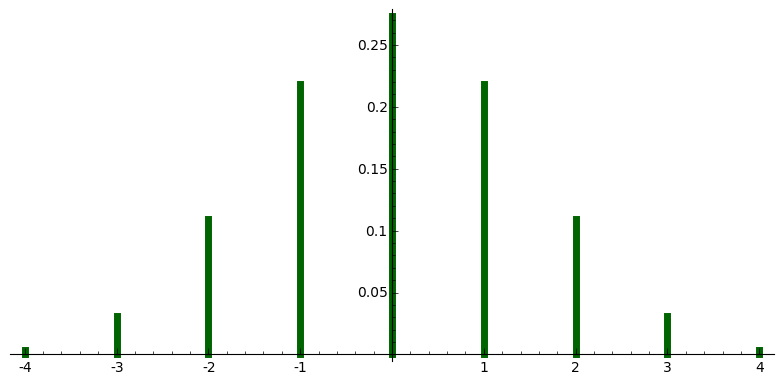
Figure 1: Probability density function of $\mathcal{V}_{8}$

Definition 6

Let $k\geq 2$ be an even integer. Then a sample from the distribution $P_{m,k}$ is

$$e=\sum_{i=0}^{n-1}e_{i}\zeta_{m}^{i},$$

where the coefficients $e_{i}$ are sampled independently from $\mathcal{V}_{k}$.

5.1 Bounding the Distance from Uniform

We recall the definition and key properties of Fourier transform over finite fields. Suppose $f$ is a real-valued function on $\mathbb{F}_{q}$. The Fourier transform of $f$ is defined as

$$\widehat{f}(y)=\sum_{a\in\mathbb{F}_{q}}f(a)\overline{\chi_{y}(a)},$$

where $\chi_{y}(a):=e^{2\pi iay/q}$.

Let $u$ denote the probability density function of the uniform distribution over $\mathbb{F}_{q}$, that is $u(a)=\frac{1}{q}$ for all $a\in\mathbb{F}_{q}$. Let $\delta$ denote the characteristic function of the one-point set $\{0\}\subseteq\mathbb{F}_{q}$. Recall that the convolution of two functions $f,g:\mathbb{F}_{q}\to\mathbb{R}$ is defined as $(f\ast g)(a)=\sum_{b\in\mathbb{F}_{q}}f(a-b)g(b)$. We list without proof some basic properties of the Fourier transform.

1. $\widehat{\delta}=qu$; $\widehat{u}=\delta$.

2. $\widehat{f\ast g}=\widehat{f}\cdot\widehat{g}$.

3. $f(a)=\frac{1}{q}\sum_{y\in\mathbb{F}_{q}}\widehat{f}(y)\chi_{y}(a)$ (the Fourier inversion formula).

The following is a standard result.

Lemma 5

Suppose $F$ and $G$ are independent random variables with values in $\mathbb{F}_{q}$, having probability density functions $f$ and $g$. Then the density function of $F+G$ is equal to $f\ast g$. In general, suppose $F_{1},\ldots,F_{n}$ are mutually independent random variables in $\mathbb{F}_{q}$, with probability density functions $f_{1},\ldots,f_{n}$. Let $f$ denote the density function of the sum $F=\sum F_{i}$, then $f=f_{1}\ast\cdots\ast f_{n}$.

The Fourier transform of $\nu_{k}$ has a nice closed-form formula, as below.

Lemma 6

For all even integers $k\geq 2$, $\widehat{\nu_{k}}(y)=\cos\left(\frac{\pi y}{q}\right)^{k}.$

Proof

We have

$$2^{k}\cdot\widehat{\nu_{k}}(y) =\sum_{m\in\mathbb{Z}/q\mathbb{Z}}\left(\sum_{a\in\mathbb{Z}:|aq+m|\leq k/2}{k\choose aq+m+\frac{k}{2}}\right)e^{-2\pi iym/q}$$

$$=\sum_{m=-\frac{k}{2}}^{\frac{k}{2}}{k\choose m+\frac{k}{2}}e^{2\pi iym/q}$$

$$=e^{-\pi iyk/q}\sum_{m^{\prime}=0}^{k}{k\choose m^{\prime}}e^{2\pi iym^{\prime}/q}$$

$$=e^{-\pi iyk/q}(1+e^{2\pi iy/q})^{k}=(2\cos(\pi y/q))^{k}.$$

Dividing both sides by $2^{k}$ gives the result.

Next, we concentrate on the “reduced distribution” $P_{m,k}\pmod{\mathfrak{q}}$. Note that there is a one-to-one correspondence between primitive $m$-th roots of unity in $\mathbb{F}_{q}$ and the prime ideals above $q$ in $\mathbb{Q}(\zeta_{m})$. Let $\alpha$ be the root corresponding to our choice of $\mathfrak{q}$. Then a sample from $P_{m,k}\pmod{\mathfrak{q}}$ is of the form

$$e_{\alpha}=\sum_{i=0}^{n-1}\alpha^{i}e_{i}\pmod{q},$$

where the coordinates $e_{i}$ are independently sampled from $\mathcal{V}_{k}$. We abuse notations and use $e_{\alpha}$ to denote its own probability density function.

Lemma 7

$$\widehat{e_{\alpha}}(y)=\prod_{i=0}^{n-1}\cos\left(\frac{\alpha^{i}\pi y}{q}\right)^{k}.$$

Proof

This follows directly from Lemma 6 and the independence of the coordinates $e_{i}$.

Lemma 8

Let $f:\mathbb{F}_{q}\to\mathbb{R}$ be a function such that $\sum_{a\in\mathbb{F}_{q}}f(a)=1$. Then for all $a\in\mathbb{F}_{q}$, the following holds.

$$|f(a)-1/q|\leq\frac{1}{q}\sum_{y\in\mathbb{F}_{q},y\neq 0}|\hat{f}(y)|.$$ (1)

Proof

For all $a\in\mathbb{F}_{q}$,

$$f(a)-1/q =f(a)-u(a)$$

$$=\frac{1}{q}\sum_{y\in\mathbb{F}_{q}}(\hat{f}(y)-\widehat{u}(y))\chi_{y}(a)$$

$$=\frac{1}{q}\sum_{y\in\mathbb{F}_{q}}(\hat{f}(y)-\delta(y))\chi_{y}(a)$$

$$=\frac{1}{q}\sum_{y\in\mathbb{F}_{q},y\neq 0}\hat{f}(y)\chi_{y}(a).\qquad\mbox{(since $\hat{f}(0)=1$)}$$

Now the result follows from taking absolute values on both sides, and noting that $|\chi_{y}(a)|\leq 1$ for all $a$ and all $y$.

Taking $f=e_{\alpha}$ in Lemma 8, we immediately obtain

Theorem 5.1

The statistical distance between $e_{\alpha}$ and $u$ satisfies

$$\Delta(e_{\alpha},u)\leq\frac{1}{2}\sum_{y\in\mathbb{F}_{q},y\neq 0}|\widehat{e_{\alpha}}(y)|.$$ (2)

Now let $\epsilon(m,q,k,\alpha)$ denote the right hand side of (2), i.e.,

$$\epsilon(m,q,k,\alpha)=\frac{1}{2}\sum_{y\in\mathbb{F}_{q},y\neq 0}\prod_{i=0}^{n-1}\cos\left(\frac{\alpha^{i}\pi y}{q}\right)^{k}.$$

To take into account all prime ideals above $q$, we let $\alpha$ run through all primitive $m$-th roots of unity in $\mathbb{F}_{q}$ and define

$$\epsilon(m,q,k):=\max\{\epsilon(m,q,k,\alpha):\alpha\mbox{ has order }m\mbox{ in }(\mathbb{F}_{q})^{*}\}.$$

If $\epsilon(m,q,k)$ is negligibly small, then the distribution $P_{m,k}\pmod{\mathfrak{q}}$ will be computationally indistinguishable from uniform. We will prove the following theorem.

Theorem 5.2

Let $q,m$ be positive integers such that $q$ is a prime, $m$ is a power of 2, $q\equiv 1\mod{m}$ and $q<m^{2}$. Let $\beta=\frac{1+\frac{\sqrt{q}}{m}}{2}$; then $0<\beta<1$ and

$$\epsilon(m,q,k)\leq\frac{q-1}{2}\beta^{\frac{km}{4}}.$$

In particular, if $\beta^{k/4}<\frac{1}{2}$, then the theorem says that $\epsilon(m,q,k)=O(q2^{-m})$ as $m\to\infty$.

Corollary 1

The statistical distance between $P_{m,k}$ modulo $\mathfrak{q}$ and a uniform distribution is bounded above, independently of the choice of $\mathfrak{q}$ above $q$, by

$$\frac{q-1}{2}\left(\frac{1+\frac{\sqrt{q}}{m}}{2}\right)^{\frac{km}{4}}.$$

To prepare proving the theorem, we set up some notations of Shparlinski in [18]. Let $\Omega=(\omega_{j})_{j=1}^{\infty}$ be a sequence of real numbers and let $m$ be a positive integer. We define the following quantities:

• $L_{\Omega}(m)=\prod_{j=1}^{m}(1-\exp(2\pi i\omega_{j}))$
  

• $S_{\Omega}(m)=\sum_{j=1}^{m}\exp(2\pi i\omega_{j})$.

The following lemma is a special case of [18, Theorem 2.4].

Lemma 9

$$|L_{\Omega}(m)|\leq 2^{m/2}(1+|S_{\Omega}(m)|/m)^{m/2}.$$

Proof (of Theorem 5.2)

We specialize the above discussion to our situation, where $m$ is a power of 2 and $n=m/2$. We fix $\omega_{k}=\frac{\alpha^{k-1}y}{q}+1/2$, where we abuse notations and let $\alpha$ denote a lift of $\alpha\in\mathbb{F}_{q}$ to $\mathbb{Z}$.

Lemma 10

We have

$$|L_{\Omega}(n)|=2^{n}\left|\prod_{j=0}^{n-1}\cos\left(\frac{\alpha^{j}\pi y}{q}\right)\right|$$

and $|L_{\Omega}(m)|=|L_{\Omega}(n)|^{2}$.

Proof

We have $L_{\Omega}(n)=\prod_{j=1}^{n}(1-e^{2\pi i(\alpha^{j-1}y/q+1/2)})=\prod_{j=0}^{n-1}(1+e^{2\pi i\alpha^{j}y/q})$. So $|L_{\Omega}(n)|=\prod_{j=0}^{n-1}\big{|}e^{-\pi i\alpha^{j}y/q}+e^{\pi i\alpha^{j}y/q)}\big{|}=\prod_{j=0}^{n-1}2\,\big{|}\real(e^{\pi i\alpha^{j}y/q})\big{|}$, which is equal to $2^{n}\big{|}\prod_{j=0}^{n-1}\cos(\alpha^{j}\pi y/q)\big{|}$. Similarly, $|L_{\Omega}(m)|=2^{m}|\prod_{j=0}^{m-1}\cos(\alpha^{j}\pi y/q)|$. Since $\alpha^{n}\equiv-1\mod{q}$ we have $\cos(\alpha^{j+n}\pi y/q)=\cos(\alpha^{j}\pi y/q)$ for $0\leq j\leq n-1$. The claim now follows.

On the other hand, we have $S_{\Omega}(m)=-\sum_{j=0}^{m-1}\exp\left(\frac{2\pi i\alpha^{j}y}{q}\right)$, and standard bound on Gauss sums says that $|S_{\Omega}(m)|\leq q^{1/2}$. Now combining Lemma 9 and Lemma 10, we get

$$\left|\prod_{i=0}^{n-1}\cos\left(\frac{\alpha^{i}\pi y}{q}\right)\right|\leq\beta^{n/2}$$

for $\beta$ as defined in the statement of the theorem and for any nonzero $y\in\mathbb{F}_{q}$. Our result in the theorem now follows from taking both sides to $k$-th power and summing over $y$.

5.2 Numerical Distance from Uniform

We have computed $\epsilon(m,q,k)$ for various choices of parameters. Smaller values of $\epsilon$ imply that the error distribution looks more uniform when transferred to $R/\mathfrak{q}$, rendering the instance of RLWE invulnerable to the attacks in [9].

The data in Table 3 shows that when $n\geq 100$ and the size of the modulus $q$ is polynomial in $n$, the statistical distances between $P_{m,k}\pmod{\mathfrak{q}}$ and the uniform distribution are negligibly small. Also, note that we fixed $k=2$, and the epsilon values becomes even smaller when $k$ increases.

For each instance in Table 3, we also generated the actual RLWE samples (where we fixed $r_{0}=\sqrt{2\pi}$) and ran the chi-square attack of [9] using confidence level $\alpha=0.99$. The column labeled “$\chi^{2}$” contains the $\chi^{2}$ values we obtained, and the column labeled “uniform?” indicates whether the reduced errors are uniform. We can see from the data how the practical situation agrees with our analysis on the approximated distributions.

Table 3: Values of $\epsilon(m,q,2)$ and the $\chi^{2}$ values

$m$ ($n=m/2$)	$q$	$-[\log_{2}(\epsilon(m,q,2))]$	$\chi^{2}$	uniform?
64	193	40	167.6	yes
128	1153	97	1125.6	yes
256	3329	$194$	3350.0	yes
512	10753	431	10732.8	yes

It is possible to generalize our discussion in this section to primes of arbitrary residue degree $f$, in which case the Fourier analysis will be performed over the field $\mathbb{F}_{q^{f}}$. The only change in the definitions would be $\chi_{y}(a)=e^{\frac{2\pi i\Tr(ay)}{q}}$. Here $\Tr:\mathbb{F}_{q^{f}}\to\mathbb{F}_{q}$ is the trace function. Similarly, we have

$$\widehat{e^{\prime}_{\alpha}}(y)=\prod_{i=1}^{n}\cos\left(\frac{\pi\Tr(\alpha^{i}y)}{q}\right)^{k}.$$

Table 4 contains some data for primes of degree two.

Table 4: Values of $\epsilon(m,q,2)$ for primes of degree two

$m$ ($n=m/2$)	$q$	$-[\log_{2}(\epsilon(m,q,2))]$
64	383	31
128	1151	54
256	1279	159
512	5583	341

References

- [1] Ajtai, M., Dwork, C.: A public-key cryptosystem with worst-case/average-case equivalence. In: Proceedings of the twenty-ninth annual ACM symposium on Theory of computing. pp. 284–293. ACM (1997)
- [2] Bos, J.W., Lauter, K., Loftus, J., Naehrig, M.: Improved security for a ring-based fully homomorphic encryption scheme. In: Cryptography and Coding, pp. 45–64. Springer (2013)
- [3] Brakerski, Z.: Fully homomorphic encryption without modulus switching from classical GapSVP. In: Advances in Cryptology–CRYPTO 2012, pp. 868–886. Springer (2012)
- [4] Brakerski, Z., Gentry, C., Vaikuntanathan, V.: (Leveled) fully homomorphic encryption without bootstrapping. In: Proceedings of the 3rd Innovations in Theoretical Computer Science Conference. pp. 309–325. ACM (2012)
- [5] Brakerski, Z., Vaikuntanathan, V.: Fully homomorphic encryption from Ring-LWE and security for key dependent messages. In: Advances in Cryptology–CRYPTO 2011, pp. 505–524. Springer (2011)
- [6] Brakerski, Z., Vaikuntanathan, V.: Efficient fully homomorphic encryption from (standard) LWE. SIAM Journal on Computing 43(2), 831–871 (2014)
- [7] Castryck, W., Iliashenko, I., Vercauteren, F.: On error distributions in Ring-based LWE. Cryptology ePrint Archive, Report 2016/240 (2016), http://eprint.iacr.org/2016/240
- [8] Castryck, W., Iliashenko, I., Vercauteren, F.: Provably weak instances of Ring-LWE revisited. In: Annual International Conference on the Theory and Applications of Cryptographic Techniques. pp. 147–167. Springer (2016)
- [9] Chen, H., Lauter, K., Stange, K.E.: Attacks on search-RLWE. Cryptology ePrint Archive, Report 2015/971 (2015), http://eprint.iacr.org/
- [10] Eisenträger, K., Hallgren, S., Lauter, K.: Weak instances of PLWE. In: Selected Areas in Cryptography–SAC 2014, pp. 183–194. Springer (2014)
- [11] Elias, Y., Lauter, K., Ozman, E., Stange, K.: Provably weak instances of Ring-LWE. In: Advances in Cryptology – CRYPTO 2015, Lecture Notes in Comput. Sci., vol. 9215, pp. 63–92. Springer, Heidelberg (2015)
- [12] Hoffstein, J., Pipher, J., Silverman, J.H.: An introduction to mathematical cryptography, vol. 1. Springer (2008)
- [13] López-Alt, A., Tromer, E., Vaikuntanathan, V.: On-the-fly multiparty computation on the cloud via multikey fully homomorphic encryption. In: Proceedings of the forty-fourth annual ACM symposium on Theory of computing. pp. 1219–1234. ACM (2012)
- [14] Lyubashevsky, V., Peikert, C., Regev, O.: On ideal lattices and learning with errors over rings. Journal of the ACM (JACM) 60(6), 43 (2013)
- [15] Marcus, D.A.: Number fields, vol. 18. Springer (1977)
- [16] Micciancio, D., Regev, O.: Worst-case to average-case reductions based on Gaussian measures. SIAM Journal on Computing 37(1), 267–302 (2007)
- [17] Regev, O.: On lattices, learning with errors, random linear codes, and cryptography. Journal of the ACM (JACM) 56(6), 34 (2009)
- [18] Shparlinski, I.E.: On some characteristics of uniformity of distribution and their applications. In: Computational Algebra and Number Theory, pp. 227–241. Springer (1995)
- [19] Stehlé, D., Steinfeld, R.: Making NTRU as secure as worst-case problems over ideal lattices. In: Advances in Cryptology–EUROCRYPT 2011, pp. 27–47. Springer (2011)