A quantum mechanical well and a derivation of a $\pi^{2}$ formula.

Abstract

Quantum particle bound in an infinite, one-dimensional square potential well is one of the problems in Quantum Mechanics (QM) that most of the textbooks start from. There, calculating an allowed energy spectrum for an arbitrary wave function often involves Riemann zeta function resulting in a $\pi$ series griffits-1 . In this work, two “$\pi$ formulas” are derived when calculating a spectrum of possible outcomes of the momentum measurement for a particle confined in such a well, the series, $\frac{\pi^{2}}{8}=\sum_{k=1}^{k=\infty}\frac{1}{(2k-1)^{2}}$, and the integral $\int_{-\infty}^{\infty}\frac{sin^{2}x}{x^{2}}dx=\pi$. The spectrum of the momentum operator appears to peak on classically allowed momentum values only for the states with even quantum number. The present article is inspired by another quantum mechanical derivation of $\pi$ formula in wallys .

The $\pi^{2}$ series :

$$\frac{\pi^{2}}{8}=\sum_{k=1}^{k=\infty}\frac{1}{(2k-1)^{2}}=1+\frac{1}{3^{2}}+\frac{1}{5^{2}}...$$ (1)

cited for example in numbers and wolfram is not attracting much attention, perhaps due to its relatively slow convergence. The integral $\int_{-\infty}^{\infty}\frac{sin^{2}x}{x^{2}}dx=\pi$ can be calculated using complex number analysis. As shown here, both of these have to be true to ensure the consistency of QM formalism when calculating the spectrum of possible outcomes of the momentum measurement for a quantum particle in a one-dimensional (1D) infinite square well. The derivation involves Fourier series and Fourier transform. The momentum operator spectrum appears to be different than naively expected. A derivation of the Wallis formula for $\pi$ in the context of QM analysis of hydrogen atom was demonstrated in wallys .

It is a fundamental assumption of QM, that most of textbooks start from that all information about a system at a given instant of time can be derived from the wave function mandl1.1 , $\Psi(\vec{r},t)$. Hermitian operators representing the measurable quantities (observables) provide the way of deriving this information. While the average result of a measurement obtained on an ensemble of identically prepared systems can be calculated as an expectation value of an operator in question, $\hat{O}$,

$$<\hat{O}>=\int\Psi^{*}(\vec{r},t)\hat{O}\Psi(\vec{r},t)d^{3}r$$ (2)

the outcomes of single measurements are eigenvalues of this operator. The link between the eigenvalues and the expectation values is provided by the formulas below. For a discrete spectrum of eigenvalues, $o_{k}$, one gets,

$$<\hat{O}>=\Sigma_{k}|c_{k}|^{2}o_{k}$$ (3)

whereas the sum is replaced by an integral in case of a continuous spectrum of eigenvalues, $k$,

$$<\hat{O}>=\int|c(k)|^{2}kdk$$ (4)

The modulus squared of a coefficient $|c_{k}|^{2}$ (the function $|c(k)|^{2}dk$ ) represent the probability to measure a given eigenvalue $o_{k}$ (an eigenvalue between $k$ and $k+dk$) in case of a discrete (continuous) spectrum of eigenvalues. These coefficients can be calculated when representing the wave function of the system as a linear combination of the orthonormal eigenfunctions of the operator in question.

One typical QM exercise illustrating the above mechanism is to represent an eigenfunction the Hamiltonian , $\Psi(\vec{r})$, as a linear combination of orthonormal eigenfunctions, $\Phi_{k}(\vec{r})$, of another observable of interest, $\Psi(\vec{r})=\Sigma_{k}c_{k}\Phi_{k}(\vec{r})$ (or $\Psi(\vec{r})=\int c(k)\Phi_{k}(\vec{r})dk$ for continuous spectrum) in order to calculate what are the possible outcomes of the measurements of this observable for a state with a well defined energy (a stationary state). An expansion coefficient $c_{\xi}$ or a function $c(\xi)$ can be calculated as a scalar product of $\Phi^{*}_{\xi}$ and $\Psi(\vec{r})$:

$$c(\xi)=\int\Phi^{*}_{\xi}(\vec{r})\Psi(\vec{r})d^{3}r~{}~{}\text{or}~{}~{}c_{\xi}=\int\Phi^{*}_{\xi}(\vec{r})\Psi(\vec{r})d^{3}r\\$$ (5)

This exercise, performed below for the imaginably simplest QM system with an endeavor to calculate the possible outcomes of momentum measurement, yields a somewhat unexpected conclusion.

The eigenfunctions of the Hamiltonian,

$$\hat{H}=-\frac{\hbar^{2}}{2m}\frac{d^{2}}{dx^{2}}+V(x)$$ (6)

inside an infinite one-dimensional square well situated in $0\leq x\leq L$ can be found in any QM textbook griffith-2 and are of the form:

$$\Psi_{n}(x)=\sqrt{\frac{2}{L}}sin(\frac{x}{L}n\pi)$$ (7)

These functions are orthonormal inside the well $0\leq x\leq L$ and form a complete set. They fulfill correct boundary conditions, disappearing at the borders of the well since the wave function has to be continuous and cannot exist in the area of the infinite potential. They also give the known energy spectrum,

$$E_{n}=\frac{1}{2m}(\frac{n\pi\hbar}{L})^{2}=\frac{<p_{x}^{2}>}{2m}$$ (8)

However, they are not eigenfunctions of the 1D momentum operator, $\hat{p_{x}}\equiv\frac{\hbar}{i}\frac{d}{dx}$. A classical particle bound in the well with the kinetic energy $E_{n}$ would be bouncing back and forth with the momentum $p_{x}=\pm\frac{n\pi\hbar}{L}$. A quantum particle has $<\hat{p}^{2l+1}_{x}>=0$ and $<\hat{p}^{2l}_{x}>=(\frac{n\pi\hbar}{L})^{2l}$ as can be easily calculated using space representation of the $\hat{p_{x}}$ and the Hamiltonian eigenfunctions with use of the formula 2.

In order to calculate the possible outcomes of momentum measurements one has to use an orthonormal and complete set of the momentum operator eigenfunctions. The usual procedure is to propose the eigenfunctions with either a continuous spectrum of eigenvalues, as suggested in griffithp22 , normalized to the Dirac $\delta$ or with a discrete spectrum of eigenvalues, normalized inside the well and fulfilling the periodic boundary conditions mandl-momentum .

For example, $\Phi_{k}(x)=\frac{1}{\sqrt{2\pi}}exp({ikx})$ is a continuous spectrum eigenfunction of ${\hat{p_{x}}/\hbar}$ normalized as follows, $\int_{-\infty}^{\infty}\Phi_{k}(x)\Phi_{k}^{\prime}(x)dx=\delta({k-k^{\prime}})$.

For the discrete spectrum, the orthonormal set of momentum eigenfunctions normalized inside the well, $\Xi(x)=\frac{1}{\sqrt{L}}exp({\frac{ipx}{\hbar}})$, needs to fulfill the periodic boundary conditions, $\Xi(L)=\Xi(0)$. These conditions:

$$\frac{1}{\sqrt{L}}exp({\frac{ipL}{\hbar}})=\frac{1}{\sqrt{L}}\\$$ (9)

result in:

$$exp({\frac{ipL}{\hbar}})=1,~{}\frac{pL}{\hbar}=2l\pi,\\$$ (10)

where $l$ is an integer number.

Denoting the momentum eigenfunctions with positive and negative $l$ as follows:

$$\Xi^{+}_{n}(x)=\frac{1}{\sqrt{L}}exp({\frac{+i2n\pi x}{L}})~{},~{}~{}~{}~{}\Xi^{-}_{n}(x)=\frac{1}{\sqrt{L}}exp({\frac{-i2n\pi x}{L}})\\$$ (11)

one has now $n$ a natural number, or zero. For $n=0$ one gets , $\Xi_{0}(x)=\frac{1}{\sqrt{L}}$ with zero eigenvalue.

The momentum operator eigenvalues are thus of the form: ${\frac{2n\pi\hbar}{L}}$, different than naively expected, eigenvalues which are odd number multiplications of ${\frac{\pi\hbar}{L}}$ being absent. Since these eigenvalues can in principle be measured the question of what is the momentum operator spectrum is not purely academic one. For completeness, the orthonormality of the functions $\Xi^{\pm}_{n}(x)$ is shown in the Appendix A2.

Probabilities to measure given $p_{x}$ values are calculated below and compared for continuous and discrete spectra. The probability, $P_{n}(k)dk=|c_{n}(k)|^{2}dk$ to measure a given value of $k$, $p_{x}=\hbar k$, for a given state $\Psi_{n}(x)$ of the particle in the well, using the continuous spectrum momentum eigenfunctions can be calculated as follows,

$$c_{n}(k)=\int_{0}^{L}\Phi^{*}_{k}(x^{\prime})\Psi_{n}(x^{\prime})dx^{\prime}=\frac{1}{\sqrt{2\pi}}\sqrt{\frac{2}{L}}\int_{0}^{L}exp({-ikx})sin(\frac{n\pi x}{L})dx\\$$ (12)

$$P_{n}(k)=|c_{n}(k)|^{2}=\frac{n^{2}\pi L}{(L\cdot k+n\pi)^{2}(L\cdot k-n\pi)^{2}}|(-1)^{n}exp(iLk)-1|^{2}\\$$ (13)

Since $|(-1)^{n}exp(iLk)-1|^{2}=4cos^{2}(Lk/2)$ for odd $n$ and $|(-1)^{n}exp(iLk)-1|^{2}=4sin^{2}(Lk/2)$ for even $n$ one gets a somewhat surprising result that the probability to measure a certain momentum $p_{x}=\hbar k$ peaks at the classical momentum values $p_{x}=\hbar k=\pm\frac{n\hbar\pi}{L}$ only for even $n$ values, whereas for odd $n$ values it peaks up at $p_{x}=0$. Figure 1 shows the probability density as a function of a dimensionless variable, $\xi=kL=\frac{p_{x}L}{\hbar}$ proportional to the momentum eigenvalue, for the ground state ($n=1$) and the first excited state ($n=2$) of the well. The expectation value of the momentum operator is zero, since the probability density in formula 13 is a symmetric function. For this momentum space wave function to be correctly normalized and to give the correct expectation value of$<\hat{p}^{2}_{x}>=(\frac{n\pi\hbar}{L})^{2}$ the following must hold (for $n=1$):

$$\int_{-\infty}^{\infty}|c_{1}(\xi=kL)|^{2}d\xi=\int_{-\infty}^{\infty}\frac{4\pi}{(\xi+\pi)^{2}(\xi-\pi)^{2}}cos^{2}(\xi/2)d\xi=1\\$$ (14)

$$\int_{-\infty}^{\infty}|c_{1}(\xi=kL)|^{2}\xi^{2}d\xi=\int_{-\infty}^{\infty}\frac{4\pi}{(\xi+\pi)^{2}(\xi-\pi)^{2}}cos^{2}(\xi/2)\xi^{2}d\xi=\pi^{2}\\$$ (15)

These integrals are equivalent to $\int_{-\infty}^{\infty}\frac{sin^{2}x}{x^{2}}dx=\pi$, see the Appendix A1 for the algebra. Note that it is not possible to sensibly calculate the expectation value of the higher powers, $<\hat{p}^{2l}_{x}>$, of the momentum operator using the momentum space wave function $c_{n}(k)$, the integral is divergent already for $l=2$.

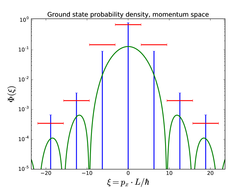
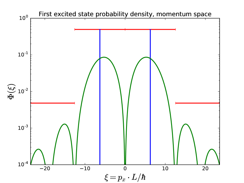
Figure 1: Probability density (green line) and discrete probabilities (blue columns) to measure a given momentum value for the ground state, left, and the first excited state, right, for a particle in a one dimensional infinite well of the size $L$. Red bars show values of integrals of the probability density in the range of the bar.

The possible spectrum of outcomes of momentum measurements for a particle in the ground state and the first excited state is obtained below using the momentum operator eigenfunctions with the discrete spectrum. Here one needs to express the eigenfunctions of the Hamiltonian mandl2 , $\Psi_{1}(x)=\sqrt{\frac{2}{L}}sin(\frac{\pi x}{L})$ and $\Psi_{2}(x)=\sqrt{\frac{2}{L}}sin(\frac{2\pi x}{L})$, as a combination of momentum operator eigenfunctions in formula 11.

Finding the expansion coefficients for the first excited state eigenfunction in the well is straightforward because $\Psi_{2}(x)$ is a simple combination of $\Xi^{+}_{1}=\frac{1}{\sqrt{L}}exp({\frac{+i2\pi x}{L}})$ and $\Xi^{-}_{1}=\frac{1}{\sqrt{L}}exp({\frac{-i2\pi x}{L}})$, $\Psi_{2}(x)=\frac{i}{\sqrt{2}}(\Xi^{-}_{1}-\Xi^{+}_{1})$. Thus there are two possible results of the momentum measurement, $p_{x}=\frac{2\pi\hbar}{L}$ and $p_{x}=-\frac{2\pi\hbar}{L}$, occurring with equal probabilities, resulting in the $<\hat{p_{x}}>=0$, in agreement with the classical result.

The result for the ground state wave function $\Psi_{1}(x)=\sqrt{\frac{2}{L}}sin(\frac{\pi x}{L})$ is more involved. The expansion coefficients can be calculated using the formula 5:

$$\Psi(x)=\Sigma_{i}{c_{i}\Xi_{i}(x)}~{},~{}~{}c_{n}=\int_{0}^{L}\Xi^{*}_{n}(x^{\prime})\Psi(x^{\prime})dx^{\prime}\\$$ (16)

For the ground state wave function $\Psi_{1}(x)=\sqrt{\frac{2}{L}}sin(\frac{x\pi}{L})$, the expansion coefficients are:

$$c_{\pm k}=\int_{0}^{L}\Xi^{*}_{\pm k}(x^{\prime})\sqrt{\frac{2}{L}}sin(\frac{x^{\prime}\pi}{L})dx^{\prime}\\$$ (17)

$$c_{\pm k}=\frac{\sqrt{2}}{2i}\left[\frac{exp{(\frac{i(\mp 2k+1)\pi x^{\prime}}{L}})}{i\pi(\mp 2k+1)}-\frac{exp{(\frac{i(\mp 2k-1)x^{\prime}\pi}{L}})}{i\pi(\mp 2k-1)}\right]_{0}^{L}$$ (18)

Since both, $\mp 2k+1$, and, $\mp 2k-1$, are odd numbers both exponential functions are $=-1$ for $x^{\prime}=L$. One gets:

$$c_{+k}=-\frac{1}{\pi}\cdot\frac{2\sqrt{2}}{(2k-1)(2k+1)}=c_{-k}$$ (19)

The modulus squared of a given coefficient defines the probability to measure a given momentum value in the ground state of the infinite square well:

$$|c_{\pm k}|^{2}=\frac{1}{\pi^{2}}\cdot\frac{8}{(2k-1)^{2}(2k+1)^{2}}$$ (20)

All the coefficients are non-zero, thus the whole spectrum of the momentum operator eigenvalues can be measured for a particle in the ground state of the infinite square well. Figure 1 shows the numerical values of some of these coefficients compared with the probability density in formula 14 calculated using the continuous spectrum of momentum eigenvalues, for the ground state and the first excited state of the well. In the ground state, the largest probability is to measure null momentum, the same conclusion was reached using the momentum eigenfunction with the continuous spectrum of eigenvalues. Again, as expected, $<\hat{p_{x}}>=0$.

The moduli squared of all coefficients in formula 20 must sum up to unity, since they together represent the probability of measuring any momentum value. Thus:

$$|c_{0}|^{2}+2\cdot\sum_{1}^{\infty}|c_{k}|^{2}=\frac{8}{\pi^{2}}+\frac{2}{\pi^{2}}\cdot\sum_{1}^{\infty}\frac{8}{(2k-1)^{2}(2k+1)^{2}}=1$$ (21)

This implies the following relation involving $\pi^{2}$ to be true, identical to the equation 32 in Appendix A1:

$$\frac{1}{2}+\sum_{1}^{\infty}\frac{1}{(2k-1)^{2}(2k+1)^{2}}=\frac{\pi^{2}}{16}$$ (22)

The eigenvalues of the Hamiltonian, $\hat{H}=\frac{\hat{p}^{2}}{2m}$ for the particle in the well are given in the formula 8. The expectation value of the Hamiltonian on the ground state eigenfunction, $\Psi_{1}(x)=\sqrt{\frac{2}{L}}sin(\frac{x\pi}{L})$, is equal to $E_{1}$. If one calculates the expectation value of $\hat{H}$ in 6 using the expansion in formula 16 one gets:

$$E_{1}=<\hat{H}>=2*\sum_{1}^{\infty}(2k)^{2}E_{1}\cdot\frac{1}{\pi^{2}}\cdot\frac{8}{(2k-1)^{2}(2k+1)^{2}}\\$$ (23)

Thus another relation involving $\pi^{2}$ in 31 in Appendix A1 has to be fulfilled :

$$\sum_{1}^{\infty}\frac{(2k)^{2}}{(2k-1)^{2}(2k+1)^{2}}=\frac{\pi^{2}}{16}$$ (24)

The formulas in 22 and in 24 are trivially equivalent to each other and to the known $\pi^{2}$ series in the formula 1, see Appendix A1. It has been thus demonstrated that $\pi^{2}$ formula in 1 stems from the spectrum of possible outcomes of momentum measurements for a QM particle confined in a one-dimensional box. The continuous and discrete spectra of momentum eigenvalues show similar features peaking at $p_{x}=0$ for the ground state (and any odd $n$) and at the classically allowed momentum values for the first excited state (any even $n$). The second power of momentum operator is the highest even power the expectation value of which can be sensibly calculated with the momentum representation of the infinite well wave function, both in its continuous $c(k)$ or discrete $c_{k}$ form.

I Acknowledments

We thank Per Osland for cross-checking the formulas and pertinent comments on the presentations of these results.

II Appendix A1

The equations 14 and 15 can be rewritten as follows:

$$\int_{-\infty}^{\infty}\frac{4}{(z+1)^{2}(z-1)^{2}}cos^{2}(z\pi/2)dz=\pi^{2}\\$$ (25)

$$\int_{-\infty}^{\infty}\frac{4}{(z+1)^{2}(z-1)^{2}}cos^{2}(z\pi/2)z^{2}dz=\pi^{2}\\$$ (26)

Adding them and dividing by two one obtains:

$$\int_{-\infty}^{\infty}(\frac{1}{(z+1)^{2}}+\frac{1}{(z-1)^{2}})cos^{2}(z\pi/2)dz=\pi^{2}\\$$ (27)

or, after elementary integration variable changes:

$$\int_{-\infty}^{\infty}\frac{cos^{2}(y\pi/2-\pi/2)}{y^{2}}dy+\int_{-\infty}^{\infty}\frac{cos^{2}(y\pi/2+\pi/2)}{y^{2}}dy=\pi^{2}\\$$ (28)

$$2\int_{-\infty}^{\infty}\frac{sin^{2}(y\pi/2)}{y^{2}}dy=\pi^{2}\\$$ (29)

$$\int_{-\infty}^{\infty}\frac{sin^{2}(x)}{x^{2}}dx=\pi\\$$ (30)

A simple rearrangement of the equation 1 leads to the two formulas below:

$$SUM1\equiv\sum_{1}^{\infty}\frac{(2k)^{2}}{(2k-1)^{2}(2k+1)^{2}}=\frac{\pi^{2}}{16}$$ (31)

and,

$$\frac{1}{2}+SUM2\equiv\frac{1}{2}+\sum_{1}^{\infty}\frac{1}{(2k-1)^{2}(2k+1)^{2}}=\frac{\pi^{2}}{16}\\$$ (32)

The equations 31, 32 are trivially equivalent as it can be readily noted by subtracting the two series above:

$$SUM1-SUM2=\sum_{1}^{\infty}\frac{(2k)^{2}-1}{(2k-1)^{2}(2k+1)^{2}}=\sum_{1}^{\infty}\frac{1}{(2k-1)(2k+1)}=\frac{1}{2}[\sum_{1}^{\infty}\frac{1}{(2k-1)}-\sum_{1}^{\infty}\frac{1}{(2k+1)}]=\frac{1}{2}\\$$ (33)

Further, it follows from formula 1,

$$\frac{\pi^{2}}{4}=1+\sum_{k=1}^{k=\infty}\frac{1}{(2k+1)^{2}}+\sum_{k=1}^{k=\infty}\frac{1}{(2k-1)^{2}}=1+\sum_{k=1}^{k=\infty}\frac{(8k^{2}+2)}{(2k-1)^{2}(2k+1)^{2}}=1+2\cdot SUM1+2\cdot SUM2=4\cdot SUM1\\$$ (34)

Thus indeed the formula 1 is equivalent to $4\cdot SUM1=\frac{\pi^{2}}{4}$ and, in consequence, to the formulas 31 and 32:

III Appendix A2

The functions of the form:

$$\Phi^{+}_{n}(x)=\frac{i}{\sqrt{L}}exp({\frac{+in\pi x}{L}}),\Phi^{-}_{n}(x)=\frac{i}{\sqrt{L}}exp({\frac{-in\pi x}{L}})\\$$ (35)

are eigenfunctions of the momentum operator, but they do not form an orthonormal set. The usual procedure is to propose an orthonormal set of momentum eigenfunctions normalized in the well, $\Xi(x)=\frac{1}{\sqrt{L}}exp({\frac{ipx}{\hbar}})$, which fulfill periodic boundary conditions, $\Xi(L)=\Xi(0)$.

These momentum operator eigenfunctions are indeed orthonormal in the range $[0,L]$ as basic explicit calculation shows:

$\int_{0}^{L}(\Xi^{+}_{n}(x))^{*}\Xi^{+}_{m}(x)dx=\frac{1}{{L}}\int_{0}^{L}exp({\frac{-i2n\pi x}{L}})exp({\frac{i2m\pi x}{L}})dx$

for $m\neg n$ one has:

$\frac{1}{{L}}\int_{0}^{L}exp({\frac{-i2n\pi x}{L}})exp({\frac{i2m\pi x}{L}})dx=\frac{1}{i2(m-n)\pi}[exp({i2(m-n)\pi})-1]=0$

for $m=n$ one gets $1$. Functions with minus sign are complex-conjugates of the functions with the sign, $(+)$, thus the orthonormality is also valid for them. The scalar product of functions with different signs should always give zero:

$\int_{0}^{L}(\Xi^{-}_{n}(x))^{*}\Xi^{+}_{m}(x)dx=\frac{1}{{L}}\int_{0}^{L}exp({\frac{i2n\pi x}{L}})exp({\frac{i2m\pi x}{L}})dx$

$\frac{1}{{L}}\int_{0}^{L}exp({\frac{i2n\pi x}{L}})exp({\frac{i2m\pi x}{L}})dx=\frac{1}{i2(m+n)\pi}[exp({i2(m+n)\pi})-1]=0$

References

(1)
see for example David J, Griffiths, Introduction
to Quantum Mechanics, Second Edition, ISBN 10:1-292-02408-9, Chapter 2, part 2, example 3
(2)Tamar Friedman and C.R. Hagen, “Quantum mechanical derivation of the Wallis formula for ”, Journal of Mathematical Physics 56, 112101 (2015); doi: 10.1063/1.4930800
(3)David Wells, The Penguin Dictionary of Curious and Interesting Numbers (Penguin Press Science) ISBN:987-0-14-192940-8
(4) see for example F. Mandl, Quantum Mechanics, Manchester Physics Series,
ISBN 0-471-93155-1, Chapter 1.1.