Solitons in a Hamiltonian ${\cal PT}$-symmetric coupler

Abstract

We introduce a nonlinear parity-time-symmetric dispersive coupler which admits Hamiltonian and Lagrangian formulations. We show that, in spite of the gain and dissipation, the model has several conservation laws. The system also supports a variety of exact solutions. We focus on exact bright solitons and demonstrate numerically that they are dynamically stable in a wide parameter range and undergo elastic interactions, thus manifesting nearly-integrable dynamics. Physical applications of the introduced model in the theory of Bose-Einstein condensates in nonlinear lattices are discussed.

1 Introduction

The relation between Hermitian quantum mechanics and its parity-time (${\cal PT}$–) symmetric extension became the focus of intense debates shortly after the latter paradigm was introduced in [1]. In particular, it was shown that any ${\cal PT}$-symmetric Hamiltonian with purely real spectrum, i.e., in the unbroken ${\cal PT}$-symmetric phase, can be transformed to a Hermitian one using a similarity transformation [2]. This fact establishes certain equivalence between the two formulations. In the classical limit, ${\cal PT}$-symmetric models occupy an “intermediate position” between conservative and dissipative nonlinear systems, featuring properties of both these types (see the discussion in [3]). A typical real-world ${\cal PT}$-symmetric system consists of an active element coupled to a lossy one, like those theoretically introduced [4] and experimentally studied [5] in the non-Hermitian discrete optics. Generally, gain and dissipation break the conservation laws for energy or other physically relevant quantities. This strongly affects the nonlinear dynamics, making impossible (or highly nontrivial) its description using the analytical approaches, available, say, for Hamiltonian systems.

Recently, it has been discovered that dynamics of some nonlinear ${\cal PT}$-symmetric models with gain and dissipation still can be described using the Hamiltonian formalism and is therefore characterized by a rather high degree of regularity. More specifically, the Hamiltonian structure has been revealed for ${\cal PT}$-symmetric coupled oscillators [6], for some completely integrable dimer models [7, 8, 9, 10, 11, 12], and for chains of ${\cal PT}$-symmetric pendula [13]. We also mention that systems which do not posses ${\cal PT}$ symmetry but display characteristics of conservative and dissipative ones, are also known; they are described by time-reversible Hamiltonians [14]. However, all the mentioned examples belong to the class of dynamical systems, i.e., the corresponding models are described by systems of ordinary differential equations.

The main goal of this paper is to introduce a nonlinear ${\cal PT}$-symmetric dispersive system which incorporates gain and losses and at the same time allows for the Hamiltonian formulation. This model emerges as a ${\cal PT}$-generalization of the resonant four-wave mixing process in a spinor Bose-Einstein condensate loaded in linear and nonlinear lattices. We demonstrate that such a two-component model, where one component experiences gain and another one loses atoms, can be obtained from a real-valued Hamiltonian. Next, we explore the associated conserved quantities and present various exact solutions and some traits of the system’s nonlinear dynamics. We in particular focus on exact bright soliton solutions and demonstrate numerically that they are stable in a wide parameter range.

The paper is organized as follows. In Sec. 2 we discuss a physical example where the proposed ${\cal PT}$-symmetric model arises. The model itself and its basic properties are presented in Sec. 3. Section 4 demonstrates that the introduced system admits a variety of exact solutions which can be written down in the analytical form, and Sec. 5 studies exact solutions in the form of bright solitons. Finally, Sec. 6 concludes the paper and outlines some perspectives.

2 On the physical model

To introduce the model, we start with a physical example. We consider a one-dimensional Bose-Einstein condensate (BEC) loaded in a linear lattice which experimentally can be created by a two counter-propagating laser beams [15]. We also assume that the scattering length varies periodically in space, i.e. creates a nonlinear lattice. The latter can be created, for example, by periodically varying external field affecting the scattering length by means of the Feshbach resonance. Nonlinear lattices have been realized in laboratory [16] and studied in numerous theoretical works (see e.g. Refs. [17, 18]). In particular, in [18] it was shown that matching condition for resonant four-wave processes can be achieved by modification the momentum, while in the linear lattices the matching condition is achieved by the modifying the dispersion relation  [19].

The meanfield Hamiltonian describing the BEC in linear and nonlinear lattices reads

$$\hat{H}_{\rm BEC}=\int_{-\infty}^{\infty}\left\{{\Psi}^{*}\hat{h}{\Psi}+\tilde{\Omega}\cos(\nu t)V_{1}(x)|\Psi|^{2}+\chi(x)[1+2\cos(2\nu t)]|\Psi|^{4}\right\}dx,$$ (1)

where $\Psi$ is an order parameter $\hat{h}=-\partial_{x}^{2}+V_{0}(x)$, $V_{0,1}(x)=V_{0,1}(x+L)$ are the even (”$0$”) and odd (”$1$”) components of the optical lattice: $V_{0}(x)=V_{0}(-x)$, $V_{1}(x)$ and $V_{1}(x)=-V_{1}(-x)$, $L$ is the lattice period, $\tilde{\Omega}\ll 1$ is the small parameter defining relative depth of the odd component, and $\chi(x)=\chi(x+L)$ describes the nonlinear lattice which undergoes periodic oscillations with the frequency $2\nu$. The value of $\nu$ will be specified below. The amplitude of the shallow odd lattice $V_{1}(x)$ also periodically varies in time but with the frequency $\nu$. In (1) dimensionless units with $\hbar=1$ and $m=1/2$, where $m$ is the atomic mass, are used.

Let us consider the evolution of a superposition $\Psi=\Psi_{1}(x,t)+\Psi_{2}(x,t)$ of two wave packets of Bloch states. Choosing these states as shown in Fig. 1, i.e. Bloch modes with zero group velocities and having energies at the band edges with equal signs of curvatures of the dispersion relations, one can look for a solution in the form

$$\begin{array}[]{l}\displaystyle{\Psi_{1}(x,t)=\left[\epsilon u(\tilde{x},\tilde{t})\psi_{1}(x)+\epsilon^{2}\frac{\partial u}{\partial\tilde{x}}\tilde{\psi}_{1}(x)+\cdots\right]e^{-i{\cal E}_{1}t},}\\[8.53581pt] \displaystyle{\Psi_{2}(x,t)=\left[\epsilon v(\tilde{x},\tilde{t})\psi_{2}(x)+\epsilon^{2}\frac{\partial v}{\partial\tilde{x}}\tilde{\psi}_{2}(x)+\cdots\right]e^{-i{\cal E}_{2}t}.}\end{array}$$ (4)

Here $\epsilon\ll 1$ is a formal small parameter, $u(\tilde{x},\tilde{t})$ and $v(\tilde{x},\tilde{t})$ are functions of slow variables $\tilde{x}=\epsilon x$ and $\tilde{t}=\epsilon^{2}t$, i.e., envelopes of the Bloch states $\psi_{1,2}$ corresponding to the energies ${\cal E}_{1,2}$: $\hat{h}\psi_{j}={\cal E}_{j}\psi_{j}$ ($j=1,2$). In this case, $\psi_{1}$ and $\psi_{2}$ are real-valued periodic functions, as it follows from the Floquet theorem). Detailed calculations of other functional coefficients of the expansions (4), i.e., functions $\tilde{\psi}_{1,2}(x)$ can be performed within the framework of the multiple scale analysis. Here we do not present all the details as they are available in the literature (see e.g. [20]), but only show their effect on the Hamiltonian structure of the model. In the meantime, it will be important that $\psi_{j}$ and $\tilde{\psi}_{j}$ are orthogonal to each other, which in our case means that $\int_{-L/2}^{L/2}\psi_{j}(x)\tilde{\psi}_{j}(x)dx=0$. Thus the dynamics of the superposition $\Psi$ is completely determined by the evolution of $u(\tilde{x},\tilde{t})$ and $v(\tilde{x},\tilde{t})$, and our aim is to obtain the Hamiltonian of this dynamics.

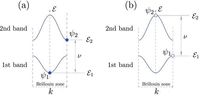
Figure 1: Two schematic representations of resonantly interacting pairs of Bloch modes in the linear lattice. Panels (a) and (b) correspond to two pairs of modes (shown with circles) with positive and negative curvatures of dispersion relations (i.e., effective masses), respectively. In both panels, $k$ is the Bloch momentum.

Now we use substitution (4) in the Hamiltonian (1) and require $\nu$ to be the difference between the energies of the states: $\nu={\cal E}_{2}-{\cal E}_{1}$ (see Fig. 1). The formulated assumptions allow to approximate different terms as follows:

$$\int_{-\infty}^{\infty}{\Psi}^{*}\hat{h}{\Psi}dx\approx\epsilon^{2}\int_{-\infty}^{\infty}\left({\cal E}_{1}\psi_{1}^{2}|u|^{2}+{\cal E}_{2}\psi_{2}^{2}|v|^{2}\right)dx$$

$$+\epsilon^{4}\int_{-\infty}^{\infty}\left(\psi_{1}^{2}-\tilde{\psi}_{1}\frac{d\psi_{1}}{dx}-\tilde{\psi}_{1}\hat{h}\tilde{\psi}_{1}\right)|u_{\tilde{x}}|^{2}dx$$

$$+\epsilon^{4}\int_{-\infty}^{\infty}\left(\psi_{2}^{2}-\tilde{\psi}_{2}\frac{d\psi_{2}}{dx}-\tilde{\psi}_{2}\hat{h}\tilde{\psi}_{2}\right)|v_{\tilde{x}}|^{2}dx,$$ (5)

where we dropped the terms $\sim\psi_{j}d\psi_{j}/dx$ whose contribution to the integral is negligible due to the opposite parities of $\psi_{j}$ and $d\psi_{j}/dx$, as well as the terms $\sim\psi_{j}\tilde{\psi}_{j}$ due to their orthogonality;

$$\int_{-\infty}^{\infty}2\cos(\nu t)V_{1}(x)|\Psi|^{2}dx\approx\epsilon^{2}\int_{-\infty}^{\infty}V_{1}(x)\psi_{1}\psi_{2}\left(u^{*}v+uv^{*}\right)dx$$ (6)

where we neglected the terms $\sim V_{1}(x)|\psi_{j}|^{2}$ because of their symmetry (these terms can also be discarded in the rotating wave approximation as rapidly varying $\sim\cos(\pm\nu t)$);

$$\int_{-\infty}^{\infty}\chi(x)|\Psi|^{4}dx\approx\epsilon^{4}\int_{-\infty}^{\infty}\chi(x)\left(\psi_{1}^{4}|u|^{4}+\psi_{2}^{4}|v|^{4}+4\psi_{1}^{2}\psi_{2}^{2}|u|^{2}|v|^{2}\right)dx$$ (7)

where the terms oscillating as $e^{\pm i\nu t}$ and $e^{\pm 2i\nu t}$ are dropped as rapidly oscillating;

$$\int_{-\infty}^{\infty}2\cos(2\nu t)\chi(x)|\Psi|^{4}dx\approx\epsilon^{4}\int_{-\infty}^{\infty}\chi(x)\psi_{1}^{2}\psi_{2}^{2}\left[u^{2}(v^{*})^{2}+(u^{*})^{2}v^{2}\right]dx$$ (8)

where all other terms are rapidly oscillating.

The term $\sim\epsilon^{2}$ in (2) amounts to $\int_{-\infty}^{\infty}({\cal E}_{1}|\Psi_{1}|^{2}+{\cal E}_{2}|\Psi_{2}|^{2})dx$. It does not affect the dynamics of slowly varying amplitudes $u$ and $v$, but simply describes the leading order of the Hamiltonian equation

$$i\frac{\partial\Psi}{\partial t}=\hat{H}_{BEC}\Psi,$$ (9)

whose left hand side reads

$$i\frac{\partial\Psi}{\partial t}={\cal E}_{1}\Psi_{1}+{\cal E}_{2}\Psi_{2}+i\epsilon^{3}\left(e^{-i{\cal E}_{1}t}\psi_{1}\frac{\partial u}{\partial\tilde{t}}+e^{-i{\cal E}_{2}t}\psi_{2}\frac{\partial v}{\partial\tilde{t}}\right)$$ (10)

For other integrals in the right hand sides of (2)-(8), we note that they contain functions depending on fast ($\psi_{1,2}$) and slow ($u,v$) variables. In order to obtain formally the effective Hamiltonian for slow envelopes $u$ and $v$, we substitute the fast functions in the integrands by their mean values over the lattice period $L$. Then assuming the Bloch functions normalized, we obtain $\displaystyle{\psi_{j}^{2}\to\int_{-L/2}^{L/2}\psi_{j}^{2}(x)dx=1}$. Next, we assume that the linear lattice is chosen such that

$$\int_{-L/2}^{L/2}\left(\psi_{1}^{2}-\tilde{\psi}_{1}\frac{d\psi_{1}}{dx}-\tilde{\psi}_{1}\hat{h}\tilde{\psi}_{1}\right)dx=\int_{-L/2}^{L/2}\left(\psi_{2}^{2}-\tilde{\psi}_{2}\frac{d\psi_{2}}{dx}-\tilde{\psi}_{2}\hat{h}\tilde{\psi}_{2}\right)dx$$

$$:=\frac{1}{2m_{eff}}$$ (11)

were $m_{eff}$ is the effective mass which is proportional to the radius of curvature of the dispersion curves [20] and can be positive as in Fig. 1(a) or negative as in Fig. 1(b). To simplify the consideration, we address only the case of positive effective mass: $m_{eff}>0$ (the generalization for $m_{eff}<0$ is straightforward). Additionally, we assume that one can find a constant $g$ such that within the accepted accuracy

$$\frac{g}{2}=\int_{-L/2}^{L/2}\chi(x)\psi_{1}^{2}\psi_{2}^{2}dx=\int_{-L/2}^{L/2}\chi(x)\psi_{1}^{4}dx=\int_{-L/2}^{L/2}\chi(x)\psi_{2}^{4}dx.$$ (12)

Finally, we consider weak coupling, allowing to define $\Omega={\cal O}(1)$ through the relation

$$\epsilon^{2}\Omega=\tilde{\Omega}\int_{-L/2}^{L/2}V_{1}(x)\psi_{1}\psi_{2}dx$$ (13)

Having substituted the products of the fast functions by their average values, the integrals of the remaining slow envelopes can be computed with respect to the renormalized slow variable $\tilde{x}$ using that

$$dx=\frac{1}{\epsilon}d\tilde{x}.$$

Then collecting all the integrals $\sim\epsilon^{3}$ with respect to $d\tilde{x}$ leads to the energy functional

$$E=\int_{-\infty}^{\infty}\Bigl{[}|u_{x}|^{2}+|v_{x}|^{2}+\Omega(uv^{*}+u^{*}v)$$

$$+\frac{g}{2}(|u|^{4}+|v|^{4}+u^{2}(v^{*})^{2}+(u^{*})^{2}v^{2}+4|u|^{2}|v|^{2})\Bigr{]}dx.$$ (14)

where we have omitted tildes over $x$, since the rest of the paper we deal only with the envelopes $u$ and $v$, and have renormalized the coefficients $2m_{eff}\Omega\to\Omega$, $2m_{eff}g\to g$.

The equations for the evolution of the slow amplitudes are obtained from Schrödinger equation (9) with the time derivative given by (10), projected over $\psi_{1}$ and $\psi_{2}$, and can be expressed in the Hamiltonian form

$$\frac{\delta E}{\delta u}=-iu_{t}^{*},\quad\frac{\delta E}{\delta v}=-iv_{t}^{*},\quad\frac{\delta E}{\delta u^{*}}=iu_{t},\quad\frac{\delta E}{\delta v^{*}}=iv_{t},$$ (15)

which gives

$$\eqalign{iu_{t}=-u_{xx}+\Omega v+g|u|^{2}u+2g|v|^{2}u+gu^{*}v^{2},\\ iv_{t}=-v_{xx}+\Omega u+g|v|^{2}v+2g|u|^{2}v+gu^{2}v^{*}.}$$ (16)

For $x$-independent solutions system (16) reduces to that explored in [18]. In general, in the basis of new functions $u_{\pm}(x,t)=u(x,t)\pm v(x,t)$ system (16) decouples into two nonlinear Schrödinger equations [21, 22]

$$iu_{\pm,t}=-u_{\pm,xx}\pm\Omega u_{\pm}+g|u_{\pm}|^{2}u_{\pm},$$ (17)

and is therefore completely integrable. Another interesting observation is that the obtained system (16) has a bi-Hamiltonian [23] structure. Indeed, it can also be obtained from the Hamiltonian

$$H=\int_{-\infty}^{\infty}\left[u_{x}^{*}v_{x}+u_{x}v_{x}^{*}+\Omega(|u|^{2}+|v|^{2})+g(|u|^{2}+|v|^{2})(u^{*}v+uv^{*})\right]dx$$ (18)

in the new canonical variables according to the following equations:

$$\frac{\delta H}{\delta u}=-iv_{t}^{*},\quad\frac{\delta H}{\delta v}=-iu_{t}^{*},\quad\frac{\delta H}{\delta u^{*}}=iv_{t},\quad\frac{\delta H}{\delta v^{*}}=iu_{t}.$$ (19)

3 Hamiltonian ${\cal PT}$-symmetric coupler

Hamiltonian equations (19) feature the cross-gradient structure which has been recently revealed for some ${\cal PT}$-symmetric Hamiltonian systems of coupled oscillators [6, 8, 12]. This observation opens the route to generalize the system (16) by including ${\cal PT}$-symmetric gain and loss terms. To this end, let us introduce the following generalization of the Hamiltonian (18):

$$H=\int_{-\infty}^{\infty}\left[u_{x}^{*}v_{x}+u_{x}v_{x}^{*}+i\gamma(uv^{*}-u^{*}v)+\Omega(|u|^{2}+|v|^{2})\right.$$

$$\hskip 113.81102pt\left.+g(|u|^{2}+|v|^{2})(e^{i\phi}u^{*}v+e^{-i\phi}uv^{*})\right]dx,$$ (20)

where $\phi$ is a real constant. Then, applying equations (19) to the Hamiltonian (3), we arrive at the Hamiltonian ${\cal PT}$-symmetric coupler:

$$\eqalign{iu_{t}=-u_{xx}+i\gamma u+\Omega v+ge^{-i\phi}|u|^{2}u+2ge^{-i\phi}|v|^{2}u+ge^{i\phi}u^{*}v^{2},\\ iv_{t}=-v_{xx}-i\gamma v+\Omega u+ge^{i\phi}|v|^{2}v+2ge^{i\phi}|u|^{2}v+ge^{-i\phi}u^{2}v^{*}.}$$ (21)

To the best of our knowledge, system (21) has not been considered in the previous literature. This system will be in the focus of our attention in the rest of this study. From the physical perspective, system (21) can be considered as the described above model of the spinor BEC in the nonlinear lattice, where atoms are loaded in the $u$-component and are eliminated from the $v$-component with the strength characterized by the gain-loss coefficient $\gamma$. The model (21) also includes nonlinear gain and losses due to inelastic two-body interactions characterized by the real parameter $\phi$. Without loss of generality, in what follows we assume that $\gamma,\Omega\geq 0$.

Model (21) belongs to the class of nonlinear dispersive systems. Indeed, considering the propagation of small-amplitude plane waves $(u,v)=(p,q)e^{i(kx-\omega t)}$, where $|p|,|q|\ll 1$, $\omega$ is the frequency, and $k$ is the wavenumber, we obtain the two branches of dispersion relation in the form

$$\omega_{\pm}(k)=k^{2}\pm\sqrt{\Omega^{2}-\gamma^{2}}.$$ (22)

Thus the waves propagating in such a coupler have dispersive nature and, in order to reflect this fact, the system (21) can be referred to as a dispersive nonlinear ${\cal PT}$-symmetric coupler.

To complete the formulation of the model, we note that underlying physical setup for system (21) resulted from the process of four-wave mixing in linear and nonlinear lattices modifying, respectively, energy and momentum conservation laws. It turns out that the presence of gain and loss in (21) allows one to modify the dispersion relation, which allows for obtaining matching conditions for four-wave mixing in terms of the two-component field $(u,v)$ [24]. Thus the phenomenon of the wave mixing is also expectable in the framework of the model (21). The peculiarities of this effect are beyond the scope of the present work: here we concentrate mainly on localized solitonic solutions.

In the linear case ($g=0$) system (21) assumes the form

$$i\frac{\partial\ }{\partial t}\left(\begin{array}[]{c}u\\ v\end{array}\right)={L}\left(\begin{array}[]{c}u\\ v\end{array}\right),\quad{L}=\left(\begin{array}[]{cc}-\partial^{2}_{x}+i\gamma&\Omega\\ \Omega&-\partial^{2}_{x}-i\gamma\end{array}\right).$$ (23)

Linear operator $L$ is ${\cal PT}$ symmetric: it commutes with the ${\cal PT}$ operator, where ${\cal P}$ swaps the components,

$${\cal P}\left(\begin{array}[]{c}u\\ v\end{array}\right)=\left(\begin{array}[]{c}v\\ u\end{array}\right),$$ (24)

and $\cal T$ is the component-wise complex conjugation combined with the time reversal: ${\cal T}u(x,t)=u^{*}(x,-t)$, ${\cal T}v(x,t)=v^{*}(x,-t)$. As readily follows from the dispersion relation (22), the linear coupler is stable (i.e., ${\cal PT}$ symmetry is unbroken) if $\gamma/\Omega<1$. For $\gamma/\Omega\geq 1$ there are unbounded in time solutions (i.e., ${\cal PT}$ symmetry is broken). The transition from unbroken to broken ${\cal PT}$ symmetry, i.e., the situation $\gamma=\Omega$, corresponds to the exceptional point (EP).

The nonlinear ($g\neq 0$) system (21) is ${\cal PT}$ symmetric in the following sense: if functions $u(x,t)$ and $v(x,t)$ solve equations (21) in some domain $(x,t)\in\mathbb{R}\times[-t_{0},t_{0}]$, then the new functions $u_{{\cal PT}}(x,t):={v}^{*}(x,-t)$ and $v_{{\cal PT}}(x,t):={u}^{*}(x,-t)$ also solve system (21) in the same domain.

The model (21) generically does not conserve the number of particles ($L^{2}$- norm of the solution)

$$N=\|u\|_{L^{2}}^{2}+\|v\|_{L^{2}}^{2}=\int_{-\infty}^{\infty}(|u|^{2}+|v|^{2})dx.$$ (25)

Indeed, it is straightforward to obtain the relation

$$\frac{dN(t)}{dt}=2\gamma\int_{-\infty}^{\infty}(|u|^{2}-|v|^{2})\ dx-2g\sin\phi\int_{-\infty}^{\infty}(|u|^{4}-|v|^{4})\ dx.$$ (26)

At the same time, by construction, system (21) conserves the real-valued Hamiltonian $H$ given by (3): $dH/dt=0$. In order to identify other conserved quantities, it is convenient to use the Lagrangian formalism, starting with the (real-valued) Lagrangian density

$${\cal L}=\frac{i}{2}(u_{t}v^{*}-u_{t}^{*}v+u^{*}v_{t}-uv_{t}^{*})-[u_{x}^{*}v_{x}+u_{x}v_{x}^{*}+i\gamma(uv^{*}-u^{*}v)$$

$$\hskip 56.9055pt+\Omega(|u|^{2}+|v|^{2})+g(|u|^{2}+|v|^{2})(e^{i\phi}u^{*}v+e^{i\phi}uv^{*})].$$ (27)

Then system (21) is equivalent to the Euler–Lagrange equations

$${\frac{\partial\cal{L}}{\partial u}}=\frac{\partial\ }{\partial x}\left(\frac{\partial\cal{L}}{\partial u_{x}}\right)+\frac{\partial\ }{\partial t}\left(\frac{\partial\cal{L}}{\partial u_{t}}\right),\qquad{\frac{\partial\cal{L}}{\partial v}}=\frac{\partial\ }{\partial x}\left(\frac{\partial\cal{L}}{\partial v_{x}}\right)+\frac{\partial\ }{\partial t}\left(\frac{\partial\cal{L}}{\partial v_{t}}\right).$$ (28)

Since the action functional $S=\int_{0}^{t}\int_{-\infty}^{\infty}{\cal{L}}\,dxdt$ is invariant under space and time translations, as well as under the phase rotation, from Noether’s theorem (see e.g. [25]) we obtain three conserved quantities for the model (21): one of them corresponds to the Hamiltonian $H$ in (3), and two other correspond to the quasi-power

$$Q=\int(uv^{*}+u^{*}v)dx,\qquad\frac{dQ}{dt}=0,$$ (29)

and the quasi-momentum

$$P=i\int_{-\infty}^{\infty}(u_{x}v^{*}-u_{x}^{*}v)dx,\qquad\frac{dP}{dt}=0.$$ (30)

As an immediate consequence of the established conservation laws, we observe that the total number of particles (as well as the $L^{2}(\mathbb{R})$-norm of the solution) is bounded from below by a nonnegative constant:

$$N(t)\geq|Q(t)|=|Q(0)|.$$ (31)

Additionally, the total $H^{1}$-norm is also bounded from below by a nonnegative constant which is a priori defined by the quasi-momentum:

$$N(t)+\|u_{x}\|_{2}^{2}+\|v_{x}\|_{2}^{2}=\|u\|_{H^{1}}^{2}+\|v\|_{H^{1}}^{2}\geq|P(t)|=|P(0)|.$$ (32)

Here, we used the standard definition of $H^{1}(\mathbb{R})$-norm, that is

$$\|u\|_{H^{1}}^{2}=\|u\|_{L^{2}}^{2}+\|u_{x}\|_{L^{2}}^{2},\quad\|v\|_{H^{1}}^{2}=\|v\|_{L^{2}}^{2}+\|v_{x}\|_{L^{2}}^{2}.$$ (33)

4 Reductions and exact solutions

Introduced in the previous section ${\cal PT}$-symmetric Hamiltonian coupler (21) admits several important reductions and allows for exact analytical solutions in the form of continuous families of solitons. To obtain them, we look for solutions in the form

$$\left(\begin{array}[]{c}u\\ v\end{array}\right)=R_{1}R_{2}\left(\begin{array}[]{c}U\\ V\end{array}\right),$$ (38)

where $R_{1}$ and $R_{2}$ are rotation matrices

$$R_{1}=\left(\begin{array}[]{cc}e^{-i\delta/2}&-e^{i\delta/2}\\ e^{i\delta/2}&e^{-i\delta/2}\end{array}\right)\qquad R_{2}=\left(\begin{array}[]{cc}\cos(\alpha)&-\sin(\alpha)\\ \sin(\alpha)&\cos(\alpha)\end{array}\right)$$ (43)

and real parameters $\delta$ and $\alpha$ are to be defined. The resulting equations are not shown here as they appear too lengthy. However, it is straightforward to verify that for the certain choice of parameters they allow for “one-component” solutions with $U\neq 0$ and $V\equiv 0$ (or $U\equiv 0$ and $V\neq 0$). These “one-component” solutions correspond to the situation when components $u$ and $v$ are proportional, i.e., $u(x,t)=rv(x,t)$, where $r$ is a time- and space-independent constant.

4.1 Unbroken linear ${\cal PT}$ symmetry

In the domain of unbroken linear ${\cal PT}$ symmetry we have $\gamma\leq\Omega$. For the existence of a one-component solution $U\neq 0$ and $V\equiv 0$ we require $\alpha=0$ and $\sin(\delta)=-\gamma/\Omega$ [26], i.e.,

$$\delta=\delta_{1}=-\arcsin(\gamma/\Omega)\quad\mbox{or}\quad\delta=\delta_{2}=\pi+\arcsin(\gamma/\Omega).$$ (44)

Additionally, the coefficient $\phi$ depends on $\gamma$ as

$$\phi_{1,2}=-\arctan\left(\frac{\sin(2\delta_{1,2})}{\cos(2\delta_{1,2})-3}\right)=\mp\arctan\left(\frac{\gamma\Omega\sqrt{\Omega^{2}-\gamma^{2}}}{\Omega^{2}+\gamma^{2}}\right).$$ (45)

Now the system is reduced to the standard (conservative) nonlinear Schrödinger (NLS) equation with real coefficients

$$iU_{t}=-U_{xx}\pm\sqrt{\Omega^{2}-\gamma^{2}}U+\frac{4g\Omega}{\sqrt{3\gamma^{2}+\Omega}}|U|^{2}U,$$ (46)

where the upper and the lower signs correspond to $\delta_{1}$ and $\delta_{2}$ in (44). The original fields can be recovered from $U$ as $u=e^{-i\delta/2}U$ and $v=e^{i\delta/2}U$.

The NLS equation (46) is completely integrable and supports a variety of exact solutions, including bright ($g<0$) and dark ($g>0$) solitons [23, 25], rogue waves and breathers, etc. (see e.g. [27, 28]). Each of these solutions has two counterparts [for two choices of $\delta$ in (44)] in the Hamiltonian ${\cal PT}$-symmetric system (21).

For the sake of illustration, we plot $\cos\phi_{1,2}$ and $\sin\phi_{1,2}$ in Fig. 2(a).

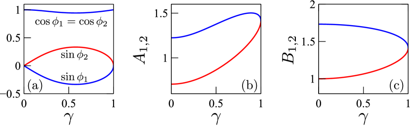
Figure 2: (a): Dependencies $\cos\phi_{1,2}$ and $\sin\phi_{1,2}$ for $\phi_{1,2}$ in Eq. (45) for $\Omega=1$ and changing $\gamma$. (b)-(c) Parameters $A$ and $B$ of bright solitons (51) plotted as functions of $\gamma$ for fixed $\Omega=1$ and $\mu=-2$. In all panels, blue and red curves correspond to symmetric and antisymmetric exact bright solitons, respectively [i.e., to upper and lower signs in Eqs. (44)–(46) and (50)–(51)]. Note that $\cos\phi_{1}=\cos\phi_{2}$, and the corresponding blue and red curve coincide in (a).

4.2 Broken linear ${\cal PT}$ symmetry

For broken linear ${\cal PT}$ symmetry ($\gamma\geq\Omega$), we assume that $\sin\delta=-{\Omega}/{\gamma}$, i.e.,

$$\delta=\delta_{1}=-\arcsin(\Omega/\gamma)\quad\mbox{or}\quad\delta=\delta_{2}=\pi+\arcsin(\Omega/\gamma).$$ (47)

The solution $U\neq 0$ and $V\equiv 0$ is valid if $\phi=0$, $\alpha=\pi/4$ and $U$ solves the NLS equation with linear dissipation ($\delta=\delta_{1}$) or gain ($\delta=\delta_{2}$)

$$iU_{t}=-U_{xx}+i\Omega\cot(\delta)U+2g|U|^{2}U.$$ (48)

The original fields are recovered as

$$u=-i\sqrt{2}\sin(\delta/2)U,\quad v=\sqrt{2}\cos(\delta/2)U.$$ (49)

For $\delta=\delta_{1}$ or $\delta=\delta_{2}$ the total number of particles $N(t)$ decays to zero or grows, respectively. Note that the decaying solution does not violate inequality (31) since the substitution (49) implies identically zero quasi-power (29): $Q(t)=Q(0)=0$. Additionally we note that solution (49) is asymmetric, i.e., the field amplitudes $u$ and $v$ are not equal: $|u/v|=|\tan(\delta/2)|$.

In the particular case of the exceptional point (EP) of the underlying linear ${\cal PT}$-symmetric system, $\Omega=\gamma$, Eq. (48) becomes the integrable conservative NLS equation. Thus the decaying and growing solutions bifurcate from the conservative solution at the EP $\Omega=\gamma$, with $\gamma/\Omega\geq 1$ being the bifurcation parameter.

5 Bright solitons and their dynamics

As we have shown in Sec. 4.1, the introduced Hamiltonian ${\cal PT}$-symmetric system contains as a particular case the standard NLS equation and therefore admits various exact solutions. In this section, we explore an important class of solutions in the form of bright solitons, which can be found for the self-focusing nonlinearity in the NLS equation (46). We therefore assume $g=-1$. Additionally, in this section we set $\Omega=1$. Then, using the results of Sec. 4.1, we readily find two families of bright solitons of system (21):

$$u_{1,2}(x,t)=e^{-i\delta_{1,2}/2}A_{1,2}\mathrm{sech}(B_{1,2}x)e^{-i\mu t},\quad v_{1,2}(x,t)=e^{i\delta_{1,2}}u_{1,2},$$ (50)

where

$$\eqalign{A_{1,2}=\frac{\sqrt{2}}{2}(3\gamma^{2}+1)^{1/4}\sqrt{-\mu\pm\sqrt{1-\gamma^{2}}},\quad B_{1,2}=\sqrt{-\mu\pm\sqrt{1-\gamma^{2}}}.}$$ (51)

Subscripts $1$ and $2$ correspond to upper and lower signs in Eqs. (44)–(46). In what follows, we call the two identified families symmetric (with subscript $1$) and antisymmetric (with subscript $2$), because in the limit $\gamma=0$ the two components are identical for the symmetric solitons ($u_{1}=v_{1}$), but are opposite for antisymmetric solitons ($u_{2}=-v_{2}$).

In Eqs. (50)–(51), $\mu$ is the real parameter which characterizes the temporal frequency of the solution (i.e., the BEC’s chemical potential). From Eqs. (51) it follows that the symmetric solitons exist for $\mu<\sqrt{1-\gamma^{2}}$, and the antisymmetric solitons require $\mu<-\sqrt{1-\gamma^{2}}$. As it is typical for ${\cal PT}$-symmetric systems, the solutions constitute a continuous family: if the parameter $\gamma$ is fixed, one can construct a continuous set of solutions by changing the “internal” parameter $\mu$. Notice however, that for $\gamma$ in the interval $(0,1)$ the families of symmetric and antisymmetric solitons do not coexist, because, as readily follows from Eq. (45), symmetric solitons require $\phi<0$, and antisymmetric solitons exist for $\phi>0$. For fixed $\mu$, branches of symmetric and antisymmetric solitons coalesce at $\gamma=1$ as one can observe in Fig. 2.

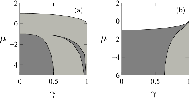
Figure 3: Stability domains for bright symmetric (a) and antisymmetric (b) solitons. White domains correspond to $(\mu,\gamma)$, where the solitons do not exist. Dark gray domains correspond to regions where the solitons exist and stable; light gray domains correspond to unstable solitons.

In order to check the linear stability of solitons, we used the substitution

$$\eqalign{u(x,t)=[e^{-i\delta/2}A\,\mathrm{sech}(Bx)+w(x)e^{\lambda t}+z^{*}(x)e^{\lambda^{*}t}]e^{-i\mu t},\\ v(x,t)=[e^{i\delta/2}A\,\mathrm{sech}(Bx)+W(x)e^{\lambda t}+Z^{*}(x)e^{\lambda^{*}t}]e^{-i\mu t}}$$ (52)

and linearized system (21) with respect to perturbations $(w,z,W,Z)$. [In (52) we omitted subscripts $1$ and $2$ because the linear stability substitution has the same form for symmetric and antisymmetric solitons.] The growth rates of eventual instabilities, given by $\textrm{Re}\,\lambda$, were computed numerically from eigenvalues $\lambda$ of a large sparse matrix which was obtained after approximation of second spatial derivatives using the second finite difference. The outcomes of our stability study are summarized in Fig. 3 which shows that solitons of either type are stable if wide parameter ranges.

Although the reported solitons are exact solutions, the system apparently is not integrable. This raises the question about solitons’ interactions. In order to address this issue, we prepare the initial condition for system (21) in the form of a superposition of two separated solitons (50) which are launched towards each other:

$$u(x,0)=u_{j_{+}}(x-l,0)e^{-icx}+u_{j_{-}}(x+l,0)e^{+icx},$$ (53)

$$v(x,0)=v_{j_{+}}(x-l,0)e^{-icx}+v_{j_{-}}(x+l,0)e^{+icx},$$ (54)

where constants $l\gg 1$ and $c>0$ determine the initial separation between the solitons and initial solitons’ velocity, respectively. Subscripts $j_{+}$ and $j_{-}$ can acquire values $1$ or $2$, depending on the type of the soliton (symmetric or antisymmetric). Both solitons correspond to the same value of the gain-and-loss coefficient $\gamma$ [which is the parameter of the system (21)], but, generically speaking, have different chemical potentials $\mu_{+}$ and $\mu_{-}$ [because the chemical potential does not enter system (21) but represents an internal parameter of each soliton]. Once $\gamma$, $j_{\pm}$, and $\mu_{\pm}$ are chosen, the initial amplitudes and width of the solitons are computed from Eqs. (51). Then the dynamics of system (21) is simulated numerically. Quite surprisingly, in our simulations we observe that the system behaves as nearly integrable, and solitons interact elastically, similarly to the solitons in the integrable NLS equation. In Fig 4(a) we show the collision of two identical antisymmetric in-phase solitons, which pass through each other without any visible distortion. Two out-of phase solitons in Fig. 4(b) elastically repel each other and recover their original shapes. Moreover, in spite of the gain and losses, we also observed elastic interactions of (stable) solitons with considerably different amplitudes, as illustrated in Fig. 4(c). Similar results were also obtained for collisions of symmetric solitons, when their parameters are chosen from the stability domain.

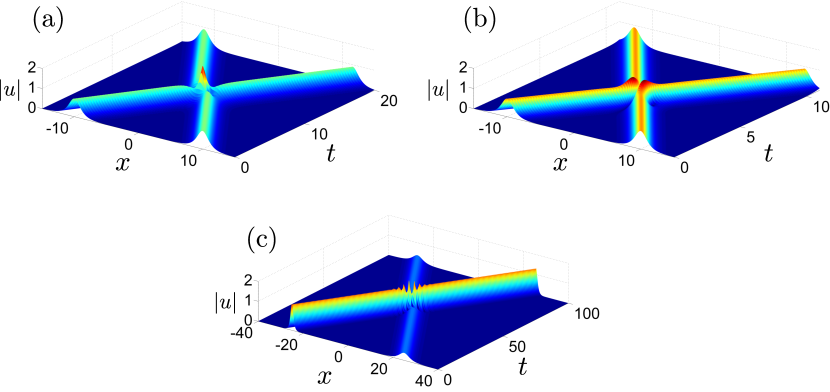
Figure 4: Interactions of stable antisymmetric solitons. (a) Two identical in-phase solitons with $\mu=-2.5$ and $\gamma=0.2$; (b) Two identical out-of-phase solitons with $\mu=-2.5$ and $\gamma=0.2$; (c) Two solitons with $\gamma=0.3$ and different amplitudes: the large-amplitude soliton has $\mu=-4$, and the small-amplitude soliton has $\mu=-0.5$. All panels show the amplitude of field in the first component, i.e., $|u|$; the behavior of the second component $|v|$ is almost identical to $|u|$.

Finally, we explored numerically the dynamics of unstable solitons. To this end, we numerically integrated system (21) with initial conditions in the form (50)–(51) with $t=0$ (small-amplitude random distortions have been introduced in the initial conditions in order to boost the development of an eventual dynamical instability). Three different dynamical scenarios observed for different $\gamma$ and $\mu$ are presented in Fig. 5. The first observed scenario (which was found the most typical for antisymmetric solitons) consists in the infinite growth of the $u$-component (the one that is subjected to the linear gain $i\gamma$) as shown in Fig. 5(a). Because of the fast growth of the amplitude in the first component (i.e., $u$), the numerical process eventually diverges, and the computation terminates; the amplitude of the second component $v$ remains moderated and does not grow (at least until the moment when the numerical process diverges). For symmetric solitons, we recorded two different scenarios: for relatively small gain-and-loss $\gamma$ the instability manifests itself in the emergence of a long-living oscillating (breather-like) mode [Fig. 5(b)], which is another pattern typical to integrable model. For large gain-and-loss $\gamma$ the initially quiescent soliton breaks into a pair of pulses which propagate with different velocities [Fig. 5 (c)]. For dynamics in Fig. 5(b) and (c), behaviors of $u$ and $v$ components are almost identical.

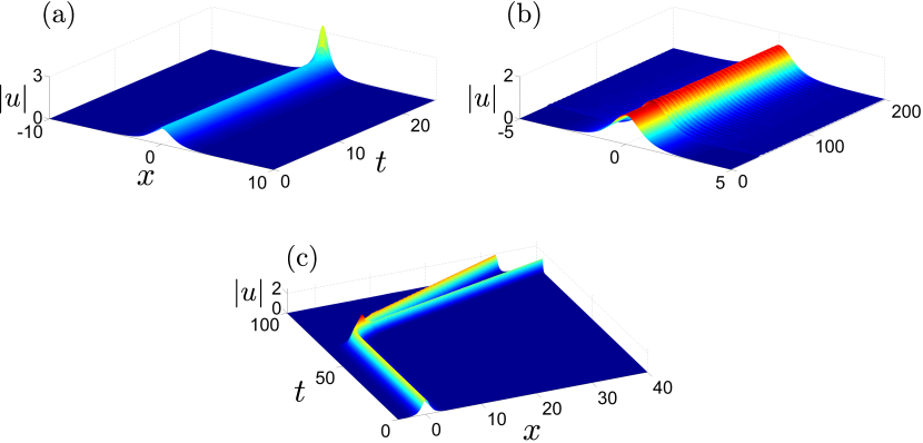
Figure 5: Different behaviours of unstable solitons. (a) Antisymmetric soliton with $\gamma=0.8$ and $\mu=-2$ exhibits the unbounded growth of $|u|$. (b) Symmetric soliton with $\gamma=0.6$ and $\mu=-2$ evolves into a long-living oscillating state. (c) Symmetric soliton with $\gamma=0.95$ and $\mu=-2$ breaks into a pair of spontaneously moving and long-living solitons. All panels show the amplitude of the field in the first component, i.e., $|u|$; the behavior of the second component $v$ is explained in the text.

6 Discussion and Conclusion

In this paper, we proposed and investigated a nonlinear ${\cal PT}$-symmetric coupler which have several remarkable properties. First, it admits Hamiltonian and Lagrangian formulations, which is not a typical property of nonlinear ${\cal PT}$-symmetric systems in general. Second, it has (at least) three conservation laws which can be derived from Noether’s theorem. In the conservative limit, the system becomes bi-Hamiltonian, i.e., admits two different Hamiltonian representations simultaneously. Additionally, the introduced ${\cal PT}$-symmetric coupler supports a variety of exact solutions which can take form of bright and dark solitons or more complex patterns. Moreover, it was demonstrated numerically that some of the exact solutions are dynamically stable and undergo elastic collisions, similar to collisions of solitons of the integrable NLS equation. We have also outlined the physical relevance of the introduced model in the context of Bose-Einstein condensates in nonlinear lattices.

While the main goal of this paper was to introduce a dispersive Hamiltonian ${\cal PT}$-symmetric system, the proposed model admits several generalizations which are worth future study. The first evident generalization of the Hamiltonian (3) suggests to consider the case of two different nonlinear coefficients $g_{1}$ and $g_{2}$, i.e.,

$$H=\int_{-\infty}^{\infty}\left[u_{x}^{*}v_{x}+u_{x}v_{x}^{*}+i\gamma(uv^{*}-u^{*}v)+\Omega(|u|^{2}+|v|^{2})\right.$$

$$\left.\hskip 56.9055pt+(g_{1}|u|^{2}+g_{2}|v|^{2})(e^{i\phi}u^{*}v+e^{-i\phi}uv^{*})\right]dx.$$ (55)

Then the Hamiltonian equations (19) lead to a generalized version of system (21):

$$\eqalign{iu_{t}=-u_{xx}+i\gamma u+\Omega v+g_{1}e^{-i\phi}|u|^{2}u+2g_{2}e^{-i\phi}|v|^{2}u+g_{2}e^{i\phi}u^{*}v^{2},\\ iv_{t}=-v_{xx}-i\gamma v+\Omega u+g_{2}e^{i\phi}|v|^{2}v+2g_{1}e^{i\phi}|u|^{2}v+g_{1}e^{-i\phi}u^{2}v^{*}.}$$ (56)

For $g_{1}\neq g_{2}$ this nonlinear system is not ${\cal PT}$ symmetric (in the sense discussed in Sec. 3). Interestingly enough, this model admits a stationary solitonic solution. Indeed, under the assumptions

$$u=i\cot^{1/2}(\delta/2)U,\quad v=\tan^{1/2}(\delta/2)U,$$ (57)

$$\gamma=\Omega\,\textrm{cosec}\,\delta,\quad g_{2}=-g_{1}\cot^{2}\delta,$$ (58)

where $\delta\in(0,\pi)$ is a free parameter, system (56) reduces to a scalar NLS equation with linear gain or loss (depending on value of $\delta$) and purely imaginary nonlinearity [compare with (48)]:

$$iU_{t}=-U_{xx}+i\Omega\cot(\delta)U+2ig_{1}\cot(\delta/2)\sin\phi|U|^{2}U.$$ (59)

This equation has a well-known stationary solution in the form of the Pereira-Stenflo soliton [29]

$$U=Ae^{-iB^{2}t}\textrm{sech}^{1+i\sqrt{2}}(Bx),$$ (60)

where

$$A^{2}=-\frac{3\Omega\cos\delta}{8g_{1}\sin\phi(1+\cos\delta)},\quad B^{2}=\frac{\Omega\cot(\delta)}{2\sqrt{2}}.$$ (61)

The existence of this stationary solution is remarkable in view of the fact that the coupler operates in the domain of broken ${\cal PT}$ symmetry, i.e., $|\gamma/\Omega|\geq 1$ [as readily follows from the first of equations (58)].

Regarding further generalizations of the introduced models, we notice that while herein we have considered a spatially one-dimensional dispersive system, the Hamiltonian structure is expected to survive in the case of multiple dimensions as well, i.e., for $x\in\mathbb{R}^{D}$, $D\geq 2$. Another potential generalization is related to the possibility to address nonlinear multi-component systems with three (or more) coupled waveguides. Some of such dispersive systems should also admit Hamiltonian structure.

References

References

-
[1]
Bender C M and Boettcher S 1998
Real spectra in mon-Hermitian Hamiltonians having symmetry,
Phys. Rev. Lett. 80, 5243–5246 (1998).
Bender C M 2007 Making sense of non-Hermitian Hamiltonians Rep. Prog. Phys. 70 947. -
[2]
Mostafazadeh A 2003 Exact PT-symmetry is equivalent to Hermiticity
J. Phys. A: Math. Gen. 36 7081–7091
Mostafazadeh A 2009 Non-Hermitian Hamiltonians with a real spectrum and and their physical applications Pramana J. Phys. 73 269–277. - [3] Konotop V V, Yang J and Zezyulin D A 2016 Nonlinear waves in -symmetric systems Rev. Mod. Phys. 88 35002.
- [4] El-Ganainy R, Makris K G, Christodoulides D N, and Musslimani Z H 2007 Theory of coupled optical -symmetric structures Opt. Lett. 32 2632.
- [5] Rüter C E, Makris K G, El-Ganainy R, Christodoulides D N, Segev M, and Kip D 2010 Observation of parity-time symmetry in optics Nature Phys. 6 192.
- [6] Bender C M, Gianfreda M, Özdemir Ş K, Peng B, and Yang L 2013 Twofold transition in PT-symmetric coupled oscillators Phys. Rev. A 88 062111.
- [7] Ramezani H, Kottos T, El-Ganainy R, and Christodoulides D N Unidirectional nonlinear PT-symmetric optical structures 2010 Phys. Rev. A 82 043803.
- [8] Barashenkov I V and Gianfreda M 2014 An exactly solvable -symmetric dimer from a Hamiltonian system of nonlinear oscillators with gain and loss J. Phys. A: Math. Theor. 47 282001.
- [9] Barashenkov I V 2014 Hamiltonian formulation of the standard PT-symmetric nonlinear Schrödinger dimer Phys. Rev. A. 90 045802.
- [10] Jørgensen M F and Christiansen P L 1993 Hamiltonian structure for a modified discrete self- trapping dimer Chaos, Solitons and Fractals 4 217–225.
- [11] Jørgensen M F, Christiansen P L, and Abou-Hayt I 1993 On a modified discrete self-trapping dimer Physica D 68 180–184.
- [12] Barashenkov I V, Pelinovsky D E, and Dubard P 2015 Dimer with gain and loss: Integrability and -symmetry restoration J. Phys. A: Math. Theor. 48 325201.
-
[13]
Chernyavsky A and Pelinovsky D E 2016 Breathers in Hamiltonian -Symmetric Chains of
Coupled Pendula under a Resonant Periodic Force Symmetry 8 59
Chernyavsky A and Pelinovsky D E 2016 Long-time stability of breathers in Hamiltonian -symmetric lattices J. Phys. A: Math. Theor. 49 475201. -
[14]
Politi A, Oppo G L, and Badii R 1986
Coexistence of conservative and dissipative behavior in reversible dynamical systems Phys. Rev. A 33 4055
Altmann E G, Cristadoro G, and Pazo D 2006 Nontwist non-Hamiltonian systems Phys. Rev. E 73 056201
Sprott J C 2014 A dynamical system with a strange attractor and invariant tori Phys. Lett. A 378 1361. - [15] Morsch O and Oberthaler M 2006 Dynamics of Bose-Einstein condensates in optical lattices Rev. Mod. Phys. 78 179.
- [16] Yamazaki R, Taie S, Sugawa S and Takahashi Y 2010 Submicron Spatial Modulation of an Interatomic Interaction in a Bose-Einstein Condensate Phys. Rev. Lett. 105 050405.
-
[17]
da Luz H L F, Abdullaev F Kh, Gammal A, Salerno M and Tomio L 2010
Matter-wave two-dimensional solitons in crossed linear and nonlinear optical lattices
Phys. Rev. A 82 043618
Qi Ran and Zhai Hui 2011 Bound States and Scattering Resonances Induced by Spatially Modulated Interactions Phys. Rev. Lett 106 163201
Yulin A V, Bludov Yu V, Konotop V V, Kuzmiak V and Salerno M 2011 Superfluidity of Bose-Einstein condensates in toroidal traps with nonlinear lattices Phys. Rev. A 84 063638
Kartashov, Y V, Malomed B A and Torner L 2011 Solitons in nonlinear lattices Rev. Mod. Phys. 83 247
Salasnich L and Malomed B A 2012 Quasi-one-dimensional Bose-Einstein condensates in nonlinear lattices J. Phys. B: At. Mol. Opt. Phys. 45 055302
Lebedev M E, Alfimov G L and Malomed B A 2016 Stable dipole solitons and soliton complexes in the nonlinear Schrödinger equation with periodically modulated nonlinearity Chaos 26 073110. -
[18]
Wasak T, Konotop V V and Trippenbach M 2013 Atom laser based on four-wave mixing with Bose-Einstein condensates in nonlinear lattices Phys. Rev. A 88 063626
Wasak T, Konotop V V and Trippenbach M 2014 Four-wave mixing with Bose-Einstein condensates in nonlinear lattices EPL 105 64002. -
[19]
Hilligsøe K M and Mølmer K 2005 Phase-matched four wave mixing and quantum beam splitting of matter waves in a periodic potential Phys. Rev. A 71 041602(R)
Pertot D, Gadway B and Schneble D 2010 Collinear Four-Wave Mixing of Two-Component Matter Waves Phys. Rev. Lett. 104 200402
Campbell G K, Mun J, Boyd M, Streed E W, Ketterle W, and Pritchard D E 2006 Parametric Amplification of Scattered Atom Pairs Phys. Rev. Lett. 96 020406. - [20] Konotop V V and Salerno M 2002 Modulational instability in Bose-Einstein condensates in optical lattices Phys. Rev. A 65 021602(R).
- [21] Gerdjikov V S 2017 private communication.
- [22] Barashenkov I V 2017 private communication.
- [23] Ablowitz M J and Clarkson P A 1991 Solitons, Nonlinear Evolution Equations and Inverse Scattering (Cambridge University Press)
- [24] Wasak T, Szańkowski P, Konotop V V and Trippenbach M 2015 Four-wave mixing in a parity-time ()-symmetric coupler Opt. Lett. 40 5291.
- [25] Sulem C and Sulem P-L 1999 The Nonlinear Schrödinger Equation (Springer, New York)
- [26] Driben R and Malomed B A 2011 Stability of solitons in parity-time-symmetric couplers Opt. Lett. 36 4323.
- [27] Peregrine D H 1983 Water waves, nonlinear Schrödinger equations and their solutions J. Austral. Math. Soc. B, Appl. Math. 25 16–43.
- [28] Akhmediev N N, Eleonskii V M, Kulagin N E 1987 Exact first-order solutions of the nonlinear Schrödinger equation Theor. Math. Phys. 72 809–818 [Teoreticheskaya i Matematicheskaya Fizika 72 183–196].
-
[29]
Hocking L M and Stewartson K 1972 On the nonlinear response of a marginally unstable plane parallel flow to a 2-dimensional disturbance Proc. R. Soc. A 326 289–313 (1972)
Pereira N R and Stenflo L 1977 Nonlinear Schrödinger equation including growth and damping Phys. of Fluids 20 1733–1734.