Classification of Quench Dynamical Behaviours in Spinor Condensates

Abstract

Thermalization of isolated quantum systems is a long-standing fundamental problem where different mechanisms are proposed over time. We contribute to this discussion by classifying the diverse quench dynamical behaviours of spin-1 Bose-Einstein condensates, which includes well-defined quantum collapse and revivals, thermalization, and certain special cases. These special cases are either nonthermal equilibration with no revival but a collapse even though the system has finite degrees of freedom or no equilibration with no collapse and revival. Given that some integrable systems are already shown to demonstrate the weak form of eigenstate thermalization hypothesis (ETH), we determine the regions where ETH holds and fails in this integrable isolated quantum system. The reason behind both thermalizing and nonthermalizing behaviours in the same model under different initial conditions is linked to the discussion of ‘rare’ nonthermal states existing in the spectrum. We also propose a method to predict the collapse and revival time scales and find how they scale with the number of particles in the condensate. We use a sudden quench to drive the system to non-equilibrium and hence the theoretical predictions given in this paper can be probed in experiments.

I Introduction

Understanding if and how isolated quantum systems driven out-of-equilibrium thermalize has practical implications as well as being interesting from a fundamental point of view. Being able to explain the thermalizing dynamics in an isolated system is the key to have quantum thermal baths Fialko and Hallwood (2012); Fialko (2015). Thermalization of quantum systems also sheds light on how the statistical mechanics emerge from unitary dynamics of quantum mechanics Kaufman et al. (2016); Neill et al. (2016). At the opposite side, nonthermalizing quantum systems might be useful to store quantum information in the protected degrees of freedom Nandkishore and Huse (2015); Huse et al. (2013).

Study of thermalization of isolated quantum systems has a long history that starts with the development of quantum mechanics itself von Neumann (2010) and can be understood in the context of Eigenstate Thermalization Hypothesis (ETH) for isolated systems Deutsch (1991); Srednicki (1994); Jensen and Shankar (1985); Rigol et al. (2008); Polkovnikov et al. (2011). In this search to understand quantum thermalization, analogue concepts which are important in the thermalization of classical systems have been drawn such as the integrability of the system Fermi et al. (1955); Rigol et al. (2007). In this paper, we study dynamics of the spin-$1$ spinor Bose-Einstein condensate (BEC) system under single-mode approximation (SMA), which is known to be a quantum-integrable model Tabor (1989) based on its mean-field calculations Romano and de Passos (2004); Zhang et al. (2005). The consensus is that quantum-integrable systems do not thermalize according to statistical ensembles, but they obey the predictions of generalized Gibbs ensemble which takes into account the conservation properties in the system Hamiltonian Rigol et al. (2007) in the aim of maximizing the entropy of the system under study Jaynes (1957). However, it has also been shown that the non-integrability does not always point to thermalization Gogolin et al. (2011); Manmana et al. (2007); Kollath et al. (2007); Shiraishi and Mori (2017) and some integrable systems, e.g. Lieb-Liniger model and integrable spin chains, do show thermalization in the form of weak ETH Biroli et al. (2010); Ikeda et al. (2013); Alba (2015). In fact, it seems that what differentiates a quantum integrable system from a non-integrable one in the context of thermalization is not that the system can thermalize or not, but instead having ‘rare’ nonthermal eigenstates in the spectrum that do not disappear in the thermodynamic limit Biroli et al. (2010). Our results of spinor condensate model support this idea of quantum thermalization for a specific region of Hamiltonian parameters, where we observe a spectrum composed of mostly ‘typical’ thermal states with some ‘rare’ nonthermal ones. The exact diagonalization of spin-1 condensate under the SMA for realistic condensate sizes provides us the opportunity to dig into the whole spectrum of eigenstates and determine the regions where ETH is applicable based on the condition in Ref. Rigol et al. (2008). Then we show that these regions in the spectrum are composed of ‘typical’ thermal eigenstates that lead to vanishing fluctuations and shrinking support in the thermodynamic limit Biroli et al. (2010); Ikeda et al. (2013). We apply some other ETH indicators, as well, such as the scaling of eigenstate expectation value differences Kim et al. (2014); Pal and Huse (2010) and the scaling of the maximum divergence from the microcanonical ensemble average Shiraishi and Mori (2017) with the system size. The scaling exponents match with each other and all of them point to the observation that in the thermodynamic limit spinor condensates thermalize for certain initial conditions (but not for all initial conditions), implying the weak form of ETH. Given the fact that ultracold atoms provide a highly controllable and a sufficiently isolated system Polkovnikov et al. (2011), we show that a spin-1 spinor condensate under the SMA could be a testbench to observe the predictions of ETH for certain sudden quench parameters and the transition between thermalization and nonthermalization without a need to add a non-integrable perturbation to an integrable Hamiltonian Yurovsky and Olshanii (2011); Manmana et al. (2007); Canovi et al. (2011). In fact, being able to see this transition without breaking the integrability of the model hints at that the thermalization is not directly tied to non-integrability Manmana et al. (2007). Instead, it might be more relevant to consider the localization properties of the spectrum to observe thermalizing behaviour in isolated quantum systems Canovi et al. (2011); Pal and Huse (2010). Therefore, by invoking the analogy between our model and the single quantum-particle hopping model and hence calculating the participation ratios Evers and Mirlin (2008) that is a widely-used tool for Anderson models Anderson (1958), we show that the most localized eigenstates in the spectrum (excluding the edges of the spectrum) are also the ‘rare’ nonthermal eigenstates that cause nonthermalization behaviour in the system.

Quantum collapse and revivals are well-known phenomena observed in different systems spanning from light-matter interactions in Jaynes-Cummings model Scully and Zubairy (1997) to Bose-Hubbard models in optical lattices Kollath et al. (2007); Will et al. (2010) and the matter wave field of a BEC Greiner et al. (2002). This kind of behaviour is also expected in discrete and finite systems due to the recurrence theorem Bocchieri and Loinger (1957). The possibility that spin-1 BEC under the SMA might also demonstrate collapse and revivals has been suggested in Ref. Law et al. (1998); Pu et al. (2000) and a detailed analysis of collapses with specific initial Fock states in this model has been given Pu et al. (1999). These full-quantum model studies did not take the Zeeman effects into account, partly because the model without Zeeman effects has rotational symmetry and is analytically solvable via the introduction of angular momentum-like operators in the Fock basis Law et al. (1998). On the other hand, the experiments of the spinor BECs make use of the quadratic Zeeman effect as a control parameter to sweep across the well-established phase transitions Stamper-Kurn and Ueda (2013); Sadler et al. (2006); Zhang and Duan (2013) that spinor BECs have in their mean-field representation Zhang et al. (2003). With the introduction of quadratic Zeeman effect, at the mean-field level the physics is mapped to an analytical pendulum-like model Zhang et al. (2005). Some of the mean-field predictions have been experimentally verified Jiang et al. (2014). However, the mean-field model cannot capture the quantum collapse and revivals of the full-quantum Hamiltonian. In the second part of our paper, we calculate the time scales for quantum collapse and revivals in the spin-$1$ condensate model in the parameter region where they exist and show that under realistic conditions and condensate sizes the system equilibrates around its thermal value, validating the ETH for our model. Finally, we discuss some particular parameter regions where we observe only equilibration but not thermalization without quantum revivals in any time-scale of the evolution. This is somewhat unexpected given the fact that our model is a discrete system with finite degrees of freedom and the initial information tends to recur in long-time scale for finite-size systems.

II Classification of Dynamical Behaviours under Sudden Quench of Spin-1 Spinor Condensate

The interaction Hamiltonian for a spin-$1$ BEC in the second-quantization picture takes the form Stamper-Kurn and Ueda (2013)

$$\hat{H}_{\text{int}}=\frac{1}{2}\int d\mathbf{r}\left(c_{0}^{\prime}:\hat{n}^{2}(\mathbf{r}):+c_{1}^{\prime}:\hat{F}^{2}(\mathbf{r}):\right),$$ (1)

where $::$ denotes the normal ordering. The coefficients in the interaction Hamiltonian depend on the scattering length and the atom mass through

$$c_{0}^{\prime} = \frac{4\pi\hbar^{2}}{M}\frac{a_{0}+2a_{2}}{3},$$

$$c_{1}^{\prime} = \frac{4\pi\hbar^{2}}{M}\frac{a_{2}-a_{0}}{3},$$ (2)

where $a_{0}$ and $a_{2}$ are the scattering lengths corresponding to a total spin $0$ and a total spin $2$ of the colliding atoms. The operators in the interaction Hamiltonian are defined by

$$\hat{n}(\mathbf{r}) = \sum_{m,n=-1}^{1}\hat{\psi}_{m}^{\dagger}(\mathbf{r})I_{mn}\hat{\psi}_{n}(\mathbf{r}),$$

$$\hat{F_{\nu}}(\mathbf{r}) = \sum_{m,n=-1}^{1}\hat{\psi}_{m}^{\dagger}(\mathbf{r})(F_{\nu})_{mn}\hat{\psi}_{n}(\mathbf{r}),$$ (3)

where $\hat{\psi}_{m_{F}}$ $\left(\hat{\psi}_{m_{F}}^{\dagger}\right)$ is the Bose field operator for the Zeeman state $m_{F}$. $I_{mn}$ and $(F_{\nu})_{mn}$ are the identity and spin-1 matrices, respectively and $\nu=x,y,z$ in the angular momentum operator $\hat{F_{\nu}}$. Also note that $\hat{F}^{2}(\mathbf{r})=\hat{F}^{2}_{x}(\mathbf{r})+\hat{F}^{2}_{y}(\mathbf{r})+\hat{F}^{2}_{z}(\mathbf{r})$ in Eq. (1) and the identity matrix $I_{mn}$ results in the density operator $\hat{n}(\mathbf{r})$ for the condensate. For sodium or rubidium alkali atoms, we have $|c_{0}^{\prime}|\gg|c_{1}^{\prime}|$, so the symmetric part of the interaction Hamiltonian dominates over the non-symmetric part. This observation leads to the so-called single mode approximation (SMA), where we assume that the condensate wave functions for each spin component $\phi_{m=-1,0,1}(\mathbf{r})$ are described by the same spatial wave function $\phi(\mathbf{r})$ as in $\hat{\psi}_{m}\sim\hat{a}_{m}\phi(\mathbf{r}),\hskip 8.53581ptm=0,\pm 1$ Stamper-Kurn and Ueda (2013); Law et al. (1998); Zhang et al. (2003); Yi et al. (2002). Then the spatial wave function $\phi(\mathbf{r})$ satisfies the Gross-Pitaevskii equation which gives the spatial profile of our spin-1 Bose-Einstein condensate. With the normalization condition $\int d\mathbf{r}|\phi(\mathbf{r})|^{2}=1$, the interaction Hamiltonian reduces to rotationally invariant $H_{\text{int}}=c_{1}\hat{L}^{2}/2N$, where $\hat{L}$ is the spin-1 angular momentum operator, $c_{1}=c_{1}^{\prime}N\int d\mathbf{r}|\phi(\mathbf{r})|^{4}$ and $N$ is the total atom number, which has well-known analytical solutions Law et al. (1998). In the experiment, an additional magnetic Zeeman field is added to the system, which results in a competition between different terms in the Hamiltonian and drives phase transitions Zhang and Duan (2013). The linear Zeeman term proportional to $\hat{L}_{z}=\hat{n}_{1}-\hat{n}_{-1}$ commutes with the other terms in the Hamiltonian, and its effect is to conserve the magnetization. It has no influence on spin dynamics and therefore can be dropped Zhang and Duan (2013). Adding the quadratic Zeeman term, the Hamiltonian reduces to

$$H_{\text{int}} = c_{1}\frac{\hat{L}^{2}}{N}-q\hat{a}_{0}^{\dagger}\hat{a}_{0},$$ (4)

$$= \frac{c_{1}}{N}(\hat{a}_{1}^{\dagger}\hat{a}_{1}^{\dagger}\hat{a}_{1}\hat{a}_{1}+\hat{a}_{-1}^{\dagger}\hat{a}_{-1}^{\dagger}\hat{a}_{-1}\hat{a}_{-1}-2\hat{a}_{1}^{\dagger}\hat{a}_{-1}^{\dagger}\hat{a}_{1}\hat{a}_{-1}$$

$$+ 2\hat{a}_{1}^{\dagger}\hat{a}_{0}^{\dagger}\hat{a}_{0}\hat{a}_{1}+2\hat{a}_{-1}^{\dagger}\hat{a}_{0}^{\dagger}\hat{a}_{0}\hat{a}_{-1}+2\hat{a}_{0}^{\dagger}\hat{a}_{0}^{\dagger}\hat{a}_{1}\hat{a}_{-1}$$

$$+ 2\hat{a}_{1}^{\dagger}\hat{a}_{-1}^{\dagger}\hat{a}_{0}\hat{a}_{0})-q\hat{a}_{0}^{\dagger}\hat{a}_{0}.$$

Spin-1 BEC Hamiltonian with the quadratic Zeeman term gives rise to different phases observed at the ground state due to the competition between quadratic Zeeman effect and spin-mixing interaction Jiang et al. (2014). An adiabatic passage from one phase to another can create highly entangled states from product states as proposed in Ref. Zhang and Duan (2013) and quite recently implemented in Ref. Luo et al. (2017). Fig. 1 shows the ground state quantum phase transitions by observing the order parameter $\Braket{N_{0}}$, the number of particles in Zeeman sublevel $\Ket{m=0}$, by varying the quadratic Zeeman coefficient $q$.

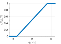
(a)

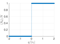
(b)

Figure 1: The ground state phase transitions for (a) ferromagnetic and (b) anti-ferromagnetic interactions for $N=10^{4}$ particles in the condensate and zero total magnetization.

In the rest of the paper, we study the dynamics of the system under a sudden quench, i.e., we start from the ground state of the initial Hamiltonian $H_{i}$, which is $H_{\text{int}}$ (Eq. (4)) with an initial quadratic Zeeman term $q_{i}$, and abruptly quench the Zeeman field to a final value $q_{f}$ with the final Hamiltonian denoted as $H_{f}$. The dynamics and thermalization behaviour of the system are then investigated. Both the sudden quench and the measurement of $\Braket{N_{0}}$, which is used as the main observable in our study, can be readily performed in experiment Jiang et al. (2014); Liu et al. (2009); Hoang et al. (2016); Anquez et al. (2016).

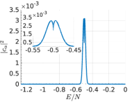
(a)

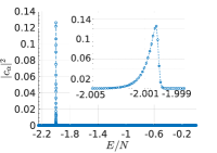
(b)

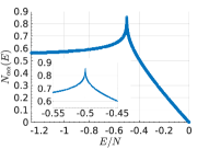
(c)

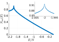
(d)

Figure 2: Eigenstate occupation numbers (EONs) $|c_{\alpha}|^{2}$ for a ferromagnetic quench at (a) $q_{i}=-3$ to $q_{f}=0.5$ and (b) $q_{i}=4.1$ to $q_{f}=2$ (focused on non-zero sections of the eigenspectrum in the insets) and their corresponding eigenstate expectation values (EEVs) (focused on the nonlinear kink region in the insets) $N_{\alpha\alpha}$ at (c) and (d), respectively for a particle number of $10^{4}$ with respect to the energy density $E/N$.

We now show how a dynamical phase transition (DPT) might be arising for spinor condensates via the sudden quench based on an alternative definition of DPTs that takes the time-average of dynamical response as the order parameter Zunkovic et al. (2016); Zhang et al. (2017). In our study, we start with the ground state, $\Ket{\psi(0)}$ of the initial Hamiltonian $H_{i}$ with $q=q_{i}$. After a sudden quench of the Zeeman coefficient $q$ to the value $q_{f}$, the initial state can be expressed as

$$\Ket{\psi(0)}=\sum_{\alpha}c_{\alpha}\Ket{\psi_{\alpha}},$$ (5)

where $\Ket{\psi_{\alpha}}$ are the eigenstates of the final Hamiltonian $H_{f}$. The number of atoms in the Zeeman sublevel $\Ket{m=0}$ can be written as

$$\Braket{N_{0}(t)} = \Bra{\psi(t)}N_{0}\Ket{\psi(t)},$$ (6)

$$= \sum_{\alpha,\beta}c_{\alpha}^{\ast}c_{\beta}e^{-i(E_{\alpha}-E_{\beta})t}N_{0,\alpha\beta},$$

where $N_{0,\alpha\beta}=\Bra{\psi_{\alpha}}N_{0}\Ket{\psi_{\beta}}$ and $E_{\alpha}$ are the energy of the eigenstate $\Ket{\psi_{\alpha}}$ under the final Hamiltonian $H_{f}$. The long-time average of $\Braket{N_{0}(t)}$ then should follow the diagonal ensemble prediction Rigol et al. (2008); Rigol (2009); Polkovnikov et al. (2011),

$$\overline{\Braket{N_{0}(t)}}_{t\rightarrow\infty}=\sum_{\alpha}|c_{\alpha}|^{2}N_{0,\alpha\alpha},$$ (7)

if the equilibration happens or when the phase coherence diminishes. In order to visualize this quantity, in Figs. 2a and 2b we plot the eigenstate occupation numbers (EONs) $|c_{\alpha}|^{2}$ for certain sudden quench parameters (seen in the caption). EONs represent windows in the eigenspectrum where we are allowed to peak into when we make a measurement. Figs. 2c and 2d are plots of the corresponding eigenstate expectation values (EEVs) $N_{0,\alpha\alpha}$. What we expect to see in the long-time average of a sudden quench experiment is the summation of EEVs weighted with EONs as shown by Eq. (7).

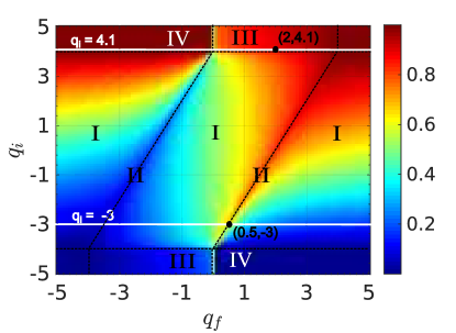
Figure 3: (Color online) The sudden quench map for the ferromagnetic case with $q_{f}$ and $q_{i}$ on the x and y axes, respectively for $5\times 10^{3}$ particles. Color labels $\overline{\Braket{N_{0}(t)}}$ in the long time limit.

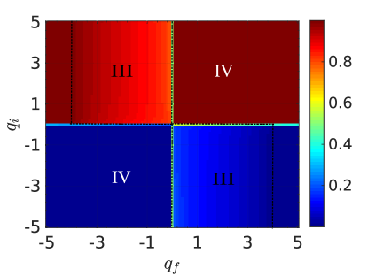
Figure 4: (Color online) The sudden quench map for the anti-ferromagnetic case with $q_{f}$ and $q_{i}$ on the x and y axes, respectively for $5\times 10^{3}$ particles. Color labels $\overline{\Braket{N_{0}(t)}}$ in the long time limit.

Region	Boundaries	Dynamic Behaviour
I	$|q_{i}|<4$, all $q_{f}$ except traces	ETH valid, well-defined collapse and revivals
II	$|q_{i}|<4$, traces of $q_{f}$	nonthermal equilibration, collapse, no revival
III	$q_{i}>4$ $\&$ $0<q_{f}<4$ or $q_{i}<-4$ $\&$ $-4<q_{f}<0$	no equilibration, no collapse or revival
IV	the rest of the map	no non-equilibrium evolution

Table 1: The regions of the sudden quench map for the ferromagnetic case.

Each point on sudden quench maps (Figs. 3 and 4) corresponds to the prediction of diagonal ensemble (equilibration value if it happens, or the time-average of the dynamic response of the system) when a sudden quench is applied to the ground state from an initial Hamiltonian with $q_{i}$ to a final Hamiltonian with $q_{f}$. Note that there are different regions on both maps and the ferromagnetic sudden quench map is more diverse than the anti-ferromagnetic one when the ground state is chosen as the initial state of the non-equilibrium process. Due to the symmetry embedded in the Hamiltonian for both interactions, one can obtain point symmetric version of Fig. 3 (reflection with respect to the origin of the plot) with anti-ferromagnetic interaction when the initial state is set as the most-excited state of the Hamiltonian.

These maps capture the ground state phase transition points of both FM ($q=\pm 4$) and AFM ($q=0$) cases. In Fig. 4, the upper half ($q_{i}>0$) of the map plane reveals two different regions with transition points at $q_{f}=-4$ and $q_{f}=0$. Similarly for the lower half ($q_{i}<0$), we observe two regions with the transition points at $q_{f}=0$ and $q_{f}=4$. In Fig. 3, for $|q_{i}|>4$ we see a similar behaviour to Fig. 4 with transition points either at $q_{f}=0$ and $q_{f}=4$ (for $q_{i}>4$) or at $q_{f}=-4$ and $q_{f}=0$ (for $q_{i}<-4$). In between $|q_{i}|<4$, the two transition points gradually shift as $q_{i}$ increases. In later sections, we are going to show that the sudden quench maps also show us when we do and do not expect a thermal behaviour in our system, similar to the non-equilibrium phase diagram given for Bose-Hubbard model in Ref. Kollath et al. (2007). Additionally it will provide us a way to predict types of the dynamical behaviour in different time scales. To give an idea of the regions on the maps, we summarized them in Table 1. Although the non-equilibrium behaviour of these regions will be explained in detail in the rest of the paper, we shortly list them here. Region I is where the system equilibrates around its thermal prediction after a collapse with a well-defined time-scale. It is also a region where we observe clear quantum revivals due to finite-size effects. Region II demonstrates nonthermal equilibration after a collapse, but no clear collective-revival is observed for these points on the map. We do not see equilibration, collapse or revival for the region III, instead we observe an oscillatory behaviour around the system’s PDE value due to the interference of a small number of modes of the system. Finally in region IV, the initial state turns out to be already in equilibrium with the quench Hamiltonian, giving us practically a constant behaviour for all times.

III Eigenstate Thermalization Hypothesis in Spin-1 BEC

When a system that is driven out-of-equilibrium equilibrates around a thermal value predicted by a statistical ensemble, the process is called thermalization. For isolated interacting bodies, microcanonical ensemble describes the equilibrium predictions. In this context, ETH is a possible pathway to thermalization and explains the match between the equilibration value predicted by the diagonal ensemble after a quench (Eq. (7)) and the microcanonical thermal value Rigol et al. (2008).

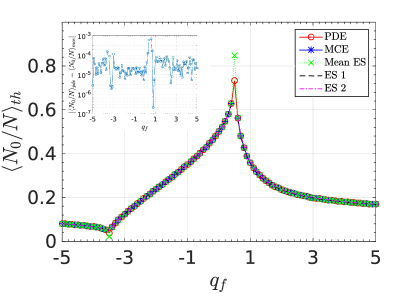
Figure 5: (Color online) The comparison of mean values predicted by diagonal ensemble (PDE), microcanonical ensemble (MCE), the eigenstate corresponding to the mean energy of the system (Mean ES) and arbitrary eigenstates in the microcanonical energy window (ES 1 and ES 2), when the sudden quench is applied from $q_{i}=-3$ to different $q_{f}$ values on the x-axis for ferromagnetic case. Each data point is obtained with a simulation of $10^{4}$ particles. The inset shows the difference between the diagonal and the microcanonical ensemble predictions when it is possible to define a valid energy interval for the microcanonical ensemble.

The microcanonical ensemble is a statistical ensemble with a sufficiently narrow energy interval that describes the equilibrium dynamics of an isolated system Kardar (2007). In order to check the prediction of microcanonical ensemble, we seek to define a narrow energy window around the mean energy of the eigenspectrum. Refs. Rigol et al. (2008); Dunjko and Olshanii ; Rigol (2009) emphasize the approximate linearity of the EEVs in the microcanonical energy window in order to define a finite and narrow energy window which will also ensure the validity of ETH. Based on this idea, they state the following condition (which has been derived for the eigenstate thermalization to happen by Ref. Srednicki (1996))

$$\left(\delta E\right)^{2}|\Braket{N_{0}}^{\prime\prime}(E)/\Braket{N_{0}}(E)|\ll 1,$$ (8)

where $\delta E$ is the energy window, $\Braket{N_{0}}(E)$ is the EEV behaviour of the system $N_{0,\alpha\alpha}$ as a function of the energy and ^′ denotes the differentiation with respect to energy. Another possibility implemented in Ref. Rigol et al. (2008) is to define the window based on a sensitivity analysis where the size of the energy window chosen does not affect the thermal prediction of the microcanonical ensemble (see App. A for a demonstration of this method for our model). We generate the finite and narrow microcanonical energy windows for our model with a combination of these two ways. Figs. 5 and 6 show the regions where the thermal prediction of diagonal ensemble (PDE) matches the prediction of microcanonical ensemble (MCE), mean energy eigenstate (Mean ES) and two arbitrary eigenstates (ES 1 and ES 2) in the microcanonical energy window when it is possible to define one for a sudden quench from $q_{i}=-3$ and $q_{i}=4.1$ to various $q_{f}$ spanning from $-5$ to $5$, respectively. It is important to note that the match happens only when the EON window coincides with the approximately linear or constant parts of the EEV plot. See Fig. 2 for the cases where the match does not happen, so that the system fails to thermalize. Hence, we conclude that the relaxation in the matching cases represents thermalization via ETH, when we disregard the finite-size effects, e.g. a quantum revival, which will be discussed in the next section.

In order to strengthen the argument that we see a nonthermal behaviour only when EON captures the non-linear ‘kink’ behaviour in the EEV spectrum, we look at a couple of ETH indicators. These indicators are also used to determine the form of ETH observed in the system, e.g. weak or strong, if there is thermalization and they require an energy interval over the spectrum. It is possible to define a microcanonical ensemble energy window at the linear region of the spectrum with the methods mentioned above, while such a window is not well-defined for the kink region. Since we want to compare two cases, we define a fixed energy interval around the center of the spectrum.

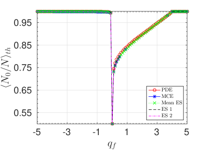
Figure 6: (Color online) The comparison of mean values predicted by diagonal ensemble (PDE), microcanonical ensemble (MCE), the eigenstate corresponding to the mean energy of the system (Mean ES) and arbitrary eigenstates in the microcanonical energy window (ES 1 and ES 2), when the sudden quench is applied from $q_{i}=4.1$ to different $q_{f}$ values on the x-axis for ferromagnetic case. Each data point is obtained with a simulation of $10^{4}$ particles.

The first ETH indicator that we applied is the system size scaling of average EEV differences Pal and Huse (2010); Kim et al. (2014). An EEV difference is defined as

$$r_{n}=|\Bra{\psi_{n+1}}N_{0}\Ket{\psi_{n+1}}-\Bra{\psi_{n}}N_{0}\Ket{\psi_{n}}|,$$ (9)

for random eigenstate $\Ket{\psi_{n}}$ chosen in the energy interval and its adjacent state $\Ket{\psi_{n+1}}$. Regardless of the interval size, when the interval encompasses the linear region as for $q_{f}=3$ in Fig. 7, we obtain the $N^{-1}$ scaling with $R^{2}=1$. Therefore the average of differences between EEVs vanish in the thermodynamic limit $N\rightarrow\infty$. Other indicators are: the ETH noise or fluctuations Biroli et al. (2010); Ikeda et al. (2013)

$$\sigma_{N_{0}} = \left(\frac{\sum_{\psi_{n}\in\delta E}\left[\Bra{\psi_{n}}N_{0}\Ket{\psi_{n}}-\Braket{N_{0}}_{mc,\delta E}\right]^{2}}{N_{\text{int}}}\right)^{1/2},$$ (10)

where the $N_{\text{int}}$ is the number of eigenstates in the chosen interval, $\Braket{N_{0}}_{mc,\delta E}$ is the microcanonical prediction defined in the energy interval of $\delta E$ and $\Ket{\psi_{n}}\in\delta E$ are the eigenstates in the energy interval; the support of the eigenstate distribution in the energy interval Biroli et al. (2010); Ikeda et al. (2013),

$$s_{N_{0}} = \text{max}_{\psi_{n}\in\delta E}\Bra{\psi_{n}}N_{0}\Ket{\psi_{n}}$$ (11)

$$- \text{min}_{\psi_{n}\in\delta E}\Bra{\psi_{n}}N_{0}\Ket{\psi_{n}},$$

and the maximum divergence from the microcanonical ensemble prediction Shiraishi and Mori (2017),

$$r_{\text{max}} = \text{max}_{n}|\Bra{\psi_{n}}N_{0}\Ket{\psi_{n}}-\Braket{N_{0}}_{\text{mc},\delta E}|,$$ (12)

in Fig. 7 across the energy interval chosen. We obtain $N^{-1}$ scaling with $R^{2}=1$ for all these ETH indicators for the aforementioned case. The extracted scaling exponent of the support Eq. (11) clearly indicates in the thermodynamic limit all of the eigenstates in the energy interval contribute the same amount to the expectation value. Furthermore the rest of the ETH indicators, Eqs. (10) and (12), reveals that all of the EEVs in the energy interval converge to the microcanonical energy prediction $\Braket{N_{0}}_{\text{mc},\delta E}$ as $N\rightarrow\infty$. Also note that $N^{-1}$ scaling is not surprising, since the dimension of the Hilbert space is in the order of $N$ for our model.

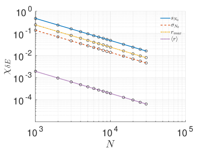
Figure 7: (Color online) The system size scaling of the support $\chi_{\delta E}=s_{N_{0}}$ (solid-blue), the fluctuations (or the ETH noise) $\chi_{\delta E}=\sigma_{N_{0}}$ (dashed-red), the maximum divergence of EEV differences from the MC prediction $\chi_{\delta E}=r_{\text{max}}$ (dashed-dotted orange) and the average EEV difference $\chi_{\delta E}=\langle r_{n}\rangle_{\delta E}$ (dotted purple) for a fixed energy interval when the interval is chosen right at the middle of the spectrum for $q_{f}=3$. All of the scalings show a trend of $N^{-1}$ with $R^{2}=1$ where $R$ is the correlation coefficient.

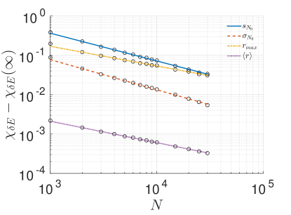
Figure 8: (Color online) The system size scaling of the support $\chi_{\delta E}=s_{N_{0}}=0.07+48N^{-0.71}$ (solid-blue) with $R^{2}=0.9997$, RMSE $=10^{-3}$, SSE $=10^{-5}$, the fluctuations (or the ETH noise) $\chi_{\delta E}=\sigma_{N_{0}}=0.02+15.5N^{-0.77}$ (dashed-red) with $R^{2}=0.9994$, RMSE $=10^{-4}$, SSE $=10^{-6}$, the maximum divergence of EEV differences from the MC prediction $\chi_{\delta E}=r_{\text{max}}=0.04+5.4N^{-0.5}$ (dashed-dotted orange) with $R^{2}=0.998$, RMSE $=10^{-3}$, SSE $=10^{-5}$ and the average EEV difference $\chi_{\delta E}=\langle r_{n}\rangle_{\delta E}=10^{-3}+0.1N^{-0.55}$ (dotted purple) with $R^{2}=0.9996$, RMSE $=10^{-6}$, SSE $=10^{-10}$ for a fixed energy interval when the interval is chosen right at the middle of the spectrum for $q_{f}=0.65$. Here $\chi_{\delta E}(\infty)$ stands for the offset value of the fitting. The RMSE and SSE stand for root mean square error and sum of squares of error, respectively.

The observation that all of the ETH indicators vanish in the thermodynamic limit for the linear regions of the spectrum implies that ETH holds, even in the strong sense because of the shrinking support Biroli et al. (2010). However this is not the case when the energy interval contains the kink region as seen in scaling plots for $q_{f}=0.65$ in Fig. 8. The scaling relation for the support shows that the support still exists in the thermodynamic limit when the kink region appears in the window. Therefore, we conclude that the kink region is composed of nonthermal states that do not vanish in the thermodynamic limit. Hence when the spectrum contains the kink region, the whole spectrum will never have a shrinking support, violating the strong form of ETH. Similarly, we observe a non-vanishing ETH noise when the kink exists in the energy interval (dashed line in Fig. 8). In literature, the fluctuations are expected to vanish away in the thermodynamic limit for the weak form of ETH to hold Biroli et al. (2010). However, we see that they do not disappear when the interval includes the kink eigenstates. This matches with the fact that we do not see thermalization when the initial state overlaps with the kink eigenstates. Therefore, we can clearly conclude that the kink eigenstates are nonthermal states that cause nonthermalization when the initial state is chosen carefully to overlap with them (Regions II and III on sudden quench maps). As a result, we argue that when the kink region exists in the spectrum ($|q|<4$) not all initial states can lead the system to thermalization even in thermodynamic limit. However due to the rarity of these nonthermal states, most of the initial states will result in thermalization (Region 1 on sudden quench map Fig. (3). Therefore, the weak form of ETH holds for $|q|<4$, and otherwise ETH holds in the strong sense (based on the shrinking support for all spectrum) since kink region disappears when we choose $|q|>4$.

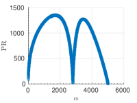
(a)

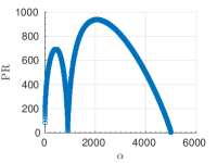
(b)

Figure 9: The participation ratio values of the eigenspectrum for a ferromagnetic Hamiltonian with (a) $q_{f}=0.5$ and (b) $q_{f}=2$ for a particle number of $10^{4}$. The eigenstates are ordered ascending in energy from the ground state ($\alpha=1$) to the most excited state.

In order to understand why there is a nonlinear structure in the EEV plot, which basically results in a nonthermal behaviour in the dynamics, we compute other quantities which can provide more information on the eigenspectrum structure of the model. The spinor Hamiltonian in Eq. (4) can actually be mapped to a single quantum-particle Hamiltonian with nearest-neighbor hopping and onsite potentials on a finite lattice. The Fock basis $\Ket{N_{-1},N_{0},N_{1}}=\{\Ket{0,N,0},\Ket{1,N-2,1},\cdots,\Ket{N/2,0,N/2}\}$ with zero total magnetization in our spinor Hamiltonian can be mapped to a basis of different lattice sites in the language of a single hopping particle in 1D lattice. Then the interaction terms $a_{0}^{\dagger}a_{0}^{\dagger}a_{1}a_{-1}$ and $a_{1}^{\dagger}a_{-1}^{\dagger}a_{0}a_{0}$ realize the nearest-neighbor hopping as can be seen when we do the operation $a_{1}^{\dagger}a_{-1}^{\dagger}a_{0}a_{0}\Ket{0,N,0}=\sqrt{N(N-1)}\Ket{1,N-2,1}$. The rest of the terms in Eq. (4) impose an onsite potential. The tight-binding Hamiltonian for the mapping could be stated as

$$H_{m} = \sum_{i=1}^{N/2-1}J(i)\left(c_{i+1}^{{\dagger}}c_{i}+\text{h.c.}\right)+\sum_{i=1}^{N/2}\eta(i)c_{i}^{{\dagger}}c_{i},$$ (13)

where $J(i)$ are real hopping coefficients that are a function of site position and $\eta(i)$ are the onsite potentials that depend on the site positions as well. The lattice size $N/2$ is the dimension of the Fock space. Here the exact dependence of $J$ and $\eta$ parameters on the positions of the sites in our imagined lattice is determined through the terms in the spinor BEC Hamiltonian Eq. (4). See App. B for how a spinor Hamiltonian engineers the lattice parameters for the mapped Hamiltonian Eq. (13). This mapping reminds us of the physics of Anderson localization Anderson (1958), albeit the onsite potentials $\eta(i)$ are not random. Hence, we study the participation ratio (PR)

$$P_{\alpha} = \left(\sum_{n=1}|\psi_{\alpha n}|^{4}\right)^{-1},$$ (14)

to analyze the localization properties of the eigenstates Evers and Mirlin (2008); Haake (2001); Canovi et al. (2011); here, $\alpha$ denotes each eigenstate and $n$ is the Fock basis vectors. As seen in Fig. 9, PR has a dip around the eigenstate corresponding to the nonthermal kink eigenstate in its corresponding EEV plot, which points to lower PR values of the nonthermal states in the Fock basis when compared to other eigenstates in the spectrum. This result hints at a link between the nonthermal behaviour that we observe in the system and the Anderson-like localization Anderson (1958) of the eigenstates in the Fock space. In other words, the nonthermal states of the system also seem to be the most localized states in the spectrum (excluding the edges).

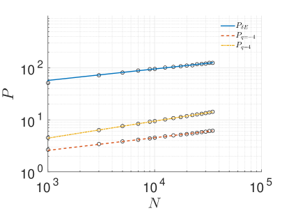
(a)

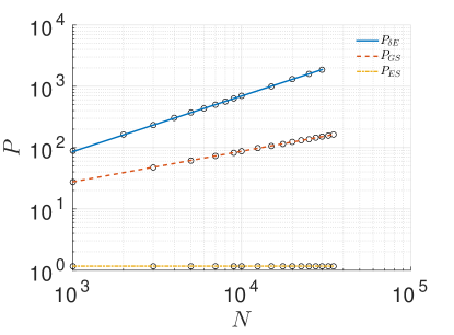
(b)

Figure 10: (Color online) System size scaling of (a) averaged participation ratio of low-PR eigenstates with a fixed energy interval of $\sim 25[c_{1}]$ around the most outlier (kink) eigenstate (solid blue), the ground state participation ratio at $q=-4$ (dashed red) and at $q=4$ (dotted-dashed orange); (b) averaged participation ratio of high-PR eigenstates with a fixed energy interval of $\sim 60[c_{1}]$ around the center of the spectrum (solid blue) when $q=3$ is chosen, PR of ground state (dashed red) and of the most-excited state (dotted-dashed orange) when the system is not going through one of its phase transition points e.g. $q=1$.

In order to make this point stronger, we analyze the system size PR scaling of eigenstates with high- and low-PR values. To target the low-PR region of the spectrum, we utilize two different methods. We emphasize that low-PR region of the spectrum in Figs. 9 (excluding the edges of the spectrum) is also the nonthermal region as already shown with the ETH indicators. There is a rapid change around the kink state which is always the extremum point of the EEV (Figs. 2c-2d) and the level spacings (Fig. 12c). Additionally the kink state slightly shifts in the spectrum as we increase the system size upto thermodynamic limit. So, even though we are able to detect the kink state in the spectrum with all these observations, we note that the kink state shows consistently low PR values for each system size but its scaling is not well-defined possibly due to finite-size effects. Therefore, the first method we apply is averaging over low-PR states around the most outlier (kink) state for each system size with a fixed energy interval. The solid line in Fig. 10a is the scaling behaviour that we observe for this method when $q=-0.65$ is chosen, which is also a $q$ value that keeps the kink state around the center of the spectrum. The extracted scaling exponent is $\gamma\propto 0.22$ with $R^{2}=0.997$. The second method employs the phase transition points. We know that the ground state is the kink eigenstate at phase transition points when $q=4$ or $q=-4$ is taken in the thermodynamic limit. Even though for a finite size condensate the phase transition points are slightly off from $q=4$ and $q=-4$ and hence the ground state is not exactly the kink eigenstate, the region around the ground state is the nonthermal kink region. This observation can be made through the difference in the PR scaling exponents of the ground state when we have $q=4$ (or $q=-4$) and $q$ is away from the phase transition points. Fig. 10b dashed line shows the scaling of the ground state when $q=1$ which we extract $P\propto N^{0.5}$ ($R^{2}=1$). The exponent $\gamma\propto 0.5$ is obtained for any $q$ sufficiently far from $q=4$ or $q=-4$. On the other hand, we obtain a scaling of $P\propto N^{0.32}(R^{2}=1)$ and $P\propto N^{0.24}(R^{2}=0.999)$ for $q=4$ and $q=-4$, respectively. Thus, clearly the ground state is neither localized nor extended completely when the system is not at its phase transition points. However, when the system goes through its phase transitions, the ground state coincides with the low-PR region states and this provides us a way to estimate the scaling exponent of states at the low-PR region. We note that extracting a well-defined scaling only for the most outlier (kink) state in a finite-size system is difficult, but still averaging over a couple of states around it gives an idea about the localization properties of the nonthermal region. Overall the extracted scaling exponents point out to that the low-PR nonthermal kink region is not completely localized region with a scaling exponent of $\gamma=0$, however it is the most localized region of the spectrum. The high-PR eigenstates that are also responsible of thermalization observed in the system show a scaling of $P_{\delta}\propto N^{0.91}$ ($R^{2}=1$), when we choose a fixed energy interval in the middle of the spectrum for Zeeman field strength $q=3$, (solid line in Fig. 10b). We observe almost the same PR scaling with exponent $\gamma=0.9$ for single eigenstates chosen at the high-PR section of the spectrum and for different $q$ values. Even though such an eigenstate is not completely extended with a scaling exponent of $\gamma=1$, it is the most extended region of the spectrum. All in all, the previous analysis of the ETH indicators clearly distinguishes the thermal and nonthermal states in the system and PR analysis demonstrates a link between localization and thermalization properties of our system, even though the thermal and nonthermal states are not completely delocalized and localized, respectively.

Finally, we note the difference between the behaviours seen in regions I and IV. Although the equilibrium behaviour in region IV can be predicted by microcanonical ensemble as seen in Fig. 6, its cause is not related to the eigenstate localization properties. We observe almost constant dynamic evolution (or almost-no nonequilibrium evolution) for the simulations at this section, which implies that one of the eigenstates dominates the evolution. In the case seen in Fig. 6, it is the most-excited state that governs the dynamics for negative $q_{f}$ values. The most-excited state shows a constant PR scaling with an exponent of $0$ (dashed-dotted line in Fig. 10b). So, even though the eigenstate is perfectly localized, the initial state is already in equilibrium with the quench Hamiltonian, which leads to the thermalization. In Fig. 6, also note that we observe thermalization for values at $q_{f}>4$ because now the initial state mostly resembles to the ground state of the quench Hamiltonian instead of the most-excited state. Finally, even though we show the PDE values at region III in Fig. 6, we should remind the reader that the dynamics of region III does not equilibrate but shows large fluctuations around its PDE value (which will be discussed in the next section as a special case).

An important difference between the spinor BEC model and the single quantum-particle hopping model is that even though the observable $\Braket{N_{0}}$ is local in the spinor BEC case, it is a non-local observable when it is mapped onto the particle lattice. However more importantly, our model does not translate to an Anderson model with random potentials. Single quantum-particle hopping model with random potentials leads to sites with very low PR values. It is also analytically known that such a model cannot cause thermalization and satisfy ETH Magán (2016). Therefore, based on our results with spinor BECs, we argue that engineering the potential of a single quantum-particle model should prevent the localization in the particle lattice and give rise to thermalization for global observables defined for this model.

IV Existence and Absence of Quantum Collapse and Revivals

In this section, we analyze the cases that demonstrate quantum collapse and revivals and derive an analytical expression to predict their time scales. Further we examine the scaling of collapse and revival times with the number of particles in the condensate to be able to present realistic predictions for the experiment. Finally we discuss ‘the special cases’, where we do not observe a revival or even equilibration.

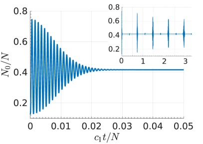
Figure 11: (Color online) The sudden quench dynamics in the short time-scale showing the collapse in detail when there is $N=2\times 10^{3}$ particles in the condensate and x-axis is scaled with the number of particles when we quench from $q_{i}=-3$ to $q_{f}=-0.5$ for the ferromagnetic case. The inset plot shows the revivals in long time-scale.

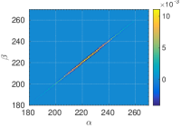
(a)

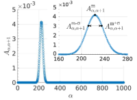
(b)

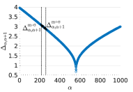
(c)

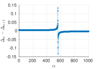
(d)

Figure 12: (Color online) (a) The overlap matrix with respect to eigenstates $\alpha$ and $\beta$, (b) the first off-diagonal terms of the overlap matrix, (c) the nearest-neighbor (NN) energy gaps and (d) The difference/derivative plot of the NN energy gaps with $N=2\times 10^{3}$ particles in the ferromagnetic condensate for the quench from $q_{i}=-3$ to $q_{f}=-0.5$. The x-axis is the eigenstates $\alpha$ ordered ascending in energy from the ground state $\alpha=1$ to the most-excited state.

Now we choose a point on the ferromagnetic sudden quench map Fig. 3 that thermalizes which can be detected via Figs. 5 and 6. So then, if we quench from $q_{i}=-3$ to $q_{f}=-0.5$, we observe a series of collapse and revivals in Fig. 11, and the equilibration value in between matches both diagonal and microcanonical ensembles. A collapse before equilibration is what mostly observed in experiments. We also intuitively expect to see a series of revivals due to the finite-size effects. However in order to understand how collapse and revivals emerge in our model, let us go back to the sudden quench procedure given in previous section and modify the Eq. (6). Notice that $c_{\alpha}^{*}c_{\beta}=c_{\beta}^{*}c_{\alpha}$ when the coefficients are real, which is the case in our problem. Also $N_{0,\alpha\beta}=N_{0,\beta\alpha}$ in our model. Then we can regroup Eq. (6) as,

$$\Braket{N_{0}(t)} = \sum_{\alpha\geq\beta}c_{\alpha}^{*}c_{\beta}\left(e^{i(E_{\alpha}-E_{\beta})t}+e^{-i(E_{\alpha}-E_{\beta})t}\right)N_{0,\alpha\beta},$$ (15)

$$= 2\sum_{\alpha\geq\beta}c_{\alpha}^{*}c_{\beta}\cos\left((E_{\alpha}-E_{\beta})t\right)N_{0,\alpha\beta}.$$

Eq. (15) tells us that dynamics we observe in a sudden quench is the interference of sinusoidal functions weighted with some overlap. We can write Eq. (15) more clearly as,

$$\Braket{N_{0}(t)} = \sum_{\alpha\geq\beta}A_{\alpha\beta}\cos\left(\Delta_{\alpha\beta}t\right),$$ (16)

where $\Delta_{\alpha\beta}=E_{\alpha}-E_{\beta}$ is the energy gaps, Fig. 12c and $A_{\alpha\beta}=2c_{\alpha}^{*}c_{\beta}N_{0,\alpha\beta}$ is the overlap matrix, Fig. 12a. We note that the diagonal terms are the most populated terms in the overlap matrix and they correspond to the diagonal ensemble prediction. In fact it is important that the off-diagonal terms vanish for thermalization to happen or they should be much smaller compared to diagonal terms. We observe this is almost the case in Fig. 12a, except the first and second off-diagonals still contribute to the dynamics even though they are much smaller than the diagonal terms. Fig. 12b shows the first off-diagonals of the overlap matrix (which we call overlap distribution in the following). This Poisson-like overlap exists when the dynamics demonstrate a series of collapse and revivals and it turns out to be important in determining the time scales of collapse and revivals in spinor condensates under SMA.

The time scale of a collapse is related to the time when the oscillating terms with an energy gap argument in Eq. (16) start to become uncorrelated. The terms corresponding to the farthest ends of the distribution are also the farthest in oscillation frequency. They become uncorrelated after all the other terms get uncorrelated. From that point on, all the oscillating terms will be destructively interfering. We estimate these elements with root-mean-square of the overlap distribution as also done for collapses in Jaynes-Cummings model Scully and Zubairy (1997). Ref. Jensen and Shankar (1985) predicts the collapse time for the Ising model as inversely proportional to the energy spread of the initial state, which is similar to our criteria and expression. The following collapse time expression produces a value of $c_{1}t_{c}/N\sim 0.02$ for the quench simulation depicted in Fig. 11:

$$t_{c} = \frac{2\pi}{|\Delta_{\alpha,\alpha+1}^{m+\sigma}-\Delta_{\alpha,\alpha+1}^{m-\sigma}|},$$ (17)

where $\Delta_{\alpha,\alpha+1}^{m}$ denotes the nearest-neighbour energy gap (level spacing, Fig. 12c) corresponding to the maximum value in the overlap distribution (Fig. 12b) and hence $\Delta_{\alpha,\alpha+1}^{m+\sigma}$ is the nearest-neighbour energy gap corresponding to the value which is $\sigma$ farther from the mean in the distribution (cf. the inset of Fig. 12b). It is possible to fine-tune the predicted collapse time by taking more than $1\sigma$ of the overlap distribution. Also note that we find $c_{1}t_{c}\sim N^{1/2}$ as the scaling of the collapse time-scale.

A quantum revival happens when all the oscillating terms become correlated with each other again. This can be measured through the difference between nearest-neighbour energy gaps corresponding to the the mean $\Delta_{\alpha,\alpha+1}^{m}$ and the closest point to mean $\Delta_{\alpha,\alpha+1}^{m-1}$ in the overlap distribution (cf. the inset of Fig. 12b),

$$t_{r} = \frac{2\pi}{|\Delta_{\alpha,\alpha+1}^{m}-\Delta_{\alpha,\alpha+1}^{m-1}|}.$$ (18)

Fig. 12d shows the differences between nearest-neighbour energy gaps. Note that $\Delta_{\alpha}-\Delta_{\alpha+1}$ are mostly flat around where the overlap distribution is nonzero. This is vital for a collective revival to occur, since otherwise terms in Eq. (16) will never constructively interfere at a fixed time, namely the revival time. When we have $t_{r}(\Delta_{\alpha}-\Delta_{\alpha+1})=2\pi$, all oscillating terms interfere constructively, creating the first revival. Both the analytical expression and the data analysis give a revival time $c_{1}t_{r}/N\sim 0.735$. Since the scaling of the revival time-scale turns out to be $c_{1}t_{r}\sim N$, this value can be obtained for all sizes for the parameters depicted in Fig. 11. Also note that the linearly growing recurrence times is well-known in the literature Eisert et al. (2015). The small peaks between the collapse and revivals seen in Fig. 11 are the small revivals contributed by the second off-diagonal terms in the overlap matrix, Fig. 12a. We can also predict the oscillation frequency,

$$t_{\text{osc}} = \frac{2\pi}{\Delta_{\alpha,\alpha+1}^{m}},$$ (19)

by using the nearest-neighbor energy gap at the maximum point of the overlap distribution $\Delta_{\alpha,\alpha+1}^{m}$. There is an another interesting quantity that can be predicted in a collapse-revival picture. We observe how revivals are suppressed in a very long time scale in the inset of Fig. 11. This ‘randomizing time’ is where the initial memory of the system irreversibly gets lost. Even though a typical randomizing time is out of experimental reach, it is interesting to note that an isolated, unitary and finite-size quantum system will be eventually randomized and hence completely thermalized at the randomizing time which can be estimated via

$$t_{rz} = \frac{2\pi}{|\Delta^{\prime}_{m+\sigma}-\Delta^{\prime}_{m-\sigma}|},$$ (20)

where $\Delta^{\prime}=\Delta_{\alpha}-\Delta_{\alpha+1}$ denotes the difference between nearest-neighbor energy gaps (Fig. 12d) and the rest of the notation is same with the previous definitions where we use the overlap distribution for $m\pm\sigma$.

In order to give a sense of these time scales, let us fix the particle density in our condensate to $5\times 10^{14}$ cm^-3. Then the coefficient reads $c_{1}\sim-2\pi\times 9$ Hz, which gives a realistic collapse time of $\sim 0.5$ s and a revival time of $\sim 25$ s for a condensate particle number of $2\times 10^{3}$.

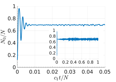
(a)

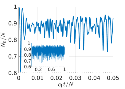
(b)

Figure 13: (Color online) The sudden quench dynamics in short time-scale (a) from $q_{i}=-3$ to $q_{f}=0.5$ and (b) from $q_{i}=4.1$ to $q_{f}=2$ with insets of long time-scales for ferromagnetic condensates and $N=2\times 10^{3}$ particles.

This sudden quench experiment corresponds to a data point on Fig. 5, where ETH can explain the match between the thermal relaxation values predicted by diagonal ensemble and microcanonical ensemble. Therefore we can conclude that there is thermalization until the initial memory of the system comes back with a quantum revival.

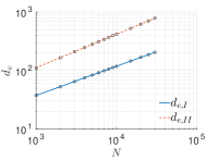
(a)

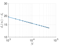
(b)

Figure 14: (Color online) The effective dimension scaling for a quench (a) from $q_{i}=-3$ to $q_{f}=0.5$ (Region II) (dashed red) with $d_{e}\propto N^{0.57}$, from $q_{i}=-3$ to $q_{f}=-0.5$ (Region I) (solid blue) with $d_{e}\propto N^{0.5}$ and (b) from $q_{i}=4.1$ to $q_{f}=2$ (Region III) with $d_{e}=28.3-36.3N^{-0.092}$ with respect to system size. The correlation coefficient is $R^{2}=1$ for all figures. $d_{e}(\infty)$ stands for the offset value of the fitting in subfigure b.

Then it is important to see how the times of the collapse and the first revival scale with the number of particles in the condensate. Reminding the reader of $c_{1}t_{c}\sim N^{1/2}$ and $c_{1}t_{r}\sim N$ and using the estimations done for Thomas-Fermi limit in Ref. Pu et al. (1999), we figure out that $c_{1}\sim N^{2/3}$ in 1-dimension, hence $t_{c}\sim N^{-1/6}$ and $t_{r}\sim N^{1/3}$. Although SMA breaks down in large condensate limit Pu et al. (1999) and the experiments always have finite sizes, it is still insightful to imagine the thermodynamic limit $N\rightarrow\infty$. In thermodynamic limit, a 1D spinor BEC system has a diverging revival time and a vanishing collapse time, which implies thermalization described by ETH for our model.

Now let us choose a point on the map Fig. 3 that does not thermalize to illustrate one of the special cases. If we quench from $q_{i}=-3$ to $q_{f}=0.5$ (corresponding to the parameters in Fig. 2a and 2c), we observe the dynamical behaviour in Fig. 13a. There is a well-defined collapse whose time-scale can be predicted with the collapse criterion and the system seems to equilibrate right after the collapse. However looking at the dynamics for a longer time (inset of Fig. 13a) reveals that the revivals attempt to happen at different times resulting with no collective recurrence for a finite system. This is due to the broad shape of the EON window (Fig. 2a). One can calculate the so-called effective dimension of the system Reimann (2008); Short (2011) under this specific quench, which is the participation ratio of the initial state in the eigenstate reference basis instead of Fock basis,

$$d_{e} = \left(\sum_{\alpha}|c_{\alpha}|^{4}\right)^{-1},$$ (21)

where $|c_{\alpha}|^{2}$ is the eigenstate occupation numbers as in Eq. (5). The effective dimension is a measure of how broad the EON window is. In order to determine if a quantum system equilibrates, one needs to look at the scaling of the effective dimension with the system size. We find a scaling of $d_{e}\propto N^{0.57}$ ($R^{2}=1$) for this quench (Fig. 14a) and in fact almost the same exponent for any other quench in region II of the sudden quench map. Therefore, we argue that in thermodynamic limit the effective dimension diverges $d_{e}\rightarrow\infty$ as $N\rightarrow\infty$, which leads the system to equilibration. For a comparison with region I, we calculated the effective dimension of a region I quench from $q_{i}=-3$ to $q_{f}=-0.5$ which is already shown to thermalize and hence equilibrate. As seen in Fig. 14b, the effective dimension is found to be $d_{e}\propto N^{0.5}$ ($R^{2}=1$) and this scaling exponent is universal for all the quenches in region I. Hence, the previous argument follows. If we return to the discussion on region II dynamical behaviour, the overlap distribution (first off-diagonals in the overlap matrix) is similar in shape with Fig. 2a. Further computations show that the energy gap differences between neighbouring terms in the overlap distribution are different and hence they give rise to different revival times (see. Eq. 18 and Fig. 12d around the kink region) confirming the dynamical response. Also clearly the EON for this point on the map (Fig. 2a) is not narrow enough to avoid the kink nonthermal states, which causes nonthermalization for the system. As a result, the system only equilibrates with no collective recurrence for any finite dimensions of the system. Also note that as we increase the system size, the time-scale of the revival attempts diverges which leaves us with the equilibrated section seen right after the decay. This is the behaviour that we observe for the region II on sudden quench map Fig. 3.

The second special point on the map Fig. 3 is a quench from $q_{i}=4.1$ to $q_{f}=2$, which demonstrates the behaviour for region III on Fig. 3. Fig. 13b shows oscillatory behaviour around the system’s PDE value for all times without any collapse or revival. The overlap distribution looks like Fig. 2b, however differently the first off-diagonal terms are not really smaller than the diagonal terms (EON of the system) and in fact second and third off-diagonal terms in the overlap matrix $A_{\alpha\beta}$ substantially contribute to the dynamics, too. This is in fact why we observe large fluctuations (Eq. 16). The scaling of the effective dimension for this quench turns out to be $d_{e}\propto 28.3-36.3N^{-0.092}$ ($R^{2}=1$), which implies that in thermodynamic limit $d_{e}\rightarrow 28.3$ while $N\rightarrow\infty$ and the effective dimension is going to saturate at a constant value (Fig. 14b). This will lead to nonequilibration since the effective dimension will be so much smaller than the dimension of the Hilbert space, $d_{e}\ll d_{H}=\infty$. We note that all quenches on region III shows a universal scaling exponent with slightly different scaling parameters. As a final remark, the EON window is narrow enough to coincide only with the nonthermal kink states implying the PDE of the system is not the thermal prediction.

V Conclusions and Discussion

Spinor BEC model with SMA has an eigenstate expectation value spectrum for the observable $\Braket{N_{0}}$ (the number of particles with spin-0 component in the condensate) that shows thermalization in the context of eigenstate thermalization hypothesis in the weak form when the quadratic Zeeman term is $|q|<4$ due to the ‘rare’ nonthermal states and in the strong form, otherwise. We adopted widely used ETH indicators to obtain our results, e.g. support, ETH noise (fluctuations), maximum divergence from the microcanonical prediction for an eigenstate in a fixed energy interval and the EEV differences. We studied the effect of these nonthermal states in the spectrum by driving the system out of equilibrium via a sudden quench from the ground state of an initial Hamiltonian with $q_{i}$ to a final Hamiltonian with $q_{f}$. Even though this procedure allowed us to study certain initial conditions, we are able to generalize the results and predict the behaviour of the system with an arbitrary initial condition. On the other hand, such a procedure is experimentally realizable and we have shown that it leads to a classification scheme of the system dynamics: the sudden quench maps, Figs. 3 and 4. Sudden quench maps give us the prediction of diagonal ensemble in the long-time limit or the long-time average of the dynamical response. For a region when the system does not equilibrate (e.g. Region III), the value on the map is the average of the response.

We observed that ETH is satisfied in region I with well-defined collapse and revivals where the revival time-scale is out of reach for realistic condensate sizes. For the region II, the dynamics equilibrate around a nonthermal value right after a collapse (shown via the scaling of effective dimension) due to the effect of nonthermal rare states in the spectrum. Even though dynamics at region II shows attempts for a quantum revival, not all the oscillating terms become correlated at the same time, implying the lack of a clear quantum revival. We interpreted the thermalization seen for the region I as weak ETH, because even though the initial state does not overlap with the rare nonthermal states (kink region), these states still exist in the spectrum, even in the thermodynamic limit. Therefore, clearly not all initial states are able to thermalize the system. In fact, region II is an example of these cases. However, for the Hamiltonians with $|q|>4$, the kink region does not exist in the spectrum even for finite-size condensates. Thus, we conclude that ETH holds in the strong sense for this set of Hamiltonians.

The system for the region III does not equilibrate or show any collapse-revival phenomena and instead oscillates, because the effective dimension saturates at a finite value whereas the Hilbert space dimension diverges in the thermodynamic limit and the main contribution to the dynamics comes from nonthermal states which also have low participation ratio values in the Fock basis. We explicitly showed that the thermal and nonthermal states in the spectrum have high and low PR values with system-size scaling exponents of $\sim 0.9$ and $\sim 0.2$, respectively. In the end, thermalization seems to be linked to the localization properties of the eigenstates. In region IV, the system thermalizes with very small amplitude collapse and revivals either at $0$ or $1$. The initial state is already in almost-equilibrium with the quench Hamiltonian, leading to almost-no nonequilibrium evolution for the system to pursue. For the anti-ferromagnetic sudden quench map Fig. 4, we always observe only the regions III and IV given that the initial state is a ground state of an anti-ferromagnetic Hamiltonian. Finally, we note that the region around $q_{f}\sim 0$ on both sudden quench maps is special in terms of how the thermalization value is independent of the initial state chosen. This behaviour is expected, because almost all of the eigenstates in the spectrum contribute to the observable expectation value in the same amount regardless of the system size.

Interpretation of sudden quench maps as non-equilibrium phase diagrams and the transitions between regions as the dynamical phase transitions seems possible given that these dynamical transition points originate from the equilibrium quantum phase transitions of the system. We leave the question if these transitions can be related to dynamical quantum phase transitions (DQPTs) Heyl (2017) as an investigation for future.

Spinor Bose-Einstein condensates are relatively more convenient to experiment with Jiang et al. (2014); Liu et al. (2009); Anquez et al. (2016); Stamper-Kurn and Ueda (2013); Hoang et al. (2016) and numerically less costly (when SMA is applied), compared to more popular models such as Bose-Hubbard model or Ising models. Here, we showed that spinor BECs can also be used as a test-bench to test the ideas on the thermalization of isolated quantum systems.

Appendix A Microcanonical Window Selection

The microcanonical ensemble (MC) prediction should not depend on the size of the energy window. This constraint prevents us to calculate the MC prediction for the cases where the kink structure exists in the spectrum and the initial state is chosen in such a way that it overlaps with the kink. See Figs. 5 and 6 for these regions where the MC energy interval cannot be well-defined. This result is consistent with the condition Eq. 8 which does not hold for the aforementioned cases above. However the typical eigenstates of a spinor BEC system are thermal with high PR values and therefore we can compare the prediction of diagonal ensemble (PDE) (or the long-time average of dynamical response) with the MC prediction for almost any initial state.

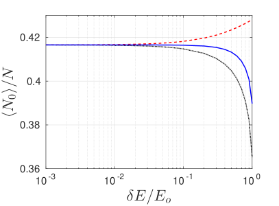
Figure 15: (Color online) The microcanonical ensemble thermal prediction with respect to different energy intervals for $[E_{o}-\delta E,E_{o}]$ (red-dashed), $[E_{o}-\delta E,E_{o}+\delta E]$ (blue-solid) and $[E_{o},E_{o}+\delta E]$ (black-dotted) when a sudden quench is applied from $q_{i}=-3$ to $q_{f}=-0.5$ for a condensate size of $N=10^{4}$.

For these cases, we calculate the mean energy of the system according to

$$E_{o} = \sum_{\alpha}|C_{\alpha}|^{2}E_{\alpha},$$ (22)

where $E_{\alpha}$ is the energy associated with each eigenstate. Keeping in mind that the energy window should be much smaller than the mean energy $\delta E\ll E_{o}$, we look for the threshold window size $\delta E_{\text{th}}$ that starts to affect the MC prediction. Then any $\delta E<\delta E_{\text{th}}$ gives a well-defined MC energy window. We also compare three different possibilities for the window size as $[E_{o}-\delta E,E_{o}]$, $[E_{o}-\delta E,E_{o}+\delta E]$ and $[E_{o},E_{o}+\delta E]$. Fig. 15 shows an example of this procedure.

Appendix B Mapping of a Spinor Hamiltonian onto a Single Quantum-Particle Hopping Model

Here we show how the parameters of single quantum-particle model (Eq. (13)) depend on the sites of the lattice. Upon comparing with the spinor Hamiltonian Eq. (4), we observe that the Zeeman field strength $q$ modifies only the diagonal terms and hence the onsite potential terms $\eta$. Therefore, the single particle Hamiltonian family that can produce the dynamics in this paper consists of only different onsite potential configurations.

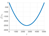
(a)

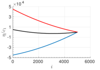
(b)

Figure 16: (Color online) (a) The hopping parameter $J$ for the mapped single particle model, (b) the onsite potential parameter $\eta$ for a condensate model with Zeeman field strength $q=4.5$ (blue-lower curve), $q=-0.5$ (black middle curve) and $q=-4.5$ (red upper curve) with respect to site position $i$ for a condensate of size $N=10^{4}$.

Fig. 16a shows the hopping coefficients with respect to single particle lattice positions. This functional dependence of $J$ onto the site positions is fixed for each spin-1 BEC Hamiltonian. Fig. 16b shows different onsite potential configurations depending on the Zeeman field strength. The most important observation is that onsite potentials for all cases are not random, instead they are engineered potentials with respect to site positions. This property breaks the localization of single particle hopping model and hence we observe thermalization of an observable that is nonlocal for the model.

References

- Fialko and Hallwood (2012) O. Fialko and D. W. Hallwood, Phys. Rev. Lett. 108, 085303 (2012).
- Fialko (2015) O. Fialko, Phys. Rev. E 92, 022104 (2015).
- Kaufman et al. (2016) A. M. Kaufman, M. E. Tai, A. Lukin, M. Rispoli, R. Schittko, P. M. Preiss, and M. Greiner, Science 353, 794 (2016).
- Neill et al. (2016) C. Neill, P. Roushan, M. Fang, Y. Chen, M. Kolodrubetz, Z. Chen, A. Megrant, R. Barends, B. Campbell, B. Chiaro, A. Dunsworth, E. Jeffrey, J. Kelly, J. Mutus, P. J. J. O’Malley, C. Quintana, D. Sank, A. Vainsencher, J. Wenner, T. C. White, A. Polkovnikov, and J. M. Martinis, Nature Physics 12, 1037 (2016), arXiv:1601.00600 [quant-ph] .
- Nandkishore and Huse (2015) R. Nandkishore and D. A. Huse, Annual Review of Condensed Matter Physics 6, 15 (2015).
- Huse et al. (2013) D. A. Huse, R. Nandkishore, V. Oganesyan, A. Pal, and S. L. Sondhi, Phys. Rev. B 88, 014206 (2013).
- von Neumann (2010) J. von Neumann, The European Physical Journal H 35, 201 (2010).
- Deutsch (1991) J. M. Deutsch, Phys. Rev. A 43, 2046 (1991).
- Srednicki (1994) M. Srednicki, Phys. Rev. E 50, 888 (1994).
- Jensen and Shankar (1985) R. V. Jensen and R. Shankar, Phys. Rev. Lett. 54, 1879 (1985).
- Rigol et al. (2008) M. Rigol, V. Dunjko, and M. Olshanii, Nature 452, 854 (2008).
- Polkovnikov et al. (2011) A. Polkovnikov, K. Sengupta, A. Silva, and M. Vengalattore, Rev. Mod. Phys. 83, 863 (2011).
- Fermi et al. (1955) E. Fermi, J. Pasta, and S. Ulam, Document LA-1940 (May 1955).
- Rigol et al. (2007) M. Rigol, V. Dunjko, V. Yurovsky, and M. Olshanii, Phys. Rev. Lett. 98, 050405 (2007).
- Tabor (1989) M. Tabor, Chaos and integrability in nonlinear dynamics: an introduction, Wiley-Interscience publication (Wiley, 1989).
- Romano and de Passos (2004) D. R. Romano and E. J. V. de Passos, Phys. Rev. A 70, 043614 (2004).
- Zhang et al. (2005) W. Zhang, D. L. Zhou, M.-S. Chang, M. S. Chapman, and L. You, Phys. Rev. A 72, 013602 (2005).
- Jaynes (1957) E. T. Jaynes, Phys. Rev. 106, 620 (1957).
- Gogolin et al. (2011) C. Gogolin, M. P. Müller, and J. Eisert, Phys. Rev. Lett. 106, 040401 (2011).
- Manmana et al. (2007) S. R. Manmana, S. Wessel, R. M. Noack, and A. Muramatsu, Phys. Rev. Lett. 98, 210405 (2007).
- Kollath et al. (2007) C. Kollath, A. M. Läuchli, and E. Altman, Phys. Rev. Lett. 98, 180601 (2007).
- Shiraishi and Mori (2017) N. Shiraishi and T. Mori, Phys. Rev. Lett. 119, 030601 (2017).
- Biroli et al. (2010) G. Biroli, C. Kollath, and A. M. Läuchli, Phys. Rev. Lett. 105, 250401 (2010).
- Ikeda et al. (2013) T. N. Ikeda, Y. Watanabe, and M. Ueda, Phys. Rev. E 87, 012125 (2013).
- Alba (2015) V. Alba, Phys. Rev. B 91, 155123 (2015).
- Kim et al. (2014) H. Kim, T. N. Ikeda, and D. A. Huse, Phys. Rev. E 90, 052105 (2014).
- Pal and Huse (2010) A. Pal and D. A. Huse, Phys. Rev. B 82, 174411 (2010).
- Yurovsky and Olshanii (2011) V. A. Yurovsky and M. Olshanii, Phys. Rev. Lett. 106, 025303 (2011).
- Canovi et al. (2011) E. Canovi, D. Rossini, R. Fazio, G. E. Santoro, and A. Silva, Phys. Rev. B 83, 094431 (2011).
- Evers and Mirlin (2008) F. Evers and A. D. Mirlin, Rev. Mod. Phys. 80, 1355 (2008).
- Anderson (1958) P. W. Anderson, Phys. Rev. 109, 1492 (1958).
- Scully and Zubairy (1997) M. Scully and M. Zubairy, Quantum Optics (Cambridge University Press, 1997).
- Will et al. (2010) S. Will, T. Best, U. Schneider, L. Hackermüller, D.-S. Lühmann, and I. Bloch, Nature 465, 197 (2010).
- Greiner et al. (2002) M. Greiner, O. Mandel, T. W. Hänsch, and I. Bloch, Nature 419, 51 (2002).
- Bocchieri and Loinger (1957) P. Bocchieri and A. Loinger, Phys. Rev. 107, 337 (1957).
- Law et al. (1998) C. K. Law, H. Pu, and N. P. Bigelow, Phys. Rev. Lett. 81, 5257 (1998).
- Pu et al. (2000) H. Pu, C. Law, and N. Bigelow, Physica B: Condensed Matter 280, 27 (2000).
- Pu et al. (1999) H. Pu, C. K. Law, S. Raghavan, J. H. Eberly, and N. P. Bigelow, Phys. Rev. A 60, 1463 (1999).
- Stamper-Kurn and Ueda (2013) D. M. Stamper-Kurn and M. Ueda, Rev. Mod. Phys. 85, 1191 (2013).
- Sadler et al. (2006) L. E. Sadler, J. M. Higbie, S. R. Leslie, M. Vengalattore, and D. M. Stamper-Kurn, Nature 443, 312 (2006).
- Zhang and Duan (2013) Z. Zhang and L.-M. Duan, Phys. Rev. Lett. 111, 180401 (2013).
- Zhang et al. (2003) W. Zhang, S. Yi, and L. You, New Journal of Physics 5, 77 (2003).
- Jiang et al. (2014) J. Jiang, L. Zhao, M. Webb, and Y. Liu, Phys. Rev. A 90, 023610 (2014).
- Yi et al. (2002) S. Yi, O. E. Müstecaplıoğlu, C. P. Sun, and L. You, Phys. Rev. A 66, 011601 (2002).
- Luo et al. (2017) X.-Y. Luo, Y.-Q. Zou, L.-N. Wu, Q. Liu, M.-F. Han, M. K. Tey, and L. You, Science 355, 620 (2017).
- Liu et al. (2009) Y. Liu, S. Jung, S. E. Maxwell, L. D. Turner, E. Tiesinga, and P. D. Lett, Phys. Rev. Lett. 102, 125301 (2009).
- Hoang et al. (2016) T. M. Hoang, H. M. Bharath, M. J. Boguslawski, M. Anquez, B. A. Robbins, and M. S. Chapman, Proceedings of the National Academy of Sciences 113, 9475 (2016).
- Anquez et al. (2016) M. Anquez, B. A. Robbins, H. M. Bharath, M. Boguslawski, T. M. Hoang, and M. S. Chapman, Phys. Rev. Lett. 116, 155301 (2016).
- Zunkovic et al. (2016) B. Zunkovic, M. Heyl, M. Knap, and A. Silva, ArXiv e-prints (2016), arXiv:1609.08482 [cond-mat.quant-gas] .
- Zhang et al. (2017) J. Zhang, G. Pagano, P. W. Hess, A. Kyprianidis, P. Becker, H. Kaplan, A. V. Gorshkov, Z.-X. Gong, and C. Monroe, ArXiv e-prints (2017), arXiv:1708.01044 [quant-ph] .
- Rigol (2009) M. Rigol, Phys. Rev. Lett. 103, 100403 (2009).
- Kardar (2007) M. Kardar, Statistical Physics of Particles (Cambridge University Press, 2007).
- (53) V. Dunjko and M. Olshanii, “Thermalization from the perspective of eigenstate thermalization hypothesis,” in Annual Review of Cold Atoms and Molecules, pp. 443–471.
- Srednicki (1996) M. Srednicki, Journal of Physics A: Mathematical and General 29, L75 (1996).
- Haake (2001) F. Haake, Quantum Signatures of Chaos, Physics and astronomy online library (Springer, 2001).
- Magán (2016) J. M. Magán, Phys. Rev. Lett. 116, 030401 (2016).
- Eisert et al. (2015) J. Eisert, M. Friesdorf, and C. Gogolin, Nature Physics 11, 124 (2015).
- Reimann (2008) P. Reimann, Phys. Rev. Lett. 101, 190403 (2008).
- Short (2011) A. J. Short, New Journal of Physics 13, 053009 (2011).
- Heyl (2017) M. Heyl, ArXiv e-prints (2017), arXiv:1709.07461 [cond-mat.stat-mech] .