Traveling dark-bright solitons in a reduced spin-orbit coupled system:
application to Bose-Einstein condensates

Abstract

In the present work, we explore the potential of spin-orbit (SO) coupled Bose-Einstein condensates to support multi-component solitonic states in the form of dark-bright (DB) solitons. In the case where Raman linear coupling between components is absent, we use a multiscale expansion method to reduce the model to the integrable Mel’nikov system. The soliton solutions of the latter allow us to reconstruct approximate traveling DB solitons for the reduced SO coupled system. For small values of the formal perturbation parameter, the resulting waveforms propagate undistorted, while for large values thereof, they shed some dispersive radiation, and subsequently distill into a robust propagating structure. After quantifying the relevant radiation effect, we also study the dynamics of DB solitons in a parabolic trap, exploring how their oscillation frequency varies as a function of the bright component mass and the Raman laser wavenumber.

I Introduction

The subject of atomic Bose-Einstein condensates (BECs) has experienced numerous experimental and theoretical developments over the past two decades. These developments have been summarized not only in numerous books stringari ; pethick ; emergent ; siambook ; proukbook ; ldcbook , but also in special volumes dedicated to the subject romrep . Within this theme, numerous more specialized topics have emerged over time that have attracted considerable attention. One of the most recent and intensely investigated ones, concerns the realization of spin-orbit (SO) coupling for neutral atoms in BECs spiel1 ; expcol (see also Ref. ho for theoretical work), as well as fermionic gases fermi1 ; fermi2 . In this context, there have been experiments exploring fundamental phenomena; these include the phase transition from a miscible to an immiscible superfluid spiel1 , the divergence of spin-polarization susceptibility during the transition from a non-magnetic to a magnetic ground state expcol , the observation of Zitterbewegung oscillations zbengels ; zbspiel , the demonstration of Dicke-type phase transitions engdicke , and the manipulation of the interplay between dispersion and nonlinearity to induce negative effective mass, dynamical instability and nonlinear wave formation engbusch , among others. At this stage, numerous works combining the efforts of experimental and theoretical groups have summarized some of the principal developments in the field, both at the early stages dalib ; spiel3 ; revspiel , as well as more recently engreview .

On the other hand, there has been considerable progress towards exploring the dynamics of coherent nonlinear structures, in the form of vector solitons, in multi-component repulsive BECs (including pseudo-spinor and spinor ones) –cf. the recent review revip . A principal structure that has been studied in numerous related experimental studies has been the dark-bright (DB) soliton hamburg ; pe1 ; pe2 ; pe3 ; azu , the closely related (i.e., emerging from an SO$(2)$ rotation) dark-dark soliton pe4 ; pe5 and, more recently, the so-called dark-antidark soliton antidark (below, we use the term “soliton” in a loose sense, without implying complete integrability mja ). An important characteristic of the DB soliton structure is that the bright soliton component cannot be supported on its own in such repulsive BECs, yet it arises due to the waveguiding/trapping induced by the dark soliton component of the DB soliton pair. It should also be mentioned here that such states have been previously pioneered in nonlinear optics, where single and multiple ones such were experimentally realized in photorefractive crystals seg1 ; seg2 . Very recently, generalization of these structures in three-components, in the form of dark-dark-bright and bright-bright-dark solitons, were experimentally observed in $F=1$ spinor BECs useng (see also Ref. usspin for relevant theoretical predictions).

Vector solitons have also been studied in the context of SO coupled BECs. In particular, in the one-dimensional (1D) setting, solitonic structures of the bright prl14 ; ch1 or dark usepl ; vasos1 types –as well as gap solitons gap1 ; gap2 ; gap3 in BECs confined in optical lattices– were predicted to occur, and their dynamics was studied b1 . In fact, the presence of SO coupling enriches significantly the possibilities regarding the structural form of solitons, as well as their stability and dynamical properties. Examples include the prediction of structures composed by embedded families of bright, twisted or higher excited solitons inside a dark soliton, that occupy both energy bands of the spectrum of a SO coupled BEC and performing Zitterbewegung oscillations vasos1 , or the possibility for effective negative mass bright (dark) solitons that can be formed in SO coupled BECs with repulsive (attractive) interactions nmass (note that such a change of sign in the effective mass, i.e., the possibility of “dispersion management” for SO coupled BECs was later demonstrated in the experimental work of Ref. engbusch ). In addition, the existence of quasiscalar soliton complexes due to a localized SO coupling-induced modification of the interaction forces between solitons v1 , or of freely moving solitons in spatially inhomogeneous BECs with helicoidal SO coupling v2 , was also reported. We also note in passing that, in higher-dimensional settings, stable solitons –composed by mixed fundamental and vortical components– were found in free 2D bam1 and 3D bam2 space; these structures are supported by the attractive cubic nonlinearity, without the help of any trapping potential (see also Ref. bam3 and Refs. bam4 ; bam5 for relevant work in dipolar BECs, as well as the recent review d1 ).

In the present work, motivated by the developments in the study of DB solitons in pseudo-spinor condensates, we will attempt to identify such structures in SO coupled BECs. In the relevant process, there is a nontrivial “impediment”, namely a Raman coupling –represented by a Rabi-type linear coupling, of strength $\Omega_{R}$– between the two SO-coupled BEC components. Such a coupling, is known to result in population exchange between components, such that the difference of the two condensate populations oscillates at frequency $2\Omega_{R}$ rab . This naturally enforces a similar background state between the two components, which would not allow the formation of the DB soliton state (recall that the dark soliton is formed on top of a background wave, while the bright one assumes trivial boundary conditions kivsharagr ).

Here, we will thus study the problem under the assumption that the Rabi coupling is absent. In fact, the only term that we will consider as acting will be the one associated with the wavenumber of the Raman laser, which couples the two components imposing in the relevant vector nonlinear Schrödinger (NLS) [Gross-Pitaevskii (GP) equation in the BEC context] a Dirac-like coupling –cf., e.g., Ref. prl14 . Such a “reduced SO coupled system”, constitutes a vectorial NLS model that also finds applications in nonlinear optics, where it describes the interaction of two waves of different frequencies in a dispersive nonlinear medium kivsharagr ; rysk . Our approach in this effort will be based on developing a multiscale expansion technique, to transform the original nonintegrable model to another, integrable one, facilitating the study of the former on the basis of the connection to the latter. Such multiscale expansion methods are usually employed in studies on the existence, stability and dynamics of solitons both in nonlinear optics and BECs (see the reviews kivsharagr ; dep and nonlin ; jpa respectively, and references therein). Here, our perturbative approach reveals that, in the small-amplitude limit, DB soliton solutions of the reduced SO system do exist, and can be well approximated by the soliton solutions of the completely integrable Mel’nikov system Mel1 ; Mel2 . Our analytical predictions will then be tested numerically, with and without a trap (in the latter, we will examine the oscillatory dynamics of the DB solitons), as well as within or outside the range of expected validity of the theory.

Our presentation will be structured as follows. In section II, we will introduce the model and present our analytical results based on the multiscale expansion method. Section III, is devoted to the presentation of numerical results, where we will examine in particular the range of validity of our analytical approximations. Finally, in section IV, we will summarize our findings and present our conclusions, suggesting also possible directions of extension of the present program towards future studies.

II Model and its analytical consideration

II.1 Mean-field model for spin-orbit coupled condensates

We consider a quasi-1D SO coupled BEC, confined in a trap with longitudinal and transverse frequencies, $\omega_{x}$ and $\omega_{\perp}$, such that $\omega_{x}\ll\omega_{\perp}$. In the framework of mean-field theory, and in the case of equal contributions of Rashba ras and Dresselhaus dres SO couplings (as in the experiment spiel1 ), this system is described by the energy functional spiel1 ; ho :

$$\mathcal{E}\!=\!\mathbf{u}^{\dagger}\mathcal{H}_{0}\mathbf{u}+\frac{1}{2}\left(g_{11}|u|^{4}+g_{22}|v|^{4}+2g_{12}|u|^{2}|v|^{2}\right),$$ (1)

where $\mathbf{u}\equiv(u,v)^{T}$, and the condensate wavefunctions $u$ and $v$ are the two pseudo-spin components of the BEC. Furthermore, the single particle Hamiltonian $\mathcal{H}_{0}$ in Eq. (1) reads:

$$\mathcal{H}_{0}=\frac{1}{2m}(\hat{p}_{x}+k_{L}\hat{\sigma}_{z})^{2}+V(x)+\Omega_{R}\hat{\sigma}_{x}+\delta\hat{\sigma}_{z},$$ (2)

where $\hat{p}_{x}=-i\hbar\partial_{x}$ is the momentum operator in the longitudinal direction, $m$ is the atomic mass, and $\hat{\sigma}_{x,z}$ are the Pauli matrices. The SO coupling terms are characterized by the following parameters: the wavenumber $k_{L}$ of the Raman laser which couples the two components, the strength of the coupling $\Omega_{R}$, and a possible energy shift $\delta$ due to detuning from the Raman resonance; below, our analysis will be performed in the case of $\delta=0$ (see also discussion below).

Here, it should be noted that upon expanding the squared term in the first part of the single atom Hamiltonian (2), it is clear that a term $\sim k_{L}\hat{p}_{x}\hat{\sigma}_{z}$ appears, which describes the velocity mismatch between the two components, equal to $2k_{L}$. The physical origin of this term is due to the fact that the two Raman laser beams couple atoms having different velocities. Such a velocity mismatch between different field components is also typical in nonlinear optics, e.g., in the case of interaction between two waves of the same polarization but of different frequencies in a nonlinear dispersive medium rysk (see also Ref. kivsharagr and discussion below).

In addition, the external trapping potential $V(x)$, is assumed to be of the usual parabolic form, $V=(1/2)m\omega_{x}^{2}x^{2}$. Finally, the effective 1D coupling constants $g_{ij}$ are given by $g_{ij}=2\hbar\omega_{\perp}\alpha_{ij}$, where $\alpha_{ij}$ are the s-wave scattering lengths. Below, we will present results for repulsive ($\alpha_{ij}>0$) interatomic interactions; furthermore, since in the typical case of ⁸⁷Rb atoms spiel1 the ratios of the scattering lengths are $\alpha_{11}:\alpha_{12}:\alpha_{22}=1:0.995:0.995$, we will use the physically relevant approximation of equal scattering lengths, namely $\alpha_{11}\approx\alpha_{12}\approx\alpha_{22}=\alpha$.

It is also important to discuss here the versatility of the Hamiltonian (2) with respect to the different parameters. The SO coupling is characterized by a strength $k_{L}$, which only depends on the laser wavelength $\lambda_{L}$ and the relative angle between the counter-propagating beams; thus, by changing the geometry of the lasers, one can control the SO interactions. Additionally, the Rabi oscillation frequency $\Omega_{R}$ depends on the laser beam intensity, which can also be controlled, while the energy difference $\delta$ can be easily tuned by changing the relative frequency of the counter-propagating lasers. Thus, unlike the SO coupling in condensed matter and electron systems where such a coupling is an intrinsic property of the material ras ; dres , in the context of BECs this coupling can be accurately controlled by different external parameters dalib ; spiel3 ; revspiel .

Using Eq. (1), we can obtain the following dimensionless equations of motion:

$$iu_{t} = \left(-\frac{1}{2}\partial^{2}_{x}-\frac{i}{2}\epsilon\partial_{x}+V(x)+|u|^{2}+|v|^{2}\right)u+\Omega_{R}v,$$ (3)

$$iv_{t} = \left(-\frac{1}{2}\partial^{2}_{x}+\frac{i}{2}\epsilon\partial_{x}+V(x)+|u|^{2}+|v|^{2}\right)v+\Omega_{R}u,$$ (4)

where subscripts denote partial derivatives, while energy, length, time and densities are measured in units of $\hbar\omega_{\perp}$, $a_{\perp}$ (which is equal to $\sqrt{\hbar/m\omega_{\perp}}$), $\omega_{\perp}^{-1}$, and $\alpha$, respectively, and we have also used the transformations $k_{L}\rightarrow a_{\perp}k_{L}=\epsilon/2$ and $\Omega_{R}\rightarrow\Omega_{R}/(\hbar\omega_{\perp})$. Finally, the trapping potential in Eqs. (3)-(4) is now given by $V(x)=(1/2)\Omega^{2}x^{2}$, where $\Omega=\omega_{x}/\omega_{\perp}\ll 1$.

Below, we will present our analytical considerations in the absence of the linear coupling; in other words, hereafter, we will deal with the “reduced SO coupled system” (3)-(4), with $\Omega_{R}=0$. Furthermore, at a first stage of our analysis, we will assume, to a first approximation, that the trapping potential can also be neglected. In such a case, i.e., for $V(x)=0$, we may introduce a Galilean transformation, $x\rightarrow x+(\epsilon/2)t$, and thus use an effectively co-traveling frame. In that frame, and under the above assumptions, the equations of motion (3)-(4) become:

$$iu_{t}+\frac{1}{2}u_{xx}-\left(|u|^{2}+|v|^{2}\right)u = 0,$$ (5)

$$i\left(v_{t}-\epsilon v_{x}\right)+\frac{1}{2}v_{xx}-\left(|u|^{2}+|v|^{2}\right)v = 0.$$ (6)

Here, it should be mentioned again that the above system finds also applications in the context of nonlinear optics: this system of two incoherently coupled NLS equations describes the evolution of two co-propagating, and interacting, slowly-varying electric field envelopes, $u$ and $v$, of different frequencies, in a weakly dispersive and nonlinear medium rysk ; kivsharagr . Here, the group-velocity mismatch $\epsilon$ between the two components stems from the fact that, due to the presence of dispersion, the refractive index takes different values for the two different frequencies, which results in different group velocities for the two components. Finally, it is noted that the presence of the external potential would also be relevant to nonlinear optics, as it may account for a possible parabolic transverse spatial profile of the medium’s refractive index.

II.2 Multiscale analysis and the Mel’nikov system

We now proceed to study analytically the system (5)-(6) using a multiscale expansion method. Here, the wavenumber of the Raman laser coupling, parametrized by $\epsilon$, will be used as a formal small parameter. Our aim is to find approximate DB soliton solutions for the SO coupled BEC, using the pseudo-spinor system in the absence of the external potential and linear coupling, as our (perturbative) starting point.

Let us assume that the $u$-component carries a dark soliton, while the $v$-component is a bright soliton. Pertinent boundary conditions for the unknown fields $u$ and $v$ are thus $|u|\rightarrow|u_{0}|$ and $|v|\rightarrow 0$ as $|x|\rightarrow\pm\infty$, where the arbitrary complex constant $u_{0}$ denotes the background amplitude of the dark soliton component. Then, we seek for solutions of Eqs. (5)-(6) in the form:

$$u(x,t) = u_{0}\rho(x,t)^{1/2}\exp[i\phi(x,t)],$$ (7)

$$v(x,t) = q(x,t)\exp[iCx-i\left(|u_{0}|^{2}+C^{2}/2\right)t],$$ (8)

where the real functions $\rho$ and $\phi$, the complex function $q$, as well as the constant $C$ (which will be designated as a speed in what follows) will be determined below. Note that the above mentioned boundary conditions now imply that $\rho\rightarrow 1$ and $|q|\rightarrow 0$ as $|x|\rightarrow\pm\infty$.

Substituting Eqs. (7)-(8) into Eqs. (5)-(6), and separating real and imaginary parts in Eq. (5), we obtain the system:

$$\phi_{t}+|u_{0}|^{2}\rho+|q|^{2}+\frac{1}{2}\phi_{x}^{2}-\frac{1}{2}\rho^{-1/2}(\rho^{1/2})_{xx}=0$$ (9)

$$\rho_{t}+(\rho\phi_{x})_{x}=0,$$ (10)

$$iq_{t}+i(C-\epsilon)q_{x}+\epsilon Cq+\frac{1}{2}q_{xx}-\left[|u_{0}|^{2}(\rho-1)+|q|^{2}\right]q=0.$$ (11)

We now expand the density and phase of the dark component, as well as the wavefunction of the bright component, $\rho,\phi,q$, in powers of the small parameter $\epsilon$ as follows.

$$\rho = 1+\epsilon\rho^{(1)}+\epsilon^{2}\rho^{(2)}+\cdots,$$ (12)

$$\phi = -|u_{0}|^{2}t+\epsilon^{1/2}\phi^{(1)}+\epsilon^{3/2}\phi^{(2)}+\cdots$$ (13)

$$q = \epsilon q^{(1)}+\epsilon^{2}q^{(2)}+\cdots,$$ (14)

where the functions $\rho^{(j)}$, $\phi^{(j)}$ and $q^{(j)}$ ($j=1,2,\ldots$) depend on the slow variables $X=\epsilon^{1/2}\left(x-Ct\right)$ and $T=\epsilon^{3/2}t$.

Upon substituting the above expansions into the system (9)-(11), we obtain the following results. First, at the leading-order of approximation [i.e., at orders $O(\epsilon)$ and $O(\epsilon^{3/2})$], Eqs. (9) and (10) lead to the self-consistent determination of the constant $C$ and to an equation connecting the unknown functions $\rho_{1}$ and $\phi_{1}$, namely:

$$C^{2}=|u_{0}|^{2},\quad\phi^{(1)}_{X}=C\rho^{(1)}.$$ (15)

$C$ effectively represents the speed of sound, i.e., the velocity of linear waves propagating on top of the continuous-wave background of amplitude $u_{0}$. To the next order of approximation [i.e., at orders $O(\epsilon^{2})$ and $O(\epsilon^{5/2})$], Eqs. (9) and (10) lead to the following nonlinear equation:

$$\rho^{(1)}_{T}+\frac{3C}{2}\rho^{(1)}\rho^{(1)}_{X}-\frac{1}{8C}\rho^{(1)}_{XXX}+\frac{1}{2C}\left(|q^{(1)}|^{2}\right)_{X}=0.$$ (16)

On the other hand, to the leading-order of approximation [i.e., at order $O(\epsilon^{2})$], Eq. (11) yields the equation:

$$q^{(1)}_{XX}-2|u_{0}|^{2}\rho^{(1)}q^{(1)}+2Cq^{(1)}=0.$$ (17)

Equations (16)-(17) constitute the so-called Mel’nikov system Mel1 ; Mel2 , which is apparently composed of a KdV equation with a self-consistent source, which satisfies a stationary Schrödinger equation. This system has been derived in earlier works to describe dark-bright solitons in nonlinear optical systems di1 , in Bose-Einstein condensates di2 ; di3 and, more, recently, in nematic liquid crystals di4 . The Mel’nikov system is completely integrable by the inverse scattering transform Mel3 , and possesses the exact soliton solution:

$$\rho^{(1)}(X,T) = \frac{2}{C}{\rm sech}^{2}\xi,\quad\xi\equiv\mu\left(X-\frac{\lambda}{4C}T\right),$$ (18)

$$q^{(1)}(X,T) = \frac{Q_{0}}{C}{\rm sech}\xi\ \exp\left(\frac{-i}{8C}\epsilon^{3/2}t\right),$$ (19)

with real parameters $\mu$ and $\lambda$ given by:

$$\mu^{2}=-2C,\quad\lambda=-2\frac{|Q_{0}|^{2}}{\mu^{2}}-2\mu^{2}.$$ (20)

The above results can now be used for the construction of an approximate SO coupled DB soliton solution of Eqs. (5)-(6). This solution, which is valid up to order $O(\epsilon)$, reads:

$$u^{(\epsilon)}(x,t) = u_{0}\left(1+\frac{\epsilon}{C}{\rm sech}^{2}\xi\right)\exp[-iC^{2}t-i(\epsilon^{1/2}\mu/C)\tanh\xi],$$ (21)

$$v^{(\epsilon)}(x,t) = \frac{\epsilon Q_{0}}{C}{\rm sech}\xi\exp[iCx-i\left(\epsilon^{3/2}/(8C)+3C^{2}/2\right)t].$$ (22)

It is clear that the field $u$ has the form of a density dip on top of the background wave, with a phase jump at the density minimum, and thus is a dark soliton; on the other hand, the field $v$ has the sech-shaped form, and it represents a bright soliton.

It is important to notice here that the relevant waveform crucially depends on the laser wavenumber, i.e., the perturbative parameter $\epsilon$. In the limiting case of $\epsilon=0$, the DB soliton degenerates back into the uniform equilibrium state of the system. Additionally, it is important to highlight that the state that we prescribe here is a genuinely traveling state. The speed $|C|$ is fully determined by the amplitude of the associated background through $|C|=|u_{0}|$, while it is also subject to higher-order corrections [$\lambda\epsilon/(4C)$, i.e., of $O(\epsilon)$], given the definition of the co-traveling frame variable $\xi$.

III Numerical Results

III.1 DB soliton dynamics in a homogeneous background

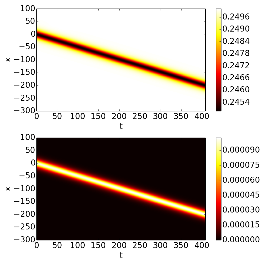
Figure 1: The solution (21)-(22) is propagated according to Eqs. (5)-(6) for the values $\epsilon=0.005$ and $\mu=Q_{0}=1$, $u_{0}=-C=0.5$. In the top and bottom panels shown are contour plots of the densities $|u(x,t)|^{2}$ and $|v(x,t)|^{2}$, respectively. The traveling DB soliton can be clearly discerned with no visible radiation in this example. The speed of the center of mass roughly agrees with the theoretical prediction of $|C|$ in this case.

In order to examine the robustness of the identified wave structures in the previous section, we now turn to direct numerical simulations. Firstly, we initialize the solution at $t=0$ according to Eqs. (21)-(22); that is, we set $u(x,0)=u^{(\epsilon)}(x,0)$ and $v(x,0)=v^{(\epsilon)}(x,0)$. The approximate solutions are then evolved in the propagation variable $t$ according to the dynamical equations (5)-(6) for the values $\mu=Q_{0}=1$. Values of $\epsilon>0$ are taken to be small and positive, in line with the main premise of the multiscale perturbation theory.

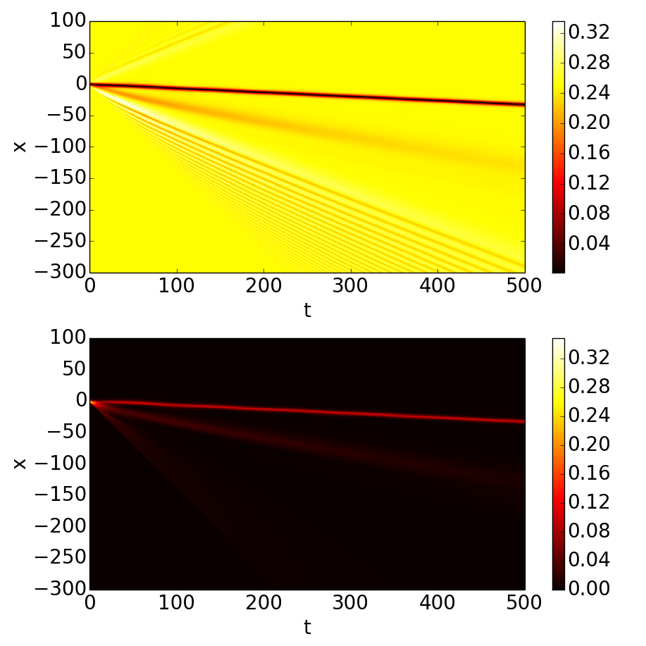
Figure 2: Similar to Fig. 1, but for $\epsilon=0.295$. Here, the theory is away from the range of its validity, yet it still distills a clear dark-bright traveling soliton. Additionally, radiation in the form of dispersive shock waves is observed to emerge in both directions traveling faster than the soliton.

As may be natural to expect, we find that for larger values of $\epsilon$ the solitons emit larger amounts of radiation. In Fig. 1, for $\epsilon=0.005$, there is essentially no visible radiation during the propagation. As we increase the value of $\epsilon$, we notice that for the larger value of $\epsilon=0.295$, the plots in Fig. 2 feature emission of radiation in both the dark and bright soliton components. This aspect is, however, interesting in a number of ways. On the one hand, and as concerns the present study –even under this strong perturbation– a robust, slowly traveling, DB soliton emerges from the process, as a result of the dynamical evolution. On the other hand, we observe radiation in the form of dark, or dark-bright dispersive shock waves dispshock , which have been studied considerably in single component BECs (see for an example involving experiments hoefer ), yet would be quite interesting to explore in the present-multi-component setting. The latter, however, are clearly beyond the scope of the present work.

To quantify the radiation, and assess how well the analytical approximation is functioning towards formulating the DB soliton, we form the power ratio:

$$R_{\star}(\epsilon,t)={\displaystyle\int_{x_{0}(t)}^{x_{1}(t)}|\phi^{(\epsilon)}(x,t)|^{2}dx}/{\displaystyle\int_{x_{0}(t)}^{x_{1}(t)}|\phi^{(\epsilon)}(x,0)|^{2}dx}.$$ (23)

where $R_{\star}$ has the following meaning: $R_{\star}=R_{B}$ refers either to the bright component for $\phi^{(\epsilon)}=v(x,t)$, or $R_{\star}=R_{D}$ refers to the dark component with $\phi^{(\epsilon)}=u(x,t)$. The window $[x_{0}(t),x_{1}(t)]$ remains a fixed length $L$ centered at the bright or dark soliton peak for all $t$-values as the soliton propagates according to Eqs. (5)-(6). Hence, the ratio $R_{\star}$ effectively measures the change in mass (occurring through a process of emission) realized in the vicinity of the soliton, and gives a measure of the potential “distortion” of the initial condition, as transcribed from our Mel’nikov system reconstruction.

For the bright ratio $R_{B}(\epsilon_{0},t)$ with $\epsilon_{0}$ fixed, the window length $L$ is computed at $t=0$ to be the minimal one, such that $\geq 99\%$ of the power of the initial profile is contained within the window. That is, the bright spot in the $v$-component is contained within the window. For the dark ratio $R_{D}(\epsilon_{0},t)$ with $\epsilon_{0}$ fixed, the window length $L$ is computed at $t=0$ to be the minimal one, such that $\geq 1\%$ of the power of the initial profile is contained within the window. Thus, the dark spot in the $u$ component is contained within the window too. In the top and middle plots of Fig. 3 we see that the power within these windows decreases for both the dark and bright soliton components as radiation leaks out of the window for increasing $t$. The radiation is more prominent for larger values of $\epsilon_{0}$, and it is essentially non-existent for a small enough value such as $\epsilon_{0}=0.005$. The bottom panel of Fig. 3 tracks the power ratio (23) as a function of increasing $\epsilon$ for the fixed values of $L=30$ and $t=400$. The radiation in the bright soliton component is more prominent than that in the dark component according to this measure. This may be attributed to the topological nature (and hence additional robustness) of the dark soliton.

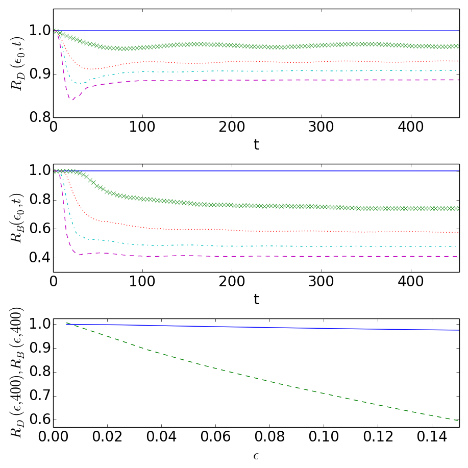
Figure 3: In the top and middle panels $R_{D}(\epsilon_{0},t)$ and $R_{B}(\epsilon_{0},t)$ are plotted as a function of $t$, for $\epsilon_{0}=0.005$ (blue solid line), $\epsilon_{0}=0.075$ (green line with x-symbols), $\epsilon_{0}=0.145$ (red dotted line), $\epsilon_{0}=0.215$ (cyan dash-dotted line), and $\epsilon_{0}=0.285$ (magenta dashed line). In the lower panel $R_{D}(\epsilon,t=400)$ (solid line) and $R_{B}(\epsilon,t=400)$ (dashed line) are plotted as a function of $\epsilon$ for $L=45$, showing that the radiation is more significant in the bright- rather than in the dark-soliton component.

III.2 DB soliton dynamics in the trap

We now consider the dynamics in the presence of a parabolic trap, namely: $V(x)=(1/2)\Omega^{2}x^{2}$, as discussed in Sec. II. Here, the presence of the trap results in the loss of the invariance with respect to spatial translations, which suggests the consideration of the original system, in the form of Eqs. (3)-(4), for $\Omega_{R}=0$.

Before “embedding” the DB soliton into our numerical scheme, we first identify stationary solutions using an initial guess based on the Thomas-Fermi approximation stringari ; pethick for the dark soliton component, namely $u\approx e^{-i\mu_{1}t}{\rm max}\left(\sqrt{\mu_{1}-V(x)},0\right)$ (where $\mu_{1}$ is the chemical potential of the $u$-component), while the bright component is absent, i.e., $v=0$. A Newton-Raphson based continuation in $\epsilon$ then allows us to numerically converge to the desired “background” (stationary) solution

$$u=u_{TF}(x),~{}~{}~{}~{}~{}~{}v=0,$$

for the full set of equations (3)-(4) (for $\Omega_{R}=0$). Here, $u_{TF}$ is the true numerical solution to the problem, rather than the approximate analytical one. Now, embedding within this background, our approximate analytical solution of Eqs. (21)-(22) from the multiscale expansion argument of Section II, gives the approximate dark-bright soliton solutions

$$u=u^{(\epsilon)}u_{TF},~{}~{}~{}~{}~{}~{}v=v^{(\epsilon)},$$

in the presence of the trap $V(x)$.

These dark-bright soliton structures oscillate over time within the trapped condensate. A typical example of the resulting oscillation is shown in Fig. 4. Here, it should be noted that we find that there are rather small-amplitude wavepackets that escape from the core of the “imprinted” waveform and reach the boundary of the domain, subsequently becoming back-scattered. To avoid such a spurious effect, over the course of the admittedly long oscillation periods of the DB soliton, we include in the numerical simulations an absorbing layer that is activated outside the region of the background solution width. This layer absorbs excess radiation in order to minimize interference with the DB soliton structure upon potential back-scatter.

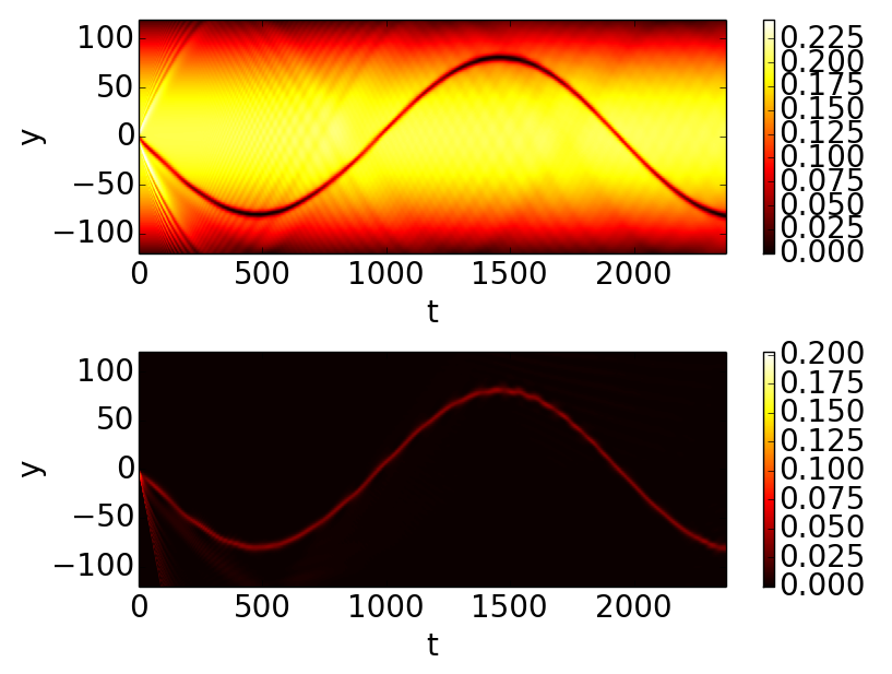
Figure 4: Density contour plot showing the oscillation of a DB soliton in a parabolic trap according to Eqs. (3)-(4) (for $\Omega_{R}=0$), for parameter values $\epsilon=0.1$, $\Omega=0.005$, $Q_{0}=4.5$, $u_{0}=1$, $\mu=\sqrt{2}$, and $\mu_{1}=0.2$.

The oscillation frequency $\omega$ of the dark-bright solitary wave is tracked as a function of the atom number of the bright soliton component,

$$N_{b}=\displaystyle\int_{x_{0}(t)}^{x_{1}(t)}|v|^{2}dx,$$ (24)

where $[x_{0}(t),x_{1}(t)]$ is a moving window centered at the bright soliton. The resulting normalized (to the trap frequency) oscillation frequency $\omega/\Omega$ is compared in Fig. 5 to the prediction of Busch and Anglin BA , for a regular (two-component) dark-bright soliton in the absence of spin-orbit coupling:

$${\omega}=\Omega\left(\frac{1}{\sqrt{2}}-\frac{N_{b}}{8\sqrt{\mu+(\frac{N_{b}}{4})^{2}}}\right).$$ (25)

Interestingly, it is found that the theoretical prediction of Eq. (25) not only provides a fair approximation to the frequency of oscillation, but, in fact, one that is progressively more accurate for higher values of $\epsilon$.

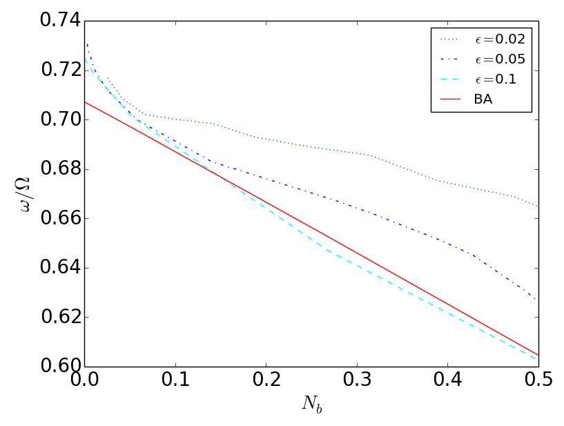
Figure 5: Normalized oscillation frequency $\omega/\Omega$ as a function of $N_{b}$ for various $\epsilon$ values. The prediction of Ref. BA [cf. Eq. (25)] is plotted as the red dashed line.

IV Discussion and Conclusions

In the present work, we have explored the possibility of the intensely studied spin-orbit (SO) coupled BECs to bear structures that are prototypical in pseudo-spinor condensates, namely dark-bright (DB) solitons. In fact, we have studied a “reduced spin-orbit coupled system”, corresponding to the absence of the linear Raman coupling (whose feasibility is worth further experimental consideration) between components. The reason for this assumption was that the presence of such a linear coupling results in the onset of population exchange between components, which makes impossible the formation of states with different boundary conditions (this was also confirmed in our simulations –results were not shown here). The studied model, apart from SO-coupled BECs, finds also applications in nonlinear optics, describing the interaction between two electric field envelopes of different frequencies in a dispersive nonlinear medium.

In this limit of zero Raman coupling, we have been able to provide a systematic perturbative method for the construction of dark-bright solitons. This method relies on the asymptotic reduction of the nonintegrable reduced SO system to the completely integrable Mel’nikov system. For the latter, exact analytical soliton solutions do exist, and can be used to reconstruct DB solitons for the reduced SO system.

The validity of our analytical approximations, and the robustness of the DB solitons, were explored via numerical computations. It was found that the solitons persist not only in the limit of sufficiently small value of the perturbation parameter $\epsilon$ (where the accuracy of the perturbation theory and the control of the associated error guarantees its relevance), but also even in the case where $\epsilon$ is not that small. Finally, we investigated the DB soliton dynamics in the more realistic setting where a parabolic trap is present. It was found that DB solitons oscillate in the trap with a frequency proximal to that predicted for “regular” DB solitons in the absence of the SO coupling.

This study opens numerous veins for future research. On the one hand, it is worthwhile to further explore the dynamics of DB solitons from the point of view of, e.g., their complex interaction dynamics (see for some recent examples, the work of lia ), and how the presence of the spin-orbit coupling could modify that. On the other hand, one could envision generalizations of the relevant structures, in the presence of spin-orbit coupling, to higher dimensions. These include the study of baby-Skyrmions –otherwise known as filled-core vortices or vortex-bright solitons– in two spatial dimensions cooper ; skryabin ; kody (see recent relevant work in Ref. ad ), and even to true skyrmions in three spatial dimensions ruost .

References

- (1) L. P. Pitaevskii and S. Stringari, Bose-Einstein Condensation (Oxford University Press, Oxford, 2003).
- (2) C. J. Pethick and H. Smith, Bose-Einstein condensation in dilute gases (Cambridge University Press, Cambridge, 2002).
- (3) P. G. Kevrekidis, D. J. Frantzeskakis, and R. Carretero-González (eds), Emergent Nonlinear Phenomena in Bose–Einstein Condensates: Theory and Experiment (Springer, Heidelberg, 2008).
- (4) P. G. Kevrekidis, D. J. Frantzeskakis, and R. Carretero-González, The Defocusing Nonlinear Schrödinger Equation. (SIAM, Philadelphia, 2015).
- (5) N. Proukakis, S. Gardiner, M. Davis, M. Szymánska (Eds.), Quantum gases: Finite temperature and nonequilibrium dynamics (Imperial College Press, London, 2013).
- (6) L. D. Carr, Understanding quantum phase transitions, (Taylor & Francis, Boca Raton, 2010).
- (7) See, e.g., the special volume: Rom. Rep. Phys. 67, 1 (2015), and more specifically the review: V. S. Bagnato, D. J. Frantzeskakis, P. G. Kevrekidis, B. A. Malomed, and D. Mihalache, Rom. Rep. Phys. 67, 5 (2015) therein.
- (8) Y.-J. Lin, K. Jimenez-Garcia, and I. B. Spielman, Nature, 471, 83 (2011).
- (9) J.-Y. Zhang, S.-C. Ji, Z. Chen, L. Zhang, Z.-D. Du, B. Yan, G.-S. Pan, B. Zhao, Y.-J. Deng, H. Zhai, S. Chen, J.-W. Pan, Phys. Rev. Lett. 109, 115301 (2012).
- (10) T. L. Ho and S. Zhang, Phys. Rev. Lett. 107, 150403 (2011); S. Sinha, R. Nath, and L. Santos, Phys. Rev. Lett. 107, 270401 (2011); Y. Li, L. P. Pitaevskii, and S. Stringari, Phys. Rev. Lett. 108, 225301 (2012).
- (11) P. Wang, Z.-Q. Yu, Z. Fu, J. Miao, L. Huang, S. Chai, H. Zhai, J. Zhang, Phys. Rev. Lett. 109, 095301 (2012).
- (12) L. W. Cheuk, A. T. Sommer, Z. Hadzibabic, T. Yefsah, W. S. Bakr, and M. W. Zwierlein, Phys. Rev. Lett. 109, 095302 (2012).
- (13) C. Qu, C. Hamner, M. Gong, C. Zhang and P. Engels, Phys. Rev. A 88, 021604(R) (2013).
- (14) L. J. LeBlanc, M. C. Beeler, K Jimenez-Garcia, A. R. Perry, S. Sugawa, R. A. Williams and I. B. Spielman, New J. Phys. 15 073011 (2013).
- (15) C. Hamner, C. Qu, Yongping Zhang, J. Chang, M. Gong, C. Zhang, P. Engels, Nature Communications 5, 4023 (2014).
- (16) M. A. Khamehchi, K. Hossain, M. E. Mossman, Yongping Zhang, Th. Busch, M. McNeil Forbes, and P. Engels, Phys. Rev. Lett. 118, 155301 (2017).
- (17) F. Gerbier, G. Juzeliünas, and P. Öhberg, Rev. Mod. Phys. 83, 1523 (2011).
- (18) V. Galitski, and I. B. Spielman, Nature, 494, 54 (2013).
- (19) N. Goldman, G. Juzeliunas, P. Ohberg, I. B. Spielman, Rep. Progr. Phys., 77, 126401 (2014).
- (20) Y. Zhang, M. E. Mossman, Th. Busch, P. Engels, C. Zhang, Front. Phys. 11, 118103 (2016).
- (21) P. G. Kevrekidis, D. J. Frantzeskakis, Rev. Phys. 1, 140 (2016).
- (22) C. Becker, S. Stellmer, P. Soltan-Panahi, S. Dörscher, M. Baumert, E.-M. Richter, J. Kronjäger, K. Bongs, and K. Sengstock, Nature Phys. 4, 496 (2008).
- (23) C. Hamner, J. J. Chang, P. Engels, and M.A. Hoefer, Phys. Rev. Lett. 106, 065302 (2011).
- (24) S. Middelkamp, J. J. Chang, C. Hamner, R. Carretero-González, P. G. Kevrekidis, V. Achilleos, D. J. Frantzeskakis, P. Schmelcher, and P. Engels, Phys. Lett. A 375, 642 (2011).
- (25) D. Yan, J. J. Chang, C. Hamner, P. G. Kevrekidis, P. Engels, V. Achilleos, D. J. Frantzeskakis, R. Carretero-González, and P. Schmelcher, Phys. Rev. A 84, 053630 (2011).
- (26) A. Álvarez, J. Cuevas, F. R. Romero, C. Hamner, J. J. Chang, P. Engels, P. G. Kevrekidis, and D. J. Frantzeskakis, J. Phys. B: At. Mol. Opt. Phys. 46, 065302 (2013).
- (27) M. A. Hoefer, J. J. Chang, C. Hamner, and P. Engels, Phys. Rev. A 84, 041605(R) (2011).
- (28) D. Yan, J. J. Chang, C. Hamner, M. Hoefer, P. G. Kevrekidis, P. Engels, V. Achilleos, D. J. Frantzeskakis, and J. Cuevas, J. Phys. B: At. Mol. Opt. Phys. 45, 115301 (2012).
- (29) I. Danaila, M. A. Khamehchi, V. Gokhroo, P. Engels, and P. G. Kevrekidis, Phys. Rev. A 94, 053617 (2016).
- (30) M. J. Ablowitz and H. Segur, Solitons and the Inverse Scattering Transform (SIAM, Philadelphia, 1981).
- (31) Z. Chen, M. Segev, T. H. Coskun, D. N. Christodoulides, and Yu.S. Kivshar, J. Opt. Soc. Am. B 14, 3066 (1997).
- (32) E. A. Ostrovskaya, Yu. S. Kivshar, Z. Chen, and M. Segev, Opt. Lett. 24, 327 (1999).
- (33) T. M. Bersano, V. Gokhroo, M. A. Khamehchi, J. D’Ambroise, D. J. Frantzeskakis, P. Engels, and P. G. Kevrekidis, arXiv:1705.08130.
- (34) H. E. Nistazakis, D. J. Frantzeskakis, P. G. Kevrekidis, B. A. Malomed, and R. Carretero-González, Phys. Rev. A 77, 033612 (2008).
- (35) V. Achilleos, D. J. Frantzeskakis, P. G. Kevrekidis, and D. E. Pelinovsky, Phys. Rev. Lett. 110, 264101 (2013).
- (36) Yong Xu, Yongping Zhang, and Biao Wu, Phys. Rev. A 87, 013614 (2013).
- (37) V. Achilleos, J. Stockhofe, P. G. Kevrekidis, D. J. Frantzeskakis, and P. Schmelcher, Europhys. Lett. 103, 20002 (2013).
- (38) V. Achilleos, D. J. Frantzeskakis, and P. G. Kevrekidis, Phys. Rev. A 89, 033636 (2014).
- (39) Y. V. Kartashov, V. V. Konotop and F. Kh. Abdullaev, Phys. Rev. Lett. 111, 060402 (2013).
- (40) V. E. Lobanov, Y. V. Kartashov, and V. V. Konotop, Phys. Rev. Lett. 112, 180403 (2014).
- (41) Yongping Zhang, Yong Xu, and Th. Busch, Phys. Rev. A 91, 043629 (2015).
- (42) Lin Wen, Q. Sun, Yu Chen, Deng-Shan Wang, J. Hu, H. Chen, W.-M. Liu, G. Juzeliūnas, B. A. Malomed, and An-Chun Ji, Phys. Rev. A 94, 061602(R) (2016).
- (43) V. Achilleos, D. J. Frantzeskakis, P. G. Kevrekidis, P. Schmelcher, and J. Stockhofe, Rom. Rep. Phys. 67, 235 (2015).
- (44) Y. V. Kartashov, V. V. Konotop, and D. A. Zezyulin, Phys. Rev. A 90, 063621 (2014).
- (45) Y. V. Kartashov and V. V. Konotop, Phys. Rev. Lett. 118, 190401 (2017).
- (46) H. Sakaguchi, B. Li, and B. A. Malomed, Phys. Rev. E 89, 032920 (2014).
- (47) Y.-C. Zhang, Z.-W. Zhou, B. A. Malomed, and H. Pu, Phys. Rev. Lett. 115, 253902 (2015).
- (48) H. Sakaguchi, E. Ya. Sherman, and B. A. Malomed, Phys. Rev. E 94, 032202 (2016).
- (49) Xunda Jiang, Zhiwei Fan, Zhaopin Chen, Wei Pang, Yongyao Li, and B. A. Malomed, Phys. Rev. A 93, 023633 (2016).
- (50) Yongyao Li, Yan Liu, Zhiwei Fan, Wei Pang, Shenhe Fu, and B. A. Malomed, Phys. Rev. A 95, 063613 (2017).
- (51) D. Mihalache, Rom. Rep. Phys. 69, 403 (2017).
- (52) P. Villain and M. Lewenstein, Phys. Rev. A 59, 2250 (1999); J. Williams, R. Walser, J. Cooper, E. A. Cornell, and M. Holland, Phys. Rev. A 61, 033612 (2000); A. Smerzi, A. Trombettoni, T. Lopez-Arias, C. Fort, P. Maddaloni, F. Minardi, and M. Inguscio, Eur. Phys. J. B 31, 457 (2003); B. Deconinck, P. G. Kevrekidis, H. E. Nistazakis, and D. J. Frantzeskakis, Phys. Rev. A 70, 063605 (2004).
- (53) Yu. S. Kivshar and G. P. Agrawal, Optical solitons: from fibers to photonic crystals, Academic Press (San Diego, 2003).
- (54) N. M. Ryskin, JETP 79, 833 (1994).
- (55) Yu. S. Kivshar and D. E. Pelinovsky, Phys. Rep. 331, 117, (2000).
- (56) R. Carretero-González, D. J. Frantzeskakis, and P. G. Kevrekidis, Nonlinearity 21, R139 (2008).
- (57) D. J. Frantzeskakis, J. Phys. A: Math. Theor. 43, 213001 (2010).
- (58) V. K. Mel’nikov, Lett. Math. Phys. 7, 129 (1983).
- (59) V. K. Mel’nikov, Phys. Let. A 128, 488 (1988).
- (60) Y. A. Bychkov and E. I. Rashba, J. Phys. C 17, 6039 (1984).
- (61) G. Dresselhaus, Phys. Rev. 100, 580 (1955).
- (62) D. J. Frantzeskakis, Phys. Lett. A 285, 363 (2001).
- (63) M. Aguero, D. J. Frantzeskakis, and P. G. Kevrekidis, J. Phys. A: Math. Gen. 39, 7705 (2006).
- (64) F. Tsitoura, V. Achilleos, B. A. Malomed, D. Yan, P. G. Kevrekidis, and D. J. Frantzeskakis, Phys. Rev. A 87, 063624 (2013).
- (65) T. P. Horikis and D. J. Frantzeskakis, Phys. Rev. A 94, 053805 (2016).
- (66) V. K. Mel’nikov, Phys. Lett. A 133, 493 (1988).
- (67) See, e.g., M. Hoefer, M. Ablowitz, Dispersive Schock Waves, Scholarpedia, and the recent review: G. A. El and M. A. Hoefer, Physica D 333, 11 (2016).
- (68) M. A. Hoefer, M. J. Ablowitz, I. Coddington, E. A. Cornell, P. Engels, and V. Schweikhard Phys. Rev. A 74, 023623 (2006).
- (69) Th. Busch and J. R. Anglin, Phys. Rev. Lett. 87, 010401 (2001)
- (70) G. C. Katsimiga, J. Stockhofe, P. G. Kevrekidis, and P. Schmelcher, Phys. Rev. A 95, 013621 (2017); G. C. Katsimiga, J. Stockhofe, P. G. Kevrekidis, and P. Schmelcher, Appl. Sci. 7, 388 (2017).
- (71) R. A. Battye, N. R. Cooper, and P. M. Sutcliffe, Phys. Rev. Lett. 88, 080401 (2002).
- (72) D. V. Skryabin, Phys. Rev. A 63, 013602 (2001).
- (73) K. J. H. Law, P. G. Kevrekidis, and L. S. Tuckerman, Phys. Rev. Lett. 105, 160405 (2010).
- (74) S. Gautam and S. K. Adhikari, Phys. Rev. A 95, 013608 (2017).
- (75) J. Ruostekoski and J. R. Anglin Phys. Rev. Lett. 86, 3934 (2001); C. M. Savage and J. Ruostekoski Phys. Rev. Lett. 91, 010403 (2003).