Function space analysis of deep learning representation layers

Abstract

In this paper we propose a function space approach to Representation Learning [3] and the analysis of the representation layers in deep learning architectures. We show how to compute a ‘weak-type’ Besov smoothness index that quantifies the geometry of the clustering in the feature space. This approach was already applied successfully to improve the performance of machine learning algorithms such as the Random Forest [22] and tree-based Gradient Boosting [14]. Our experiments demonstrate that in well-known and well-performing trained networks, the Besov smoothness of the training set, measured in the corresponding hidden layer feature map representation, increases from layer to layer. We also contribute to the understanding of generalization [49] by showing how the Besov smoothness of the representations, decreases as we add more mis-labeling to the training data. We hope this approach will contribute to the de-mystification of some aspects of deep learning.

1 Introduction

An excellent starting point for this paper is the survey on Representation Learning [3]. One of the main issues raised in this survey is that simple smoothness assumptions on the data do not hold. That is, there exists a curse of dimensionality and ‘close’ feature representations do not map to ‘similar’ values. The authors write: “We advocate learning algorithms that are flexible and non-parametric but do not rely exclusively on the smoothness assumption”.

In this work we do in fact advocate smoothness analysis of representation layers, yet in line with [3], our notion of smoothness is indeed flexible, adaptive and non-parametric. We rely on geometric multivariate function space theory and use a machinery of Besov ‘weak-type’ smoothness which is robust enough to support quantifying smoothness of high dimensional discontinuous functions.

Although machine learning is mostly associated with the field of statistics we argue that the popular machine learning algorithms such as Support Vector Machines, Tree-Based Gradient Boosting and Random Forest (see e.g [28]), are in fact closely related to the field of multivariate adaptive approximation theory. In essence, these algorithms work best if there exists geometric structure of clusters in the feature space. If such geometry exists, these algorithms will capture it, by segmenting out the different clusters. We claim that in the absence of such geometry, these machine learning algorithms will fail.

However, this is exactly where Deep Learning (DL) comes into play. In the absence of a geometrical structure in the given initial representation space, the goal of the DL layers is to create a series of transformations from one representation space to the next, where structure of the geometry of the clusters improves sequentially. We quote [10]: “The whole process of applying this complex geometric transformation to the input data can be visualized in 3D by imagining a person trying to uncrumple a paper ball: the crumpled paper ball is the manifold of the input data that the model starts with. Each movement operated by the person on the paper ball is similar to a simple geometric transformation operated by one layer. The full uncrumpling gesture sequence is the complex transformation of the entire model. Deep learning models are mathematical machines for uncrumpling complicated manifolds of high-dimensional data”.

Let us provide an instructive example: Assume we are presented with a set of gray-scale images of dimension $\sqrt{n_{0}}\times\sqrt{n_{0}}$ with $L$ class labels. Assume further that a DL network has been successfully trained to classify these images with relatively high precision. This allows us to extract the representation of each image in each of the hidden layers. To create a representation at layer $0$, we concatenate the $\sqrt{n_{0}}$ rows of pixel values of each image, to create a vector of dimension $n_{0}$. We also normalize the pixel values to the range $[0,1]$. Since we advocate a function-theoretical approach, we transform the class labels into vector-values in the space ${\mathbb{R}}^{L-1}$ by assigning each label to a vertex of a standard simplex (see Section 2 below). Thus, the images are considered as samples of a function $f_{0}:[0,1]^{n_{0}}\rightarrow{\mathbb{R}}^{L-1}$. In the general case, there is no hope that there exists geometric clustering of the classes in this initial feature space and that $f_{0}$ has sufficient ‘weak-type’ smoothness (as is verified by our experiments below). Thus, a transform into a different feature space is needed. We thus associate with each $k$-th layer of a DL network, a function $f_{k}:[0,1]^{n_{k}}\rightarrow{\mathbb{R}}^{L-1}$ where the samples are vectors created by normalizing and concatenating the feature maps computed from each of the images. Interestingly enough, although the series of functions $f_{k}$ are embedded in different dimensions $n_{k}$, through the simple normalizing of the features, our method is able to assign smoothness indices to each layer that are comparable. We claim that for well performing networks, the representations in general ‘improve’ from layer to layer and that our method captures this phenomena and shows the increase of smooothness.

Related work is [38] where an architecture of Convolutional Sparse Coding was analyzed. The connection to this work is the emphasis on ‘sparsity’ analysis of hidden layers. However, there are significant differences since we advocate a function space theoretical analysis of any neural network architecture in current use. Also, there is the recent work [42], where the authors take an ‘information-theoretical’ approach to the analysis of the stochastic gradient descent optimization of DL networks and the representation layers. One can safely say that all of the approaches, including the one presented here, need to be further evaluated on larger datasets and deeper architectures.

The paper is organized as follows: In Section 2 we review our smoothness analysis machinery which is the Wavelet Decomposition of Random Forest (RF) [22]. In Section 3 we present the required geometric function space theoretical background. Since we are comparing different representations over different spaces of different dimensions, we add to the theory presented in [22] relevant ‘dimension-free’ results. In Section 4 we show how to apply the theory in practice. Specifically, how the wavelet decomposition of a RF can be used to numerically compute a Besov ‘weak-type’ smoothness index of a given function in any representation space (e.g hidden layer). Section 5 provides experimental results that demonstrate how our theory is able to explain empirical findings in various scenarios. Finally, Section 6 presents our conclusions as well as future work.

2 Wavelet decomposition of Random Forests

To measure smoothness of a dataset at the various DL representation layers, we apply the construction of wavelet decompositions of Random Forests [22]. Wavelets [13], [34] and geometric wavelets [15], [1], are a powerful yet simple tool for constructing sparse representations of ‘complex’ functions. The Random Forest (RF) [4], [11], [28] introduced by Breiman [5], [6], is a very effective machine learning method that can be considered as a way to overcome the ‘greedy’ nature and high variance of a single decision tree. When combined, the wavelet decomposition of the RF unravels the sparsity of the underlying function and establishes an order of the RF nodes from ‘important’ components to ‘negligible’ noise. Therefore, the method provides a better understanding of any constructed RF. Furthermore, the method is a basis for a robust feature importance algorithm. We note that one can apply a similar approach to improve the performance of tree-based Gradient Boosting algorithms [14].

We begin with an overview of single trees. In statistics and machine learning [7], [2], [4], [16], [28] the construction is called a Decision Tree or the Classification and Regression Tree (CART). We are given a real-valued function $f\in L_{2}\left({\Omega_{0}}\right)$ or a discrete dataset $\left\{{x_{i}\in\Omega_{0},f\left({x_{i}}\right)}\right\}_{i\in I}$, in some convex bounded domain $\Omega_{0}\subset{\mathbb{R}}^{n}$. The goal is to find an efficient representation of the underlying function, overcoming the complexity, geometry and possibly non-smooth nature of the function values. To this end, we subdivide the initial domain $\Omega_{0}$ into two subdomains, e.g. by intersecting it with a hyper-plane. The subdivision is performed to minimize a given cost function. This subdivision process then continues recursively on the subdomains until some stopping criterion is met, which in turn, determines the leaves of the tree. We now describe one instance of the cost function which is related to minimizing variance. At each stage of the subdivision process, at a certain node of the tree, the algorithm finds, for the convex domain $\Omega\subset{{\mathbb{R}}}^{n}$ associated with the node:

(i) A partition by an hyper-plane into two convex subdomains ${\Omega}^{\prime},{\Omega}^{\prime\prime}$, $\Omega^{\prime}\cup{\Omega}^{\prime\prime}=\Omega$,

(ii) Two multivariate polynomials $Q_{{\Omega}^{\prime}},Q_{{\Omega}^{\prime\prime}}\in\Pi_{r-1}\left({{\mathbb{R}}^{n}}\right)$, of fixed (typically low) total degree r $-$ 1.

The partition and the polynomials are chosen to minimize the following quantity

$$\left\|{f-Q_{\Omega^{\prime}}}\right\|_{L_{p}\left({{\Omega}^{\prime}}\right)}^{p}+\left\|{f-Q_{\Omega^{\prime\prime}}}\right\|_{L_{p}\left({{\Omega}^{\prime\prime}}\right)}^{p}.$$ (2.1)

Here, for $1\leq p<\infty$, we used the definition

$$\left\|g\right\|_{L_{p}\left({\tilde{{\Omega}}}\right)}:=\left({\int_{\tilde{{\Omega}}}{\left|{g\left(x\right)}\right|^{p}dx}}\right)^{1/p}.$$

If the dataset is discrete, consisting of feature vectors $x_{i}\in{\mathbb{R}}^{n},i\in I$ , with response values $f\left({x_{i}}\right)$, then a discrete functional is minimized over all partitions $\Omega^{\prime}\cup{\Omega}^{\prime\prime}=\Omega$

$$\sum\limits_{x_{i}\in{\Omega}^{\prime}}{\left|{f\left({x_{i}}\right)-Q_{{\Omega}^{\prime}}(x_{i})}\right|^{p}}+\sum\limits_{x_{i}\in{\Omega}^{\prime\prime}}{\left|{f\left({x_{i}}\right)-Q_{{\Omega}^{\prime\prime}}(x_{i})}\right|^{p}}.$$ (2.2)

Observe that for any given subdividing hyperplane, the approximating polynomials in (2.2) can be uniquely determined for $p=2$, by least square minimization. For the order $r=1$, the approximating polynomials are nothing but the mean of the function values over each of the subdomains

$$Q_{{\Omega}^{\prime}}\left(x\right)=C_{{\Omega}^{\prime}}=\frac{1}{\#\left\{{x_{i}\in{\Omega}^{\prime}}\right\}}\sum\limits_{x_{i}\in{\Omega}^{\prime}}{f\left({x_{i}}\right)},$$

$$Q_{{\Omega}^{\prime\prime}}\left(x\right)=C_{{\Omega}^{\prime\prime}}=\frac{1}{\#\left\{{x_{i}\in{\Omega}^{\prime\prime}}\right\}}\sum\limits_{x_{i}\in{\Omega}^{\prime\prime}}{f\left({x_{i}}\right)}.$$

In many applications of decision trees, the high-dimensionality of the data does not allow to search through all possible subdivisions. As in our experimental results, one may restrict the subdivisions to the class of hyperplanes aligned with the main axes. In contrast, there are cases where one would like to consider more advanced form of subdivisions, where they take certain hyper-surface form or even non-linear forms through kernel Support Vector Machines. Our paradigm of wavelet decompositions can support in principle all of these forms.

Random Forest (RF) is a popular machine learning tool that collects decision trees into an ensemble model [5],[4]. The trees are constructed independently in a diverse fashion and prediction is done by a voting mechanism among all trees. A key element [5], is that large diversity between the trees reduces the ensemble’s variance. There are many RFs variations that differ in the way randomness is injected into the model, e.g bagging, random feature subset selection and the partition criterion [11], [28]. Our wavelet decomposition paradigm is applicable to most of the RF versions known from the literature.

Bagging [6] is a method that produces partial replicates of the training data for each tree. A typical approach is to randomly select for each tree a certain percentage of the training set (e.g. 80%) or to randomly select samples with repetitions [28].

Additional methods to inject randomness can be achieved at the node partitioning level. For each node, we may restrict the partition criteria to a small random subset of the parameter values (hyper-parameter). A typical selection is to search for a partition from a random subset of $\sqrt{n}$  features [5]. This technique is also useful for reducing the amount of computations when searching the appropriate partition for each node. Bagging and random feature selections are not mutually exclusive and could be used together.

For $j=1,...,J$, one creates a decision tree ${\cal T}_{j}$, based on a subset of the data, $X^{j}$. One then provides a weight (score) $w_{j}$ to the tree ${\cal T}_{j}$, based on the estimated performance of the tree, where $\sum_{j=1}^{J}{w_{j}}=1$. In the supervised learning, one typically uses the remaining data points $x_{i}\notin X^{j}$ to evaluate the performance of ${\cal T}_{j}$. For simplicity, we will mostly consider in this paper the choice of uniform weights $w_{j}=1/J$. For any point $x\in\Omega_{0}$, the approximation associated with the $j^{th}$ tree, denoted by $\tilde{{f}}_{j}\left({x}\right)$, is computed by finding the leaf $\Omega\in{\cal T}_{j}$ in which $x$ is contained and then evaluating $\tilde{{f}}_{j}\left({x_{i}}\right):=Q_{\Omega}\left({x}\right)$, where $Q_{\Omega}$ is the corresponding polynomial associated with the decision node $\Omega$. One then assigns an approximate value to any point $x\in\Omega_{0}$ by

$$\tilde{{f}}\left(x\right)=\sum\limits_{j=1}^{J}{w_{j}\tilde{{f}}_{j}\left(x\right)}.$$

Typically, in classification problems, the response variable does have a numeric value, but is labeled by one of L classes. In this scenario, each input training point $x_{i}\in\Omega_{0}$ is assigned with a class $Cl\left({x_{i}}\right)$. To convert the problem to the ‘functional’ setting described above one assigns to each class the value of a node on the regular simplex consisting of $L$ vertices in ${{\mathbb{R}}}^{L-1}$ (all with equal pairwise distances). Thus, we may assume that the input data is in the form

$$\left\{{x_{i},Cl\left({x_{i}}\right)}\right\}_{i\in I}\in\left({{\mathbb{R}}^{n},{{\mathbb{R}}}^{L-1}}\right).$$

In this case, if we choose approximation using constants ($r=1)$, then the calculated mean over any subdomain $\Omega$ is in fact a point $\vec{{E}}_{\Omega}\in{{\mathbb{R}}}^{L-1}$, inside the simplex. Obviously, any value inside the multidimensional simplex, can be mapped back to a class, along with an estimated confidence level, by calculating the closest vertex of the simplex to it.

Following the classic paradigm of nonlinear approximation using wavelets [13],[17],[34] and the geometric function space theory presented in [15], [30], we introduced in [22] a construction of a wavelet decomposition of a forest. Let ${\Omega}^{\prime}$ be a child of $\Omega$ in a tree ${\cal T}$, i.e. ${\Omega}^{\prime}\subset\Omega$ and ${\Omega}^{\prime}$ was created by a partition of $\Omega$. Denote by ${\rm{\bf 1}}_{{\Omega}^{\prime}}$, the indicator function over the child domain ${\Omega}^{\prime}$, i.e. ${\rm{\bf 1}}_{{\Omega}^{\prime}}\left(x\right)=1$, if $x\in{\Omega}^{\prime}$ and ${\rm{\bf 1}}_{{\Omega}^{\prime}}\left(x\right)=0$, if $x\notin{\Omega}^{\prime}$. We use the polynomial approximations $Q_{{\Omega}^{\prime}},Q_{\Omega}\in\Pi_{r-1}\left({{{\mathbb{R}}}^{n}}\right)$, computed by the local minimization (2.1) and define

$$\psi_{{\Omega}^{\prime}}(x):=\psi_{{\Omega}^{\prime}}\left(f\right)(x):={\rm{\bf 1}}_{{\Omega}^{\prime}}(x)\left({Q_{{\Omega}^{\prime}}(x)-Q_{\Omega}}(x)\right),$$ (2.3)

as the geometric wavelet associated with the subdomain ${\Omega}^{\prime}$ and the function $f$, or the given discrete dataset $\left\{{x_{i},f\left({x_{i}}\right)}\right\}_{i\in I}$. Each wavelet $\psi_{{\Omega}^{\prime}}$, is a ‘local difference’ component that belongs to the detail space between two levels in the tree, a ‘low resolution’ level associated with $\Omega$ and a ‘high resolution’ level associated with ${\Omega}^{\prime}$. Also, the wavelets (2.3) have the ‘zero moments’ property, i.e., if the response variable is sampled from a polynomial of degree $r-1$ over $\Omega$, then our local scheme will compute $Q_{{\Omega}^{\prime}}\left(x\right)=Q_{\Omega}\left(x\right)=f\left(x\right)$, $\forall x\in\Omega$, and therefore $\psi_{{\Omega}^{\prime}}=0$.

Under certain mild conditions on the tree ${\cal T}$ and the function $f$, we have by the nature of the wavelets, the ‘telescopic’ sum of differences

$$f=\sum\limits_{\Omega\in{\cal T}}{\psi_{\Omega}},\qquad\psi_{\Omega_{0}}:=Q_{\Omega_{0}}.$$ (2.4)

For example, (2.4) holds in $L_{p}$-sense, $1\leq p<\infty$, if $f\in L_{p}\left({\Omega_{0}}\right)$ and for any $x\in\Omega_{0}$ and series of domains $\Omega_{l}\in{\cal T}$, each on a level $l$, with $x\in\Omega_{l}$ , we have that $\lim\limits_{l\to\infty}\mbox{diam}\left({\Omega_{l}}\right)=0$.

The norm of a wavelet is computed by

$$\left\|{\psi_{{\Omega}^{\prime}}}\right\|_{p}^{p}=\int_{{\Omega}^{\prime}}{\left({Q_{{\Omega}^{\prime}}\left(x\right)-Q_{\Omega}\left(x\right)}\right)^{p}dx}.$$

For the case $r=1$, where $Q_{{\Omega}}\left(x\right)=C_{\Omega}$ and $Q_{{\Omega}^{\prime}}\left(x\right)=C_{\Omega^{\prime}}$ this simplifies to

$$\left\|{\psi_{{\Omega}^{\prime}}}\right\|_{p}^{p}=\left|{{C}_{{\Omega}^{\prime}}-C_{\Omega}}\right|^{p}\left|\Omega^{\prime}\right|,$$ (2.5)

where $\left|\Omega^{\prime}\right|$ denotes the volume of $\Omega^{\prime}$. Observe that for $r=1$, the subdivision process for partitioning a node by minimizing (2.1) is equivalent to maximizing the sum of squared norms of the wavelets that are formed in that partition (see [22]).

Recall that our approach is to convert classification problems into a ‘functional’ setting by assigning the $L$ class labels to vertices of a simplex in ${\mathbb{R}}^{L-1}$. In such cases of multi-valued functions, choosing $r=1$, the wavelet $\psi_{{\Omega}^{\prime}}:{{\mathbb{R}}}^{n}\to{\mathbb{R}}^{L-1}$ is

$$\psi_{{\Omega}^{\prime}}(x)={\rm{\bf 1}}_{{\Omega}^{\prime}}(x)\left({\vec{{E}}_{{\Omega}^{\prime}}-\vec{{E}}_{\Omega}}\right),$$

and its norm is given by

$$\left\|{\psi_{{\Omega}^{\prime}}}\right\|_{p}^{p}=\left\|{\vec{{E}}_{{\Omega}^{\prime}}-\vec{{E}}_{\Omega}}\right\|_{l_{2}}^{p}\left|\Omega^{\prime}\right|,$$ (2.6)

where for $\vec{{v}}\in{{\mathbb{R}}}^{L-1}$,$\left\|{\vec{{v}}}\right\|_{l_{2}}:=\sqrt{\sum\nolimits_{i=1}^{L-1}{v_{i}^{2}}}$.

Using any given weights assigned to the trees, we obtain a wavelet representation of the entire RF

$$\tilde{{f}}\left(x\right)=\sum\limits_{j=1}^{J}{\sum\limits_{\Omega\in{\cal T}_{j}}{w_{j}\psi_{\Omega}\left(x\right)}}.$$ (2.7)

The theory (see [22]) tells us that sparse approximation is achieved by ordering the wavelet components based on their norm

$$w_{j\left({\Omega_{k_{1}}}\right)}\left\|{\psi_{\Omega_{k_{1}}}}\right\|_{p}\geq w_{j\left({\Omega_{k_{2}}}\right)}\left\|{\psi_{\Omega_{k_{3}}}}\right\|_{p}\geq\cdots$$ (2.8)

with the notation $\Omega\in{\cal T}_{j}\Rightarrow j\left(\Omega\right)=j$. Thus, the adaptive M-term approximation of a RF is

$$f_{M}\left(x\right):=\sum\limits_{m=1}^{M}{w_{j\left({\Omega_{k_{m}}}\right)}\psi_{\Omega_{k_{m}}}\left(x\right)}.$$ (2.9)

Observe that, contrary to most existing tree pruning techniques, where each tree is pruned separately, the above approximation process applies a ‘global’ pruning strategy where the significant components can come from any node of any of the trees at any level. For simplicity, one could choose $w_{j}=1\mathord{\left/{\vphantom{1J}}\right.\kern-1.2pt}J$, and obtain

$$f_{M}\left(x\right)=\frac{1}{J}\sum\limits_{m=1}^{M}{\psi_{\Omega_{k_{m}}}\left(x\right)}.$$ (2.10)

Figure 1 depicts an M-term (2.10) selected from an RF ensemble. The red colored nodes illustrate the selection of the M wavelets with the highest norm values from the entire forest. Observe that they can be selected from any tree at any level, with no connectivity restrictions.

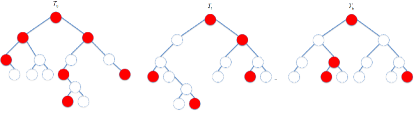
Figure 1: Selection of an M-term approximation from the entire forest.

Figure 2 depicts how the parameter $M$ is selected for the challenging “Red Wine Quality” dataset from the UCI repository [45]. The generation of 10 decision trees on the training set creates approximately 3500 wavelets. The parameter M is then selected by minimization of the approximation error on an OOB validation set. In contrast with other pruning methods [32], using (2.8), the wavelet approximation method may select significant components from any tree and any level in the forest. By this method, one does not need to predetermine the maximal depth of the trees and over-fitting is controlled by the selection of significant wavelet components.

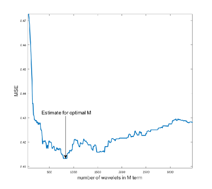
Figure 2: “Red Wine Quality” dataset - Numeric computation of M for optimal regression.

3 Geometric multivariate function space theory

An important research area of approximation theory, pioneered by Pencho Petrushev, is the characterization of adaptive geometric approximation algorithms by generalizations of the classic ‘isotropic’ Besov space to more ‘geometric’ Besov-type spaces [12], [15], [30]. We first review the definition and results of [22]. In essence, this is a generalization of a theoretical framework that has been successfully applied in the context of low dimensional and structured signal processing [17], [20]. However, in the context of machine learning, we need to analyze unstructured and possibly high dimensional datasets.

Approximation Theory relates the sparsity of a function to its Besov smoothness index and supports cases where the function is not even continuous. For a function $f\in L_{\tau}\left({\Omega}\right)$, $0<\tau\leq\infty$, $h\in{{\mathbb{R}}}^{n}$ and $r\in{{\mathbb{N}}}$, we recall the $r$-th order difference operator

$$\Delta_{h}^{r}\left({f,x}\right) := \Delta_{h}^{r}\left({f,\Omega,x}\right)$$

$$:= \sum\limits_{k=0}^{r}{\left({-1}\right)^{r+k}\left({{\begin{array}[]{*{20}c}r\hfill\\ k\hfill\\ \end{array}}}\right)f\left({x+kh}\right)},$$

where we assume the segment $\left[{x,x+rh}\right]$ is contained in $\Omega$. Otherwise, we set the $\Delta_{h}^{r}\left({f,\Omega,x}\right)=0$. The modulus of smoothness of order $r$ is defined by

$$\omega_{r}\left({f,t}\right)_{\tau}:={\sup}_{\left|h\right|\leq t}\left\|{\Delta_{h}^{r}\left({f,\Omega,\cdot}\right)}\right\|_{L_{\tau}\left(\Omega\right)},\quad t>0,$$

where for $h\in{{\mathbb{R}}}^{n}$, $\left|h\right|$ denotes the norm of $h$. We also denote

$$\omega_{r}\left({f,\Omega}\right)_{\tau}:=\omega_{r}\left({f,\frac{diam\left(\Omega\right)}{r}}\right)_{\tau}.$$ (3.2)

Next, we define the ‘weak-type’ Besov smoothness of a function, subject to the geometry of a single (possibly adaptive) tree

Definition 3.1

For $0<p<\infty$ and $\alpha>0$, we set $\tau=\tau\left({\alpha,p}\right)$, to be $1/\tau:=\alpha+1/p$. For a given function $f\in L_{p}\left({\Omega_{0}}\right)$, $\Omega_{0}\subset{{\mathbb{R}}}^{n}$, and tree ${\cal T}$, we define the associated B-space smoothness in ${\cal B}_{\tau}^{\alpha,r}\left({\cal T}\right)$, $r\in{\rm N}$, by

$$\left|f\right|_{{\cal B}_{\tau}^{\alpha,r}\left({\cal T}\right)}:=\left({\sum\limits_{\Omega\in{\cal T}}{\left({\left|\Omega\right|^{-\alpha}\omega_{r}\left({f,\Omega}\right)_{\tau}}\right)^{\tau}}}\right)^{1/\tau},$$ (3.3)

where, $\left|\Omega\right|$ denotes the volume of $\Omega$.

This notion of smoothness allows to handle functions that are not even continuous. The higher the index $\alpha$ for which (3.3) is finite, the smoother the function is. This generalizes the Sobolev smoothness of differentiable functions that have their partial derivatives integrable in some $L_{\tau}$ space. Also, the above definition generalizes the classical function space theory of Besov spaces, where the tree partitions are non-adaptive. In fact, classical Besov spaces are a special case, where the tree is constructed by partitioning into dyadic cubes, each time using $n$ levels of the tree. We recall that a ‘well clustered’ function is in fact infinitely smooth in the right adaptively chosen Besov space.

Lemma 3.2

Let $f\left(x\right)=\sum\limits_{k=1}^{K}{P_{k}\left(x\right){\rm{\bf 1}}_{B_{k}}\left(x\right)}$, where each $B_{k}\subset\Omega_{0}$ is a box with sides parallel to the main axes and $P_{k}\in\Pi_{r-1}$. We further assume that $B_{k}\cap B_{j}=\emptyset$, whenever $j\neq k$. Then, there exists an adaptive tree partition ${\cal T}$, such that $f\in B_{\alpha}^{\alpha,r}\left({\cal T}\right)$, for any $\alpha>0$.

Proof:

See [22]. ∎

For a given forest ${\cal F}=\left\{{{\cal T}_{j}}\right\}_{j=1}^{J}$ and weights $w_{j}=1\mathord{\left/{\vphantom{1J}}\right.\kern-1.2pt}J$, the $\alpha$- Besov semi-norm associated with the forest is

$$\left|f\right|_{{\cal B}_{\tau}^{\alpha,r}\left({\cal F}\right)}:=\frac{1}{J}\left({\sum\limits_{j=1}^{J}{\left|f\right|_{{\cal B}_{\tau}^{\alpha,r}\left({{\cal T}_{j}}\right)}^{\tau}}}\right)^{1/\tau}.$$ (3.4)

Definition 3.3

Given a (possibly adaptive) forest representation, we define the Besov smoothness index of $f$ by the maximal index $\alpha$ for which (3.4) is finite.

Remark It is known that different geometric approximation schemes are characterized by different flavors of Besov-type smoothness. In this work, for example, all of our experimental results compute smoothness of representations using partitions along the main $n$ axes. This restriction may lead, in general, to potentially lower Besov smoothness of the underlying function and lower sparsity of the wavelet representation. Yet, the theoretical definitions and results of this paper can also apply to more generalized schemes where, for example, tree partitions are performed using arbitrary hyper-planes. In such a case, the smoothness index of a given function may increase.

Next, for a given tree ${\cal T}$ and parameter $0<\tau<p$, we denote the $\tau$-sparsity of the tree by

$$N_{\tau}\left({f,{\cal T}}\right)=\left({\sum\limits_{\Omega\neq\Omega_{0},\Omega\in{\cal T}}{\left\|{\psi_{\Omega}}\right\|_{p}^{\tau}}}\right)^{1/\tau}.$$ (3.5)

Let us further denote the $\tau$-sparsity of a forest ${\cal F}$, by

$$N_{\tau}\left({f,{\cal F}}\right) :=\frac{1}{J}\left({\sum\limits_{j=1}^{J}{\sum\limits_{\Omega\neq\Omega_{0},\Omega\in{\cal T}_{j}}{\left\|{\psi_{\Omega}}\right\|_{p}^{\tau}}}}\right)^{1/\tau}$$

$$=\frac{1}{J}\left({\sum\limits_{j=1}^{J}{N_{\tau}\left({f,{\cal T}_{j}}\right)^{\tau}}}\right)^{1/\tau}.$$

In the setting of a single tree constructed to represent a real-valued function and under mild conditions on the partitions (see remark after (2.4) and condition (3.8)) , the theory of [15] proves the equivalence

$$\left|f\right|_{{\cal B}_{\tau}^{\alpha,r}\left({\cal T}\right)}\sim N_{\tau}\left({f,{\cal T}}\right).$$ (3.6)

This implies that there are constants $0<C_{1}<C_{2}<\infty$, that depend on parameters such as $\alpha,p,n,r$ and $\rho$ in condition (3.8) below, such that

$$C_{1}\left|f\right|_{{\cal B}_{\tau}^{\alpha,r}\left({\cal T}\right)}\leq N_{\tau}\left({f,{\cal T}}\right)\leq C_{2}\left|f\right|_{{\cal B}_{\tau}^{\alpha,r}\left({\cal T}\right)}.$$

Therefore, we also have for the forest model

$$\left|f\right|_{{\cal B}_{\tau}^{\alpha,r}\left({\cal F}\right)}\sim N_{\tau}\left({f,{\cal F}}\right).$$ (3.7)

In the setting in which we wish to apply our function theoretical approach, we are comparing smoothness of representation over different layers of DL networks. This implies that we are analyzing and comparing the smoothness a set of functions $f_{k}$, each over a different representation space of a different dimension $n_{k}$. This is, in some sense, non-standard in function space theory, where the space, or at least the dimension, over which the functions have their domain is typically fixed. Specifically, observe that the equivalence (3.7) depends on the dimension $n$ of the feature space. To this end, we add to the theory ‘dimension-free’ analysis for the case $r=1$.

We begin with a Jackson-type estimate for the degree of the adaptive wavelet forest approximation, which we keep ‘dimension free’ for the case $r=1$.

Theorem 3.4

Let ${\cal F}=\left\{{{\cal T}_{j}}\right\}_{j=1}^{J}$ be a forest. Assume there exists a constant $0<\rho<1$, such that for any domain $\Omega\in{\cal F}$ on a level $l$ and any domain ${\Omega}^{\prime}\in{\cal F}$, on the level $l+1$, with $\Omega\cap{\Omega}^{\prime}\neq\emptyset$, we have

$$\left|{{\Omega}^{\prime}}\right|\leq\rho\left|\Omega\right|,$$ (3.8)

where $\left|E\right|$ denotes the volume of $E\subset{{\mathbb{R}}}^{n}$. For any $r\geq 1$, denote formally $f=\sum\limits_{\Omega\in{\cal F}}{w_{j\left(\Omega\right)}\psi_{\Omega}}$, and assume that $N_{\tau}(f,\cal F)<\infty$, where

$$\frac{1}{\tau}=\alpha+\frac{1}{p}.$$

Then, for the $M$-term approximation (2.9) we have for $r=1$

$$\sigma_{M}(f):=\left\|{f-f_{M}}\right\|_{p}\leq C\left({p,\alpha,\rho}\right)JM^{-\alpha}N_{\tau}(f,\cal F).$$ (3.9)

and for $r>1$

$$\sigma_{M}(f):=\left\|{f-f_{M}}\right\|_{p}\leq C\left({p,\alpha,\rho,n}\right)JM^{-\alpha}N_{\tau}(f,\cal F).$$ (3.10)

Proof:

The proof in [22] shows (3.10). To see (3.9) we observe that the dimension $n$ comes into play in the Nikolskii-type estimate for bounded convex domains $\Omega\subset{\mathbb{R}}^{n}$, and $r\geq 1$

$$\left\|\psi_{\Omega}\right\|_{\infty}\leq c(p,n,r)|\Omega|^{-1/p}\left\|\psi_{\Omega}\right\|_{p}.$$

However, for the special case of $r=1$ this actually simplifies to

$$\left\|\psi_{\Omega}\right\|_{\infty}=|\Omega|^{-1/p}\left\|\psi_{\Omega}\right\|_{p}.$$

∎

Using the equivalence (3.7), we get for any $r\geq 1$

$$\sigma_{M}(f)\leq C\left({p,\alpha,\rho,n}\right)JM^{-\alpha}\left|f\right|_{{\cal B}_{\tau}^{\alpha,r}\left({\cal F}\right)},$$

which is not a ‘dimension-free’ Jackson estimate, as the one will show below for $r=1$ (see (3.12)). Next, we present a simple invariance property of the smoothness analysis under higher dimension embedding.

Lemma 3.5

Let $\{x_{i}\}$, $x_{i}\in[0,1]^{n}$, with values $f(x_{i})\in{\mathbb{R}}^{L-1}$, $i\in I$. Let $\cal F$ be a forest approximation of the data. For any $m\geq 0$, let $\{\tilde{x}_{i}\}$ be defined by $\tilde{x}_{i}=(x_{i},0,...,0)\in[0,1]^{n+m}$, $i\in I$. Let us further define $\tilde{f}(\tilde{x}_{i}):=f(x_{i})$. Next, denote by $\tilde{\cal F}$ a forest defined over $[0,1]^{n+m}$ which is the natural extension of $\cal F$, using the same trees with same partitions over the first $n$ dimensions. Then, for $r=1$ and any $\tau>0$, $N_{\tau},\left({\tilde{f},{\tilde{\cal F}}}\right)=N_{\tau}\left({f,{\cal F}}\right)$.

Proof:

Let $\Omega^{\prime}\in{\cal F}$ be the domains of the trees of $\cal F$, with wavelets of the type

$$\psi_{{\Omega}^{\prime}}(x)={\rm{\bf 1}}_{{\Omega}^{\prime}}(x)\left({\vec{{E}}_{{\Omega}^{\prime}}-\vec{{E}}_{\Omega}}\right).$$

Recall that $N_{\tau}\left({f,{\cal F}}\right)$ is the $l_{\tau}$ norm of the sequence of the wavelet norms given by (2.6).

Now, for each domain $\Omega^{\prime}\in{\cal F}$ and the corresponding domain $\tilde{\Omega^{\prime}}\in\tilde{\cal F}$, the normalization of the feature space into $[0,1]^{n}$ and the higher dimensional embedding in $[0,1]^{n+m}$ ensures that

$$\left|\Omega^{\prime}\right|=\left|\Omega^{\prime}\right|\times\left|{[0,1]^{m}}\right|=\left|\tilde{\Omega^{\prime}}\right|.$$

Since the vector means $\{{\vec{{E}}_{{\Omega}^{\prime}}}\}$ remain unchanged under the higher dimensional embedding, we have

$$\left\|{\psi_{{\Omega}^{\prime}}}\right\|_{L_{p}[0,1]^{n}}=\left\|{\psi_{\tilde{\Omega^{\prime}}}}\right\|_{L_{p}[0,1]^{n+m}}.$$

This gives $N_{\tau}\left({\tilde{f},{\tilde{\cal F}}}\right)=N_{\tau}\left({f,{\cal F}}\right)$. ∎

Next, to allow our smoothness analysis to be ‘dimension free’ we modify the modulus of smoothness (3.2) for $r=1$ and use the following form of ‘averaged modulus’

Definition 3.6

For a function $f:\Omega\rightarrow{\mathbb{R}}^{L-1}$ we define

$${{w}_{1}}{{\left(f,\Omega\right)}_{\tau}}:={{\left(\int_{\Omega}{\left\|f\left(x\right)-{{{\vec{E}}}_{\Omega}}\right\|_{{{l}_{2}}\left(L-1\right)}^{\tau}dx}\right)}^{1/\tau}},$$ (3.11)

where ${\vec{E}}_{\Omega}$ is the average of $f$ over $\Omega$.

It is well known that averaged forms of the modulus are equivalent to the form (3.2), but with constants that depend on the dimension. However, replacing (3.2) with (3.11) allows us to produce ‘dimension-free’ analysis. We use (3.11) to define

$${{\left|f\right|}_{\tilde{B}_{\tau}^{\alpha,1}\left(\mathcal{T}\right)}}:={{\left(\sum\limits_{\Omega\in\mathcal{T}}{{{\left({{\left|\Omega\right|}^{-\alpha}}{{w}_{1}}{{\left(f,\Omega\right)}_{\tau}}\right)}^{\tau}}}\right)}^{1/\tau}}.$$

We can now show

Theorem 3.7

Let $f:\Omega_{0}\rightarrow{\mathbb{R}}^{L-1}$. Then the following equivalence holds for the case $r=1$,

$${{\left|f\right|}_{\tilde{B}_{\tau}^{\alpha,1}\left(\mathcal{F}\right)}}\sim{{N}_{\tau}}\left(f,\mathcal{F}\right),$$

where ${1}/{\tau}\;=\alpha+1/p$, and the constants of equivalence depend on $\alpha,\tau,\rho$, but not $n$.

Proof:

See the Appendix ∎

This equivalence together with (3.9) imply that for $r=1$ we do have a ‘dimension-free’ Jackson estimate

$$\sigma_{M}(f)\leq C\left({p,\alpha,\rho}\right)JM^{-\alpha}\left|f\right|_{{\tilde{\cal B}}_{\tau}^{\alpha,1}\left({\cal F}\right)}.$$ (3.12)

4 Smoothness analysis of the representation layers in deep learning networks

We now explain how the theory presented in Section 3 is used to estimate the ‘weak-type’ smoothness of a given function in a given representation layer. Recall from the introduction that we create a representation of images at layer $0$ by concatenating the $\sqrt{n_{0}}$ rows of pixel values of each grayscale image, to create a vector of dimension $n_{0}$ (or $3\times n_{0}$ for a color image). We also normalize the pixel values to the range $[0,1]$. We then transform the class labels into vector-values in the space ${\mathbb{R}}^{L-1}$ by assigning each label to a vertex of a standard simplex (see Section 2). Thus, the images are considered as samples of a function $f_{0}:[0,1]^{n_{0}}\rightarrow{\mathbb{R}}^{L-1}$. In the same manner, we associate with each $k$-th layer of a DL network, a function $f_{k}:[0,1]^{n_{k}}\rightarrow{\mathbb{R}}^{L-1}$, where $n_{k}$ is the number of features/neurons at the $k$-th layer. The samples of $f_{k}$ are obtained by applying the network on the original images up the given $k$-th layer. For example, in a convolution layer, we capture the representations after the cycle of convolution, non-linearity and pooling. We then extract vectors created by normalizing and concatenating the feature map values corresponding to the images. Recall that although the functions $\{f_{k}\}$ are embedded in different dimensions $\{n_{k}\}$, through the simple normalizing of the features, our method is able to assign smoothness indices to each layer that are comparable.

Next we describe how we estimate the smoothness of each function $f_{k}$. To this end, we have made several improvements and simplifications to the method of [22]. We compute a RF over the samples of $f_{k}$ with the choice $r=1$ and then apply the wavelet decomposition of the RF (see Section 2). For each $k$ and $M$ one computes the discrete error of the wavelet $M$-term approximation for the case $p=2$

$$\sigma_{M}(f_{k})^{2}=\frac{1}{|I|}\sum_{i\in I}\|S_{M}(f_{k})(x_{i})-f_{k}(x_{i})\|_{l_{2}(L-1)}^{2}.$$ (4.1)

We then use the theoretical estimate (3.12) and numeric estimate of $\sigma_{M}:=\sigma_{M}(f_{k})$ in (4.1) to model the error function by $\sigma_{M}\sim c_{k}M^{-\alpha_{k}}$ for unknown $c_{k},\alpha_{k}$. Notice that the constant $c_{k}$ absorbs the terms relating to the absolute constant, the number of trees in RF model as well as the Besov-norm. Numerically, one simply models $log(\sigma_{M})\sim log(c_{k})-\alpha log(M)$, $M=1,...,\tilde{M}$, and then solves through least squares for $c_{k},\alpha_{k}$. Finally, we set $\alpha_{k}$ as our estimate for the ‘critical’ Besov smoothness index of $f_{k}$.

Remarks:

(i) Observe that for the fit of $c_{k}$ and $\alpha_{k}$, we only use $\tilde{M}$ significant terms, so as to avoid fitting the ‘noisy’ tail of the exponential expression. In some cases, we allow ourselves to select $\tilde{M}$ adaptively, by discarding a tail of wavelet components that is over-fitting the training data, but increasing the error on validation set samples (see Figure 2). However, in cases where the goal is to demonstrate understanding of generalization we restrict the analysis to only using the training set and then pre-select $\tilde{M}$ (e.g. $\tilde{M}=1000$ in the experiments we review below).

(ii) Notice that since each representation space can be of very different dimension, it is crucial that the method is invariant under different dimension embedding.

(iii) We note that this approach to compute the geometric Besov smoothness of a labeled dataset is a significant generalization of the method used in [20] to compute the (classical) Besov smoothness of a single image. Nevertheless, there is a distinct similar underlying function space approach.

5 Applications and Experimental Results

In all of the experiments we used TensorFlow networks models. we extracted the representation of any data sample (e.g. image) in any layer of a network, by simply running the TensorFlow ‘Session’ object with the given layer and the data sample as the parameters.

The computation of the Besov smoothness index in a given feature space is implemented as explained in Section 4. We used an updated version of the code of [22] which is available via the link in [48]. For the hyper-parameter that determines the number of $M$-term errors (4.1), $M=1,...,\tilde{M}$, which are used to model the $\alpha$-smoothness, we used $\tilde{M}=1000$. The code was executed on the Amazon Web Services cloud, on r3.8xlarge configurations that have 32 virtual CPUs and 244 GB of memory. We note that computing the smoothness of all the representation of a certain dataset of images over all layers requires significant computation. One needs to create a RF approximation of the representation at each layer, sort the wavelet components based on their norms and compute the errors $M$-term errors (4.1), $M=1,...,\tilde{M}$, before the numeric fit of the smoothness index can be computed. Thus, in our experiments, we computed and used for the smoothness fit only the errors $\sigma_{10i}$, $i=1,...,100$, to speed up the computation.

5.1 Smoothness analysis across deep learning layers

We now present results for estimates of smoothness analysis in layer representations for some datasets and trained networks. We begin with the audio dataset “Urban Sound Classification” from [46]. We applied our smoothness analysis on representations of the “Urban8K” audio data at the layers of the DeepListen model [19] which achieves an accuracy of $61\%$. The network is a simple feed-forward of 4 fully connected layers with ReLU non-linearities. As described in Section 4, we created a functional representation of the data at each layer and estimated the Besov $\alpha$ smoothness index at each layer. In Figure 3 we see how the clustering is ‘unfolded’ by the network, as the Besov $\alpha$-index increases from layer to layer.

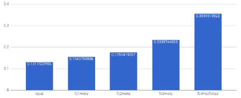
Figure 3: Smoothness analysis of the layer representations of “Urban8K” using the DeepListen [19] fully-connected architecture

Next we present results on image datasets. We trained the network [44] on the CIFAR10 image dataset [8]. As described in [44], the images were cropped to size $24\times 24$. The network has 2 convolution layers (with 9216 and 2304 features, respectively) and 2 fully connected layers (with 384 and 192 features, respectively) with an additional soft-max layer (with final layer ‘logits’ of 10 classes). The training set data size is 50,000 and the testing 10,000. As expected [44], the trained network achieves $86\%$ accuracy on the testing data. In Figure 4 we see a clear indication of how the smoothness begins to evolve during the training after 20 epochs and the ‘unfolding’ of the clustering improves from layer to layer. We also see that the smoothness improves after 50 epochs, correlating with the improvement of the accuracy.

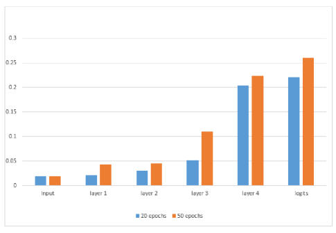
Figure 4: Smoothness analysis of DL layers representations of CIFAR10

We now describe our experiments with the well-known MNIST dataset of 60,000 training and 10,000 testing images [36]. The DL network configuration we used is the ‘textbook’ version of [37], which is composed of two convolution layers and two fully connected layers. Training the model for 100 epochs produce a model with $99.51\%$ accuracy on the training data and a clear monotone increase of Besov smoothness across layers as shown in Figure 5.

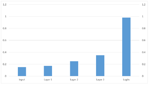
Figure 5: Smoothness analysis of DL layers representations of MNIST

5.2 Smoothness analysis of mis-labeled datasets

Following [49], we applied random mis-labeling to the MNIST and CIFAR10 image sets at various levels. We randomly picked subsets of size $q\%$ of the size of dataset, with $q=10\%,20\%,30\%,40\%$, and then for each image in this subset we picked a random label. We then trained the network of [37] on the misclassified MNIST datasets and the network of [44] on the misclassified CIFAR10 set. We emphasize that the goal of this experiment is to understand generalization [49] and automatically detect the level of corruption solely from the smoothness analysis of the training data. Recall from [49] that a network can converge relatively quickly to an over-fit even on highly mis-classified training sets. Thus, convergence is not a good indication to the generalization capabilities and specifically to the level of mis-labeling in the training data.

Next, we created a wavelet decomposition of RF on the representation of the training set at the last inner layer of the network. Typically, this is the fully connected layer right before the softmax. In Figure 6 we see the decay of the precision error of the adaptive wavelet approximations (2.10) as we add more wavelet terms. It is clear that datasets with less mis-labeling have more ‘sparsity’, i.e., are better approximated with less wavelet terms. We also measured for each mis-labeled training dataset the Besov $\alpha$-smoothness at the last inner layer. The results are presented in Table I. We see a strong correlation between the amount of mis-labeling and the smoothness.

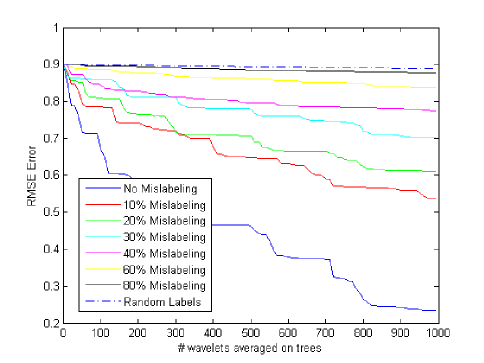
Figure 6: Precision error decay with adaptive wavelet approximation on mis-labeled MNIST

Mis-labeling	0%	10%	20%	30%	40%
MNIST smoothness	0.28	0.106	0.084	0.052	0.03
CIFAR10 smoothness	0.204	0.072	0.053	0.051	0.003

TABLE I: Smoothness analysis of mis-labeled image images

6 Conclusion

In this paper we presented a theoretical approach to the analysis of the performance of the hidden layers in DL architectures. We plan to continue the experimental analysis of deeper architectures and larger datasets (see e.g. [43]) and hope to demonstrate that our approach is applicable to a wide variety of machine learning and deep learning architectures. As some advanced DL architectures have millions of features in their hidden layers, we will need to overcome the problem of estimating representation smoothness in such high dimensions. Furthermore, in some of our experiments we noticed interesting phenomena within sub-components of the layers (e,g, the different operations of convolution, non-linearity and pooling). We hope to reach some understanding and share some insights regarding these aspects too.

[Proof of Theorem 3.7]

Obviously, it is sufficient to prove the equivalence for a single tree $\mathcal{T}$. Observe that condition (3.8) also implies that for any $\Omega^{\prime}\in\mathcal{T}$, with parent $\Omega$, we also have

$$\left|\Omega\right|\leq(1-\rho)^{-1}\left|{\Omega^{\prime}}\right|.$$

We use this as well as (2.5) to prove the first direction of the equivalence as follows

$${{N}_{\tau}}{{\left(f,\mathcal{T}\right)}^{\tau}}=\sum\limits_{{\Omega}^{\prime}\neq{{\Omega}_{0}},{\Omega}^{\prime}\in\mathcal{T}}{\left\|{{\psi}_{{{\Omega}^{\prime}}}}\right\|_{p}^{\tau}}$$

$$=\sum\limits_{\begin{smallmatrix}{\Omega}^{\prime}\neq{{\Omega}_{0}},{\Omega}^{\prime}\in\mathcal{T},\\ \text{ }\Omega\text{ parent of }{\Omega}^{\prime}\end{smallmatrix}}{{{\left({{\left|{{\Omega}^{\prime}}\right|}^{1/p}}{{\left\|{{{\vec{E}}}_{{{\Omega}^{\prime}}}}-{{{\vec{E}}}_{\Omega}}\right\|}_{{{l}_{2}}\left(L-1\right)}}\right)}^{\tau}}}$$

$$=\sum\limits_{{\Omega}^{\prime}\neq{{\Omega}_{0}},{\Omega}^{\prime}\in\mathcal{T}}{{{\left({{\left|{{\Omega}^{\prime}}\right|}^{1/p-1/\tau}}{{\left\|{{\psi}_{{{\Omega}^{\prime}}}}\right\|}_{\tau}}\right)}^{\tau}}}$$

$$\leq c\left(\tau\right)\sum\limits_{\begin{smallmatrix}{\Omega}^{\prime}\neq{{\Omega}_{0}},{\Omega}^{\prime}\in\mathcal{T}\\ ,\Omega\text{ parent of }{\Omega}^{\prime}\end{smallmatrix}}{\left\{{{\left({{\left|{{\Omega}^{\prime}}\right|}^{-\alpha}}{{\left\|{{\left\|f\left(\cdot\right)-{{{\vec{E}}}_{{{\Omega}^{\prime}}}}\right\|}_{{{l}_{2}}\left(L-1\right)}}\right\|}_{{{L}_{\tau}}\left({{\Omega}^{\prime}}\right)}}\right)}^{\tau}}\right.}$$

$$\qquad+\left.{{\left({{\left|{{\Omega}^{\prime}}\right|}^{-\alpha}}{{\left\|{{\left\|f\left(\cdot\right)-{{{\vec{E}}}_{\Omega}}\right\|}_{{{l}_{2}}\left(L-1\right)}}\right\|}_{{{L}_{\tau}}\left({{\Omega}^{\prime}}\right)}}\right)}^{\tau}}\right\}$$

$$\leq c\left(\tau,\rho,\alpha\right)\sum\limits_{\begin{smallmatrix}\Omega\neq{{\Omega}_{0}},,{\Omega}^{\prime}\in\mathcal{T}\\ ,\Omega\text{ parent of }{\Omega}^{\prime}\end{smallmatrix}}{\left\{{{\left({{\left|{{\Omega}^{\prime}}\right|}^{-\alpha}}{{\left\|{{\left\|f\left(\cdot\right)-{{{\vec{E}}}_{{{\Omega}^{\prime}}}}\right\|}_{{{l}_{2}}\left(L-1\right)}}\right\|}_{{{L}_{\tau}}\left({{\Omega}^{\prime}}\right)}}\right)}^{\tau}}\right.}$$

$$\left.\qquad+{{\left({{\left|\Omega\right|}^{-\alpha}}{{\left\|{{\left\|f\left(\cdot\right)-{{{\vec{E}}}_{\Omega}}\right\|}_{{{l}_{2}}\left(L-1\right)}}\right\|}_{{{L}_{\tau}}\left(\Omega\right)}}\right)}^{\tau}}\right\}$$

$$\leq 2c\left(\tau,\rho,\alpha\right)\sum\limits_{\Omega\in\mathcal{T}}{{{\left({{\left|\Omega\right|}^{-\alpha}}{{\left\|{{\left\|f\left(\cdot\right)-{{{\vec{E}}}_{\Omega}}\right\|}_{{{l}_{2}}\left(L-1\right)}}\right\|}_{{{L}_{\tau}}\left(\Omega\right)}}\right)}^{\tau}}}$$

$$=2c\left(\tau,\rho,\alpha\right)\sum\limits_{\Omega\in\mathcal{T}}{{{\left({{\left|\Omega\right|}^{-\alpha}}{{w}_{1}}{{\left(f,\Omega\right)}_{\tau}}\right)}^{\tau}}}$$

$$=c\left|f\right|_{\tilde{B}_{\tau}^{\alpha,1}}^{\tau}.$$

We now prove the other direction. We assume $0<\tau\leq 1$ (the case $1<\tau<\infty$ is similar). For any $\Omega\in\mathcal{T}$ we have

$${{w}_{1}}\left(f,\Omega\right)_{\tau}^{\tau}\leq\sum\limits_{{\Omega}^{\prime}\in\mathcal{T},{\Omega}^{\prime}\subset\Omega}{\left\|{{\psi}_{{{\Omega}^{\prime}}}}\right\|_{\tau}^{\tau}},$$ (.1)

by the following estimates

$${{w}_{1}}\left(f,\Omega\right)_{\tau}^{\tau}=\int_{\Omega}{\left\|\sum\limits_{{\Omega}^{\prime}\in\mathcal{T}}{{{\psi}_{{{\Omega}^{\prime}}}}\left(x\right)}-{{{\vec{E}}}_{\Omega}}\right\|_{{{l}_{2}}\left(L-1\right)}^{\tau}dx}$$

$$\qquad=\int_{\Omega}{\left\|\sum\limits_{{\Omega}^{\prime}\in\mathcal{T}}{{{\psi}_{{{\Omega}^{\prime}}}}\left(x\right)}-\sum\limits_{{\Omega}^{\prime}\in\mathcal{T},\Omega\subseteq{\Omega}^{\prime}}{{{\psi}_{{{\Omega}^{\prime}}}}\left(x\right)}\right\|_{{{l}_{2}}\left(L-1\right)}^{\tau}dx}$$

$$\qquad=\int_{\Omega}{\left\|\sum\limits_{{\Omega}^{\prime}\in\mathcal{T},{\Omega}^{\prime}\subset\Omega}{{{\psi}_{{{\Omega}^{\prime}}}}\left(x\right)}\right\|_{{{l}_{2}}\left(L-1\right)}^{\tau}dx}$$

$$\qquad\leq\sum\limits_{{\Omega}^{\prime}\in\mathcal{T},{\Omega}^{\prime}\subset\Omega}{\left\|{{\psi}_{{{\Omega}^{\prime}}}}\right\|_{\tau}^{\tau}}.$$

Also, observe that by condition (3.8), for any $\Omega^{\prime}\in\mathcal{T}$

$$\sum\limits_{\Omega\in\mathcal{T},{\Omega}^{\prime}\subset\Omega}{{{\left(\frac{\left|{{\Omega}^{\prime}}\right|}{\left|\Omega\right|}\right)}^{\alpha\tau}}}\leq\sum\limits_{k=1}^{\infty}{{{\rho}^{k\alpha\tau}}}\leq c\left(\rho,\alpha,\tau\right).$$ (.2)

We apply (.1) and (.2) to conclude

$$\left|f\right|_{\tilde{B}_{\tau}^{\alpha,1}\left(\mathcal{T}\right)}^{\tau}\leq\sum\limits_{\Omega\in\mathcal{T}}{{{\left|\Omega\right|}^{-\alpha\tau}}\sum\limits_{{\Omega}^{\prime}\in\mathcal{T},{\Omega}^{\prime}\subset\Omega}{\left\|{{\psi}_{{{\Omega}^{\prime}}}}\right\|_{\tau}^{\tau}}}$$

$$=\sum\limits_{\Omega\in\mathcal{T}}{\sum\limits_{{\Omega}^{\prime}\in\mathcal{T},{\Omega}^{\prime}\subset\Omega}{{{\left(\frac{\left|{{\Omega}^{\prime}}\right|}{\left|\Omega\right|}\right)}^{\alpha\tau}}{{\left({{\left|{{\Omega}^{\prime}}\right|}^{-\alpha}}{{\left\|{{\psi}_{{{\Omega}^{\prime}}}}\right\|}_{\tau}}\right)}^{\tau}}}}$$

$$=\sum\limits_{\Omega^{\prime}\neq\Omega_{0},{\Omega}^{\prime}\in\mathcal{T}}{{{\left({{\left|{{\Omega}^{\prime}}\right|}^{-\alpha}}{{\left\|{{\psi}_{{{\Omega}^{\prime}}}}\right\|}_{\tau}}\right)}^{\tau}}\sum\limits_{\Omega\in\mathcal{T},{\Omega}^{\prime}\subset\Omega}{{{\left(\frac{\left|{{\Omega}^{\prime}}\right|}{\left|\Omega\right|}\right)}^{\alpha\tau}}}}$$

$$\leq c\left(\alpha,\tau,\rho\right)\sum\limits_{\Omega^{\prime}\neq\Omega_{0},{\Omega}^{\prime}\in\mathcal{T}}{{{\left({{\left|{{\Omega}^{\prime}}\right|}^{-\alpha}}{{\left|{{\Omega}^{\prime}}\right|}^{1/\tau-1/p}}{{\left\|{{\psi}_{{{\Omega}^{\prime}}}}\right\|}_{p}}\right)}^{\tau}}}$$

$$=c\left(\alpha,\tau,\rho\right)\sum\limits_{\Omega^{\prime}\neq\Omega_{0},{\Omega}^{\prime}\in\mathcal{T}}{\left\|{{\psi}_{{{\Omega}^{\prime}}}}\right\|_{p}^{\tau}}$$

$$=c{{N}_{\tau}}{{\left(f,\mathcal{T}\right)}^{\tau}}.$$

References

- [1] Alani D., Averbuch A. and Dekel S., Image coding using geometric wavelets, IEEE transactions on image processing 16:69-77, 2007.
- [2] Alpaydin E., Introduction to machine learning, MIT Press, 2004.
- [3] Bengio Y., Courville A. and Vincenty P., Representation Learning: A Review and New Perspectives, IEEE Transactions on Pattern Analysis and Machine Intelligence 8:1798-1828, 2013.
- [4] Biau G. and Scornet E., A random forest guided tour, TEST 25(2):197-227, 2016.
- [5] Breiman L., Random forests, Machine Learning 45:5-32, 2001.
- [6] Breiman L., Bagging predictors, Machine Learning 24(2):123-140, 1996.
- [7] Breiman L, Friedman J., Stone C. and Olshen R., Classification and Regression Trees, Chapman and Hall/CRC, 1984.
-
[8]
CIFAR10 image dataset
https://www.cs.toronto.edu/ kriz/cifar.html. - [9] Chen H., Tino P. and Yao X., Predictive Ensemble Pruning by Expectation Propagation, IEEE journal of knowledge and data engineering 21:999-1013, 2009.
- [10] Chollet F., The limitations of deep learning, https://blog.keras.io/the-limitations-of-deep-learning.html, 2017.
- [11] Criminisi A., Shotton J. and Konukoglu E., Forests for Classification, Regression, Density Estimation, Manifold Learning and Semi-Supervised Learning, Microsoft Research technical report, report TR-2011-114, 2011.
- [12] Dahmen W., Dekel S. and Petrushev P., Two-level-split decomposition of anisotropic Besov spaces, Constructive approximation 31:149-194, 2001.
- [13] Daubechies I., Ten lectures on wavelets, CBMS-NSF Regional Conference Series in Applied Mathematics,1992.
- [14] Dekel S., Elisha O. and Morgan O., Wavelet decomposition of Gradient Boosting, submitted.
- [15] Dekel S. and Leviatan D., Adaptive multivariate approximation using binary space partitions and geometric wavelets, SIAM Journal on Numerical Analysis 43:707-732, 2005.
- [16] Denil M., Matheson D. and De Freitas N., Narrowing the gap Random forests in theory and in practice, In Proceedings of the 31st International Conference on Machine Learning 32, 2014.
- [17] DeVore R., Nonlinear approximation, Acta Numerica 7:51-150, 1998.
- [18] DeVore R. and Lorentz G., Constructive approximation, Springer Science and Business, 1993.
-
[19]
DeepListen
https://github.com/jaron/deep-listening - [20] DeVore R., Jawerth B. and Lucier B., Image compression through wavelet transform coding, IEEE transactions on information theory 38(2):719-746, 1992.
- [21] Du W. and Zhan Z., Building decision tree classifier on private data, In Proceedings of the IEEE international conference on Privacy, security and data mining 14:1-8, 2002.
- [22] Elisha O. and Dekel S., Wavelet decompositions of Random Forests - smoothness analysis,sparse approximation and applications, Journal of machine learning research 17: 1-38, 2016.
- [23] Feng N., Wang J. and Saligrama V., Feature-Budgeted Random Forest, In Proceedings of The 32nd International Conference on Machine Learning, 1983-1991, 2015.
- [24] Kelley P. and Barry R., Sparse spatial autoregressions, Statistics and Probability Letters 33(3):291-297, 1997.
- [25] Genuer R., Poggi J. and Christine T., Variable selection using Random Forests, Pattern Recognition Letters 31(14): 2225-2236, 2010.
- [26] Geurts P. and Gilles L., Learning to rank with extremely randomized trees, In JMLR: Workshop and Conference Proceedings 14:49-61, 2011.
- [27] Guyon I. and Elisseff A., An introduction to variable and feature selection, Journal of Machine Learning Research 3:1157-1182, 2003.
- [28] Hastie T., Tibshirani R. and Friedman J., The elements of statistical learning, Springer, 2009.
- [29] Joly A., Schnitzler F.,Geurts P. and Wehenkel L., L1-based compression of random forest models, In Proceedings of the European Symposium on Artificial Neural Networks, Computational Intelligence and Machine Learning, 375-380, 2012.
- [30] Karaivanov B. and Petrushev P., Nonlinear piecewise polynomial approximation beyond Besov spaces, Applied and computational harmonic analysis 15:177-223, 2003.
- [31] Kulkarni V. and Sinha P., Pruning of Random Forest classifiers: A survey and future directions, In International Conference on data science and engineering, 64-68, 2012.
- [32] Loh W., Classification and regression trees, Wiley Interdisciplinary Reviews: Data Mining and Knowledge Discovery 1(1):14-23, 2011.
- [33] Louppe G., Wehenkel L., Sutera A. and Geurts P., Understanding variable importances in forests of randomized trees, Advances in Neural Information Processing Systems 26:431-439, 2013.
- [34] Mallat S., A Wavelet tour of signal processing, 3rd edition (the sparse way), Acadmic Press, 2009.
- [35] Martinez-Muoz G., Hernández-Lobato D. and Suarez A., An analysis of ensemble pruning techniques based on ordered aggregation, IEEE Transactions on pattern analysis and machine intelligence 31:245-259, 2009.
-
[36]
MNIST data set,
http://yann.lecun.com/exdb/mnist/ -
[37]
TensorFlow Tutorial: Deep MNIST for experts,
https://www.tensorflow.org/get started/mnist/pros - [38] Papyan V., Romano Y. and Elad M., Convolutional Neural Networks Analyzed via Convolutional Sparse Coding, Submitted, 2016.
- [39] Raileanu L. and Stoffel K., Theoretical comparison between the Gini index and information gain criteria, Annals of Mathematics and Artificial Intelligence 41(1):77-93, 2004.
- [40] Deep Convolutional Neural Networks and Data Augmentation for Environmental Sound Classification Salamon J. and Bello J. P., IEEE Signal Processing Letters 24(3):279 - 283, 2017.
- [41] Salembier P. and Garrido L., Binary partition tree as an efficient representation for image processing, segmentation, and information retrieval, IEEE transactions on image processing9:561-576, 2000.
- [42] Schwartz-Ziv R. and Tishbi N., Opening the black box of Deep Neural Networks via Information, preprint.
- [43] Sun C., Shrivastava1 A., Singh S. and Gupta1 A., Revisiting Unreasonable Effectiveness of Data in Deep Learning Era, preprint.
-
[44]
AlexaNet implementation using TensorFlow,
https://github.com/tensorflow/models/blob/master/tutorials/image/cifar10/cifar10.py - [45] UCI machine learning repository, http://archive.ics.uci.edu/ml/.
-
[46]
Urban Sound Classification dataset,
https://serv.cusp.nyu.edu/projects/urbansounddataset -
[47]
Urban Sound Classification CNN implementation
https://github.com/jaron/deep-listening/blob/master/4-us8k-cnn-salamon.ipynb - [48] Wavelet-based Random Forest source code, https://github.com/orenelis/WaveletsForest.git.
- [49] Zhang C., Bengio S., Hardt M., Recht B. and Vinyals O., Understanding deep learning requires rethinking generalization, In ICLR 2017 conference proceedings.