Deep Learning Paradigm with Transformed Monolingual Word Embeddings for Multilingual Sentiment Analysis

Abstract

The surge of social media use brings huge demand of multilingual sentiment analysis (MSA) for unveiling cultural difference. So far, traditional methods resorted to machine translation—translating texts in other languages to English, and then adopt the methods once worked in English. However, this paradigm is conditioned by the quality of machine translation. In this paper, we propose a new deep learning paradigm to assimilate the differences between languages for MSA. We first pre-train monolingual word embeddings separately, then map word embeddings in different spaces into a shared embedding space, and then finally train a parameter-sharing deep neural network for MSA. The experimental results show that our paradigm is effective. Especially, our CNN model outperforms a state-of-the-art baseline by around 2.1% in terms of classification accuracy.

1 Introduction

The prevalence of social media has allowed for the collection of abundant subjective multilingual texts. Twitter is a particularly significant multilingual data source that provides researchers with sufficient opinion pieces on various topics from all over the world. An analysis of these multilingual opinion texts can reveal the cultural variations in public opinions from different areas. Therefore, an efficient multilingual sentiment analysis (MSA) that can process all multilingual texts (mixed monolingual texts) simultaneously is necessary.

There has been substantial research on monolingual sentiment analysis, including sentiment analysis of traditional reviews (product/movie, etc.; Pang et al. (2002); Turney (2002); Pang and Lee (2008)) and tweets (Agarwal et al. (2011); Go et al. (2009); Xiang and Zhou (2014); Mukherjee and Bhattacharyya (2012)). Instead of creating separate models for each language, an MSA should use a single model (with the same parameters for all languages) to process different texts in different languages.

However, compared with monolingual sentiment analysis, the research on MSA has progressed slowly. One of the reasons for this is that there is no benchmark dataset that supports the evaluation of MSA methods (particularly, its cross-language adaptability). As many previous studies have highlighted, open-source sentiment datasets are imbalanced Mihalcea et al. (2007); Denecke (2008); Wan (2009); Steinberger et al. (2011): there are many freely available annotated sentiment corpora for English; however, such corpora for other languages are scarce or even nonexistent. As a compromise, many of the previous multilingual corpora have been built using human/machine translations, which are unrealistic.

In this study, we used the MDSU corpus as our training/test dataset Lu et al. (2017). The MDSU corpus contains three distinct languages (i.e., English, Japanese, and Chinese) and four identical international topics (i.e., iPhone 6, Windows 8, Vladimir Putin, and Scottish Independence), with 5,422 tweets in total. The multilinguality of the corpus makes it the most suitable training/test dataset for MSA.

Moreover, traditional machine learning methods that are effective in monolingual settings are not necessarily effective in multilingual settings, because they usually require heavy language-specific feature engineering that further needs language-specific resources (e.g., polarity lexicons)/tools (e.g., POS taggers and parsers). This prevents the application of many sophisticated monolingual methods to other languages, particularly the minor languages that lack basic NLP tools. Until now, the most typically used methods of MSA have been based on machine translation (MT): first, texts in other languages are translated into English, and then machine-learning methods are developed based on the expanded English texts.

However, this paradigm is conditioned strongly by the quality of the MT. Considering that our processing objects—tweets—contain many informal expressions, it is even more difficult to guarantee an accurate MT. Therefore, we proposed a new deep learning paradigm to integrate the processing of different languages into a unified computation model. First, we pre-trained monolingual word embeddings separately; second, we mapped them in different spaces within a shared embedding space; and finally, we trained a parameter-sharing deep neural network for MSA. Our model is presented in Figure 1.

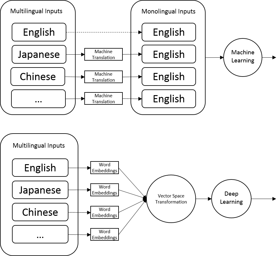
Figure 1: MT-Based Paradigm and Deep Learning Paradigm

Although the study by Ruder et al. (2016) is most similar to ours in the use of deep learning methods, there are two fundamental differences. First, they only input the raw monolingual word embeddings (an open-source, pre-trained word embedding for English and random word embeddings for other languages) in their deep learning methods; however, we used customized pre-trained word embeddings and further transferred them into a shared space. Second, they created separate models for each language, whereas we developed a single parameter-sharing model for all languages.

To the best of our knowledge, this study is the first to use a deep learning paradigm for MSA. Moreover, because of the use of such a paradigm, the only resources we required were word embeddings for each language and tokenizers for non-spaced languages (e.g., Chinese). We expected this paradigm to assimilate language differences to take full advantage of the size of multilingual datasets (compared with its smaller monolingual parts). In this study, we employed the LSTM and CNN models. Our parameter-sharing CNN model with adjusted word embeddings outperformed the machine-translation-based baseline by nearly 5.3% and the state-of-the-art baseline by 2.1%, thereby proving its effectiveness.

This paper is organized as follows: in Section 2, we discuss the related studies; in Section 3, we describe the study methods; in Section 4, we presented and discussed the results of the experiments; and finally, in Section 5, we draw conclusions.

2 Related Work

In this section, we introduce MSA-related studies, including those on multilingual subjectivity analysis as well as the MSA of traditional text and social media.

2.1 Multilingual Subjectivity Analysis

Sentiment analysis in a multilingual framework was first conducted for subjectivity analysis. Mihalcea et al. Mihalcea et al. (2007) explored the automatic generation of resources (i.e., lexicon translation and corpus projection) for the subjectivity analysis of a new language (i.e., Romanian). They translated the English polarity lexicon into the target language, assessed the quality of the generated lexicon through an annotation study, and proposed a rule-based target-language classifier using the generated lexicon. The results revealed that the translated lexicon was less reliable compared with the English one, and the performance of the rule-based subjectivity classifier was worse in Romanian than in English. They also conducted a subjectivity annotation on a parallel corpus (English sentences were manually translated to Romanian); the results indicated that in most cases, the subjectivity was preserved during the translation. They projected the subjectivity onto the Romanian part to automatically obtain a Romanian subjectivity corpus and trained Naive Bayes (NB) classifiers. The results revealed that the performance of the NB classifiers in Romanian was worse than in English.

Banea et al. Banea et al. (2010) translated the English corpus into other languages (i.e., Romanian, French, English, German, and Spanish) and explored the integration of unigram features from multiple languages into a machine learning approach for subjectivity analysis. They demonstrated that both English and the other languages could benefit from using features from multiple languages. They believed that this was probably because, when one language does not provide sufficient information, another one can serve as a supplement.

2.2 MSA of Traditional Text

Although there is extensive scope for improvement, translation-based methods have inspired many other studies. The research on MSA began relatively late. Denecke Denecke (2008) translated German movie reviews into English, developed SentiWordNet-based methods for English movie reviews, and tested the proposed methods on the German corpus. The results revealed that the performance of the proposed methods in MSA was similar to that in monolingual settings. Wan Wan (2009) leveraged a labeled English corpus for Chinese sentiment classification. He first machine translated the labeled English corpora and an unlabeled Chinese corpus to the target language, and then proposed a co-training approach to use the unlabeled corpora. His experimental results suggested that the co-training approach outperformed the standard inductive and transductive classifiers. Steinberger et al. Steinberger et al. (2011) annotated entity-opinion pairs in a parallel news article corpus in seven European languages—English, Spanish, French, German, Czech, Italian, and Hungarian (they first did the annotation work for English and then projected those annotations onto other languages). Their simple method to determine the word polarity aggregation for entity-level sentiment analysis was tested on the entity-opinion pairs in the parallel corpus. They created a valuable resource for entity-level sentiment analysis in a multilingual setting; however, their method, as they observed, is preliminary and depends substantially on language-specific polarity lexicons.

2.3 MSA of Social Media

Recently, the MSA of social media content has been increasing. Balahur and Turchi Balahur and Turchi (2013) conducted an MSA of tweets. They first translated English tweets into four languages—Italian, Spanish, French, and German (the texts in the test set were further corrected manually) to create an artificial multilingual corpus. They then tested support vector machine (SVM) classifiers using polarity lexicon-based features on various combinations of the dataset in different languages. The results suggested that the combined use of training data from multiple languages improves the performance of sentiment classification. Volkova et al. Volkova et al. (2013) constructed a multilingual tweet dataset in English, Spanish, and Russian using Amazon Mechanical Turk. They explored the lexical variations in subjective expression and the differences in emoticon and hashtag usage by gender information in the three different languages; their results demonstrated that gender information can be used to improve the performance sentiment analysis of all the three languages.

2.4 Comparison with Previous Work

Our study is different from the previous studies in the following ways. First, in multilingual datasets from previous studies, datasets of languages other than English have been projected from the English dataset. Banea et al. Banea et al. (2010) and Balahur and Turchi Balahur and Turchi (2013) have used MT to obtain texts in target languages, which are considerably noisy. Mihalcea et al. Mihalcea et al. (2007) and Dwnwcke Denecke (2008) have directly used parallel corpora to eliminate this noise. However, real multilingual opinion texts would not be in the form of parallel corpora because users usually give their opinions in one language. Therefore, the MDSU corpus in this study includes three distant languages and covers common international topics, which is useful to test the multilingual adaptability of a method.

As for methods, Denecke Denecke (2008) and Wan Wan (2009) have adopted the “MT + machine learning” approach, which unavoidably imports bias during the MT. The abstraction of the word feature in Balahur and Turchi Balahur and Turchi (2013) can be applied to other languages, but it requires language-specific polarity lexicons. Banea et al. Banea et al. (2010) used unigrams in multiple languages as features, but they might be restricted due to data sparseness issues. Volkova et al. Volkova et al. (2013) proved the effectiveness of employing gender information, but their classifiers are not designed for multilingual settings. By contrast, our deep learning methods require no polarity lexicons and can unify different languages through a neural text model that uses word embeddings.

3 Methods

In this section, we introduce our baseline methods and the proposed deep learning methods (i.e., transformed word embedding + deep learning). The global polarity of the MDSU corpus has three types: positive, negative, and neutral; therefore, our study is technically a three-way classification task.

3.1 Baselines

Our first baseline was MT-based. We used Google Translate to translate Japanese/Chinese tweets into English. Google Translate is a paid service that supports more than 100 languages at various levels. For Japanese and Chinese, neural MT technology was enabled, providing more reliable translation results for the baselines.

The SVM-based learning methods with n-gram features, proposed by Pang et al. Pang et al. (2002) and Go et al. Pang et al. (2002), have been frequently used as baselines in many monolingual (English) studies. Similar to their settings, we used the default SVM model with a linear kernel and $C=1$ and fed the binarized unigram/bigram term frequencies as features. The one-vs-one strategy was adopted for multiclass classification. Following the traditional paradigm, the SVM model trained on all translated tweets in the MDSU corpus is our first baseline, denoted as MT-SVM.

In addition, we re-implemented Banea et al.’s Banea et al. (2010) NB model that uses the cumulation of monolingual unigram features. We fine tuned Banea et al.’s method in two ways: first, we used both unigram and bigram as our features; and second, we used all the features instead of parts of them. We denoted this state-of-the-art baseline that does not use language-specific polarity lexicons as Banea (2010)*.

3.2 Deep Learning Paradigm

3.2.1 Space Transformation by Translation Matrix

Since there is no comparable open source word embeddings learnt from Twitter data for multiple languages, we independently obtained word embeddings using numerous monolingual texts for each language. However, these monolingual word embeddings were heterogeneous in terms of vector space (the meaning of each dimension was different between languages.). Hence, we attempted to reduce the discrepancy between monolingual word embeddings.

This notion was adopted from Mikolov et al. Mikolov et al. (2013). In their study, they highlighted that the same concepts have similar geometric arrangements in their respective vector spaces. This implies that if the matrix transformation is adequately performed, monolingual word embeddings in heterogeneous spaces can be adjusted to a shared vector space. Thereafter, many other ways to conduct this transformation have been proposed Ruder (2017). Following Mikolov et al. Mikolov et al. (2013), we used the Translation Matrix method—to obtain a linear projection between the languages using a set of pivot word pairs.

Assume a set of word pairs $\{{\bf x}_{i},{\bf z}_{i}\}_{i=1}^{n}$, where ${\bf x}_{i}$ and ${\bf z}_{i}$ are the vector representations of word $i$ in the source and target languages, respectively. We aimed to identify a translation matrix ${\bf W}_{S\rightarrow T}$ that minimized the following object function:

$$\mathop{\rm minimize}\limits_{{\bf W}_{S\rightarrow T}}\ \sum_{i=1}^{n}||{\bf W}_{S\rightarrow T}{\bf x}_{i}-{\bf z}_{i}||^{2}$$ (1)

After ${\bf W}_{S\rightarrow T}$ was identified, we mapped the vocabulary matrix ${\bf Z}$ of one language space to another by computing ${\bf\hat{Z}}={\bf Z{\bf W}_{S\rightarrow T}}$. For example, we transferred the Japanese vocabulary matrix to the English vector space using $\hat{{\bf Z}}_{J}={\bf Z}_{J}{\bf W}_{J\rightarrow E}$.

In this paper, we developed two types of translation matrix: ${\bf W}_{J\rightarrow E}$ and ${\bf W}_{C\rightarrow E}$, to unify our separately pre-trained monolingual word embeddings into a shared one. We selected top $K$ high-frequent word in the English training corpus as our pivot words, translated them into Japanese and Chinese (using Google Translate), and finally obtained the translation matrices using a linear regression algorithm.

Although the linear projection by the Translation Matrix method can be considered as a word-level MT, the space transformation is considerably less expensive than building a full-fledged MT system.

3.2.2 LSTM

RNNs have received tremendous attention in the NLP field and been employed to complete many tasks, including predicting words/phrases, speech recognition, image caption generation, and MT.

Traditional neutral networks are stateless, whereas RNNs have the unique property of being “stateful”. By reusing the hidden units in the previous layer, RNNs allow cyclically encoding of past information within the networks.

Let ${\bf x}_{i}\in\Re^{k}$ be the $k$-dimensional word vector corresponding to the $i$-th word in a tweet; then, a tweet having n words can be represented as ${\bf X}=({\bf x}_{1},...,{\bf x}_{T})$. At each time step $t$, the hidden state ${\bf h}_{t}$ of the RNN is updated as follows:

$${\bf h}_{t}=f({\bf h}_{t-1},{\bf x}_{t})$$ (2)

where $f$ is a function that takes a signal ${\bf x}_{t}$ as input during time step $t$, updates its current state ${\bf h}_{t}$ based on the influence of ${\bf x}_{t}$ and the previous state ${\bf h}_{t-1}$.

A vanilla RNN only combines the precious hidden state ${\bf h}_{t}$ with the current input ${\bf x}_{t}$, which is not powerful enough to present a complex context. Thus, we used an LSTM network instead.

The LSTM model introduces a new structure called a memory block (see Figure 2). A memory block consists of four main elements: input, output, and forget gates and a self-connected cell. The cell is at the center of the LSTM memory block. Gates can be regarded as water valves, which yield values between 0 and 1, describing how much of each component should be let through. An LSTM memory block has three of these gates, to modulate the cell state.

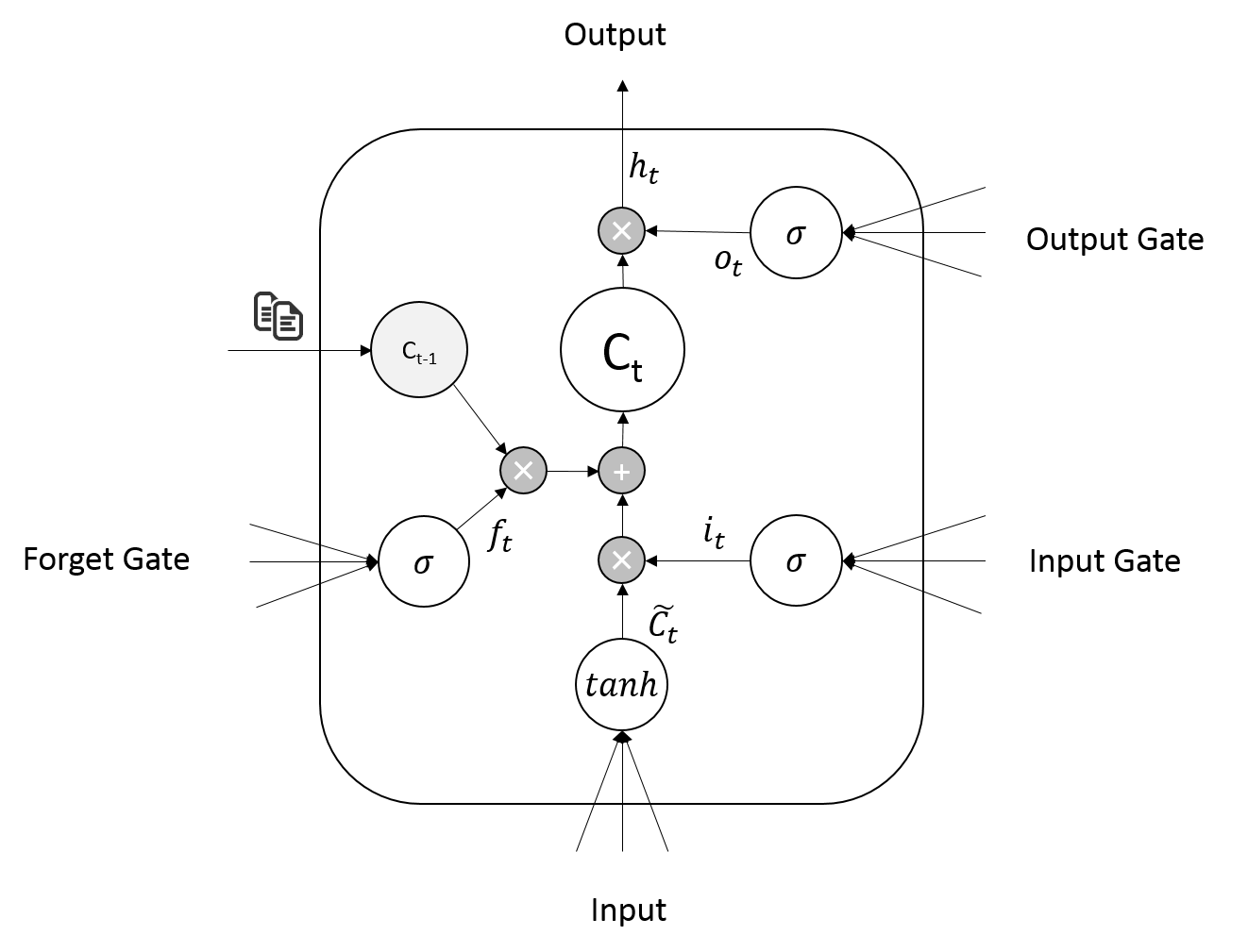
Figure 2: LSTM Memory Block

Specifically, the input gate ${\bf i}_{t}$ controls the candidate state of the cell $\tilde{{\bf C}_{t}}$; the forget gate ${\bf f}_{t}$ regulates the previous state of the cell ${\bf C}_{t-1}$; and the output gate ${\bf o}_{t}$ determined the parts of the cell state ${\bf C}_{t}$ to output.

Eqs.(3)–(8) describe how a layer of memory blocks is updated at every time step $t$.

$${\bf i}_{t}=\sigma({\bf W}_{i}{\bf x}_{t}+{\bf U}_{i}{\bf h}_{t-1}+{\bf b}_{i})$$ (3)

$${\tilde{\bf C}_{t}}=\sigma({\bf W}_{c}{\bf x}_{t}+{\bf U}_{c}{\bf h}_{t-1}+{\bf b}_{c})$$ (4)

$${\bf f}_{t}=\sigma({\bf W}_{f}{\bf x}_{t}+{\bf U}_{f}{\bf h}_{t-1}+{\bf b}_{f})$$ (5)

$${\bf C}_{t}={\bf i}_{t}*{\tilde{\bf C}_{t}}+{\bf f}_{t}*{\bf C}_{t-1}$$ (6)

$${\bf f}_{o}=\sigma({\bf W}_{o}{\bf x}_{t}+{\bf U}_{o}{\bf h}_{t-1}+{\bf b}_{o})$$ (7)

$${\bf h}_{t}={\bf o}_{t}*tanh({\bf C}_{t})$$ (8)

where ${\bf x}_{t}$ is the input to the memory block layer at time $t$, ${\bf W}_{i}$,${\bf W}_{c}$,${\bf W}_{f}$,${\bf W}_{o}$,${\bf U}_{i}$,${\bf U}_{c}$,${\bf U}_{f}$,${\bf U}_{o}$ are weight matrices, and ${\bf b}_{i}$,${\bf b}_{c}$,${\bf b}_{f}$,${\bf b}_{o}$ are bias vectors.

Although LSTM memory blocks have a unique (more complicated) way of computing the hidden state, they use the same network structure as the RNN. The lengths of both hidden layer and cell layer for LSTM take the same value as the dimensionality of word embeddings.

3.2.3 CNN

There have been continual debates on which model—the RNN or CNN—is more suited for NLP tasks Yin et al. (2017). Therefore, we use a CNN model for MSA as well.

One of the advantages of CNNs is that they have much fewer parameters than fully connected networks with the same number of hidden units, which makes them much easier to be trained. Our CNN is similar to that of Kim Kim (2014). Our CNN model is presented in Figure 3.

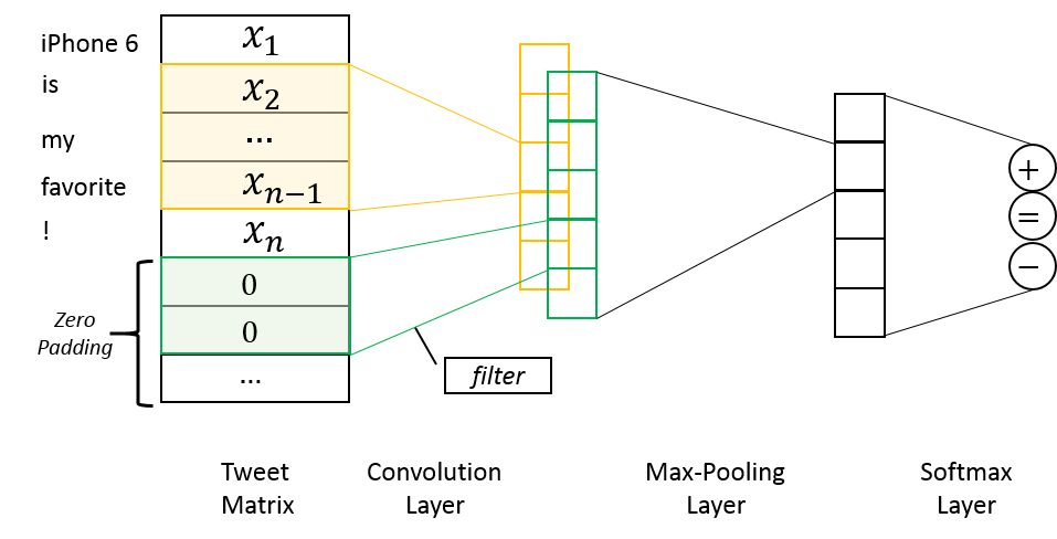
Figure 3: Network Structure of the CNN Model

As in RNNs, a tweet having n words was represented as follows:

$${\bf x}_{1:n}={\bf x}_{1}\oplus{\bf x}_{2}\oplus{\bf x}_{3}\oplus...\oplus{\bf x}_{n}$$ (9)

where $\oplus$ is the concatenation operator. Here, the final index of the word vectors in a tweet was $n$ instead of $T$. In general, ${\bf x}_{i:i+j}$ meant the concatenation of words ${\bf x}_{i},{\bf x}_{i+1},...,{\bf x}_{i+j}$.

To unify the matrix representation of tweets in different length, the maximum length of all tweets in the dataset was used as the fixed size for tweet matrices. For shorter tweets, zero word vectors were padded at the back of a tweet matrix.

The layers of the CNN are formed by a convolution operation followed by a pooling operation. First, we performed a convolution operation to transform a window of $h$ words (i.e., ${\bf x}_{i:i+h-1}$) to generate a feature $c_{i}$. The procedure was formulated as follows:

$$c_{i}=\sigma({\bf w}\cdot{\bf x}_{i:i+h-1}+b)\\$$ (10)

where ${\bf w}$ denotes a filter map, h is the window size of a filter, $\sigma$ is a non-linear activation function and $b$ is a bias term.

By applying filter ${\bf w}$ to each possible window of words in a sentence, we obtained a feature map:

$${\bf c}=[c_{1},c_{2},...,c_{n-h+1}]$$ (11)

Second, we performed a subsampling operation, for which we used the following max-pooling subsampling method based on the idea of capturing the most important feature from each feature map.

$$c_{max}=max\{{\bf c}\}$$ (12)

From Eqs. (10)–(12), a filter generated one $c_{max}$ from a tweet matrix.

The number of filter maps in our CNN model was 100, and the possible window sizes were $\{3,4,and5\}$; thus, our model had 300 different filters in total. The corresponding 300 $c_{max}$ formed the penultimate layer, and was then passed to a fully connected softmax layer to predict the global polarity of a tweet.

4 Experiments

In this section, we compare our deep learning methods with the baseline methods. We first describe our experimental setup, followed by a discussion of the results.

4.1 Experimental Setup

4.1.1 Datasets

As described in Section 1, we used the MDSU corpus as our training/test dataset. The MDSU corpus was originally built for deeper sentiment understanding in a multilingual setting; therefore, tweets in it were annotated many fine-grained tags in addition to global (overall) polarity. In this paper, we used global polarities as the classification labels. Lu et al. (2017) filtered out apparent non-emotional tweets and prioritized long tweets with rich language phenomenon during data selection; therefore, the tweets in the MDSU corpus are more complex and longer than those in randomly collected or noisy-labeled tweet datasets.

Table 1 presents the global polarity distribution for each language in the MDSU corpus. The polarity distribution of each language although not perfectly uniform, does not differ largely. Moreover, the polarity distribution of the entire corpus is well-balanced, rendering it a suitable corpus for a three-way sentiment classification. The length of a tweet is defined as the number of elements (including words, emoticons, and punctuations) after under-mentioned preprocessing. The maximum length (also the fixed size of the CNN models) of the MDSU corpus is 124: 41 for English, 93 for Japanese, and 124 for Chinese.

Table 1: Polarity Distribution for Each Language in the MDSU Corpus

Language	Abbr.	Positive	Neutral	Negative	Total #	Max Length
English	EN	503	526	774	1803	41
Japanese	JA	392	875	534	1801	93
Chinese	ZH	566	614	638	1818	124
Total	ALL	1461	2015	1946	5422	124

4.1.2 Preprocessing

The language used in social media is more casual than in traditional media. There are many unique ways of expression on Twitter, such as emoticons, Unicode emojis, misspelled words, letter-repeating words, all-caps words, and special tags (e.g., #, @). These may disturb the learning of word embeddings and classification models; therefore, we preprocessed them to unify the elements in different shapes but with same meanings as much as possible.

For all the three languages, we detected Unicode emojis and replaced them with an “EMOJI_CODE” (e.g., we replaced “” with “EMOJI_2764”); detected emoticons from easy :-) to complex (((o (*${}^{\circ}\bigtriangledown^{\circ}$*) o)))) using regular expressions and replaced them with “EMOTICON”; and labeled URLs as “URL”).

We also performed language-dependent preprocessing. For English, we lowercased English characters and tokenized the tweets with TweetTokenizer; for Japanese, we normalized Japanese characters and tokenized the tweets with Mecab; for Chinese, we transferred traditional Chinese characters to simplified Chinese characters and tokenized the tweets with NLPIR.

4.1.3 Word Embeddings and Translation Matrix

In addition to the annotated MDSU corpus, we accumulated large collections of raw tweets using Twitter RESTful API by the same query keywords during a one-year period. We first excluded undesirable tweets (e.g., tweets starting with “RT”) using the same veto patterns as Lu et al. (2017); then, we checked the preceding 10 tweets to delete the repeating tweets, because similar tweets usually appear in succession. After filtering out the undesirable tweets, the remaining tweets were preprocessed as previously described. The number of remaining tweets was 232,214 (EN), 264,179 (JA), and 148,052 (ZH). The vocabulary size for each collection of tweets was 63,343 (EN), 49,575 (JA), and 52,292 (ZH).

Our vector representation for words was learnt using FastText. Because the scale of our corpus for word embedding training was relatively small, we set the minimal number of word occurrences as 2. We used the skip-gram model because it generates higher quality representations for infrequent words Mikolov et al. (2013). The word embeddings for each language were trained separately on its corresponding corpus. Words that were not present in the pre-trained word list were initialized randomly in the deep learning models.

The dimensionality of our word embeddings was 100, and the Japanese/Chinese spaces were transformed by their respective translation matrices. For the translation matrix, we set k as 3500, which implied that the top 3500 English words and their translations were the pivot word pairs. We split the 3500 pivot word pairs into two sets—training set (3000 words) and test set (500 words). The translation matrices were obtained based on the training sets. As a validation, we calculated the change of Euclidean/cosine distances for each word pair in the test set before and after the mapping; Table 2 depicts the decrease in the sum of the two distances.

Table 2: Sum of Embedding Distances of Word Pairs in the Test Set

Language		Before Mapping	After Mapping
Japanese	Euclidean Distance	2,455.94	2,135.51
	Cosine Distance	458.37	440.82
Chinese	Euclidean Distance	2,457.05	2,098.76
	Cosine Distance	496.01	490.88

4.1.4 Model Hyper-parameters

All the methods were tested using 10-fold cross validation. For the deep learning models, we randomly selected 10% of the training splits of cross-validation as the developed datasets to tune parameters for an early stopping.

For fair comparison, we empirically set the hyper-parameters for deep learning models as consistent as possible. Both trainings were completed using a stochastic gradient descent (SGD) algorithm for shuffled mini-batches with the Adadelta update rule, with a mini-batch size of 50. The dropout technique is effective in preventing co-adaptation of hidden units by randomly setting a portion of the hidden units to zeroes during feedforward/backpropagation. Therefore, to prevent overfitting, we employed the dropout technique for both deep learning models on their penultimate softmax layers, with a dropout rate of 0.5. We did the same for the dimensionality of word embeddings; the lengths of both the hidden and cell layer for LSTM were 100.

4.2 Result and Discussion

4.3 Baselines

Table 3 presents the classification accuracies of baselines.

According to Table 3, the average accuracy of separate SVM classifiers over original datasets was the same as it over translated datasets. This showed that the same method did not necessarily perform worse after being translated by MT for monolingual datasets. In addition, the performance of MT+SVM model (use all translated tweets) was worse than the average accuracy of separate SVM classifiers over original datasets (53.0% vs. 54.5%), showing the limitation of traditional paradigm(i.e., “MT + machine learning”).

For classifiers directly used the cumulation of unigram and bigram, both SVM and Banea (2010)* performed better than MT+SVM by 0.8% and 3.4%, respectively. The increases indicate that the use of cumulation of n-gram is effective; although this may result in the problem of data sparseness Banea et al. (2010), it could be mitigated by feature selection.

Table 3: Results of Baselines

Model	Dataset	Feature	Accuracy
Average	–	–	0.545
SVM	EN	unigram+bigram	0.529
SVM	JA	unigram+bigram	0.596
SVM	ZH	unigram+bigram	0.509
Average	–	–	0.545
SVM	EN	unigram+bigram	0.529
SVM	Translated JA	unigram+bigram	0.591
SVM	Translated ZH	unigram+bigram	0.515
MT+SVM	Translated ALL	unigram+bigram	0.530
SVM	ALL	cumulation of unigram+bigram	0.538
Banea (2010)*	ALL	cumulation of unigram+bigram	0.564

4.4 Deep Learning Methods

Table 4 presents the classification accuracies of the deep learning models; the input of word embeddings for the models in this Table involved no transformation.

First, our deep learning paradigm performs better than the MT+SVM method (traditional paradigm). Specifically, parameter-sharing LSTM and CNN models outperformed MT+SVM model by 1.2% and 4.3%, respectively. Thus, the deep learning paradigm is more efficient than the traditional paradigm. In addition, the LSTM performed worse than the Banea (2010)* baseline, whereas the CNN excelled. Thus, CNN is more suitable for MSA than LSTM.

Besides, we also conducted the learning separately on each language split. The results revealed that the average accuracies of separate LSTM/CNN classifiers were a little higher than the accuracy of the mixed case (54.4% vs. 54.2%, and 58.1% vs. 57.3%), implying that the deep learning methods did not improve after using the entire dataset. This was a result of the heterogeneity of vector spaces of word embeddings, because the raw word embeddings were learned separately.

Furthermore, we observed that both MT + LSTM and MT + CNN models (trained on the translated datasets and using only English word embeddings) performed worse than the LSTM and CNN models (trained on the original datasets and using multilingual word embeddings). Ideally, if JA/ZH were perfectly translated, the performance should have increased. This suggests that the noises that MT brings in are greater than the heterogeneity of multilingual word embeddings does.

Table 4: Results of Deep Learning Models

Model	Dataset	Accuracy
Average	–	0.544
LSTM	EN	0.531
LSTM	JA	0.569
LSTM	ZH	0.532
MT+LSTM	Translated ALL	0.541
Parameter-sharing LSTM	ALL	0.542
Average	–	0.581
CNN	EN	0.578
CNN	JA	0.610
CNN	ZH	0.553
MT+CNN	Translated ALL	0.564
Parameter-sharing CNN	ALL	0.573

4.5 Deep Learning Methods using Transformed Word Embeddings

The unification of different vector spaces was expected to further improve the deep learning paradigm. Table 5 presents the classification accuracies of the deep learning models before and after space coordination. According to Table 5, the effectiveness of LSTM and CNN models were divided. We observed that after space transformation, the accuracy of LSTM decreased by 0.6%, whereas the accuracy of CNN increased by 1.4%. This suggests that the same vector space transformation does not necessarily suitable for different kinds of network structures.

Overall, the performance of the CNN model fed with transformed word embeddings was most effective.

Table 5: Results of Deep Learning Models Before and After Space Transformation

Model	Dataset	Word Embedding	Accuracy
Parameter-sharing LSTM	ALL	Raw (Table 4)	0.542
	ALL	Transformed	0.536
Parameter-sharing CNN	ALL	Raw (Table 4)	0.573
	ALL	Transformed	0.587

5 Conclusion and Future Work

In this paper, we proposed a novel deep learning paradigm for MSA. We map monolingual word embeddings into a shared embedding space, and used parameter-sharing deep learning models to unify the processing of multiple languages. The tests on a well-balanced tweet sentiment corpus—the MDSU corpus—revealed the effectiveness of our deep learning paradigm. Especially, our CNN model fed with translation matrix-transformed word embeddings achieves a rise of 2.3%, comparing with the strong Banea (2010)* baseline.

Our paradigm provides a great cross-lingual adaptability. Training tweets in any other language can be transferred into vector representation using transformed word embeddings, and then combined with the learning process of the deep learning models.

The novelty of our study is not in the complexity of the network itsel, but more in the unification of heterogeneous monolingual word embeddings and the parameter-sharing model for multilingual datasets. In the future, we plan to attempt more complex transformation methods and network structures.

References

- Agarwal et al. (2011) Apoorv Agarwal, Boyi Xie, Ilia Vovsha, Owen Rambow, and Rebecca Passonneau. 2011. Sentiment analysis of twitter data. Proceedings of the Workshop on Language in Social Media (LSM 2011) pages 30–38.
- Balahur and Turchi (2013) Alexandra Balahur and Marco Turchi. 2013. Improving sentiment analysis in twitter using multilingual machine translated data. In Proceedings of Recent Advances in Natural Language Processing pages 49–55.
- Banea et al. (2010) Carmen Banea, Rada Mihalcea, and Janyce Wiebe. 2010. Multilingual subjectivity: Are more languages better? In Proceedings of the 23rd International Conference on Computational Linguistics (COLING 2010) pages 28––36.
- Carrier and Cho (2017) Pierre Luc Carrier and Kyunghyun Cho. 2017. Lstm networks for sentiment analysis. http://deeplearning.net/tutorial/lstm.html. [Online; accessed May 10, 2017].
- Chang and Lin (2011) Chih-Chung Chang and Chih-Jen Lin. 2011. Libsvm: A library for support vector machine. ACM Transactions on Intelligent Systems and Technology 2(3). Article No. 27.
- Denecke (2008) Kerstin Denecke. 2008. Using sentiwordnet for multilingual sentiment analysis. In Proceedings of the 24th International Conference on Data Engineering Workshop (ICDE 2008) pages 507––512.
- Elman (1990) Jeffrey L Elman. 1990. Finding structure in time. Cognitive Science 14(2):179––211.
- Go et al. (2009) Alec Go, Richa Bhayani, and Lei Huang. 2009. Twitter sentiment classification using distant supervision. CS224N Project Report (Stanford) pages 1–6.
- Kim (2014) Yoon Kim. 2014. Convolutional neural networks for sentence classification. Proceedings of the 2014 Conference on Empirical Methods in Natural Language Processing (EMNLP) pages 1746–1751.
- Lu et al. (2017) Yujie Lu, Kotaro Sakamoto, Hideyuki Shibuki, and Tatsunori Mori. 2017. Construction of a multilingual annotated corpus for deeper sentiment understanding in social media. Journal of Natural Language Processing 24(2):205––266.
- Mihalcea et al. (2007) Rada Mihalcea, Carmen Banea, and Janyce Wiebe. 2007. Learning multilingual subjective language via cross-lingual projections. In Proceedings of the 45th Annual Meeting of the As-sociation of Computational Linguistics (ACL 2007) pages 976––983.
- Mikolov et al. (2010) Tomas Mikolov, Martin Karafiat, Lukas Burget, JanCernocky, and Sanjeev Khudanpur. 2010. Recurrent neural network based language model. INTERSPEECH pages 1045––1048.
- Mikolov et al. (2013) Tomas Mikolov, Quoc V. Le, and Ilya Sutskever. 2013. Exploiting similarities among languages for machine translation. arXiv:1309.4168 .
- Mukherjee and Bhattacharyya (2012) Subhabrata Mukherjee and Pushpak Bhattacharyya. 2012. Sentiment analysis in twitter with lightweight discourse analysis. Proceedings of the 23th International Conference on Computational Linguistics: Technical Papers (COLING 2012) pages 1847–1864.
- Pang and Lee (2008) Bo Pang and Lillian Lee. 2008. Opinion mining and sentiment analysis. Now Publishers.
- Pang et al. (2002) Bo Pang, Lillian Lee, and Shivakumar Vaithyanathan. 2002. Thumbs up? sentiment classification using machine learning techniques. Proceedings of Empirical Methods on Natural Language Processing (EMNLP 2002) pages 79–86.
- Ruder (2017) Sebastian Ruder. 2017. A survey of cross-lingual embedding models. arXiv:1706.04902 .
- Ruder et al. (2016) Sebastian Ruder, Parsa Ghaffari, and John G. Breslin. 2016. Insight-1 at semeval-2016 task 5: Deep learning for multilingual aspect-based sentiment analysis. In Proceedings of Proceedings of SemEval-2016 pages 330––336.
- Steinberger et al. (2011) Josef Steinberger, Polina Lenkova, Mijail Kabadjov, Ralf Steinberger, and Erik van der Goot. 2011. Multilingual entity-centered sentiment analysis evaluated by parallel corpora. Proceedings of Recent Advances in Natural Language Processing pages 770–775.
- Turney (2002) Peter D. Turney. 2002. Thumbs up or thumbs down?: Semantic orientation applied to unsupervised classification of reviews. ACL ’02 Proceedings of the 40th Annual Meeting on Association for Computational Linguistics pages 417–424.
- Volkova et al. (2013) Svitlana Volkova, Theresa Wilson, and David Yarowsky. 2013. Exploring demographic language variations to improve multilingual sentiment analysis in social media. Proceedings of the 2013 Conference on Empirical Methods in Natural Language Processing (EMNLP 2013) pages 1815–1827.
- Wan (2009) Xiaojun Wan. 2009. Co-training for cross-lingual sentiment classification. In Proceedings of the Joint Conference of the 47th An-nual Meeting of the ACL and the 4th International Joint Conference on Natural Language Processing of the AFNLP pages 235––243.
- Wang and Raj (2017) Haohan Wang and Bhiksha Raj. 2017. On the origin of deep learning. arXiv:1702.07800v4 .
- Xiang and Zhou (2014) Bing Xiang and Liang Zhou. 2014. Improving twitter sentiment analysis with topic-based mixture modeling and semi-supervised training. Proceedings of the 52nd Annual Meeting of the Association for Computational Linguistics (Short Papers)(ACL’14) pages 434–439.
- Yin et al. (2017) Wenpeng Yin, Katharina Kann, Mo Yu, and Hinrich Schütze. 2017. Comparative study of cnn and rnn for natural language processing. arXiv:1702.01923 .