Numerical Bifurcation Analysis of the Conformal Method

Abstract.

The conformal formulation of the Einstein constraint equations has been studied intensively since the modern version of the conformal method was first published in the early 1970s. Proofs of existence and uniqueness of solutions were limited to the constant mean curvature (CMC) case through the early 90s, with analogous results for the near-CMC case beginning to appear thereafter. In the last decade, there has been some limited progress towards understanding the properties of the conformal method for far-from-CMC solutions as well. Although it was initially conceivable that that these far-from-CMC results would lead to a solution theory for the non-CMC case that would mirror the good properties of the CMC and near-CMC cases, examples of bifurcations and of nonexistence of solutions have been since discovered. Nevertheless, the general properties of the conformal method for far-from-CMC data remain unknown. In this article we apply analytic and numerical continuation techniques to the study of the conformal method, in an attempt to give some insight into what the solution behavior is in the far-from-CMC case in various scenarios.

1. Introduction

In general relativity spacetime is described by by a Lorentzian manifold $(\mathcal{M},g)$, that is, a four-dimensional differentiable manifold $\mathcal{M}$ endowed with a non-degenerate, symmetric rank $(0,2)$ tensor field $\mathbf{g}$ on $\mathcal{M}$ whose signature is $(-1,1,1,1)$. The space-time $(\mathcal{M},g)$ is required to satisfy the Einstein field equations,

$$\mathrm{Ric}_{\mathbf{g}}-\frac{1}{2}R_{\mathbf{g}}=\frac{8\pi G}{c^{4}}T\,,$$ (1.1)

where $\mathrm{Ric}_{\mathbf{g}}$ is the Ricci curvature tensor, $R_{\mathbf{g}}$ its scalar ($R:=\mathrm{Ric}_{ab}g^{ab}$), and $T$ is the stress energy-momentum tensor of any matter fields present. Once a time function has been chosen, space-time is foliated by space-like constant-time hypersurfaces $\Sigma_{t}$ and evolution and constraint equations are obtained by considering the projections of the field equations (1.1) in directions tangent and orthogonal to the space-like hypersurfaces. The evolution equations can be cast as a first-order system for the first and second fundamental forms associated with the time slices, namely the three-metric $\hat{g}$ and extrinsic curvature $\hat{k}$. With $\hat{g}$ and $\hat{k}$ symmetric tensors, this represents 12 equations for the 12 components of $\hat{g}$ and $\hat{k}$, with the equations being first-order in time and second-order in space.

The four constraint equations on the 12 degrees of freedom are

$$R_{g}+\tau^{2}-|\hat{k}|_{g}^{2} = 0,$$ (1.2)

$$\mathop{\rm div}\nolimits\hat{k}-d\tau = 0$$ (1.3)

with $R_{g}$ the scalar curvature of $g$ and $\tau=\hat{g}^{ij}\hat{k}_{ij}$ the trace of the extrinsic curvature. These equations are direct consequences of the Gauss-Codazzi-Mainardi conditions which are required for an $3$-manifold to arise as a submanifold of a $4$-manifold. If matter and/or energy sources are present, then the 12 evolution equations and the four constraint equations (1.2)–(1.3) contain additional terms. The constraint equations are obviously underdetermined as a stand-alone system of equations for the initial data, in that they fix only some part of the 12 degrees of freedom. One must therefore make a choice of which parts of the initial data one wishes to fix, and which parts are to be determined by the constraint equations  (1.2)–(1.3). The conformal method, described in the next section, is an approach to parameterizing the initial data so that the constraint equations for the remaining degrees of freedom can potentially be uniquely solved. It provides an effective parameterization of the constant-mean-curvature (CMC) solutions of the constraint equations, and is generally effective for near-constant mean curvatures as well. There has been recent progress in determining its properties in the far-from-CMC setting, and what little we know indicates the situation is somewhat complex. The aim of this paper is to bring numerical methods, and numerical bifurcation theory specifically, to yield further insight into what can be expected for the conformal method when applied to far-from-CMC initial data.

1.1. The Conformal Method

The conformal method was proposed by Lichnerowicz in 1944 [37], and then substantially generalized in the 1970s by York [49], among other authors. The method is based on a splitting of the initial data $\hat{g}$ (a Riemannian metric on a space-like hypersurface $\Sigma_{t}$) and $\hat{k}$ (the extrinsic curvature of the hypersurface $\Sigma_{t}$) into eight freely specifiable pieces, with four remaining pieces to be determined by solving the four constraint equations.

The pieces of the initial data that are specified as part of the method are called the seed data and are comprised of a spatial background metric $g$ on $\Sigma_{t}$, defined up to multiplication by a conformal factor (five free functions), a positive function $N$ (a so-called densitized lapse), a function $\tau$, and a transverse, traceless (TT) tensor $\sigma_{ij}$ (effectively two free functions, as it is symmetric, trace-free and divergence free). The two remaining pieces of the initial data to be determined by the constraints are a scalar conformal factor $\varphi>0$ and a vector potential $W$. The full spatial metric $\hat{g}$ and the extrinsic curvature $\hat{k}$ are then recovered from $\varphi$, $W$, and the eight specified functions from the expressions: $\hat{g}=\varphi^{4}g,$ and $\hat{k}=\varphi^{-2}\left[\sigma+\frac{1}{2N}(ckW)\right]+\frac{1}{3}\varphi^{4}\tau g.$ This transformation has been engineered so that the constraints  (1.2)–(1.3) reduce to coupled PDEs for $\varphi$ and $W$ with standard elliptic operators as their principle parts; in three spatial dimensions the equations are

$$-8\Delta\varphi+R\varphi+\frac{2}{3}\tau^{2}\varphi^{5}-\left|\sigma+\frac{1}{2N}\mathcal{L}W\right|^{2}\varphi^{-7} =0,$$ (1.4)

$$-\mathop{\rm div}\nolimits\left[\frac{1}{2N}\operatorname{\mathcal{L}}W\right]+\frac{2}{3}\varphi^{6}d\,\tau =0.$$ (1.5)

Here, $\Delta$ is the Laplace-Beltrami operator with respect to the background metric $g$, $\mathcal{L}$ denotes the conformal Killing operator $(\mathcal{L}W)_{ij}=\nabla_{i}W_{j}+\nabla_{j}W_{i}-\frac{2}{3}(\nabla_{k}W^{k})g_{ij}$, and $\tau=\hat{k}_{ij}\hat{g}^{ij}$ is again the trace of the extrinsic curvature. We note that the densitized lapse $N$ is more commonly associated with the conformal thin-sandwich method[50], but the equivalence of that method with the standard conformal method was demonstrated in [43]. In particular, the conformal method represents a family of parameterizations of the constraint equations within a given conformal class of metric, one for each choice of $N$ (or one for each choice of metric representing the conformal class). A detailed overview of the conformal method, and its variations, may be found in the 2004 survey [3].

When $\tau$ is constant (i.e. when the Cauchy surface $\Sigma_{t}$ has constant mean curvature), then the term in equation (1.5) involving $d\,\tau$ vanishes, and the two equations decouple. The only solutions of (1.5) have $\operatorname{\mathcal{L}}W=0$, and it remains only to solve the Lichnerowicz equation  (1.4) with $\operatorname{\mathcal{L}}W=0$; a similar decoupling occurs for non-vacuum seed data data. Initial work starting with [47] focused on the CMC case of the conformal method, and a full description of the parameterization on compact manifolds was achieved in [31]. The theory depends on on the Yamabe invariant $Y(g)$ of the seed metric, and is summarized in Table 1.

Table 1. Constant mean curvature (CMC) solvability [31]

	$\tau=0,\sigma\equiv 0$	$\tau=0,\sigma\not\equiv 0$	$\tau\neq 0,\sigma\equiv 0$	$\tau\neq 0,\sigma\not\equiv 0$
$Y(g)>0$	None	Unique	None	Unique
$Y(g)=0$	Unique up to homotopy	None	None	Unique
$Y(g)<0$	None	None	Unique	Unique

The CMC conformal method is also well understood in other asymptotic geometries (e.g, asymptotically Euclidean [9][39], asymptotically hyperbolic [2]). It has been used in a number of applications, including results for open manifolds with interior “black hole” boundary models [18, 39], results allowing for “rough” data [40, 7], and numerical relativity (e.g. [15, 14])

Investigations of near-CMC seed data began to appear in the mid-90s, and we point to [32], [1] and [33] which developed the near-CMC theory on compact manifolds summarized in Table 2.

Table 2. Near-CMC Solvability [32, 1, 33]

	$\tau\not\equiv 0,\sigma\equiv 0$	$\tau\not\equiv 0,\sigma\not\equiv 0$
$Y(g)>0$	None	Unique
$Y(g)=0$	None	Unique
$Y(g)<0$	Unique	Unique

The existence results in this table require an additional hypothesis that the background metric not have any conformal Killing fields, and it has been recently shown [25] that in some cases this hypothesis is necessary. Conformal Killing fields form the kernel of the self-adjoint elliptic operator appearing in equation (1.5), and their presence interferes with iterative approaches to obtaining solutions; nearly all theorems concerning non-CMC seed data for the conformal method assume there are no conformal Killing fields. Extensions of the near-CMC theory are available in other asymptotic geometries (asymptotically Euclidean [9], asymptotically hyperbolic [34]), and it has been applied in numerical relativity [16, 5, 24, 48].

1.2. Far-from-CMC results for the conformal method

In the last decade, a handful of results have appeared concerning the conformal method in the far-from CMC setting. They provide the main context needed to understand our numerical experiments, and we summarize them in somewhat more detail in this section.

Building off of a strictly non-vacuum result [29], the following theorem provides existence, in vacuum, for arbitrary mean curvatures, so long as the background metric is Yamabe positive and the TT tensor is sufficiently small.

Theorem 1.1 ([41]).

Let $(M,g)$ be a compact Yamabe-positive manifold with no conformal Killing fields. Given arbitrary vacuum seed data $(\tau,\sigma,N)$, if $\sigma\not\equiv 0$ is sufficiently small (with smallness depends on the choice of $\tau$), then there exists at least one solution of the conformally parameterized constraint equations (1.4)-(1.5).

Variations on this theorem have subsequently been demonstrated in other contexts (asymptotically Euclidean manifolds [20, 27, 4], manifolds with asymptotically cylindrical or periodic ends [12, 13], and other settings  [30, 28, 19, 29, 4]). Although Theorem 1.1 is silent on the issue of uniqueness, it is consistent with Table 2 extending generally for arbitrary mean curvatures, and there was some optimism that this might be the case when [29, 41] appeared. Although it is evidently a far-from CMC result, the alternative perspective of [22] demonstrates that the solutions found in Theorem 1.1 can also be thought of as rescalings of near-CMC solutions that are perturbations off of $\tau\equiv 0$ solutions, as allowed in Table 1 for Yamabe-positive seed data.

The following result is a consequence of a groundbreaking blowup analysis for the conformal method.

Theorem 1.2 ([17]).

Let $(M^{n},g)$ be a compact manifold without conformal Killing fields, and let $(\sigma,\tau,N)$ be vacuum seed data on it with $\tau\neq 0$ having constant sign. If there does not exist a solution of the conformally parameterized constraint equations (1.4)-(1.5), then there exists a solution of the limit equation

$$\mathop{\rm div}\nolimits\left[\frac{1}{2N}\operatorname{\mathcal{L}}W\right]=\alpha\sqrt{\frac{n-1}{n}}\left|\frac{1}{2N}\operatorname{\mathcal{L}}W\right|\frac{d\tau}{\tau}.$$ (1.6)

for some $\alpha\in(0,1]$.

See also [23, 21], where Theorem 1.2 has been extended to other settings. The main idea behind the proof of the theorem is that if one cannot maintain $L^{\infty}$ control on approximate solutions $\phi$ of the conformally parameterized constraint equations, then rescalings of the approximations eventually lead to a solution of the blowup profile (1.6). One potential application of Theorem 1.2 is to show solutions exist by ruling out the possibility of solutions of the limit equation (1.6), and indeed [17] contains a near-CMC existence theorem with a large perturbation constant based on this idea. Although Theorem 1.2 has proved difficult to apply in practice, because of the challenge of working with equation (1.6), our numerical work suggests that it plays a decisive role in analyzing system (1.4)-(1.5) for constant sign mean curvatures.

For mean curvatures that change sign, little is known in general aside from Theorem 1.1. However, [42] contains an analysis of some very specific families of seed data on the flat torus that includes the sign changing case. Among the seed data considered there is a family of mean curvatures of the form

$$\tau=1+a\xi$$

where $\xi$ is a particular dicontinuous, piecewise constant function equal to $\pm 1$ and TT tensors of the form $\eta\hat{\sigma}$ for a particular reference TT tensor $\hat{\sigma}$ and an arbitrary constant $\eta$.

Theorem 1.3 ([42]).

For particular seed data on the flat torus $T^{3}$ of the form

$$(\tau=1+a\xi,\sigma=\eta\hat{\sigma},N),$$

if $|a|>1$ (and hence $\tau$ changes sign), there is an $\eta_{*}>0$ depending on $a$ so that if $\eta>\eta_{*}$ there is no solution of system (1.4)-(1.5) with the symmetry of the data, but if $0<\eta<\eta_{*}$ then there are at least two solutions.

This was the first theorem to demonstrate the existence of multiple solutions of the vacuum conformal method in the far-from-CMC setting. Although in involves Yamabe-null examples, it cast doubt on the possibility that Theorem 1.1 concerning Yamabe-positive seed data could be extended to include a uniqueness statement or that its small-TT tensor requirement could be dropped. The follow-up study [44] contains additional results on related families of far-from-CMC data.

Using ideas from [17], Nguyen [45] recently showed conclusively that the restrictions of Theorem 1.1 are essential.

Theorem 1.4 ([45]).

Let $(M,g)$ be a compact Yamabe-positive manifold $(M,g)$ with no conformal Killing fields. Consider a family of seed data $(\tau=\xi^{a},\mu\sigma,N)$ with $a>0$, $\mu\in\mathbb{R}$, where $\xi$ is a fixed positive function. Assume additionally $\xi$ satisfies

$$\left|\mathcal{L}\left(\frac{d\xi}{\xi}\right)\right|\leq c\left|\frac{d\xi}{\xi}\right|^{2}$$ (1.7)

for some $c>0$, and that $\sigma$ is supported away from the critical points of $\tau$. Then if $a$ is sufficiently large, and if $|\mu|$ is larger than a threshold depending on $a$, the conformally parameterized constraint equations (1.4)-(1.5) do not admit a solution. For the same $a$, there is a sequence $\mu_{k}\to 0$ such that there are at least two solutions to these equations along the sequence, and such that there is a solution with $\mu=0$.

The set of seed data satisfying these conditions is nonempty.

The restrictions on the seed data in Theorem 1.4 are quite severe, but the result is remarkable nevertheless. In particular, the existence of solutions at $\sigma\equiv 0$ for Yamabe-positive data was a surprise. In addition to proving Theorem 1.4, [45] gives insight into the role of the deficiency parameter $\alpha$ in the limit equation (1.6) and these unexpected $\sigma\equiv 0$ solutions. On a Yamabe-positive manifold, if there does not exist a solution for given seed data, and if there does not exist a solution of the limit equation with $\alpha=1$, then there is, in fact, a solution for the same seed data but with $\sigma\equiv 0$.

Very recently, Nguyen obtained the following extension of Theorem 1.4.

Theorem 1.5 ([46]).

Let $(M,g)$ be a compact Yamabe-positive manifold $(M,g)$ with no conformal Killing fields. Consider a family of seed data $(\tau=\xi^{a},\mu\sigma,N)$ with $a>0$, $\mu\in\mathbb{R}$, and where $\xi$ is a fixed positive function satisfying inequality (1.7). Then, for each $a$ sufficiently large, there is a $m_{0}$ depending on $a$ such that if $0<\mu<m_{0}$ there are at least two solutions of the conformally parameterized constraint equations, and when $\mu=0$ there is at least one.

While Theorem 1.5 significantly relaxes many of the hypotheses of Theorem 1.4 and strengthens some of its conclusions, it makes no claims concerning non-existence for large $\mu$, a point we will revisit in our numerical experiments. Inequality (1.7) needed for Theorems 1.4 and 1.5 is non-generic, and our numerical work gives insight about the extent to which Theorem 1.5 holds more generally.

In summary, we have the following.

• On Yamabe-positive manifolds, arbitrary mean curvatures can be used for seed data, so long as the TT tensor is small enough. For certain families of Yamabe-positive seed data, there are multiple solutions for small TT tensors. Moreover, for these families of seed data, there exist solutions at $\sigma\equiv 0$, something ruled out in the near-CMC case (Table 2). Additionally, there are some cases where there are no solutions for large TT tensors.

• On a particular Yamabe-null manifold, with particular sign-changing seed data, we have multiple solutions for small TT tensors, and nonexistence (within the symmetry class) for large TT tensors.

• Nothing specific is known for Yamabe-negative seed data.

• The limit equation criterion holds for all Yamabe classes, but the question of the existence of solutions of the limit equation is essentially open.

These limited results provide our motivation to look at analytic bifurcation theory and closely related numerical continuation methods to try to gain intuition for what can be expected more generally from the conformal method in the far-from CMC regime.

2. Tools from Bifurcation Analysis

The unexpectedly complex behavior of solutions to the conformal method equations in the far-from-CMC regime leads one to the language and technical tools of analytic bifurcation theory. This area of nonlinear analysis is the study of the branching of solutions of nonlinear problems with respect to the parameters. Numerical continuation (or numerical homotopy methods) is a related area and refers to a collection of practical numerical methods for computing solution branches of nonlinear problems through critical points such as folds and bifurcations.

2.1. Analytic Bifurcation Theory

To explain the main ideas that are relevant here, consider again the PDE representation of the conformal method (1.4)–(1.5), but written more simply as the abstract nonlinear problem: Find $u\in X$ such that

$$F(u,\lambda) =0,$$ (2.1)

where $F\colon X\times Z\to Y$ for suitably chosen Banach spaces $X$, $Y$, and $Z$, and where $\lambda\in Z$ represents the parameters of interest that are moved through the parameter space $Z$. In the setting of the conformal method and its variations, one can consider various parameterizations. Once a parameterization $\lambda$ is chosen, one is interested in the local behavior of the solution curve $u(\lambda)$ in a neighborhood of a known solution $u_{0}(\lambda_{0})$. The techniques of both analytic and numerical bifurcation analysis rely on the Implicit Function Theorem (IFT) as the basic tool for doing this exploration.

Given $F:X\times Z\rightarrow Y$, where $X$, $Y$, and $Z$ are Banach spaces, if $F(u_{0},\lambda_{0})=0$, if $F$ and $F_{u}$ (the Frechét derivative of $F$) are continuous on some region $U\times V\subset X\times\mathbb{R}$ containing $(u_{0},\lambda_{0})$, and if $F_{u}(u_{0},\lambda_{0})$ is nonsingular with a bounded inverse, then there is a unique branch of solutions $(u(\lambda),\lambda))$ to $F(u(\lambda),\lambda)=0$ for $\lambda\in V$. Moreover, $u(\lambda)$ is continuous with respect to $\lambda$ in $V$.

The IFT effectively states that if the linearization $F_{u}$ of the nonlinear operator operator $F$ is nonsingular at the point $[u_{0},\lambda_{0}]$, then there is a unique solution $u(\lambda)$ for each $\lambda$ in a ball around $\lambda_{0}$. More details about this theorem and its proof can be found in [36, 51, 10].

If $F_{u}$ is singular, however, the proof of the IFT fails, suggesting the possibility of two or more $u(\lambda)$ branches, or no solutions, for some $\lambda$ in every neighborhood around $\lambda_{0}$. The form of the branching depends on the structure of the subspaces associated with the linear maps $F_{u}(u_{0},\lambda_{0})$ and $F_{\lambda}(u_{0},\lambda_{0})$. In the case of a “fold”, there is a one-dimensional path through $[u_{0},\lambda_{0}]$; in the case of a simple (or more general) singular point, there is the possibility of branch-switching, with two (or more) branches of solutions crossing through $[u_{0},\lambda_{0}]$.

One of the central tools in analytic bifurcation theory is Lyapunov-Schmidt Reduction [52]. To explain, assume $F_{u}(u_{0},\lambda_{0})$ is a Fredholm operator of index $k$, and that $\text{dim}(\mathcal{N}(F_{u}(u_{0},\lambda_{0})))=n$. Define now projection operators $P:X\rightarrow X$ and $Q:X\rightarrow X$ with $P(X)=\mathcal{N}(F_{u}(u_{0},\lambda_{0}))$ and $(I-Q)(Y)=\mathcal{R}(F_{u}(u_{0},\lambda_{0}))$. Equation (2.1) is equivalent to the pair

$$(I-Q)F(y+z,\lambda) =0,$$ (2.2)

$$QF(y+z,\lambda) =0,$$ (2.3)

with $y=(I-P)u$ and $z=Pu$. Equation (2.2) satisfies the assumptions of the IFT, and so one obtains a unique solution branch $y(z,\lambda)$, then substitutes into (2.3) to obtain the branching equation:

$$QF(y(z,\lambda)+z,\lambda)=0.$$ (2.4)

One then solves for $z(\lambda)$ to get the branch $u=y(z(\lambda),\lambda)+z(\lambda)$. In practice, one solves (2.2)–(2.3) by expanding the operators in bases of $\mathcal{N}(F_{u}(u_{0},\lambda_{0}))$ and $\mathcal{N}(F_{u}(u_{0},\lambda_{0})^{*})$. A more detailed description of the application of Lyapunov-Schmidt Reduction to variations of the conformal method may be found in [26, 11]. One of our goals here is to apply the reduction technique to the far-from-CMC parameterizations that were described earlier. More information on this decomposition can be found in [36].

2.2. Numerical Bifurcation Analysis

To apply Lyapunov-Schmidt reduction analytically, one needs detailed information about the null and range spaces of the linearization operators $F_{u}$ and $F_{u}^{*}$, and therefore the technique is usually limited to model situations. However, by discretizing problem (2.1), it becomes tractable to explicitly compute the information one needs for a finite-dimensional approximation of (2.1). The problem retains the structure of (2.1), but the discretized problem now involves finite-dimensional spaces $X=Y=\mathbb{R}^{n}$ and $Z=\mathbb{R}^{m}$, where $n$ is the resolution of the discretization (e.g. number of finite element basis functions), and $m$ is the number of parameters. One now numerically computes bases explicitly for the range and null spaces of what are now matrix operators $F_{u}$ and $F_{\lambda}$. Moreover, a numerical continuation algorithm can be designed around a predictor-corrector strategy: one increments the parameter $\lambda_{0}\to\lambda_{1}$ as part of a prediction step, followed by the use of Newton’s method to solve (2.1) to correct the solution $u(\lambda_{0})\to u(\lambda_{1})$. Where the fold or higher-order singularity on the branch is encountered, the linearization $F_{u}$ becomes singular, leading to failure of Newton’s method at the correction step. To remedy this, one adds a normalization equation $N(u(\lambda(s)),\lambda(s),s)=0$ that allows the larger coupled system involving $F$ and $N$ to again be solvable. One of the standard normalization techniques is known as pseudo-arclength continuation, based on parameterizing $\lambda(s)$ by arclength $s$. These numerical techniques are well-studied [35] and there are well-established software packages that implement these techniques, such as AUTO [6]. We use AUTO as our primary tool in our numerical analysis of the conformal method for far-from-CMC seed data.

3. Numerical Results

The AUTO software package applies numerical bifurcation analysis to systems of ordinary differential equations. Thus, to apply it to the conformal method, we require seed data with sufficient symmetry so that the conformally-parameterized constraint equations (1.4)-(1.5) reduce to ODEs. Once this is done, the parameter space can be explored via homotopies starting with CMC solutions. The following subsections describe a number of concrete datasets where we have done so and report on folds and the number of solutions found as the mean curvature is made increasingly far-from-CMC and as the size of the TT tensor is varied. Some care is needed in interpreting our results. If we find, e.g., two solutions for a given seed data set, it does not imply that there are only two. Rather, with homotopies we chose starting from CMC data, we were only able to find two. There may be more that we did not find because we did not, or were not able, to explore the parameter space more broadly. A similar caveat applies when we find no solutions; there may be solutions that we did not find along our homotopies. Additionally, because we seek solutions having the same symmmetry as the seed data (in practice, these are solutions depending on only one coordinate of the underlying 3-manifold), we cannot rule out the possibility of additional solutions that break this symmetry. Finally, because of the high symmetry of our seed data, our metrics always admit conformal Killing fields, and hence violate a key technical hypothesis of most theorems concering the conformal method with non-CMC seed data.

3.1. Sign-changing mean curvature

In this section we examine properties of the conformal method when the far-from-CMC regime is reached via a sign changing mean curvature. The conformal seed data has the following form:

• The manifold is $S^{1}\times M_{2}$ where $M_{2}$ is one of $S^{2}$, $T^{2}$ or a compact quotient $H^{2}$ of hyperbolic space. We use $s$ for the unit speed parameter along $S^{1}$.

• The mean curvature is

  $$\tau=1+a\cos(s).$$

  So $a=0$ is the CMC case, and $\tau$ is sign-changing whenever $|a|>1$.

• We work with two different classes of TT tensors.

  1. On a product $(M_{1}^{n_{1}},g_{1})\times(M_{2}^{n_{2}},g_{2})$, the tensor

     $$\bar{\sigma}=n_{1}g_{2}-n_{2}g_{1}$$ (3.1)

     is easily seen to be transverse-traceless. For many of our experiments we use a TT tensor of the form $\mu\overline{\sigma}$, where $\mu$ is a constant.

  2. Additionally, on $S^{1}\times T^{2}$ and on $S^{1}\times S^{2}$ we can find a TT tensor $\hat{\sigma}$ with constant (nonzero) norm that is pointwise orthogonal to $\operatorname{\mathcal{L}}W$ for $W=w(s)ds$. These are easy enough to find on $T^{2}$ and Appendix A describes a suitable construction on $S^{2}$. Some of our experiments make use of TT tensors of the form $\sigma=\eta\hat{\sigma}$ where $\eta$ is a constant.

• For simplicity of exposition, we use a lapse density $N=1/2$. We conducted experiments with other choices for the lapse density but did not see qualitatively different phenomena.

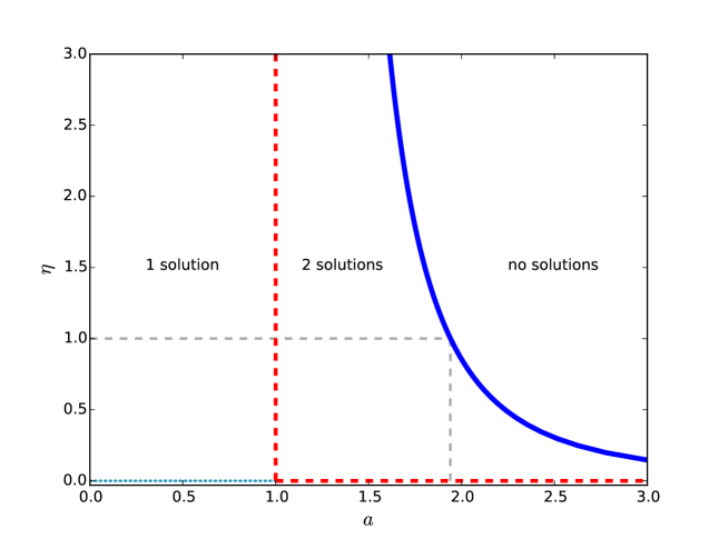
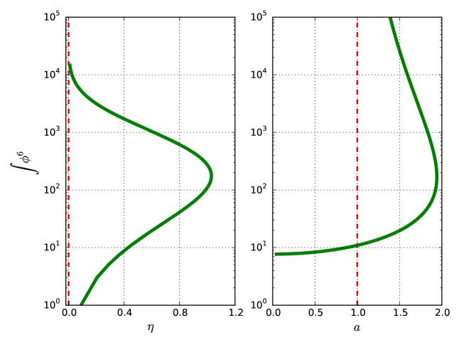
Figure 1. Multiplicity of solutions found on $S^{1}\times T^{2}$. Seed data: $\tau=1+a\cos(s)$ and $\sigma=\eta\hat{\sigma}$. The blue line is a computed fold, whereas the red dashed lines indicate locations where blowup is inferred. The blue dotted line indicates a zero-volume solution, which should be discounted. Solutions along the gray dashed lines are discussed in Figure 2.

Figure 2. Volume of solutions on $S^{1}\times T^{2}$ as the size $\eta$ of the TT tensor (left-hand side) and as the mean curvature $\tau=1+a\cos(s)$ (right-hand side) are varied. The left-hand graph corresponds with the vertical gray dashed line of Figure 2 at $a=1.94$, and right-hand graph corresponds with the horizontal gray dashed line at $\eta=1$.

For solutions $\phi=\phi(s)$ and $W=w(s)\partial_{s}$ of the conformally-parameterized constraint equations (1.4)-(1.5) having the same symmetry as our seed data, the constraint equations reduce to the coupled ODEs

$$-8\varphi^{\prime\prime}+R\varphi+\frac{2}{3}\tau^{2}\varphi^{5} =\frac{2}{3}(\mu+2w^{\prime})^{2}\varphi^{-7}+\eta^{2}\varphi^{-7},$$ (3.2)

$$2w^{\prime\prime} =\tau^{\prime}\varphi^{6},$$ (3.3)

where $R$ is the constant scalar curvature of the product manifold, and where we set $\eta=0$ if $R<0$.

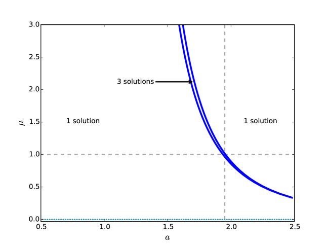
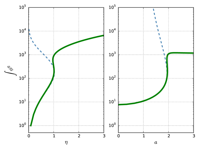
Figure 3. Multiplicity of solutions found on an $S^{1}\times S^{2}$ with $R=0.001$. Here $\tau=1+a\cos(s)$ and $\sigma=\eta\hat{\sigma}$. The blue line is a computed fold. On the blue dotted line at $\mu=0$ (i.e., $\sigma\equiv 0$) there is no solution; the volume has shrunk to zero. Solutions along the gray dashed lines are discussed in Figure 4.

Figure 4. Volume of solutions on an $S^{1}\times S^{2}$ with $R=0.001$ as the size of the TT tensor and as the mean curvature are varied. The left and right-hand graphs correspond with the vertical and horizontal gray dashed lines of Figure 4 respectively. The dashed lines are the corresponding volumes on $S^{1}\times T^{2}$ from Figure 2 for comparison.

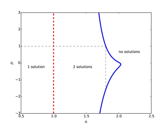
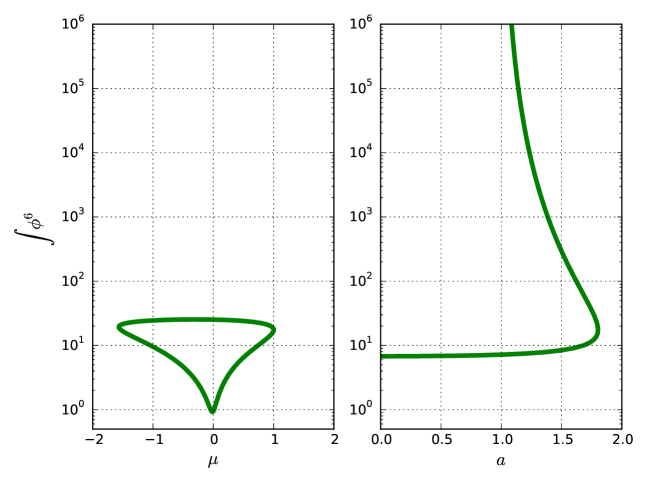
Figure 5. Multiplicity of solutions found on an $S^{1}\times H^{2}$ with negative scalar curvature $R=-0.1$. Seed data: $\tau=1+a\cos(s)$ and $\sigma=\mu\overline{\sigma}$. The blue line is a computed fold, whereas the red dashed line indicate locations where blowup is inferred. Solutions along the gray dashed lines are illustrated in Figure 6.

Figure 6. Volume of solutions on an $S^{1}\times M^{2}$ with $R=-0.1$ as the size of the TT tensor and as the mean curvature are varied. The left and right-hand graphs correspond with the vertical and horizontal gray dashed lines of Figure 6 respectively.

We start by examining solutions on $S^{1}\times T^{2}$, and it turns out that the effects of the two TT tensors $\hat{\sigma}$ (corresponding to the parameter $\eta$) and $\bar{\sigma}$ (corresponding to the parameter $\mu$) are quite different. In particular, if $\eta=0$ and hence $\sigma=\mu\bar{\sigma}$, it is easy to see that $\phi\equiv|\mu|^{1/6}$ and $w=\mu a\sin(s)$ solve system (3.2). These exact solutions are among those discussed in [44], and are the only solutions we were able to find using AUTO. Hence we obtain results consistent with existence and uniqueness for this family, save for the exceptional case $\mu=0$ where the solution degenerates to zero volume.

On the other hand, fixing $\mu=0$, Figure 2 indicates the multiplicity of solutions found on $S^{1}\times T^{2}$ with $\tau=1+a\cos(s)$ and $\sigma=\eta\hat{\sigma}$ as the parameters $a$ and $\eta$ are varied. This computation is an analogue of the examples of [42] recalled in Theorem 1.3, except that it involves a family of smooth, rather than piecewise constant, mean curvatures.

In the region where the mean curvature changes sign, (i.e., for $a>1$) we find a fold, indicated by a solid blue line, and no solutions when the TT tensor is sufficiently large. Figure 2 indicates how the volume of the solution metric changes changes as we traverse the gray dashed lines of Figure 2; the plots, in green, indicate $\int_{S^{1}}\phi^{6}$, which agrees with volume up to an inessential constant factor depending on the second factor of the product manifold. On the vertical gray dashed line, corresponding to Figure 2 (left-hand side), the sign-changing mean curvature is fixed and the size of the TT tensor is varied. When the TT tensor is sufficiently large a fold appears and there are no solutions, and as it is decreased to zero there are two solutions, one heading to zero volume and the other blowing up. The horizontal gray dashed line of Figure 2 corresponds with Figure 2 (right-hand side) and we again observe the fold and a branch where the volume blows up. It is difficult to ascertain from this graph the precise value of $a$ where the blowup occurs, and computationally we found it difficult to approach the singularity. We find, however, that near the singularity the value of $\int\phi^{6}$ along this line is in reasonable agreement with a growth rate $\sim(a-1)^{-5.14}$. In later related examples we find more conclusive evidence of blowup at $a=1$, so we infer this is the case here as well. That is, there is a transition at $a=1$, the threshold of sign-changing mean curvatures. The red dashed lines of Figure 2 indicate locations where we have inferred blowup occurs. The results we observe here are completely parallel with the prior analytical results of [42] found for a more restrictive mean curvature.

Recalling that the only analytical results for sign-changing mean curvatures are available in the Yamabe-null case, we now consider the effect of changing the Yamabe class in these computations. We first consider the Yamabe-positive case by adjusting the previous computation by setting $R=0.001$ in system (3.2) (e.g. by working on an appropriate $S^{1}\times S^{2}$). As in the Yamabe-null setting, when working with families of seed data with $\sigma=\mu\bar{\sigma}$ we found tame behavior (one solution was found for each parameter). On the other hand, for seed data with $\sigma=\mu\hat{\sigma}$ and $\tau=1+a\cos(s)$ the situation is more complicated. Figure 4 indicates the multiplicity of solutions found for this family and can be compared directly with its Yamabe-null counterpart, Figure 2. The region of zero solutions has vanished and we find solutions exist always. However, in a region near the original Yamabe-null fold, we find two folds and a narrow region of multiple solutions in between. Figure 4 shows the effect of traversing along the dashed gray lines of Figure 4 and indicates how the family of solutions in this case corresponds with the Yamabe null families in Figure 2. Note that the various blowup phenomena found in the Yamabe-null case have vanished. The observed fold can be thought of as a purturbation of the situation at $R=0$, and separate computations show that as $R$ is pulled away from zero and approaches, e.g., $R=1$ the volume curves in Figure 4 stablize further, and the doubling back behavior vanishes.

Turning to the Yamabe-negative case we set $R=-0.1$ in equations (3.2) and use $\eta=0$ since we do not have an equivalent for $\hat{\sigma}$ for Yamabe-negative seed data. Thus we use $\mu$ to scale the size of the TT tensor, and unlike the Yamabe-positive and -null cases when using $\sigma=\mu\overline{\sigma}$, we find interesting results; Figure 6 shows the number of solutions found when using mean curvatures of the form $\tau=1+a\cos(s)$. Note that, unlike the parameter $\eta$, system (3.2) does not have even symmetry with respect to $\mu$ and hence our computations involved values of $\mu$ with both signs. As the mean curvature is made increasingly far-from CMC we find a fold, and subsequently no solutions. Just as in the Yamabe-null case, the second branch of solutions blows up at $a=1$, the value of $a$ that transitions from constant-sign to sign-changing mean curvatures; (Figure 6, right-hand side). On the other hand, far enough into the far-from-CMC regime we were unable to find solutions of system 3.2. This is perhaps surprising since in the near-CMC setting one can always find solutions when $\sigma\equiv 0$ (unless $\tau\equiv 0$ as well), and indeed solutions at $\sigma\equiv 0$ are a hallmark of Yamabe-negative CMC seed data. Instead, we find that at $\sigma\equiv 0$, as $a$ is increased to make the solution far-from-CMC, there is a fold around $a=2$ and no solutions were encountered beyond this point. The absence of solutions appears to be loosely associated with the behavior when $\mu=0$ (i.e. $\sigma\equiv 0$), although one notes that the tip of the ‘nose’ on the blue fold line of Figure 6 does not lie on the line $\mu=0$. Therefore, there are values of $a$ where no solutions exist at $\mu\equiv 0$, but for which solutions exist for certain values of $\mu\neq 0$.

3.2. Constant-sign mean curvatures

We now examine excursions into the far-from CMC regime using mean curvatures of the form $\tau=\xi^{a}$, where $\xi$ is a positive function. Starting again with $S^{1}$-dependent data of the form of the previous section, but now with mean curvature $\tau(s)=(\frac{2}{3}-\frac{1}{3}\cos(s))^{a}$, we were only able to find a single solution of the constraint equations for all choices of $a$, $\mu$ and $\eta$, except (as is expected) when $\sigma\equiv 0$ in the Yamabe non-negative case. We can understand the tame behavior we observed by appealing to the limit equation of Theorem 1.2. For $S^{1}$-symmetric solutions of the $S^{1}$-dependent data we consider, the limit equation becomes

$$\left(\frac{W^{\prime}}{N}\right)^{\prime}=\alpha\left|\frac{W^{\prime}}{N}\right|\frac{\tau^{\prime}}{\tau}$$ (3.4)

and it is straightforward to show that this admits no solutions on $S^{1}$.

Theorem 3.1.

Let $\tau>0$ be in $C^{1}$. Then there are no nontrivial $C^{2}$ solutions $W$ of the $S^{1}$-dependent limit equation (3.4).

Proof.

Suppose $W$ is a nontrivial solution, and consider a maximal interval on which $W^{\prime}$ does not vanish. On this interval we have

$$\log(W^{\prime})^{\prime}=k\log(\tau)^{\prime}$$ (3.5)

where $k=\alpha$ if $W^{\prime}>0$ on the interval, and $k=-\alpha$ if $W^{\prime}<0$. Hence

$$W^{\prime}=c\tau^{k}$$ (3.6)

for some constant $c\neq 0$. At the endpoints of the interval $W^{\prime}$ tends to zero. But the right-hand side of equation (3.6) is uniformly bounded away from zero. ∎

Strictly speaking, Theorem 1.2 does not apply in our setting because of the presence of conformal Killing fields. We expect, however, that one can use techniques found in [42] to adapt the main theorem of [17] to this specific family of data to conclude that the nonexistence of solutions to (3.4) implies existence of ($S^{1}$-symmetric) solutions.

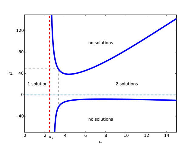
Figure 7. Multiplicity of solutions found on an $S^{2}\times S^{1}$ with positive scalar curvature $R=1$. Seed data: $\tau=(\frac{2}{3}+\frac{1}{3}\cos(\phi))^{a}$ and $\sigma=\mu\overline{\sigma}$. The solid blue line is a computed fold, whereas the red dashed line indicate locations where blowup is inferred. At the dotted blue line at $\mu=0$ there is a zero volume solution which should be discounted. The gray dashed lines are discussed in Figure 8.

Figure 8. Volume of solutions on an $S^{2}\times S^{1}$ with $R=1$ as the size $\mu$ of the TT tensor and as the mean curvature $\xi^{a}$ is varied. The left- and right-hand graphs correspond with the vertical and horizontal gray dashed lines of Figure 8 respectively.

Figure 9. Ratio of $\sqrt{\frac{2}{3}}\varphi^{6}\tau$ to $\left|\frac{1}{2N}\operatorname{\mathcal{L}}W\right|$ as a function of latitude $\phi$ for the large solution of the conformally-parameterized constraint equations at $a=2.46$, $\mu=1$ in Figure 8. The ratio is nearly 1, indicating that the vector field $W$ of the solution is nearly a solution of the limit equation (1.6).

The simple behavior seen for $S^{1}$-dependent data does not hold generally, however. Throughout the remainder of this section we use conformal seed data of the following type:

• The manifold is $S^{2}\times M_{2}$ where $M_{2}$ is one of $S^{1}$,or $H^{2}$. We use $\phi\in(0,\pi)$ for a latitude parameter on $S^{2}$.

• The mean curvature $\tau=\xi^{a}$ depends only on $\phi$, where $0\leq\xi\leq 1$ and $\xi(\phi)=1$ somewhere. In practice we used

  $$\xi(\phi)=\frac{2}{3}-\frac{1}{3}\cos(k\phi)$$

  with $k=1$ or $2$.

• The TT tensor is $\sigma=\mu\overline{\sigma}$, where $\overline{\sigma}$ was introduced in equation (3.1).

• The lapse density is $N=1/2$.

As a first example, consider data on $S^{2}\times S^{1}$. The reduced conformal constraint equations for latitude-dependent data are more complicated than those for $S^{1}$-dependent data; the main differential operators are

$$\operatorname{\Delta}f =\frac{1}{r}\left(f^{\prime\prime}+\cot\phi f^{\prime}\right),\,\,\,\,\,\textrm{ and}$$

$$\mathop{\rm div}\nolimits\mathcal{L}W =(3w^{\prime\prime}+3\cot\phi w^{\prime}+\frac{1}{2r}(1-3\cot^{2}\phi)w)d\phi$$

where $f=f(\phi)$ and $W=w(\phi)d\phi$. We seek solutions of the constrant equations (1.2)-(1.3) the form $\varphi=\varphi(\phi)$ and $W=w(\phi)d\phi$ supplemented with boundary conditions $\varphi^{\prime}=0$ and $w^{\prime}=0$ at $\phi=0$ and $\phi=\pi$ needed to ensure regularity. An additional boundary condition $w=0$ at $\phi=0,\pi$ is effectively enforced by the momentum constraint.

Figure 8 shows the number of solutions found on an $S^{2}\times S^{1}$ with scalar curvature $R=1$ with $\sigma=\mu\overline{\sigma}$ and a relatively simple non-CMC mean curvature

$$\tau=\left[\frac{2}{3}+\frac{1}{2}\cos(\phi)\right]^{a}$$

Theorem 1.5 would apply to this data, except for the usual caveat about conformal Killing fields and, more crucially, the fact that the mean curvature violates the non-generic inequality (1.7). We nevertheless find behaviour consistent with its conclusions: multiple solutions when both $a$ is sufficiently large and $\mu\neq 0$ is sufficiently small. Moreover, the transition to the far-from-CMC regime is abrupt, starting at $a\approx 2.46$, which we will call $a_{*}$. Figure 8, (right-hand side) shows that $a_{*}$ is associated with a blowup of a branch of solutions, and one expects there is a solution of the limit equation (1.6) with $\alpha=1$ at $a=a_{*}$. Indeed, the limit equation arises as the Hamiltonian constraint degenerates to the algebraic equation

$$\sqrt{\frac{2}{3}}\phi^{6}\tau=\left|\frac{1}{2N}\operatorname{\mathcal{L}}W\right|,$$ (3.7)

which can then be substituted back into the momentum constraint. Figure 9 shows the ratio of the two sides of equation (3.7) for the larger of the two solutions at the point $a=2.46$m $\mu=1$ in Figure 8. The ratio is nearly 1, so the solution vector field $W$ at that point is nearly a solution of the limit equation.

The proofs of Theorems 1.4 and 1.5 demonstrate the existence of multiple solutions for $a$ large and $\mu$ small by showing that at $\mu=0$ there is both a zero volume solution and a true solution, and that perturbing off of these yields two solutions; this mechanism is illustrated in Figure 8 (left-hand side). Recall that solutions with $\mu=0$ are impossible in the near-CMC setting for Yamabe-positive seed data such as this, and at the dotted line at $\mu=0$ of Figure 8 there is one less solution than at neighboring points (so there is no solution to the left of the singularity at $a=a_{*}$ and just one solution to the right).

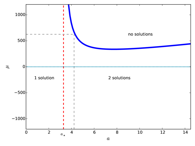
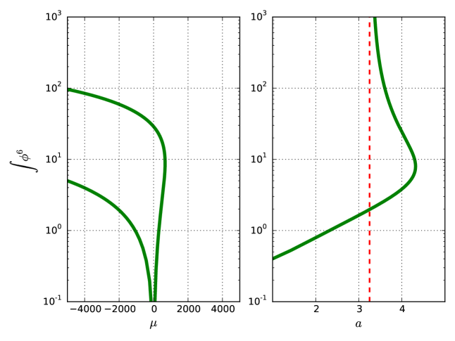
Figure 10. Multiplicity of solutions found on an $S^{2}\times S^{1}$ with positive scalar curvature $R=1$. Seed data: $\tau=(\frac{2}{3}+\frac{1}{3}\cos(2\phi))^{a}$ and $\sigma=\mu\overline{\sigma}$; note the $2$ in the argument of $\cos$. The solid blue line is a computed fold, whereas the red dashed lines indicate locations where blowup is inferred. At the dotted blue line there is a zero-volume solution, which should be discounted. The gray dashed lines are discussed in Figure 11.

Figure 11. Volume of solutions on an $S^{2}\times S^{1}$ with $R=1$ as the size $\mu$ of the TT tensor (left-hand side) and as the mean curvature $\xi^{a}$ (right-hand side) are varied. The left- and right-hand graphs correspond with the vertical and horizontal gray dashed lines of Figure 11 respectively.

As a test of the robustness of these results, consider the same conformal seed data as the previous example, except that the mean curvature is now

$$\tau=\left[\frac{2}{3}+\frac{1}{2}\cos(2\phi)\right]^{a}.$$

Figure 11 illustrates the multiplicity of solutions we found as we varied the parameters $\mu$ and $a$. Here again we find a sharp transition to the far-from-CMC setting, now at $a=a_{*}\approx 3.3$. There is blowup associated with this transition (Figure 11, right-hand side), and again we presume there is a solution to the limit equation with $\alpha=1$ and $a=a_{*}$. For $a>a_{*}$ we find a solution at $\mu=0$ in addition to the zero volume solution (Figure 11, left-hand side), and hence there two solutions for $\mu$ sufficiently small. However, we find an apparent difference between scaling $\mu$ large and positive versus large and negative for this seed data. For $\mu$ positive and large enough (depending on $a$) there are no solutions, just as was the case in Figure 8. But for $\mu$ large and negative we were unable to find a fold and a consequential transition to zero solutions. Instead, the two solutions remain well-separated in volume as $\mu$ is made large (Figure 11, left-hand side). We cannot rule out the possibility that the two branches eventually merge, but this was not the case out to $\mu=-2500000$. Although this data violates inequality 1.7 of Theorem 1.5, our observations are nevertheless consistent with its conclusions. In particular, unlike Theorem 1.4, Theorem 1.5 does not predict non-existence for large TT tensors, and it is conceivable that 1.5 holds more generally for mean curvatures not satisfying inequality 1.7.

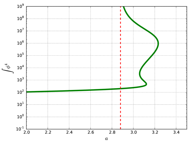
Figure 12. Multiplicity of solutions found on an $S^{2}\times H^{2}$ with positive scalar curvature $R=0.1$. Seed data: $\tau=(\frac{2}{3}+\frac{1}{3}\cos(\phi))^{a}$ and $\sigma=\mu\overline{\sigma}$. The solid blue and purple lines are computed folds, whereas the red dashed line indicate locations where blowup is inferred. At the blue dotted line at $\mu=0$ one solution has zero volume and should be ignored. Solutions along the gray dashed lines are discussed in Figures 13 and 14.

Figure 13. Volume of solutions on an $S^{2}\times H^{2}$ with $R=0.1$ as the mean curvature $\xi^{a}$ (right-hand side) is varied. Solutions correspond with horizontal gray dashed line at $\mu=7$ in Figure 13. At $a=3.1$, four solutions are found for a single conformal seed dataset.

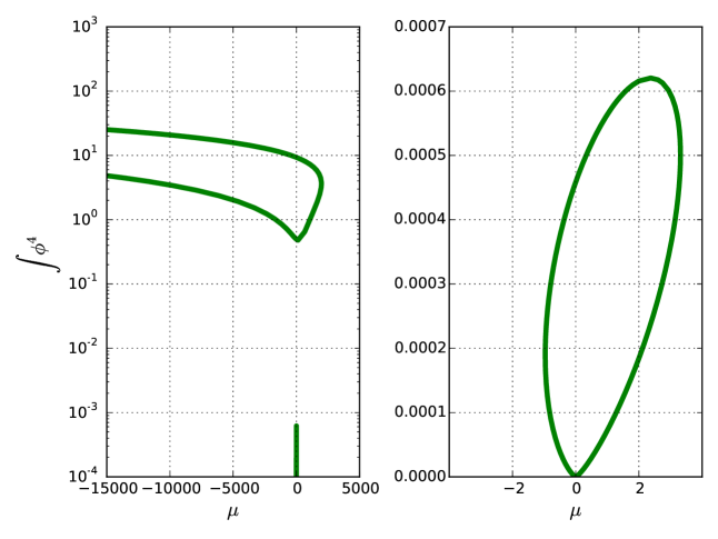
Figure 14. Left-hand side: volume of solutions on an $S^{2}\times H^{2}$ with $R=0.1$ as the size $\mu$ of the TT tensor is varied. Solutions correspond with the vertical gray dashed line at $a=3.2$ in Figure 13. Right-hand side shows a detail of the small loop near $\mu=0$. The large upper loop eventually closes at $\mu\approx-800000$.

The previous two examples involve Yamabe-positive data. To explore the other Yamabe classes we consider latitude-dependent data on $S^{2}\times H^{2}$; by varying the size of the round $S^{2}$ factor we can obtain any desired constant scalar curvature. Before looking at the other Yamabe classes, however, we remark that even for Yamabe-positive data of this type we find differences from what was observed for $S^{2}\times S^{1}$. Figure 13 illustrates the multiplicity of solutions found on an $S^{2}\times H^{2}$ with $R=0.1$, where the seed data has $\sigma=\mu\overline{\sigma}$ and

$$\tau=\left[\frac{2}{3}-\frac{1}{3}\cos(\phi)\right]^{a}.$$

This seed data is comparable to that used for Figure 8, but there are some fine differences in the results. Again we find a sharp transition to the far-from-CMC setting, now at $a=a_{*}\approx 2.8$. However, for $a>a_{*}$ the multiplicity of solutions is a bit complicated. There is a primary fold roughly at $a=3.23$ in the far-from-CMC regime. Beyond this point, the behavior is similar to that of Figure 8, with no solutions when $\mu$ is sufficiently large and two solutions when $\mu\neq 0$ is sufficiently small. Between $a=a_{*}$ and $a=3.23$, however, the situation has changed from that of Figure 8. We found variously between 1 and 4 solutions, and no convincing evidence that there are no solutions when $\mu$ is sufficiently large at, e.g., $a=2.87$.

Figure 13, illustrates how the the various folds appear as the dashed line at $\mu=7$ in Figure 13 is traversed. First the right-most purple fold is encountered, then the left-most and finally the blue fold around $a=3.23$ is hit before heading off to the singularity at $a=a_{*}$. Conversely, Figure 14 illustrates the various solutions along the line $a=3.2$, and we see two disconnected loops (the upper branches in Figure 14, left-hand side, rejoin at $\mu\approx-800000$). As was discussed previously for Figure 8, Figure 14 illustrates how one can visualize the multiple solutions near $\mu=0$ as perturbations of the usual zero solution at $\mu=0$ and the additional three non-trivial solutions we found there.

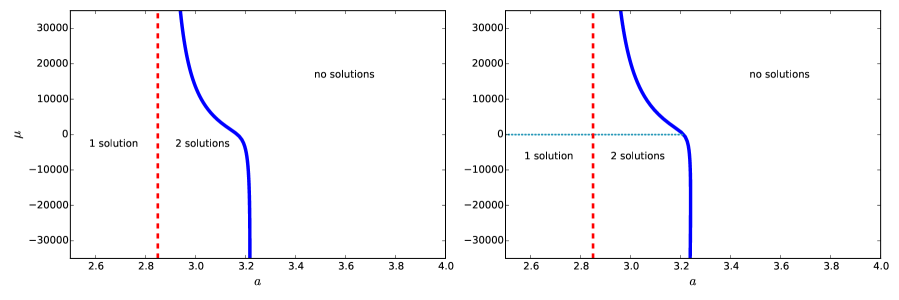
Figure 15. Multiplicity of solutions found on an $S^{2}\times H^{2}$ with scalar curvatures $R=-0.2$ (left-hand side) and $R=0$ (right-hand side). Seed data: $\tau=(\frac{2}{3}-\frac{1}{3}\cos(\phi))^{a}$ and $\sigma=\mu\overline{\sigma}$. The solid blue lines are computed folds, whereas the red dashed lines indicate locations where blowup is inferred. The folds are comparable with the blue fold of Figure 13, which has a similar shape when drawn at this scale. On the right-hand side ($R=0$), the dotted blue line indicates a zero solution which should be discounted. Fine details near $\mu=0$ in the region $2.8<a<3.2$ are potentially unresolved; see Figure 16 (middle).

Turning to non-Yamabe-positive seed data, Figure 15 illustrates the number of solutions found with the same conformal data as in Figure 13, except now with $R=-0.1$ and $R=0$. For this seed data there are no applicable far-from-CMC theorems to guide expectations, and we find a situation similar to the Yamabe-negative sign-changing data of Figure 6. There is a sharp transition to far-from-CMC data at $a_{*}\approx 2.8$, but now solutions vanish sufficiently far into the far-from CMC regime. The blue fold from the Yamabe-positive data of Figure 13 persists, but the purple fold that extended out along the line $\mu=0$ has vanished. The apparent non-existence of solutions far enough into the far-from-CMC regime violates the conclusion of Theorem 1.5, and we therefore suspect that the Yamabe-positive hypothesis of Theorem 1.5 is essential.

Although the vertical scales for Figures 13 and 15 are markedly different, it is not the case that we have missed a fine feature near the line $\mu=0$ in Figure 15 corresponding to the purple folds of Figure 13. Indeed, Figure 16 illustrates the volume of solutions along the line $\mu=0$ (i.e. $\sigma\equiv 0$) for the three cases $R=-0.2$, $R=0$ and $R=0.1$ illustrated in Figures 13 and 15. For far-from-CMC Yamabe-positive seed data (Figure 16, right-hand side) we find solutions at $\sigma\equiv 0$; these solutions are not present for near-CMC data and had not been expected before [45]. By contrast, for the Yamabe-negative seed data the near-CMC solutions at $\sigma\equiv 0$ vanish once the mean curvature is sufficiently far-from CMC (Figure 16, left-hand side). At the boundary $R\equiv 0$ (Figure 16, middle) we find a narrow band in which solutions exist; none in the near-CMC case (which is expected) and none for the far-from CMC seed data as well. The narrow band is reminiscent of the well known one-parameter family of solutions found found for CMC Yamabe-null seed data when $\tau\equiv 0$ and when $\sigma\equiv 0$. It is also similar to the somewhat analogous one-parameter families found for particular Yamabe-null seed data in [42] and [44]. What would have been a vertical line of solutions in the analytic cases has been deformed to the distorted vertical line of Figure 16, middle.

The role of solutions at $\sigma\equiv 0$ appears to be important for understanding the conformal method in the far-from-CMC setting, and we believe this is a consequence of $\sigma$ being absent from the limit equation. Nevertheless, the interplay between $\sigma\equiv 0$ and $\sigma\not\equiv 0$ is nuanced. For example, the breakdown of the existence of solutions along $\sigma\equiv 0$ for Yamabe-negative data (Figure 16, left-hand side) at $a\approx 3.2$ is not perfectly correlated with nonexistence of solutions for nearby values of $a$. This can be seen by inspecting the blue fold of Figure 15, left-hand side. It crosses $\mu=0$ at a value $a\approx 3.2$ but there nevertheless exist certain solutions for values of $a>3.2$ beyond the crossing point, but not much larger.

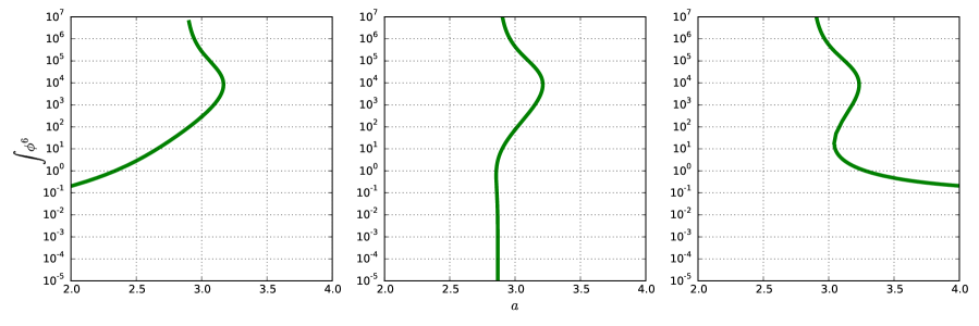
Figure 16. Volume of solutions along $\sigma\equiv 0$ for an $S^{2}\times H^{2}$ having $R=-0.2$ (left), $R=0$ (middle) and $R=0.1$ (right). Mean curvature $\tau=(\frac{2}{3}-\frac{1}{3}\cos(\phi))^{a}$. Conformal seed data is the same as in Figures 13 and 15.

Finally, we consider seed data on $S^{2}\times H^{2}$ with $\sigma=\mu\overline{\sigma}$ and

$$\tau=\left[\frac{2}{3}-\frac{1}{3}\cos(2\phi)\right]^{a},$$

which can be compared with the seed data used for Figure 11. Figure 17 illustrates the number of solutions found for $R=0$ and $R=0.5$, and the outcomes are qualitatively similar to those of Figure 11. In particular, for $\mu<0$ we do not find evidence of non-existence of solutions. On the other hand, for this same data but $R=-1/2$ we obtain multiplicities shown in Figure 18 and find a situation akin to what we have seen previously in Figure 6 and Figure 15 (left-hand side) for Yamabe-negative data: no solutions for $a$ sufficiently large. In an independent computation, not shown, we found that the location of the blue fold crossing $\mu=0$ (e.g. at $a\approx 108$ in Figure 18) grows as $(-R)^{-13}$ and therefore we believe there is indeed a transition at $R=0$ between the two qualitative behaviors seen here for $R=1/2$ and $R=-1/2$.

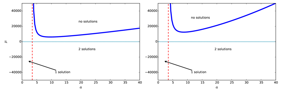
Figure 17. Multiplicity of solutions found on an $S^{2}\times H^{2}$ with scalar curvatures $R=0$ (left-hand side) and $R=0.5$ (right-hand side). Seed data: $\tau=(\frac{2}{3}-\frac{1}{3}\cos(2\phi))^{a}$ and $\sigma=\mu\overline{\sigma}$. The solid blue line indicates a fold, whereas the red dashed line indicate locations where blowup is inferred. The blue dotted lines at $\mu=0$ indicate one solution has zero volume and should be ignored.

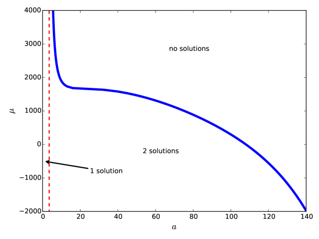
Figure 18. Multiplicity of solutions found on an $S^{2}\times H^{2}$ with scalar curvatures $R=-0.5$ Seed data: $\tau=(\frac{2}{3}-\frac{1}{3}\cos(2\phi))^{a}$ and $\sigma=\mu\overline{\sigma}$. The solid blue indicates a fold, whereas the red dashed line indicate locations where blowup is inferred.

4. Discussion

The limit equation (1.6) appears to play a central role in the solution theory of the conformal method, at least for mean curvatures that do not change sign. In the cases where we could show that there is no solution of the limit equation with the symmetry of the data ($S^{1}$-dependent seed data on $S^{1}\times M_{2}$), we were also unable to find behavior that was any different from the near-CMC theory. For the remaining cases where we investigated constant-sign mean curvatures $\tau=\xi^{a}$, there was a singular value $a_{*}$. For $a>a*$ we found differences from the near-CMC theory: multiple solutions or non-existence of solutions were the general rule, with exceptions occuring only at transitions such as folds. As $a\to a_{*}$ from above, we found solutions of the constraint equations with volumes that appeared to approach infinity; in particular, it was always possible to find such solutions with $\sigma\equiv 0$ We conjecture that at $a=a_{*}$ there is a solution of the limit equation with $\alpha=1$, in which case for each $a>a_{*}$ there is also a solution of the limit equation with $\alpha=a/a_{*}<1$. That is, far-from-CMC behavior appears to occur precisely when a solution to the limit equation exists for some $\alpha\in(0,1]$.

For sign changing mean curvatures, we found a corresponding transition to far-from-CMC phenomena once the mean curvature changed sign. This was certainly true for the Yamabe-negative and Yamabe-null data we examined, and at least weakly so for the Yamabe-positive data of Figure 4 where narrow folds occurred, but unique solutions were more typical. In any event, in these examples, non-standard behaviour only occurred for conformal seed data where the mean curvature changed sign. In may be a that a better parameterization for sign-changing mean curvatures, different from $\tau=1+a\xi$, would provide a sharper, more definitive transition.

Although Theorem 1.1 does not apply, strictly speaking, to our examples (as they possess nontrivial conformal Killing fields), our observations were consistent with it. Whenever we worked with Yamabe-positive seed data we were able to find solutions of the constraint equations, so long as $\sigma\not\equiv 0$ was small enough: Figures 4, 8, 11, 13 and 17 (right-hand side). Conversely, except for cases where we could show that there was not a solution of the limit equation, far-from-CMC Yamabe-negative seed data lead to non-existence sufficiently far into the non-CMC zone: Figures 6, 15 (left-hand side) and 18. This was true even at $\sigma\equiv 0$, in stark contrast to the near-CMC theory.

The situation for Yamabe-null data is harder to characterize. Sometimes it behaved like Yamabe-positive data (Figures 2 and 17, left-hand side), with solutions existing for sufficiently small TT tensors. Sometimes it behaved like Yamabe negative data (Figure 15, right hand side), with solutions vanishing far enough into the far-from CMC zone. Moreover, the analytical work of [42] shows that other variations are also possible.

The conclusions of Theorem 1.5 were found to hold generally, even for mean curvatures that violate inequality 1.7, so long as there appeared to be a solution of the limit equation. That is, for far-from-CMC Yamabe positive data (with constant-sign mean curvature), we found that there were at least two solutions when the TT tensor was small enough (and that there was at least one corresponding nonzero solution at $\sigma\equiv 0$).

On the other hand, Theorem 1.4, which also describes non-existence for Yamabe-positive far-from-CMC seed data when the TT tensor is large, was not found to hold in general. Indeed, we found a hodge-podge of apparent non-existence phenomena on Yamabe-positive seed data. Sometimes there was an immediate onset of nonexistence behavior in the far-from-CMC zone (Figure 8). Sometimes nonexistence was brought on by scaling the TT by a large constant of one sign, but not for large constants of the other sign (Figures 11 and 17 (right-hand side)). In one case (Figure 13) there appeared to be certain far-from-CMC seed data that did not lead to nonexistence regardless of how large the TT tensor was scaled. And in the sign-changing Yamabe-positive case we examined, existence appeared to be pervasive (Figure 4). It is similarly hard to pin down precise non-existence behavior for the Yamabe-null seed data we examined.

We saw no apparent rule to describe the profiles of the various folds we saw. That is, we were unable to discern anything that might help concretely predict the threshold of non-existence when scaling the TT tensor or the specific number of solutions corresponding to given seed data; although zero, one or two solutions were typical, sometimes there were more.

5. Conclusion

Our numerical work suggests that the conformal method appears to suffer from pervasive drawbacks as a parameterization of vacuum, non-CMC solutions of the constraint equations. At least among the data we considered, the general rule was multiple solutions or no solutions at all once the conformal seed data was sufficiently far-from-CMC. Because of the limitations of AUTO, we were only able to examine highly symmetric seed data, and we therefore only probed a select few, very special examples. Nevertheless, it is difficult to imagine that the many cases of multiple solutions we found are not stable under small perturbations of the metric that violate symmetry.

Our results suggest a couple of theorems that might be reasonable targets for future efforts. For example, can non-existence of solutions for sufficiently far-from-CMC Yamabe-negative seed data be established? However, we caution that it is possible that describing the details of the conformal method for far-from-CMC data will lead to a fuller understanding of the conformal method, but also to nothing useful about general relativity. Unless there is some physics associated with to the multiplicity of solutions or the various shapes of the folds, it may simply be that the conformal method is an excellent parameterization of the CMC solutions of the constraints that breaks down as a chart on the larger constraint manifold. Since the conformal method is the only general tool available for constructing solutions of constraint equations de novo, it raises the question of whether a suitable alternative parameterization for non-CMC initial data exists. One potential was proposed in [38] and examined for near-CMC constructions in [25], but its properties in the far-from-CMC setting are unknown and the broader question of finding a well-behaved global parameterization of solutions of the constraint equations is essentally open.

6. Acknowledgments

JD was supported in part by NSF DMS/RTG Award 1345013 and NSF DMS/FRG Award 1262982. MH was supported in part by NSF DMS/FRG Award 1262982 and NSF DMS/CM Award 1620366. TK was supported in part by NSF DMS/RTG Award 1345013. DM was supported in part by NSF DMS/FRG Award 1263544.

Appendix A A constant norm TT tensor on $S^{1}\times S^{2}$

In this section we construct a transverse-traceless tensor on $S^{1}\times S^{2}$ that has constant norm and is pointwise orthogonal to $\operatorname{\mathcal{L}}W$ when $W$ is an $S^{1}$-dependent vector field pointing along $S^{1}$.

Consider normal (polar) coordinates $(r,\theta)$ on the unit round sphere $S^{2}$ centered at the north pole, so that the metric has the form $g=dr^{2}+\sin^{2}(r)d\theta^{2}$. Let $\omega=\sin(r)d\theta$. It is clear that $\omega$ fails to be continuous at the north and south poles of $S^{2}$, but is otherwise smooth. A straightforward computation shows that $|\nabla\omega|=\cot(r)$. The singularity at $r=0$ is $O(r^{-1})$, with similar remarks holding at $r=\pi$. Hence $\omega\in W^{1,p}(S^{2})$ for any $p<2$. Moreover, $\mathop{\rm div}\nolimits\omega=0$ in the region where $\omega$ is smooth (i.e. almost everywhere) and therefore $\omega$ is weakly divergence free.

Now let $s$ denote a unit speed parameter on $S^{1}$ and set

$$\hat{\sigma}=\omega\otimes ds+ds\otimes\omega$$

on $S^{1}\times S^{2}$. Clearly $\sigma$ is trace-free. Moreover since $\omega$ and $ds$ are both divergence free, $\sigma$ is a transverse-traceless tensor on $S^{1}\times S^{2}$. Finally,

$$|\sigma|^{2}=2\left|\omega\right|^{2}\left|dz\right|^{2}+4\left<\omega,dz\right>=2\left|\omega\right|^{2}=2\sin^{2}(r)\left|d\theta\right|^{2}=2\sin^{2}(r)(\sin(r))^{-2}=2,$$

except at $r=0$ and $r=\pi$. That is, $\left|\sigma\right|^{2}=2$ almost everywhere. Hence $\hat{\sigma}$ is a constant-norm $W^{1,p}$ transverse-traceless tensor on $S^{1}\times S^{2}$ for any $p<2$. Although this level of regularity is not ideal, it falls within the a category of regularity easily handled for the conformal method (e.g. [8]).

If $W=w(s)\partial_{s}$ then $\operatorname{\mathcal{L}}W=2w^{\prime}(\frac{2}{3}ds\otimes ds-\frac{1}{3}g^{\circ}$), where $g^{\circ}$ is the round metric on the sphere. Since $\hat{\sigma}$ only has $ds\otimes d\theta$ and $d\theta\otimes ds$ components, it is pointwise orthogonal to any such $\operatorname{\mathcal{L}}W$.

References

- [1] P. T. Allen, A. Clausen, and J. Isenberg. Near-constant mean curvature solutions of the Einstein constraint equations with non-negative Yamabe metrics. Classical and Quantum Gravity, 25(7):075009, 2008.
- [2] L. Andersson and P. T. Chruściel. Solutions of the constraint equations in general relativity satisfying “hyperboloidal boundary conditions”, volume 355 of Dissertationes Math.(Rozprawy Mat.). Polska Akademia Nauk, Instytut Matematyczn, 100 edition, 1996.
- [3] R. Bartnik and J. Isenberg. The constraint equations. In The Einstein equations and the large scale behavior of gravitational fields, pages 1–38. Birkhäuser, Basel, 2004.
- [4] A. Behzadan and M. Holst. Rough solutions of the Einstein constraint equations on asymptotically flat manifolds without near-CMC conditions. Submitted for publication. Available as arXiv:1504.04661 [gr-qc].
- [5] D. Bernstein and M. Holst. A 3D finite element solver for the initial-value problem. In A. Olinto, J. A. Frieman, and D. N. Schramm, editors, Proceedings of the Eighteenth Texas Symposium on Relativistic Astrophysics and Cosmology, December 16-20, 1996, Chicago, Illinois, Singapore, 1998. World Scientific.
- [6] A. Champneys, Y. Kuznetsov, and B. Sandstede. A numerical toolbox for homoclinic bifurcation analysis. International Journal of Bifurcation and Chaos, 6:867–887, 1996.
- [7] Y. Choquet-Bruhat. Einstein constraints on compact n-dimensional manifolds. Class. Quantum Grav., 21:S127–S151, 2004.
- [8] Y. Choquet-Bruhat. Einstein constraints on compact -dimensional manifolds. Classical Quantum Gravity, 21(3):S127–S151, 2004. A spacetime safari: essays in honour of Vincent Moncrief.
- [9] Y. Choquet-Bruhat, J. Isenberg, and J. W. York, Jr. Einstein constraints on asymptotically Euclidean manifolds. Phys. Rev. D (3), 61(8):084034, 20, 2000.
- [10] S. Chow and J. Hale. Methods of Bifurcation Theory. Springer-Verlag New York Inc., New York, 1982.
- [11] P. Chrusciel and R. Gicquaud. Bifurcating solutions of the Lichnerowicz equation. Annales Henri Poincaré, 18(2):643–679, 2017.
- [12] P. T. Chruściel and R. Mazzeo. Initial data sets with ends of cylindrical type: I. the Lichnerowicz equation. Annales Henri Poincaré, 16(5):1231–1266, 2015.
- [13] P. T. Chruściel, R. Mazzeo, and S. Pocchiola. Initial data sets with ends of cylindrical type: II. the vector constraint equation. Advances in Theoretical and Mathematical Physics, 17:829–865, 2013. arXiv:1203.5138v1 [gr-qc].
- [14] G. Cook and S. Teukolsky. Numerical relativity: Challenges for computational science. In A. Iserles, editor, Acta Numerica 8, pages 1–44. Cambridge University Press, 1999.
- [15] G. B. Cook. Initial data for axisymmetric black-hole collisions. Phys. Rev. D, 44(10):2983–3000, 1991.
- [16] G. B. Cook. Initial data for numerical relativity. Liv. Rev. Relativ., 3:5, 2000.
- [17] M. Dahl, R. Gicquaud, and E. Humbert. A limit equation associated to the solvability of the vacuum Einstein constraint equations using the conformal method. Duke Math. J., 161(14):2669–2697, 2012.
- [18] S. Dain. Trapped surfaces as boundaries for the constraint equations. Class. Quantum Grav., 21(2):555–573, 2004.
- [19] J. Dilts. The Einstein Constraint Equations on Compact Manifolds with Boundary. Class. Quant. Grav., 31:125009, 2014.
- [20] J. Dilts, J. Isenberg, R. Mazzeo, and C. Meier. Non-CMC solutions of the Einstein constraint equations on asymptotically euclidean manifolds. Class. Quantum Grav., 31:065001, 2014.
- [21] R. Gicquaud and C. Huneau. Limit equation for vacuum einstein constraints with a translational killing vector field in the compact hyperbolic case. Journal of Geometry and Physics, 107:175 – 186, 2016.
- [22] R. Gicquaud and Q.-A. Ngo. A new point of view on the solutions to the Einstein constraint equations with arbitrary mean curvature and small TT-tensor. Class. Quantum Grav., 31(19):1–16, 2014.
- [23] R. Gicquaud and A. Sakovich. A large class of non constant mean curvature solutions of the Einstein constraint equations on an asymptotically hyperbolic manifold. Communications in Mathematical Physics, 310(3):705–763, 2012.
- [24] M. Holst. Adaptive numerical treatment of elliptic systems on manifolds. Adv. Comput. Math., 15(1–4):139–191, 2001.
- [25] M. Holst, D. Maxwell, and R. Mazzeo. Conformal fields and the structure of the space of solutions of the Einstein constraint equations. arXiv:1711.01042.
- [26] M. Holst and C. Meier. Non-uniqueness of solutions to the conformal formulation. Accepted for publication in Annales Henri Poincaré. Available as arXiv:1210.2156 [gr-qc].
- [27] M. Holst and C. Meier. Non-CMC solutions of the Einstein constraint equations on asymptotically Euclidean manifolds with apparent horizon boundaries. Class. Quantum Grav., 32(2):1–25, 2014.
- [28] M. Holst, C. Meier, and G. Tsogtgerel. Non-CMC solutions of the Einstein constraint equations on compact manifolds with apparent horizon boundaries. 2018.
- [29] M. Holst, G. Nagy, and G. Tsogtgerel. Rough solutions of the Einstein constraints on closed manifolds without near-CMC conditions. Comm. Math. Phys., 288(2):547–613, 2009.
- [30] M. Holst and G. Tsogtgerel. The Lichnerowicz equation on compact manifolds with boundary. Class. Quantum Grav., 30(20):1–31, 2013.
- [31] J. Isenberg. Constant mean curvature solutions of the Einstein constraint equations on closed manifolds. Classical Quantum Gravity, 12(9):2249–2274, 1995.
- [32] J. Isenberg and V. Moncrief. A set of nonconstant mean curvature solutions of the Einstein constraint equations on closed manifolds. Classical Quantum Gravity, 13:1819–1847, 1996.
- [33] J. Isenberg and N. Ó Murchadha. Non-CMC conformal data sets which do not produce solutions of the Einstein constraint equations. Classical Quantum Gravity, 21:S233, 2004.
- [34] J. Isenberg and J. Park. Asymptotically hyperbolic non constant mean curvature solutions of the Einstein constraint equations. Classical and Quantum Gravity, 14:A189–A202, 1997.
- [35] H. B. Keller. Numerical Methods in Bifurcation Problems. Tata Institute of Fundamental Research, Bombay, India, 1987.
- [36] H. Kielhöfer. Bifurcation theory, volume 156 of Applied Mathematical Sciences. Springer-Verlag, New York, 2004. An introduction with applications to PDEs.
- [37] A. Lichernowicz. Sur l’intégration des équations d’Einstein. J. Math. Pures Appl., 23:26–63, 1944.
- [38] D. Maxwell. Initial data in general relativity described by expansion, conformal deformation and drift. To appear, Comm. Anal. Geom. Available as arXiv:1407.1467 [gr-qc].
- [39] D. Maxwell. Solutions of the Einstein constraint equations with apparent horizon boundaries. Comm. Math. Phys., 253(3):561–583, 2005.
- [40] D. Maxwell. Rough solutions of the Einstein constraint equations. J. Reine Angew. Math., 590:1–29, 2006.
- [41] D. Maxwell. A class of solutions of the vacuum Einstein constraint equations with freely specified mean curvature. Math. Res. Lett., 16(4):627–645, 2009.
- [42] D. Maxwell. A model problem for conformal parameterizations of the Einstein constraint equations. Communications in Mathematical Physics, 302:697–736, 2011. 10.1007/s00220-011-1187-z.
- [43] D. Maxwell. The conformal method and the conformal thin-sandwich method are the same. Classical and Quantum Gravity, 31(14):145006, 2014.
- [44] D. Maxwell. Conformal parameterizations of slices of flat Kasner spacetimes. Annales Henri Poincaré, pages 1–36, 2014.
- [45] T.-C. Nguyen. Nonexistence and nonuniqueness results for solutions to the vacuum Einstein conformal constraint equations. Available as arXiv:1507.01081 [math.AP].
- [46] T.-C. Nguyen. Progress on nonuniqueness of solutions to the vacuum Einstein conformal constraint equations with positive Yamabe invariants. arXiv:1802.00077.
- [47] N. O’Murchadha and J. York, Jr. Existence and uniqueness of solutions of the Hamiltonian constraint of general relativity on compact manifolds. J. Math. Phys., 14(11):1551–1557, 1973.
- [48] H. Pfeiffer. The initial value problem in numerical relativity. In Proceedings of the Miami Waves 2004 Conference, 2004.
- [49] J. W. York, Jr. Conformally invariant orthogonal decomposition of symmetric tensors on Riemannian manifolds and the initial-value problem of general relativity. J. Math. Phys., 14:456–464, 1973.
- [50] J. W. York, Jr. Conformal “thin-sandwich” data for the initial-value problem of general relativity. Phys. Rev. Lett., 82(7):1350–1353, 1999.
- [51] E. Zeidler. Nonlinear functional analysis and its applications. I. Springer-Verlag, New York, 1986. Fixed-point theorems, Translated from the German by Peter R. Wadsack.
- [52] E. Zeidler. Nonlinear Functional Analysis and its Applications, volume I: Fixed Point Theorems. Springer-Verlag, New York, NY, 1991.