11email: [uklein]@astro.uni-bonn.de 22institutetext: Departamento de Física Teórica y del Cosmos, Universidad de Granada, Spain
22email: [ute,simon]@ugr.es 33institutetext: Instituto Universitario Carlos I de Física Teórica y Computacional, Facultad de Ciencias, 18071 Granada, Spain
Radio synchrotron spectra of star-forming galaxies
The radio continuum spectra of 14 star-forming galaxies are investigated by fitting nonthermal (synchrotron) and thermal (free-free) radiation laws. The underlying radio continuum measurements cover a frequency range of 325 MHz to 24.5 GHz (32 GHz in case of M 82). It turns out that most of these synchrotron spectra are not simple power-laws, but are best represented by a low-frequency spectrum with a mean slope (), and by a break or an exponential decline in the frequency range of 1 – 12 GHz. Simple power-laws or mildly curved synchrotron spectra lead to unrealistically low thermal flux densities, and/or to strong deviations from the expected optically thin free-free spectra with slope in the fits. The break or cutoff energies are in the range of 1.5 - 7 GeV. We briefly discuss the possible origin of such a cutoff or break. If the low-frequency spectra obtained here reflect the injection spectrum of cosmic-ray electrons, they comply with the mean spectral index of Galactic supernova remnants. A comparison of the fitted thermal flux densities with the (foreground-corrected) H fluxes yields the extinction, which increases with metallicity. The fraction of thermal emission is higher than believed hitherto, especially at high frequencies, and is highest in the dwarf galaxies of our sample, which we interpret in terms of a lack of containment in these low-mass systems, or a time effect caused by a very young starburst.
Key Words.:
galaxies: radio continuum, star formation, magnetic fields; radiation mechanisms: non-thermal, thermal1 Introduction
Star-forming galaxies emit both thermal (free-free) and nonthermal (synchrotron) radiation in the radio regime. It is known since a few decades that the synchrotron component dominates at frequencies up to about 10 GHz (Klein & Emerson 1981; Gioia et al. 1982) and that the overall slope of the observed spectra has a mean value of about 0.70 to 0.75, with little dispersion (about 0.10). And for decades, the perception has been that the spectra are the superposition of two power-laws,
| (1) |
where is the spectral index of the synchrotron radiation spectrum. The superposition of thermal and synchrotron radiation thus produces a flattening of the total radio spectrum towards high frequencies, with the asymptotic value of . This, however, can hardly be seen, owing to the onset of thermal radiation from dust, which becomes significant above about 40 GHz.
In the past decade, numerous studies have been dedicated to characterize the shape of the radio spectrum. The two major questions have been: What is the contribution of the thermal emission (thermal fraction, )? What is the synchrotron spectral index, , and how does it change with frequency? Past studies have given different answers, owing to the differences in the covered frequency range and the sample selection. Gioia et al. (1982) found a mean spectral index of the total radio continuum emission of , based on a sample of 56 galaxies, which they had observed at 408 MHz, 4.75 and 10.7 GHz. They concluded that the spectral index of the synchrotron radiation is , with the synchrotron emission dominating below 10 GHz. They estimated the fraction of thermal radiation to be . Klein (1988) found a mean value of , and a fraction of thermal emission of % at 10 GHz. Duric et al. (1988), however, claimed a large variation of the thermal fraction in a sample of 41 spiral galaxies. Niklas et al. (1997) found a thermal fraction , based upon observations of a sample of 74 Shapley-Ames galaxies at 10.7 GHz. Williams & Bower (2010) obtained radio continuum spectra of galaxies with continuous frequency coverage between 1 and 7 GHz. They found curved synchrotron spectra for the starburst galaxies NGC 253, M 82, and Arp 220. Marvil et al. (2015) presented radio continuum spectra of 250 bright galaxies, reporting a curvature of the spectra between 74 MHz and 4.85 GHz, with changing from 0.45 to 0.69. These latter two papers strongly indicate that the synchrotron spectra of star-forming galaxies cannot be simple power-laws, but probably decline with increasing frequency in the cm-wavelength range. Recently, Tabatabaei et al. (2017) presented measurements of 61 galaxies 1.4, 4.8, 8.5, and 10.5 GHz. Their analysis delivered a total spectral index of , a mean synchrotron spectral index of , and a fraction of thermal radiation of .
There are several reasons that may have led to the variety of the derived synchrotron spectra and thermal fractions summarized above, some of which are contradicting. First, the quality of early ( 1990) continuum measurements of galaxies has been inferior to that of observations conducted thereafter. Second, the sample sizes used in the analyses were rather different, and the frequency coverage of the measurements culled from the literature too small. Third, the careful data selection described in Sect.3 may not have been made in some of the works.
The spectrum of the diffuse synchrotron emission is shaped by the processes that characterize the propagation of relativistic electrons, in particular the type of propagation (diffusion or convection), of energy losses (synchrotron, inverse-Compton, adiabatic losses or bremsstrahlung), and the confinement to the galaxy. It is generally accepted that the acceleration takes place in the shocks of supernova remnants (SNRs), which have an average spectral index of -0.5 Green (2014). From there, the relativistic particles propagate into the interstellar medium (ISM) via diffusion and/or convection, and lose energy. The dominant energy losses at high frequencies are synchrotron and inverse-Compton losses, which steepen the synchrotron spectrum. At low frequencies thermal absorption would flatten the spectra and may even produce a turn-over at the lowest frequencies (see the papers and discussion by Israel & Mahoney 1990; Hummel 1991). However, for the frequency range considered in the present paper, we are not concerned with this latter process, as it would require extreme emission measures in order to become relevant for the frequency range considered here.
In this paper, we present an analysis of accurately determined radio continuum spectra of 14 star-forming galaxies, comprising massive grand-design, closely interacting, and low-mass (dwarf) galaxies. The spectra cover a frequency range 325 MHz – 24.5 GHz (32 GHz in case of M 82), with the 24.5 GHz measurements performed with the Effelsberg 100-m telescope in the mid 80’s, and mostly unpublished to date. All other flux densities were carefully selected from the literature. For the first time, the data allow a reliable separation of the thermal and nonthermal components to be performed, hence an analysis of the resulting synchrotron spectra, and a firm extrapolation towards lower frequencies. This kind of work is also considered valuable towards establishing and interpreting low-frequency spectra of galaxies obtained with LOFAR observations (see, e.g., Mulcahy et al. 2014). However, for this paper we decided not to use measurements at frequencies below 325 MHz, since astrophysical processes that shape the spectra there would increase the number of free parameters unnecessarily.
In Sect. 2 we present the galaxy sample and their selection criteria. The data selection made for the present investigation is described in Sect. 3. In Sect. 4 the fitting procedure of the spectra is described, and in Sect. 5 the results are presented. These are discussed in Sect. 6, while Sect. 7 contains a summary and lists our conclusions.
2 The Galaxies
The galaxy sample used for our analysis was determined by the inclusion of high-frequency radio continuum data (see Sect. 3.2), which are avaliable for a small number of galaxies mapped with the Effelsberg 100-m telescope years ago. This results in a mixture of rather different galaxy types, spanning the whole mass range of star-forming galaxies and incorporating closely interacting pairs and ongoing mergers. These galaxies have very high star formation rates per unit surface, hence all of them are rather radio-bright. In what follows we shall briefly introduce the galaxies and their pertinent properties, subdividing them into several categories. All subsequent tables of this paper follow this categorization using dashed horizontal lines.
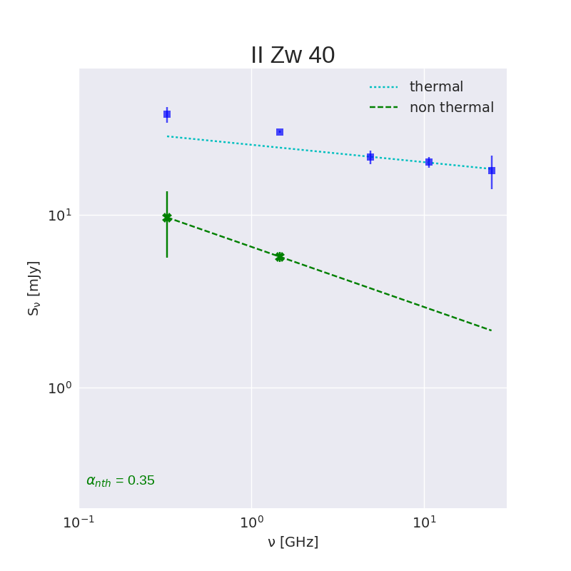
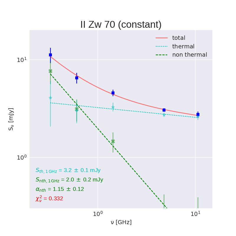
Dwarf galaxies: There are five low-mass galaxies in our sample. II Zw 40 and II Zw 70 are classical blue compact dwarf galaxies (BCGDs). BCDGs are also called H ii galaxies because they are dominated by giant H ii regions occupying much of their total volumes. Their emission-line spectra indicate that they are metal-poor, while they are gas-rich and are experiencing intense bursts of star formation. II Zw 40 was observed in the radio continuum by Klein et al. (1984b), Klein et al. (1991), and by Deeg et al. (1993). II Zw 70 is a small and distant BCDG so that existing radio continuum measurements by (Klein et al. 1984b; Skillman & Klein 1988; Deeg et al. 1993) only provided integrated flux densities. The high-frequency radiation of these two galaxies is purely thermal.
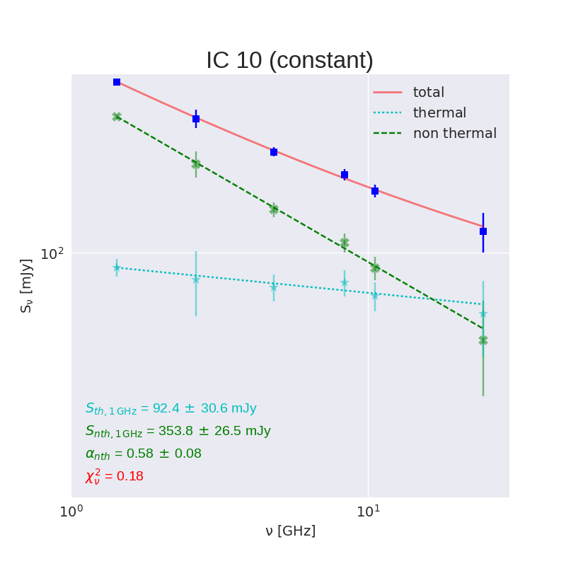
IC 10, NGC 1569, and NGC 4449 are nearby starbursting dwarf galaxies. They have properties that are rather similar to those of BCDGs. They are gas-rich, too, but their metallicities are not so low.
Because of its proximity to the Galactic plane, IC 10 is a tricky case for radio continuum observations. In particular at low frequencies, at which interferometric observations are indispensable, imaging suffers from contamination by spurious sidelobes from radio continuum structures in the Galactic plane. Another worry is thermal absorption through the plane at the lowest frequencies. Useful measurements for our purpose have been carried out Klein et al. (1983), Klein & Gräve (1986), Chyży et al. (2003), and by Chyży et al. (2016).
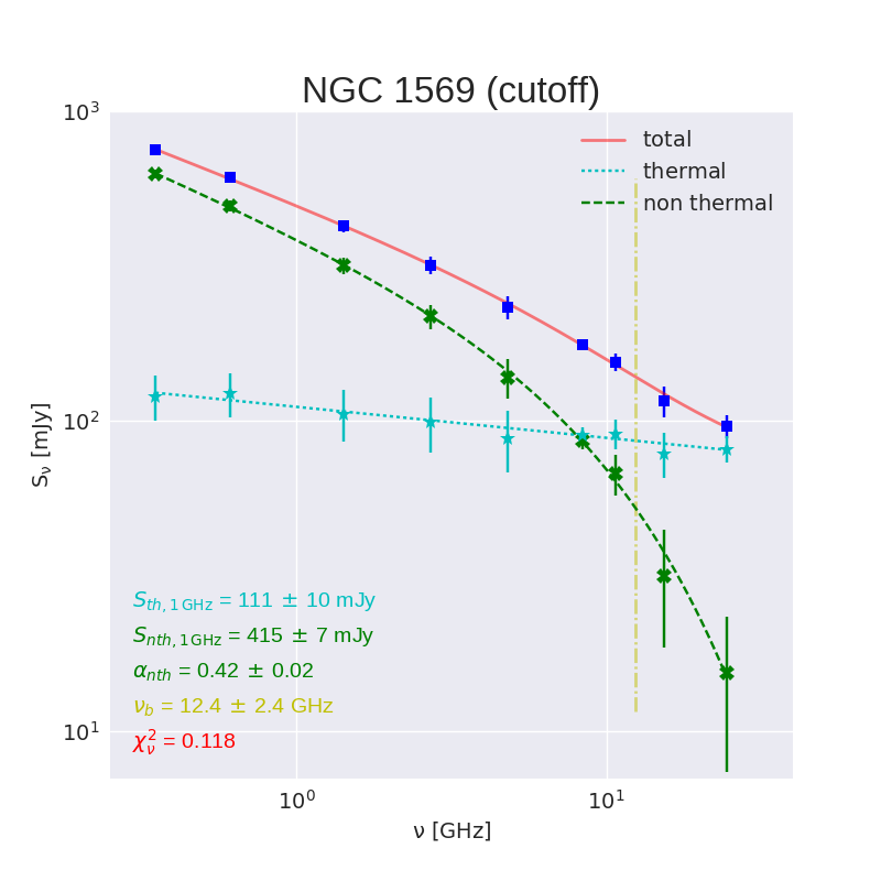
NGC 1569 is considered as a template of a low-mass galaxy with an evolved starburst. Israel & de Bruyn (1988) were the first to notice that the synchrotron spectrum is not a simple power-law, but ‘has a high-frequency cutoff at GHz’. This rapid decline is not obvious in the total radio spectrum, due to a high fraction of thermal radio emission, which was derived by Israel & de Bruyn (1988) from the H emission. Numerous radio continuum studies at a multitude of frequencies, which aimed at an understanding of cosmic-ray propagation into the halo regime of this dwarf galaxy (Klein & Gräve 1986; Lisenfeld et al. 2004; Kepley et al. 2010; Purkayastha 2014) prove its intense star formation. It is among the radio-brightest in our sample and possesses a low-frequency radio halo.
Another such nearby template of a starburst dwarf galaxy, NGC 4449, has been observed in the radio continuum by Klein & Gräve (1986, 24.5 GHz), Chyży et al. (2000, 4.9, 8.5 GHz), Chyży et al. (2011, 2.7, 4.9 GHz), Srivastava et al. (2014, 150, 325, 610 MHz), and by Purkayastha (2014, 350 MHz). This galaxy, too, is characterized by a high star formation rate (SFR), which was most likely triggered by the close passage of another - yet lower-mass - galaxy. NGC 4449 also possesses a low-frequency radio halo.
Interacting galaxies: Upon close inspection, almost all galaxies are gravitationally interacting with another to some extent. In the present sample, NGC 4490/85, NGC 5194/95 (M 51), and NGC 4631 (with nearby dwarf elliptical NGC 4627 and the more massive disk galaxy NGC 4652) have nearby and obviously interacting companion galaxies. These interactions are the likely cause of the intense ongoing star formation in these galaxies, with the close companions stirring up the gas and giving rise to gas compression and subsequent star formation out of the molecular gas.
Radio continuum studies of NGC 4490/85, a closely interacting pair of galaxies, were reported by Viallefond et al. (1980, 1.4 GHz), Clemens et al. (1999, 1.49, 4.86, 8.44, 15.2 GHz), and by Klein et al. (1983, 24.5 GHz). Nikiel-Wroczyński et al. (2016) published a multi-frequency radio continuum study of this system using archival VLA data and new GMRT observations at 610 MHz. The highest frequency at which NGC 4490/85 has been studied was 25 GHz (Klein 1983).
M 51 has been the target of numerous radio continuum studies, which in the early days aimed at measuring the total radio continuum spectrum and studying cosmic-ray propagation (Klein et al. 1984a), and later on focused on investigating the structure of the large-scale magnetic field in it (e.g. Neininger 1992; Fletcher et al. 2011; Mao et al. 2015). The rich set of flux-density measurements available for this galaxy required a careful selection, with only the most reliable data in terms of confusion and missing short spacings culled by us. Klein et al. (1984a) inferred a simple power-law for the synchrotron spectrum of M 51.
After the discovery of an extended radio continuum halo at 610 and 1412 MHz around NGC 4631 by Ekers & Sancisi (1977) there has been a large number of observations at higher frequencies (Hummel & Dettmar 1990a; Hummel et al. 1991; Golla 1999; Irwin et al. 2012). These mostly aimed at studying cosmic-ray transport out of the disk and at investigating the morphology of the magnetic field of this galaxy. The high star-formation rate is probably caused by the gravitational interaction with the neighbouring galaxies NGC 4627 and NGC 4652, rendering this galaxy a rather radio-bright one.
Merging galaxies: In case of ongoing mergers, star formation is extreme, owing to the collision of molecular clouds in the merging centres of the two galaxies.
NGC 4038/39, the ‘Antenna Galaxy’, represents one of the classical nearby ongoing mergers of two galaxies. Chyży & Beck (2004a) and Basu et al. (2017) performed thorough radio continuum studies, with the emphasis on the linear polarization and on the resulting morphology of the large-scale magnetic field in NGC 4038/39. In separating the thermal from the nonthermal radio emission, they inferred a simple power-law for the total synchrotron spectrum of this system.
NGC 6052, which became known as a so-called ‘clumpy irregular galaxy’ under its label Mkn 297 (Heidmann 1979), is revealed as a close merger of two galaxies oriented perpendicularly by HST images (Holtzman et al. 1996). It has a high radio brightness. High-resolution radio continuum observations of this system were reported by Deeg et al. (1993).
Starburst galaxies: NGC 2146 and NGC 3034 (M 82) are classical nearby starburst galaxies, again with the intense star-forming activity resulting from gravitational interaction with a nearby galaxy or from a past merger event. A comprehensive radio continuum study of NGC 2146 was reported by Lisenfeld et al. (1996), who investigated the cosmic-ray transport in this galaxy. NGC 3034 (M82) has been the target of a large number of radio continuum studies across a large frequency range. Adebahr et al. (2013) presented observations at 3, 6, 22, and 92 cm, using the VLA and the WSRT. Varenius et al. (2015) made dedicated measurements with LOFAR to image the radio continuum of M 82 at 118 and 154 MHz. However, such low-frequency measurements are not relevant for our present study, since at frequencies below about 1 GHz various effects may shape the synchrotron spectra in such a way as to produce deviations from a simple power-law (see Sect. 3.2). Klein et al. (1988) published observations of M 82 at 32 GHz, the highest frequency at which thermal radiation from dust is still insignificant.
NGC 3079 and NGC 3310 are starburst which can be considered as transition phases towards AGN (active galactic nucleus) activity. NGC 3079 exhibits a focused wind emerging from its centre and giving rise to a ‘figure-8’ bow-shock structure seen in the nonthermal radio continuum (Duric et al. 1983; Duric & Seaquist 1988). NGC 3310 has recently swallowed one of its dwarf companion galaxies (see, e.g., Kregel & Sancisi 2001), this having led to the enormous starburst. High-resolution radio continuum observations were performed by Duric et al. (1986), with the aim to study the distribution of cosmic rays in this galaxy.
3 The data
3.1 24.5 GHz measurements
The observations at 24.5 GHz had been performed in perfect weather during test measurements in February 1982. The K-band maser receiver system with a bandwidth 100 MHz had been installed in the primary focus of the Effelsberg 100-m telescope. The half power beam width (HPBW) was measured to be 38′′ 1′′. The frontend was equipped with two horns, giving an angular beam separation of 114′′ 2′′ on the sky. The aperture efficiency of the 100-m telescope was 19% at the time of the observations. The pointing and focus of the telescope were checked using the point source 3C 286, with small maps centered on this source providing also the flux calibration. The flux density scale is that of Baars et al. (1977). For each galaxy, six coverages were taken between 50∘ and 80∘ elevation (corresponding to system temperatures of 79 K and 49 K, respectively, on the sky), using a scan separation of 10′′. These were stacked to yield final maps with an root mean square (rms) noise of 2.9 mJy/beam area. The observing procedure and reduction technique is essentially the same as described by Emerson et al. (1979). The sample selection was governed by the radio brightness and sizes of the target galaxies, dictated by the rather high frequency and the comparatively small bandwidth of the maser receiver. Since those were the first (and only) measurements of this kind, it was attempted to include star-forming galaxies with a variety of properties (low- and high-mass galaxies, interacting systems).
3.2 Literature search
In what follows we describe the compilation of the data used below 24.5 GHz. All published flux densities used here were checked for the calibration scale and, wherever necessary, were scaled to the common scale of Baars et al. (1977). At the highest frequencies (24.5 and 32 GHz), the Baars scale is higher than that properly extended to higher frequencies by Perley & Butler (2013). This small diifference does not affect our analysis.
A careful selection was made to ensure that the most reliable data would be used. We discarded interferometric measurements that might underestimate the flux density as a result of missing short spacings (mostly relevant above about 1.4 GHz), but also single-dish measurements that might overestimate the flux density owing to source confusion (mostly relevant below about 5 GHz). If several measurements are available at the same or a neighbouring frequency, we calculated the error-weighted average at the corresponding mean frequency. The resulting data compilation is presented in tabular form in App. A. For each galaxy, the tables give the mean frequency in GHz (Col. 1), the flux density (Col. 2) and its error (Col. 3) in mJy, and the reference to the flux density measurement (Col. 4). In a few cases, we have determined flux densities at 325 MHz and 1.4 GHz using the Westerbork Northern Sky Survey (WENSS) (Rengelink et al. 1997) and the NRAO VLA Sky Survey (NVSS) (Condon et al. 1998), respectively. These are galaxies with small angular sizes so that flux loss by interfreometric measurements is not an issue. Finally, some flux densities were recently obtained in the course of other observing programmes (VLA, Effelsberg).
We decided to utilize only flux densities above 0.3 GHz, since at lower frequencies a number of astrophysical effects such as thermal absorption may shape the synchrotron spectra in such a way as to produce deviations from a simple power-law. It would require more free parameters, rendering the fit results less reliable when taking these processes into account. The synchrotron spectra obtained here may serve though to extrapolate them to lower frequencies and thus provide a firm ‘leverage’ for low-frequency studies.
3.3 Ancillary data
Apart from the radio data, we collected a set of ancillary data from the literature for the galaxies that allowed us to quantify their star formation rate (SFR), H flux, stellar mass, metallicity, and optical sizes. The data, together with the distances, are listed in Table LABEL:tab:ancillary_data.
As a measure of the stellar mass we used the infrared luminosity, , which we calculated from the total (extrapolated) flux, , as = (where is the distance and is the frequency of the K-band111Note that - unfortunately - there exits definitions for the K-band in both, optical and radio astronomy, both of which have to be used in the present paper and must not be confused., 1.381014 Hz). The fluxes in the (2.17 m) band were taken from the 2MASS Extended Source Catalog (Jarrett et al. 2000), the 2MASS Large Galaxy Atlas (Jarrett et al. 2003), and from the 2Mass Extended Objects Final Release.
We calculated the star formation rate (SFR) as a combination of 24 m and H fluxes, following Kennicutt et al. (2009):
| (2) |
For the 24 m flux we used, whenever possible, the flux measured with MIPS on the Spitzer satellite. Only in those cases for which no Spitzer data was available (IC 10 and NGC 4038), data from the IRAS satellite at 25 m were used, neglecting the small central wavelength difference. By combining mid-infrared and H fluxes we take into account both unobscured and dust-enshrouded star formation and circumvent the uncertain extinction correction of the H flux.
| Galaxy | 111111Optical diameter in kpc, calculated from in LEDA. | 12+log(O/H) | Ref.222222References for the oxygen abundance: (1) Magrini & Gonçalves (2009), (2) Thuan & Izotov (2005), (3) Kehrig et al. (2008), (4) Kobulnicky & Skillman (1997), (5) Engelbracht et al. (2008), (6) Moustakas et al. (2010), (7) Robertson et al. (2013), (8) Bastian et al. (2009), (9) Pilyugin & Thuan (2007), (10) Sage et al. (1993). | log()333333Decimal logarithm of the luminosity in the K-band in units of the solar luminosity in the -band ( erg s-1). | log()444444Decimal logarithm of the luminosity at 24 m, derived from Spitzer MIPS fluxes as | (H)555555Decimal logarithm of the H flux, corrected for N ii contribution and for Galactic foreground extinction. | Ref.666666References for the H fluxes. (1) Gil de Paz et al. (2003) (2) Kennicutt et al. (2008), (3) Moustakas & Kennicutt (2006). | log(SFR)777777Decimal logarithm of the SFR, calculated with Eqn. 2. | |
|---|---|---|---|---|---|---|---|---|---|
| [Mpc] | [kpc] | [] | [erg s-1] | [erg s-1 cm-2] | [M⊙yr-1] | ||||
| IC 10 | 0.9 | 1.6 | 8.30 | 1 | 8.79 | 40.61 | 2 | ||
| II Zw 40 | 10.3 | 1.3 | 8.12 | 2 | 8.42 | 42.41 | 1 | 0.02 | |
| II Zw 70 | 23.1 | 4.8 | 7.86 | 3 | 8.94 | 41.83 | 1 | ||
| NGC 1569 | 2.9 | 3.3 | 8.16 | 4 | 9.05 | 42.03 | 2 | ||
| NGC 4449 | 3.7 | 5.0 | 8.23 | 5 | 9.57 | 41.83 | 2 | ||
| \hdashlineNGC 4490 | 8.1 | 15.8 | 8.39 | 9 | 10.21 | 42.63 | 2 | 0.03 | |
| NGC 4631 | 6.3 | 26.4 | 8.75 | 6 | 10.35 | 42.69 | 2 | 0.02 | |
| NGC 5194 | 7.6 | 30.2 | 8.86 | 6 | 10.90 | 43.03 | 2 | 0.26 | |
| \hdashlineNGC 4038 | 21.3 | 33.4 | 8.74 | 8 | 11.12 | 43.65 | 3 | 2.01 | |
| NGC 6052 | 70.4 | 16.8 | 8.85 | 10 | 10.76 | 43.74 | 3 | 1.04 | |
| \hdashlineNGC 2146 | 22.4 | 34.5 | 8.68 | 5 | 11.21 | 44.11 | 3 | 1.20 | |
| NGC 3034 | 3.8 | 12.1 | 9.12 | 6 | 10.63 | 43.85 | 2 | 0.93 | |
| NGC 3079 | 19.1 | 45.3 | 8.89 | 7 | 10.99 | 43.22 | 3 | 0.35 | |
| NGC 3310 | 18.1 | 9.4 | 8.75 | 7 | 10.40 | 43.39 | 3 | 0.64 |
. The fluxes were obtained from Engelbracht et al. (2008, II Zw 40, NGC 1569, NGC 2146, NGC 3310, NGC 4449, NGC 3079), Dale et al. (2009, NGC 3034, NGC 4490, NGC 4631, NGC 5194), Brown et al. (2014, NGC 6052), or directly from the Spitzer archive (https://irsa.ipac.caltech.edu) (II Zw 70). For two galaxies (IC 10 and NGC 4038), no Spitzer MIPS data were available and we used IRAS 25 m instead, neglecting the slight difference in the central wavelength.
4 Spectral fitting
4.1 Radio spectra
Following Eqn. 1 we fitted the radio data with the sum of thermal and nonthermal radio emission.
In order to predict the synchrotron emission of a model galaxy, the first step is to calculate the relativistic electron particle density, , i.e. the number density of relativistic electrons at energy within the energy interval . The synchrotron emission can then be calculated by convolving this distribution with the synchrotron emission of a single electron:
| (3) |
where is the Lorentz factor, the electron rest mass and
| (4) |
is the critical frequency, is the electron charge and the strength of the magnetic field component perpendicular to the direction of the relativistic electron’s velocity. The critical frequency is close to the peak of the electron spectrum and represents, within a factor of a few, the frequency where the relativistic electrons emit most of their energy (see, e.g., Klein & Fletcher 2015). The shape of the synchrotron spectrum emitted by a single electron is such that for frequencies above the emission decreases exponentially, whereas for lower frequencies there is power-law, .
If the electron energy distribution is a power-law, , we can calculate the synchrotron emission to a good accuracy by assuming that an electron with emits the entire synchrotron radiation at the critical frequency (see Klein & Fletcher 2015),
| (5) |
In the following we are going to explain the four different models that we considered
for the synchrotron spectrum.
We chose these models with the goal to cover the range from a spectrum with constant slope
to a maximally curved synchrotron spectrum within simplified yet realistic scenarios.
Spectrum with a constant slope: In the first case we adopt a synchrotron spectrum with a constant slope over the entire frequency range,
| (6) |
where we take GHz in this paper. For the other three cases, we consider
simple models, spatially integrated over the entire galaxy, which allows us to predict
the expected synchrotron emission in different scenarios.
Spectrum curved due to energy losses: Here, we consider a steady-state, closed-box model. Since we are only interested in the total , integrated over the entire galaxy, we do not need to take into account propagation of the relativistic particles, as long as it is energy-independent. In this approximation, the corresponding equation for the relativistic electron particle density is:
| (7) |
This equation takes into account acceleration in supernova remnants (SNRs) with a source spectrum as (where is the supernova rate, is the number of relativistic electrons produced per supernova and per unit energy interval, and is the injection spectral index), and the radiative energy losses of the relativistic electrons . The injection spectral index, is predicted by shock acceleration theory to be 2.1 (Drury et al. 1994; Berezhko & Völk 1997). Eqn. 7 can be solved by integration and gives
| (8) |
Thus, the spectral shape of and of the resulting synchrotron emission depend on the energy dependence of the energy losses. The most relevant energy losses for CR electrons in the GHz range are inverse-Compton and synchrotron losses,
| (9) |
with ), being the energy density of the radiation field below the Klein-Nishina limit, and the energy density of the magnetic field. We furthermore consider bremsstrahlung and adiabatic losses, which depend linearly on and can thus become relevant at lower energies/frequencies.
| (10) |
Here is a constant that depends on the gas density and advection velocity gradient. Taking both kinds of energy losses into account results in an energy distribution of the relativistic electrons that exhibits a (very shallow) change of slope centered at the break energy, ,
| (11) |
The corresponding curved synchrotron spectrum reads
| (12) |
where is the break frequency at which the change of slope
takes place, and is the low-frequency synchrotron spectral
index.
Spectrum with a break: We can produce a much more pronounced break in an open-box model, in which the relativistic electrons can escape from a finite halo with vertical extent (see Lisenfeld et al. 2004, for a detailed discussion). The sharpest break occurs when the relativistic electrons propagate by convection because the scalelength (i.e. the distance over which relativistic electrons can propagate before losing their energy) of diffusion, being a stochastic process, has a much weaker dependence on energy and therefore produces a shallower break. We only take into account inverse-Compton and synchrotron losses, according to Eqn. 9. The propagation equation for the relativistic electrons accelerated in SNRs in the galactic plane at and moving with constant convection speed in the z-direction perpendicular to the disk is in this case
| (13) |
with being the one-dimensional -function. The solution of this equation is given by
| (14) |
where is the maximum distance that a relativistic electron can travel before having lost its energy to below . The total relativistic electron density in the galaxy is calculated by integrating Eqn.14 from to . We then assume that the relativistic electrons emit all their energy at and obtain for the synchrotron emission,
| (15) |
The resulting spectrum has a break at , with break energy . The spectral index changes from at to for , i.e. it changes by 0.5. The break produced is much more pronounced than the shallow change of spectral index due to different energy losses (this can be clearly seen in the figures in App. B where the synchrotron spectra of the different models are shown and can be compared.)
Spectrum with an exponential cutoff: Finally, we consider the case that the distribution of relativistic electrons ends abruptly at a certain Lorentz factor . Assuming continuous pitch-angles, thus following the model of Jaffe & Perola (1973), an exponential cutoff is produced in the synchrotron spectrum according to Eqn. 5 whenever there is an abrupt cutoff in the energy spectrum of the relativistic electrons (Jaffe & Perola 1973; Kardashev 1962). A cutoff in energy can occur in a single-injection scenario because the highest-energy electrons lose their energy much faster than lower-energy electrons so that their population becomes completely depopulated after a characteristic energy loss time. The location of the exponential cutoff in the radiation spectrum depends on the relative time scales for acceleration, energy losses, and escape of the particles (Schlickeiser 1984). The synchrotron spectrum in this case is
| (16) |
Table 2 summarizes the four models, together with the free parameters determined in the spectral fitting.
| Model name | Radio spectrum | free parameters |
|---|---|---|
| constant | , , | |
| curved | , , , | |
| break | for | , , , |
| for | ||
| cutoff | , , , |
4.2 Fitting method
For each galaxy, we fit four models: constant, curved, break, and cutoff. The shapes of the model radio spectra are presented in the previous subsection and recapitulated in Table 2, along with the list of free parameters. The only fixed parameter was the slope of the (optically thin) thermal emission, i.e. . We require to be positive for all four models. In addition, we provide the following bounds for some parameters: and GHz for the break model and for the cutoff model.
For each model, the best fit is obtained via the Trust Region Reflective (”trf”) algorithm for optimization, well suited to efficiently explore the whole space of variables for a bound-constrained minimization problem (Branch et al. 1999). In App. B, we provide more detailed information and we show the best fits of all four models (constant, curved, break, and cutoff) for an easier comparison, together with a table of their best-fit parameters.
5 Results
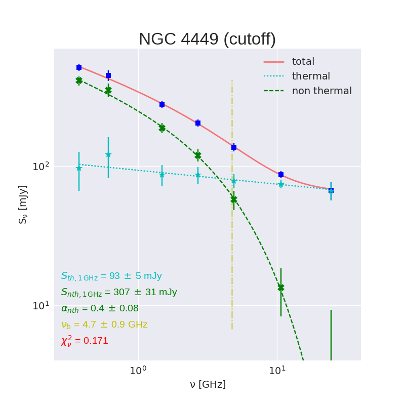
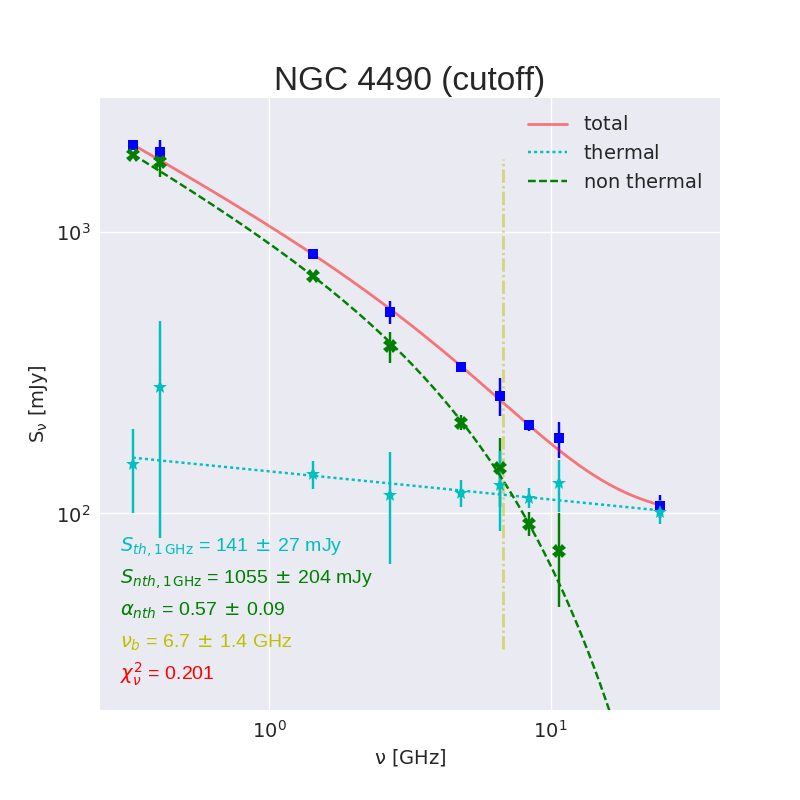
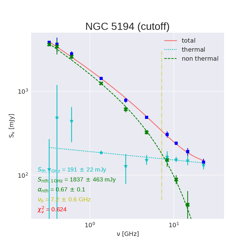
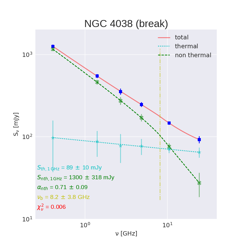
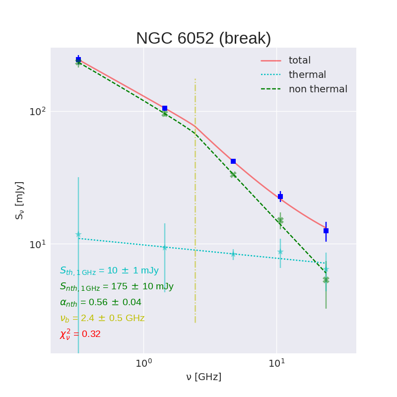
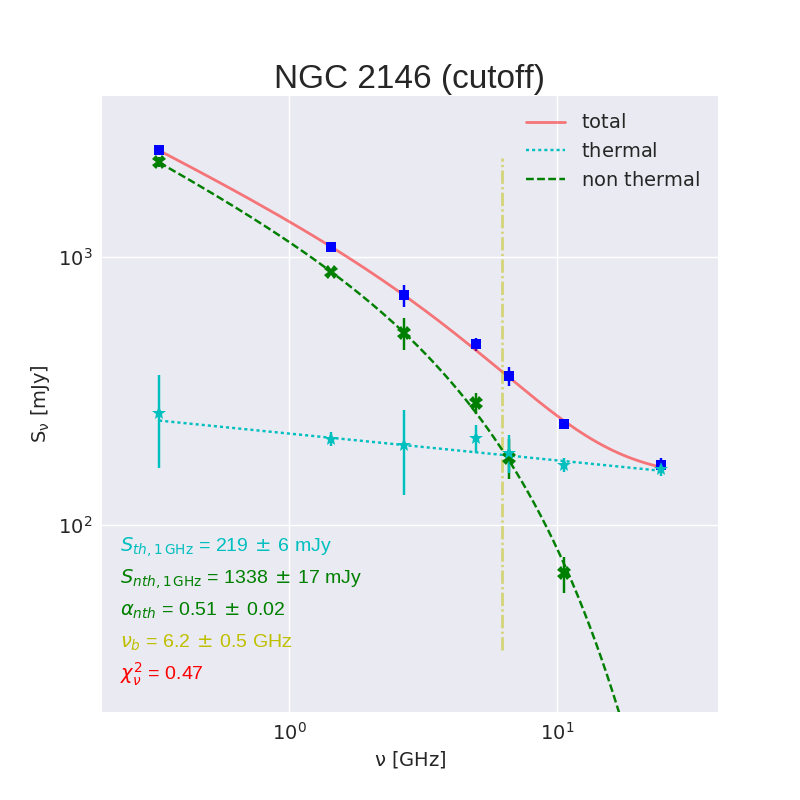
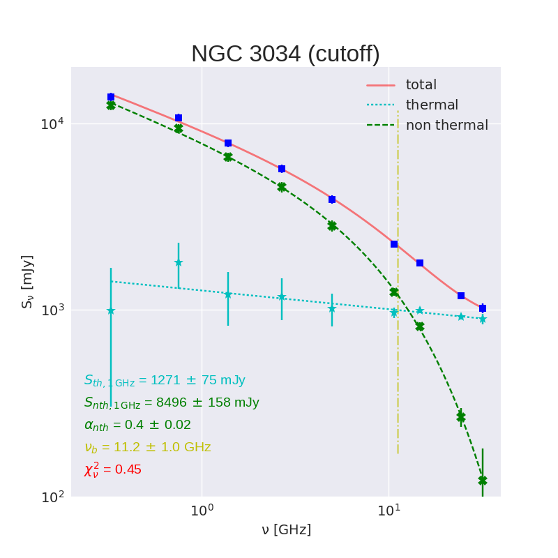
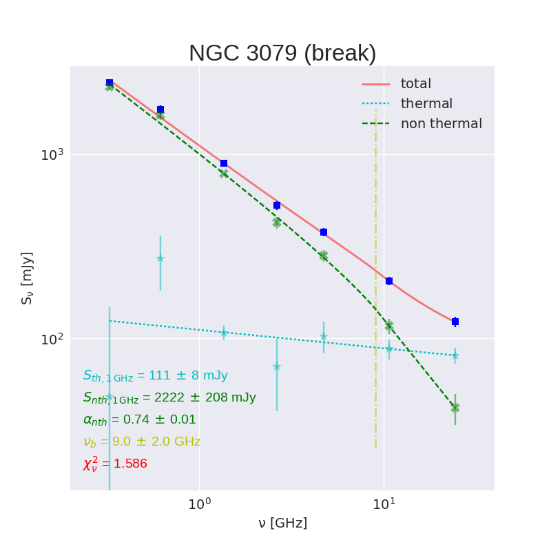
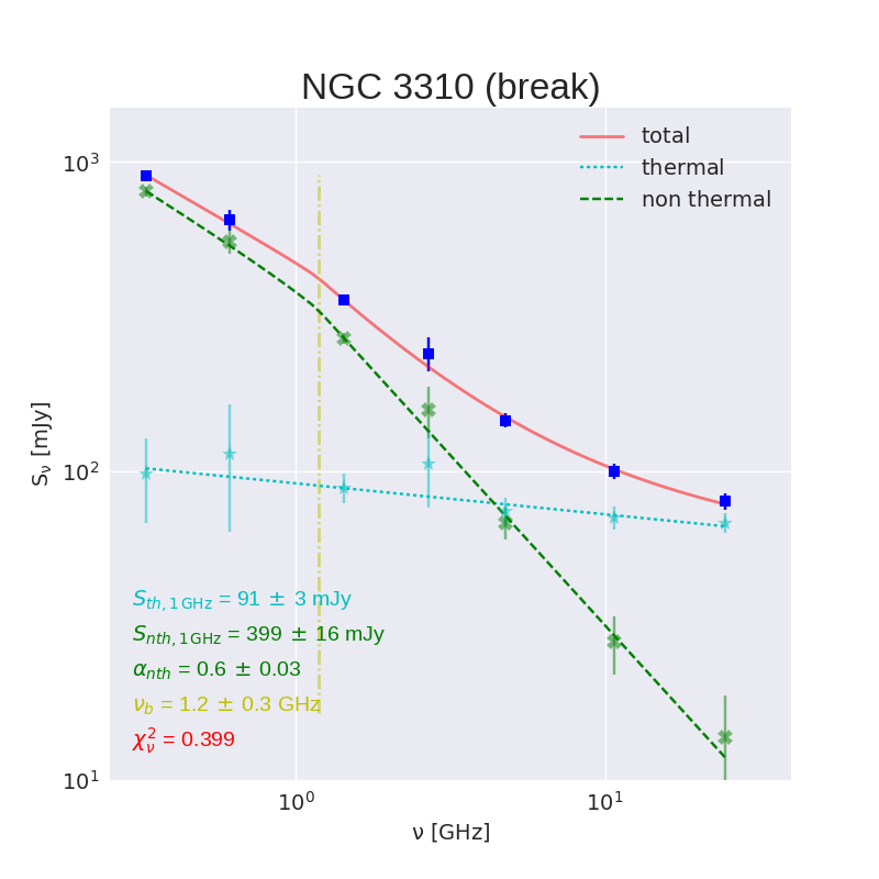
Fig. 1 shows the best fits out of the four tested cases (constant, curved, break, or cutoff, solid red line). In these plots, we also display the free-free (thermal, dotted cyan line) and synchrotron (nonthermal, dashed green line) components of the models. The observed radio continuum flux densities minus the fitted nonthermal component is represented by cyan stars, while the observed minus the fitted thermal component is depicted by green crosses. The optimal values of the parameters are listed in the lower left part of the figure, and their errors are given in terms of the standard deviation of 1000 generated models (for more detailed information see App. B).
In Table 3 we compile the fit results obtained from the best-fit model, with the total flux density at 1 GHz and its error listed in Col. 2, the fraction of thermal emission at 1 GHz and its error in Col. 3, the nonthermal spectral index and its error in Col. 4, the break frequency in GHz and its error in Col. 5, the reduced in Col. 6, and the name of the best-fit model in Col. 7.
| Galaxy | best fit | |||||
|---|---|---|---|---|---|---|
| [mJy] | [GHz] | |||||
| II Zw 40 | - | |||||
| II Zw 70 | constant | |||||
| IC 10 | constant | |||||
| NGC 1569 | cutoff | |||||
| NGC 4449 | cutoff | |||||
| \hdashlineNGC 4490 | cutoff | |||||
| NGC 4631 | cutoff | |||||
| NGC 5194 | cutoff | |||||
| \hdashlineNGC 4038 | break | |||||
| NGC 6052 | break | |||||
| \hdashlineNGC 2146 | cutoff | |||||
| NGC 3034 | cutoff | |||||
| NGC 3079 | break | |||||
| NGC 3310 | break |
In general, the best fit was selected as the lowest reduced chi-squared, . Apart from this, the resulting thermal emission was an asset of whether the fits are physically meaningful. Thus, we rejected fits in spite of an acceptable if the fitted thermal radio emission was unphysically low. In addition, an important test was to look at the resulting thermal flux densities obtained at each frequency after subtracting the computed nonthermal flux density from the total (observed). A fit makes only sense if the resulting thermal flux densities so obtained obey to the expected optically thin spectrum with slope . This is shown by the blue data points in each diagram, with the errors taken from those of the measured total flux densities.
The most striking result of our fits is that most objects need strongly curved (break or cutoff) synchrotron spectra in order to satisfactorily fit the total radio spectrum. Apparent exceptions are the three dwarf galaxies IC 10, II Zw 40, and II Zw 70. IC 10 and II Zw 70 can be well fitted by a constant synchrotron spectrum, while in case of II Zw 40 it is only at the lowest frequencies that nonthermal emission becomes evident. We therefore decided to fit a power-law only to its high-frequency data, obtaining an optically thin thermal spectrum with slope . This spectrum is then extrapolated to the lower frequencies at which we retrieve the nonthermal flux densities by subtracting the extrapolation from the measured fluxes. In Fig. 1 the dashed cyan line shows the fit to the three high-frequency data, yielding a perfect optically thin thermal spectrum. At the two low frequencies we have subtracted the extrapolated thermal flux densities from those observed, such as to yield the nonthermal spectrum.
We have also produced fits to this spectrum in which is limited to 1.0, 0.9, 0.8, 0.7, and 0.6. We note that may take values as low as 0.8, and the total fit is still compatible with the error bars of the observational data. The thermal spectrum is a little lower in this case and, as expected, is worse. Values of 0.7 and 0.6 make the total fit to go below the first data point. We also tried to fit with maximum values of 0.5 and 0.4, but the fits did not converge.
Obviously, the BCDGs and IC 10 are dominated by the thermal radio emission ( at 1 GHz) so that we cannot draw any firm conclusions about the shape of the synchrotron spectra at all.
Also for NGC 3079 a straight or curved synchrotron spectrum formally gives the best fit, and for NGC 4038, all 4 fits are acceptable. However, the thermal flux density obtained for the constant/curved fits are rather low. Compared to the H data they would require internal extinctions of 25 (for NGC 3079) and 10 (for NGC 4038) which seems rather low for these edge-on, highly extinguished galaxies.
For 10 of the 14 galaxies, the best-fit spectrum is that with either a break or a cutoff. For 5 galaxies, the values are very similar in both cases (within a factor of 1.5), and for all 10 galaxies both break and cutoff give acceptable fits. In addition, the broad radio range covered by our data in most of these galaxies renders both, the steepening of the spectrum starting at GHz, due to the strong curvature of the synchrotron emission, and the subsequent flattening due to the dominance of the thermal radio emission (above 10 GHz) visible in the measured spectra! The most noticeable cases are NGC 2146, NGC 4449, NGC 4631, and NGC 5194, but also in NGC 1569, NGC 3034, and NGC 3310 this trend is visible. The fact that we directly observe the steepening and subsequent flattening in the data lends support for the reality of the pronounced curvature of the synchrotron spectra that our fitting procedure yields.

6 Discussion
6.1 Comparision of thermal radio and H emission
We have used the thermal flux densities resulting from our spectral decomposition to compare them with what is predicted from the observed H fluxes corrected for N ii emission and Galactic extinction (Table LABEL:tab:ancillary_data). We used the relation derived by Lequeux (1980), converted from H to H:
| (17) |
The extinction is then calculated via
| (18) |
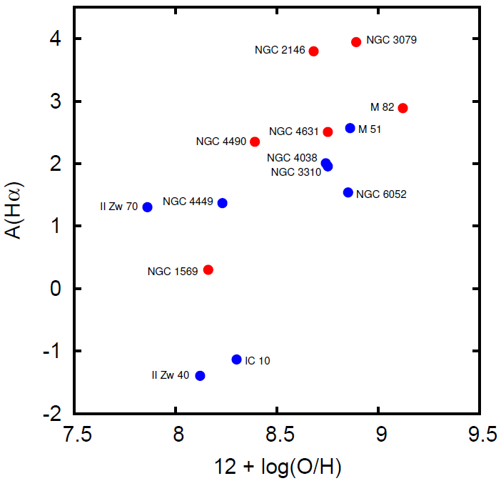
Since extinction is caused by the dust in the galaxy planes, we have plotted in Fig. 2 the extinction resulting from Eqn. 18 vs. the metallicity, for which we have collected the quantity from the literature (Table LABEL:tab:ancillary_data). As is to be expected, there is a trend of increasing extinction with increasing metallicity, with the highly inclined spiral galaxies having the largest extinctions. Dwarf galaxies are known to possess lower metallicities and thus have a low dust content, hence they are found in the lower left part of the diagram. The values for IC 10 and II Zw 40 are even negative, which is most likely due to an overestimate of the Galactic extinction which is very high in both cases (34 for IC 10 and 18 for II Zw 40). An underestimate of the thermal radio emission is unlikely in these two cases because for II Zw 40 the thermal radio emission is directly given by the high-frequency data and for IC 10 the result for the thermal fraction yields very similar values for all fits.
6.2 Thermal fraction
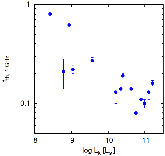
In Fig. 3 we show the fraction of thermal emission at 1 GHz resulting from our spectral fits, plotted vs. the K-band luminosity of the galaxies. Since this luminosity is a measure for the stellar mass, the diagram clearly indicates a decreasing relative amount of nonthermal radiation as we move to small stellar masses. In fact, the left half of this plot contains all the dwarf galaxies in our sample. This result corroborates the early conjecture of Klein et al. (1991) that the lowest-mass galaxies are unable to retain the recently produced cosmic rays. Alternatively, the high thermal fraction in the most extreme galaxies II Zw 40 and II Zw 70 might be the result of a temporal effect. Both galaxies are currently experiencing a strong and very recent starburst, with an age of only Myr, derived from the presence of Wolf-Rayet feature in their spectra. This means that the newly formed, ionizing stars are contributing to the thermal radio emission, but no supernovae may have gone off yet. Hence, the observed synchrotron radiation may have been produced during a previous epoch of star formation. We also compare the thermal fraction with the SFR (from Tab. LABEL:tab:ancillary_data but found no correlation.
It is important to note here that for some of the galaxies in our sample the amount of thermal emission resulting from our analysis is higher than thought hitherto, which has consequences for any conjectures based upon the thermal radio continuum in star-forming galaxies. This is particularly true for higher frequencies where the cutoff/break lowers the synchrotron emission considerably. At 10 GHz, the mean thermal fraction for the galaxies is 0.6 – considerably more than what was believed so far.
6.3 Injection spectra
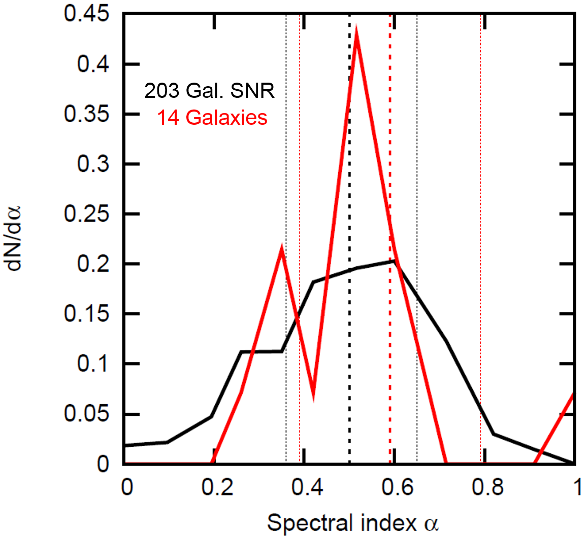
In Fig. 4 a superposition of the low-frequency spectral indices of the synchrotron radiation of our galaxy sample with the spectral indices of Galactic supernova remnants (SNR) is shown, the latter data taken from the catalogue of Green (2014). The two distributions are rather similar, albeit the statistics are vastly different (203 vs. 14 objects). The resulting values of the mean and standard deviation are , and , for the SNR and galaxies, respectively. Both, the mean and the rms are rather similar, possibly suggesting that the synchrotron spectra that we measure at low radio frequencies reflect the injection spectra of the SNR.
An outlier is II Zw 70, which has a low-frequency spectral index of . Such a steep spectrum is indicative of the impact of synchrotron and inverse-Compton losses which have steepened the injection spectral index by . It is unclear why II Zw 70 is so different from the rest of the galaxies. The SFR per , which can be taken as a measure of the capability of the galaxy to expell material into the halo, is similar to that of the other starburst galaxies, such as M 82 or NGC 1569 (but more than a factor of 10 lower than for the otherwise similar BCDG II Zw 40).
| Galaxy | Radio Size | 111111The magnetic field is calculated with the minimum energy assumption. | Shape | |
| [kpc] | [G] | [GeV] | ||
| II Zw 40 | 0.8 | 29 | - | - |
| II Zw 70 | 0.6 | 40 | - | constant |
| IC 10 | 1.3 | 14 | - | constant |
| NGC 1569 | 2.5 | 16 | 6.8 | cutoff |
| NGC 4449 | 5.0 | 14 | 4.6 | cutoff |
| \hdashlineNGC 4490 | 10 | 20 | 4.6 | cutoff |
| NGC 4631 | 22 | 13 | 5.6 | cutoff |
| NGC 5194 | 15 | 18 | 5.0 | cutoff |
| \hdashlineNGC 4038 | 18 | 27 | - | break |
| NGC 6052 | 4.0 | 71 | - | break |
| \hdashlineNGC 2146 | 10 | 40 | 3.1 | cutoff |
| NGC 3034 | 1.7 | 66 | 3.3 | cutoff |
| NGC 3079 | 13 | 32 | - | break |
| NGC 3310 | 4.4 | 39 | - | break |
6.4 Spectral breaks and cutoffs
For the majority of our galaxies, the fitting of their radio spectra shows the need of a break of the synchrotron spectra in the range of GHz, corresponding to particle energies of GeV, depending on the magnetic-field strengths (see Table 4). The low-frequency spectrum in all cases except II Zw 70 has a spectral index in the range of what is found for SNRs, suggesting that the relativistic electrons emitting in this range have not suffered any significant synchrotron and inverse-Compton losses that would steepen their spectrum. The steep high-frequency spectrum indicates that synchrotron or inverse-Compton losses are important (in the case of a break) or a complete lack of relativistic electrons above GeV (in the case of a cutoff).
As outlined in Sect. 4.1, a sharp break can be explained in an open box-model with convection. The break is produced because high-energy electrons, emitting at frequencies above the break, suffer substantial synchrotron or inverse-Compton losses before they arrive at the edge of the halos, whereas low-energy electrons do not. We can estimate the half-lifetime of the relativistic electrons emitting the synchrotron radiation at the break freqeuncy, which is determined by synchrotron and inverse-Compton losses (see, e.g., Klein & Fletcher 2015):
| (19) |
Here, is the energy of the relativistic particles, is the total magnetic-field strength, and is the field strength equivalent to the energy density of the local radiation field. The latter can be obtained via
| (20) |
Here, is the bolometric luminosity of a region of size . Kennicutt et al. (2007) have measured the quantity at 24 m (which approximates the luminosity) for a number of H ii regions in M 51, with typical values of erg s-1, obtained with aperture sizes of 13′′ (hence, pc). Plugging this into Eqn. (20), we obtain G. The strength of the magnetic field in our sample galaxies is between G and G (Table 4). This implies a range for the particle half-lifetimes of between yr and yr (Tev and PeV particles enter the GeV regime on time scales much shorter than any dynamical time scales under conditions considered above). Assuming a vertical halo size of about 250 pc, this implies convection speeds of between 10 and 300 km s-1, which is reasonable. In order to test this interpretation, it would be useful to carry out a similar analysis for quiescent galaxies with a low star-formation rate per area for which we would expect much lower vertical propagation of the relativistic electrons.
A cutoff in the relativistic electron distribution is more difficult to explain. Energy losses can produce a cutoff only in a single-injection scenario where radiative ageing depopulates the high-energy part of the relativistic electron distribution with time. This situation is unrealistic for the integrated radio emission of an entire galaxy. The acceleration process of cosmic rays in SNRs is effective up to TeV energies and the synchrotron spectra of young SNRs can be observed up to X-ray energies. At high energies, the short synchrotron energy loss time in the strong magnetic fields (G) in SNR (Völk et al. 2005) is expected to produce a steepening of the electron injection spectrum. This can be seen from Eqn. 19, which for a particle energy of, say, 100 GeV, in a 100 G magnetic field yields a lifetime of yr. This is comparable to the Sedov phase of a SNR ( yr) so that at energies above GeV synchrotron cooling should be relevant and produce a steeper injection spectrum above Hz. However, the breaks/cutoffs that we infer are at much lower particle energies and do therefore not probe this process. Thus, in the framework of the simple models considered here, it is unclear which process could produce a cutoff in the synchrotron spectrum. It is, however, obvious that this must have to do with the relative time scales of energy gain, losses and escape of the relativistic electrons, as discussed by Schlickeiser (1984).
7 Summary and conclusions
We have analyzed the radio continuum spectra of 14 star-forming galaxies by fitting nonthermal (synchrotron) and thermal (free-free) radiation laws to carefully selected measurements, covering a frequency range of 300 MHz to 24.5 GHz (32 GHz in case of M 82). The 24.5-GHz measurements, mostly unpublished to date, are crucial for a more reliable separation of the thermal and nonthermal components in this analysis.
We find that the majority of the synchrotron spectra are not simple power-laws as believed hitherto. The curved shape of the synchrotron spectrum is clearly visible in many of the total radio spectra, which steepen over a range of several GHz and flatten at higher frequencies due to the thermal radio emission. Our fitting shows that the lowest values of the reduced result for synchrotron spectra with a mean slope in the low-frequency regime, and a break or an exponential decline in the frequency range of GHz. There are only one galaxy that shows pure power-laws (the dwarf galaxy IC 10). In the case of the BCDGs II Zw 40 and II Zw 70 only the slope (and not the shape) of the synchrotron spectrum can be worked out, since a deviation from a purely thermal spectrum is only evident at the lowest frequencies involved.
For the bulk of the sample galaxies, simple power-laws or mildly curved synchrotron spectra lead to unrealistic low thermal flux densities (frequently ), and/or to strong deviations from the expected optically thin free-free spectra with slope in the fits. Assuming energy equipartition between relativistic particles and magnetic fields, the cutoff and break frequencies translate into energies in the range of GeV. The average spectral index of the low-frequency spectra obtained here is comparable to that found for Galactic (shell-type) supernova remnants.
A comparison of the thermal flux densities resulting from our fits with the (foreground-corrected) H fluxes yields the extinction, which increases with metallicity. The fraction of thermal emission at 1 GHz is higher in some of our galaxies than believed hitherto, and the discrepancy increases towards higher frequencies where the mean thermal fraction is . It is highest in the dwarf galaxies of our sample, which we interpret either in terms of a lack of containment of synchrotron emission in these low-mass systems, or alternatively, in the case of II Zw 40 and II Zw 70, as a time effect due to a very young starburst.
The asymptotic low-frequency synchrotron spectra derived here provide a firm ‘leverage’ for low-frequency studies, e.g. with LOFAR. In order to significantly incraese the number of radio continuum spectra of galaxies allowing analyses as presented here, expensive mapping with large single-dish telescopes (Effelsberg, GBT, Sardinia Radio Telescope) in the frequency range of 25 – 40 GHz (so-called Ka-band in radio astronomy) are indispensible.
An interpretation of the rapid declines in the synchrotron spectra (break or exponential cutoff) at GeV particle energies is not obvious, since the relativistic particles gain energies up to the TeV range within the supernovae. In a simple model, a convective wind carrying away the low-energy relativistic electrons could explain a sharp break. The break energy must depend on the relative time scales of energy gain (acceleration), losses (synchrotron and inverse-Compton) and escape of the relativistic electrons.
Acknowledgements.
We wish to thank H. Lesch and R. Schlickeiser for helpful discussions. UK acknowledges financial support by the German Deutsche Forschungsgemeinschaft, DFG project FOR 1254, and is very grateful for the kind hospitality at the Departamento de Física Teórica y del Cosmos, Universidad de Granada. UL and SV acknowledge support by the research projects AYA2014-53506-P from the Spanish Ministerio de Economía y Competitividad, from the European Regional Development Funds (FEDER) and the Junta de Andalucía (Spain) grants FQM108. This research has made use of the NASA/IPAC Extragalactic Database (NED), which is operated by the Jet Propulsion Laboratory, California Institute of Technology, under contract with the National Aeronautics and Space Administration. We also acknowledge the use of the HyperLeda database (http://leda.univ-lyon1.fr). This research made use of astropy, a community-developed core python (http://www.python.org) package for Astronomy (Astropy Collaboration et al. 2013); ipython (Pérez & Granger 2007); matplotlib (Hunter 2007); numpy (van der Walt et al. 2011); scipy (Jones et al. 2001–). Finally, we are very greatful to the referee for her/his comments, which helped to improve the manuscript.References
- Adebahr et al. (2013) Adebahr, B., Krause, M., Klein, U., et al. 2013, A&A, 555, A23
- Astropy Collaboration et al. (2013) Astropy Collaboration, Robitaille, T. P., Tollerud, E. J., et al. 2013, A&A, 558, A33
- Baars et al. (1977) Baars, J. W. M., Genzel, R., Pauliny-Toth, I. I. K., & Witzel, A. 1977, A&A, 61, 99
- Balkowski et al. (1978) Balkowski, C., Chamaraux, P., & Weliachew, L. 1978, A&A, 69, 263
- Bastian et al. (2009) Bastian, N., Trancho, G., Konstantopoulos, I. S., & Miller, B. W. 2009, ApJ, 701, 607
- Basu et al. (2017) Basu, A., Mao, S. A., Kepley, A. A., et al. 2017, MNRAS, 464, 1003
- Beck et al. (1987) Beck, R., Klein, U., & Wielebinski, R. 1987, A&A, 186, 95
- Becker et al. (1991) Becker, R. H., White, R. L., & Edwards, A. L. 1991, ApJS, 75, 1
- Berezhko & Völk (1997) Berezhko, E. G. & Völk, H. J. 1997, Astroparticle Physics, 7, 183
- Branch et al. (1999) Branch, M. A., Coleman, T. F., & Li, Y. 1999, SIAM J. Sci. Comput., 21, 1
- Braun et al. (2007) Braun, R., Oosterloo, T. A., Morganti, R., Klein, U., & Beck, R. 2007, A&A, 461, 455
- Brown et al. (2014) Brown, M. J. I., Moustakas, J., Smith, J.-D. T., et al. 2014, ApJS, 212, 18
- Chyży & Beck (2004a) Chyży, K. T. & Beck, R. 2004a, A&A, 417, 541
- Chyży & Beck (2004b) Chyży, K. T. & Beck, R. 2004b, A&A, 417, 541
- Chyży et al. (2000) Chyży, K. T., Beck, R., Kohle, S., Klein, U., & Urbanik, M. 2000, A&A, 355, 128
- Chyży et al. (2016) Chyży, K. T., Drzazga, R. T., Beck, R., et al. 2016, ApJ, 819, 39
- Chyży et al. (2003) Chyży, K. T., Knapik, J., Bomans, D. J., et al. 2003, A&A, 405, 513
- Chyży et al. (2011) Chyży, K. T., Weżgowiec, M., Beck, R., & Bomans, D. J. 2011, A&A, 529, A94
- Clemens et al. (1999) Clemens, M. S., Alexander, P., & Green, D. A. 1999, MNRAS, 307, 481
- Condon (1987) Condon, J. J. 1987, ApJS, 65, 485
- Condon et al. (1998) Condon, J. J., Cotton, W. D., Greisen, E. W., et al. 1998, AJ, 115, 1693
- Dale et al. (2009) Dale, D. A., Cohen, S. A., Johnson, L. C., et al. 2009, ApJ, 703, 517
- de Bruyn (1977) de Bruyn, A. G. 1977, A&A, 58, 221
- de Jong (1967) de Jong, M. L. 1967, ApJ, 150, 1
- Deeg et al. (1993) Deeg, H.-J., Brinks, E., Duric, N., Klein, U., & Skillman, E. 1993, ApJ, 410, 626
- Drury et al. (1994) Drury, L. O., Aharonian, F. A., & Voelk, H. J. 1994, A&A, 287, 959
- Dumke et al. (1995) Dumke, M., Krause, M., Wielebinski, R., & Klein, U. 1995, A&A, 302, 691
- Duric et al. (1988) Duric, N., Bourneuf, E., & Gregory, P. C. 1988, AJ, 96, 81
- Duric & Seaquist (1988) Duric, N. & Seaquist, E. R. 1988, ApJ, 326, 574
- Duric et al. (1983) Duric, N., Seaquist, E. R., Crane, P. C., Bignell, R. C., & Davis, L. E. 1983, ApJ, 273, L11
- Duric et al. (1986) Duric, N., Seaquist, E. R., Crane, P. C., & Davis, L. E. 1986, ApJ, 304, 82
- Ekers & Sancisi (1977) Ekers, R. D. & Sancisi, R. 1977, A&A, 54, 973
- Emerson et al. (1979) Emerson, D. T., Klein, U., & Haslam, C. G. T. 1979, A&A, 76, 92
- Engelbracht et al. (2008) Engelbracht, C. W., Rieke, G. H., Gordon, K. D., et al. 2008, ApJ, 678, 804
- Fletcher et al. (2011) Fletcher, A., Beck, R., Shukurov, A., Berkhuijsen, E. M., & Horellou, C. 2011, MNRAS, 412, 2396
- Gil de Paz et al. (2003) Gil de Paz, A., Madore, B. F., & Pevunova, O. 2003, ApJS, 147, 29
- Gioia & Gregorini (1980) Gioia, I. M. & Gregorini, L. 1980, A&AS, 41, 329
- Gioia et al. (1982) Gioia, I. M., Gregorini, L., & Klein, U. 1982, A&A, 116, 164
- Golla (1999) Golla, G. 1999, A&A, 345, 778
- Green (2014) Green, D. A. 2014, ArXiv e-prints
- Gregory & Condon (1991) Gregory, P. C. & Condon, J. J. 1991, ApJS, 75, 1011
- Griffith et al. (1994) Griffith, M. R., Wright, A. E., Burke, B. F., & Ekers, R. D. 1994, ApJS, 90, 179
- Haynes et al. (1975) Haynes, R. F., Huchtmeier, W. K. G., & Siegman, B. C. 1975, A compendium of radio measurements of bright galaxies
- Heidmann (1979) Heidmann, J. 1979, in Extragalactic Astronomy - Meeting “Sol-Espace”, ed. C. Balkowski-Mauger, 205
- Heidmann et al. (1982) Heidmann, J., Klein, U., & Wielebinski, R. 1982, A&A, 105, 188
- Holtzman et al. (1996) Holtzman, J. A., Watson, A. M., Mould, J. R., et al. 1996, AJ, 112, 416
- Hummel (1980) Hummel, E. 1980, A&AS, 41, 151
- Hummel (1991) Hummel, E. 1991, A&A, 251, 442
- Hummel et al. (1991) Hummel, E., Beck, R., & Dahlem, M. 1991, A&A, 248, 23
- Hummel & Dettmar (1990a) Hummel, E. & Dettmar, R.-J. 1990a, A&A, 236, 33
- Hummel & Dettmar (1990b) Hummel, E. & Dettmar, R.-J. 1990b, A&A, 236, 33
- Hummel et al. (1985) Hummel, E., Pedlar, A., Davies, R. D., & van der Hulst, J. M. 1985, A&AS, 60, 293
- Hunter (2007) Hunter, J. D. 2007, Computing In Science & Engineering, 9, 90
- Irwin et al. (2012) Irwin, J., Beck, R., Benjamin, R. A., et al. 2012, AJ, 144, 44
- Irwin & Saikia (2003) Irwin, J. A. & Saikia, D. J. 2003, MNRAS, 346, 977
- Israel & de Bruyn (1988) Israel, F. P. & de Bruyn, A. G. 1988, A&A, 198, 109
- Israel & Mahoney (1990) Israel, F. P. & Mahoney, M. J. 1990, ApJ, 352, 30
- Israel & van der Hulst (1983) Israel, F. P. & van der Hulst, J. M. 1983, AJ, 88, 1736
- Jaffe & Perola (1973) Jaffe, W. J. & Perola, G. C. 1973, A&A, 26, 423
- Jaffe et al. (1978) Jaffe, W. J., Perola, G. C., & Tarenghi, M. 1978, ApJ, 224, 808
- Jarrett et al. (2000) Jarrett, T. H., Chester, T., Cutri, R., et al. 2000, AJ, 119, 2498
- Jarrett et al. (2003) Jarrett, T. H., Chester, T., Cutri, R., Schneider, S. E., & Huchra, J. P. 2003, AJ, 125, 525
- Jones et al. (2001–) Jones, E., Oliphant, T., Peterson, P., et al. 2001–, SciPy: Open source scientific tools for Python, [Online; accessed ¡today¿]
- Kardashev (1962) Kardashev, N. S. 1962, Sov. Ast., 6, 317
- Kazès et al. (1970) Kazès, I., Le Squeren, A. M., & Nguyen-Quang-Rieu. 1970, Astrophys. Lett., 6, 193
- Kehrig et al. (2008) Kehrig, C., Vílchez, J. M., Sánchez, S. F., et al. 2008, A&A, 477, 813
- Kellermann et al. (1969) Kellermann, K. I., Pauliny-Toth, I. I. K., & Williams, P. J. S. 1969, ApJ, 157, 1
- Kennicutt et al. (2007) Kennicutt, Jr., R. C., Calzetti, D., Walter, F., et al. 2007, ApJ, 671, 333
- Kennicutt et al. (2009) Kennicutt, Jr., R. C., Hao, C.-N., Calzetti, D., et al. 2009, ApJ, 703, 1672
- Kennicutt et al. (2008) Kennicutt, Jr., R. C., Lee, J. C., Funes, José G., S. J., Sakai, S., & Akiyama, S. 2008, ApJS, 178, 247
- Kepley et al. (2010) Kepley, A. A., Mühle, S., Everett, J., et al. 2010, ApJ, 712, 536
- Klein (1983) Klein, U. 1983, A&A, 121, 150
- Klein (1988) Klein, U. 1988, PhD thesis, Habilitation Thesis, Univ. Bonn, (1988)
- Klein & Emerson (1981) Klein, U. & Emerson, D. T. 1981, A&A, 94, 29
- Klein & Fletcher (2015) Klein, U. & Fletcher, A. 2015, Galactic and Intergalactic Magnetic Fields
- Klein & Gräve (1986) Klein, U. & Gräve, R. 1986, A&A, 161, 155
- Klein et al. (1983) Klein, U., Gräve, R., & Wielebinski, R. 1983, A&A, 117, 332
- Klein et al. (1996) Klein, U., Hummel, E., Bomans, D. J., & Hopp, U. 1996, A&A, 313, 396
- Klein et al. (1991) Klein, U., Weiland, H., & Brinks, E. 1991, A&A, 246, 323
- Klein et al. (1984a) Klein, U., Wielebinski, R., & Beck, R. 1984a, A&A, 135, 213
- Klein et al. (1988) Klein, U., Wielebinski, R., & Morsi, H. W. 1988, A&A, 190, 41
- Klein et al. (1984b) Klein, U., Wielebinski, R., & Thuan, T. X. 1984b, A&A, 141, 241
- Kobulnicky & Skillman (1997) Kobulnicky, H. A. & Skillman, E. D. 1997, ApJ, 489, 636
- Kregel & Sancisi (2001) Kregel, M. & Sancisi, R. 2001, A&A, 376, 59
- Lequeux (1971) Lequeux, J. 1971, A&A, 15, 30
- Lequeux (1980) Lequeux, J. 1980, in Saas-Fee Advanced Course 10: Star Formation, ed. A. Maeder & L. Martinet, 9999
- Lisenfeld et al. (1996) Lisenfeld, U., Alexander, P., Pooley, G. G., & Wilding, T. 1996, MNRAS, 281, 301
- Lisenfeld et al. (2004) Lisenfeld, U., Wilding, T. W., Pooley, G. G., & Alexander, P. 2004, MNRAS, 349, 1335
- Maehara et al. (1985) Maehara, H., Inoue, M., Takase, B., & Noguchi, T. 1985, PASJ, 37, 451
- Magrini & Gonçalves (2009) Magrini, L. & Gonçalves, D. R. 2009, MNRAS, 398, 280
- Mao et al. (2015) Mao, S. A., Zweibel, E., Fletcher, A., Ott, J., & Tabatabaei, F. 2015, ApJ, 800, 92
- Marvil et al. (2015) Marvil, J., Owen, F., & Eilek, J. 2015, AJ, 149, 32
- McCutcheon (1973) McCutcheon, W. H. 1973, AJ, 78, 18
- Mora & Krause (2013) Mora, S. C. & Krause, M. 2013, A&A, 560, A42
- Moustakas & Kennicutt (2006) Moustakas, J. & Kennicutt, Jr., R. C. 2006, ApJS, 164, 81
- Moustakas et al. (2010) Moustakas, J., Kennicutt, Jr., R. C., Tremonti, C. A., et al. 2010, ApJS, 190, 233
- Mulcahy et al. (2014) Mulcahy, D. D., Horneffer, A., Beck, R., et al. 2014, A&A, 568, A74
- Neininger (1992) Neininger, N. 1992, A&A, 263, 30
- Nikiel-Wroczyński et al. (2016) Nikiel-Wroczyński, B., Jamrozy, M., Soida, M., Urbanik, M., & Knapik, J. 2016, MNRAS, 459, 683
- Niklas et al. (1995) Niklas, S., Klein, U., Braine, J., & Wielebinski, R. 1995, A&AS, 114, 21
- Niklas et al. (1997) Niklas, S., Klein, U., & Wielebinski, R. 1997, A&A, 322, 19
- Pérez & Granger (2007) Pérez, F. & Granger, B. E. 2007, Computing in Science and Engineering, 9, 21
- Perley & Butler (2013) Perley, R. A. & Butler, B. J. 2013, ApJS, 204, 19
- Pfleiderer et al. (1980) Pfleiderer, J., Durst, C., & Gebler, K.-H. 1980, MNRAS, 192, 635
- Pilyugin & Thuan (2007) Pilyugin, L. S. & Thuan, T. X. 2007, ApJ, 669, 299
- Purkayastha (2014) Purkayastha, A. 2014, PhD thesis, Thesis (Ph.D.) – University Bonn, 2014
- Rengelink et al. (1997) Rengelink, R. B., Tang, Y., de Bruyn, A. G., et al. 1997, A&AS, 124, 259
- Robertson et al. (2013) Robertson, P., Shields, G. A., Davé, R., Blanc, G. A., & Wright, A. 2013, ApJ, 773, 4
- Sage et al. (1993) Sage, L. J., Loose, H. H., & Salzer, J. J. 1993, A&A, 273, 6
- Schlickeiser (1984) Schlickeiser, R. 1984, A&A, 136, 227
- Segalovitz (1977) Segalovitz, A. 1977, A&A, 54, 703
- Skillman & Klein (1988) Skillman, E. D. & Klein, U. 1988, A&A, 199, 61
- Slee (1995) Slee, O. B. 1995, Australian Journal of Physics, 48, 143
- Sramek (1975) Sramek, R. 1975, AJ, 80, 771
- Srivastava et al. (2014) Srivastava, S., Kantharia, N. G., Basu, A., Srivastava, D. C., & Ananthakrishnan, S. 2014, MNRAS, 443, 860
- Sulentic (1976) Sulentic, J. W. 1976, ApJS, 32, 171
- Tabatabaei et al. (2017) Tabatabaei, F. S., Schinnerer, E., Krause, M., et al. 2017, ApJ, 836, 185
- Thuan & Izotov (2005) Thuan, T. X. & Izotov, Y. I. 2005, ApJS, 161, 240
- Tovmassian (1968) Tovmassian, H. M. 1968, Australian Journal of Physics, 21, 193
- van der Hulst (1979) van der Hulst, J. M. 1979, A&A, 71, 131
- van der Kruit & de Bruyn (1976) van der Kruit, P. C. & de Bruyn, A. G. 1976, A&A, 48, 373
- van der Walt et al. (2011) van der Walt, S., Colbert, S. C., & Varoquaux, G. 2011, Computing in Science Engineering, 13, 22
- Varenius et al. (2015) Varenius, E., Conway, J. E., Martí-Vidal, I., et al. 2015, A&A, 574, A114
- Viallefond et al. (1980) Viallefond, F., Allen, R. J., & de Boer, J. A. 1980, A&A, 82, 207
- Völk et al. (2005) Völk, H. J., Berezhko, E. G., & Ksenofontov, L. T. 2005, A&A, 433, 229
- Werner (1988) Werner, W. 1988, A&A, 201, 1
- Wielebinski & von Kap-Herr (1977) Wielebinski, R. & von Kap-Herr, A. 1977, A&A, 59, L17
- Williams & Bower (2010) Williams, P. K. G. & Bower, G. C. 2010, ApJ, 710, 1462
- Wynn-Williams & Becklin (1986) Wynn-Williams, C. G. & Becklin, E. E. 1986, ApJ, 308, 620
Appendix A Flux densities
| Frequency | Flux density | Error | Reference |
|---|---|---|---|
| 0.325 | 38 | 4 | Deeg et al. (1993) |
| 1.459 | 30.1 | 0.4 | Klein et al. (1991), Deeg et al. (1993) |
| 4.88 | 21.5 | 1.9 | Jaffe et al. (1978), Klein et al. (1984b), Klein et al. (1991) |
| 10.63 | 20.1 | 1.5 | Skillman & Klein (1988), Klein et al. (1984b) |
| 24.500 | 18 | 4 | Klein et al. (1984b) |
| Frequency | Flux density | Error | Reference |
|---|---|---|---|
| 0.327 | 11.2 | 2.0 | Skillman & Klein (1988) |
| 0.609 | 6.5 | 0.8 | Skillman & Klein (1988) |
| 1.440 | 4.56 | 0.34 | Wynn-Williams & Becklin (1986), Balkowski et al. (1978) |
| 4.795 | 3.04 | 0.13 | Klein et al. (1984b), Wynn-Williams & Becklin (1986), Skillman & Klein (1988) |
| 10.700 | 2.73 | 0.20 | Skillman & Klein (1988), Klein et al. (1984b) |
| Frequency | Flux density | Error | Reference |
|---|---|---|---|
| 0.327 | 352 | 20 | WENSS, this work |
| 1.43 | 377 | 6 | this work |
| 2.64 | 283 | 20 | Chyży et al. (2011) (recomputed) |
| 4.82 | 219 | 8 | Klein et al. (1983), Klein & Gräve (1986), Becker et al. (1991) |
| 10.575 | 162 | 8 | Klein & Gräve (1986), Chyży et al. (2003) |
| 24.5 | 118 | 18 | Klein & Gräve (1986) |
| Frequency | Flux density | Error | Reference |
|---|---|---|---|
| 0.350 | 750 | 20 | Purkayastha (2014); Ph.D. thesis, Univ. Bonn |
| 0.610 | 610 | 20 | Israel & de Bruyn (1988) |
| 1.415 | 425 | 20 | Hummel (1980), Israel & de Bruyn (1988) |
| 2.700 | 318 | 20 | Pfleiderer et al. (1980), Sulentic (1976) |
| 4.800 | 233 | 20 | Klein & Gräve (1986), Gregory & Condon (1991) |
| 8.350 | 176 | 5 | this work |
| 10.700 | 155 | 10 | Klein & Gräve (1986) |
| 15.36 | 116 | 13 | Lisenfeld et al. (2004) |
| 24.500 | 96 | 8 | Klein & Gräve (1986) |
| Frequency | Flux density | Error | Reference |
|---|---|---|---|
| 0.327 | 2520 | 100 | WENSS, this work |
| 1.43 | 1094 | 13 | NVSS, Braun et al. (2007) |
| 2.695 | 720 | 70 | Haynes et al. (1975) |
| 5.000 | 472 | 25 | de Bruyn (1977) |
| 6.630 | 360 | 30 | McCutcheon (1973) |
| 10.625 | 239 | 10 | Niklas et al. (1995), Israel & van der Hulst (1983) |
| 24.500 | 167 | 10 | this work |
| Frequency | Flux density | Error | Reference |
|---|---|---|---|
| 0.327 | 13830 | 690 | Adebahr et al. (2013) |
| 0.750 | 10700 | 500 | Kellermann et al. (1969) |
| 1.388 | 7805 | 385 | Hummel (1980), Adebahr et al. (2013) |
| 2.695 | 5700 | 300 | Kellermann et al. (1969) |
| 5.000 | 3900 | 200 | Kellermann et al. (1969) |
| 10.700 | 2250 | 60 | Klein et al. (1988) |
| 14.700 | 1790 | 40 | Klein et al. (1988) |
| 24.500 | 1190 | 30 | Klein et al. (1988) |
| 32.000 | 1020 | 60 | Klein et al. (1988) |
| Frequency | Flux density | Error | Reference |
|---|---|---|---|
| 0.327 | 2440 | 100 | WENSS, this work |
| 0.615 | 1740 | 90 | Irwin & Saikia (2003) |
| 1.365 | 800 | 10 | Braun et al. (2007) |
| 2.640 | 526 | 30 | this work |
| 4.750 | 377 | 20 | Gioia et al. (1982) |
| 10.650 | 205 | 11 | Gioia et al. (1982) |
| 24.500 | 123 | 8 | this work |
| Frequency | Flux density | Error | Reference |
|---|---|---|---|
| 0.327 | 904 | 30 | WENSS, this work |
| 0.610 | 650 | 50 | van der Kruit & de Bruyn (1976) |
| 1.433 | 357 | 10 | Condon (1987), Hummel et al. (1985) |
| 2.695 | 240 | 30 | van der Kruit & de Bruyn (1976) |
| 4.750 | 146 | 8 | Gioia et al. (1982) |
| 10.650 | 100 | 6 | Gioia et al. (1982), Israel & de Bruyn (1988), Niklas et al. (1995) |
| 24.500 | 80 | 5 | this work |
| Frequency | Flux density | Error | Reference |
|---|---|---|---|
| 0.408 | 1250 | 60 | Slee (1995) |
| 1.410 | 544 | 30 | van der Hulst (1979), Hummel (1980), this work |
| 2.700 | 353 | 30 | de Jong (1967), Tovmassian (1968), Kazès et al. (1970) |
| 4.850 | 246 | 17 | Griffith et al. (1994) |
| 10.550 | 146 | 7 | Niklas et al. (1995), Chyży & Beck (2004b) re-computed |
| 24.500 | 92 | 9 | this work |
| Frequency | Flux density | Error | Reference |
|---|---|---|---|
| 0.376 | 514 | 30 | Purkayastha (2014) |
| 0.609 | 450 | 40 | Klein et al. (1996) |
| 1.427 | 278 | 15 | Condon (1987), NVSS, this work Klein & Emerson (1981) |
| 2.695 | 204 | 12 | this work |
| 4.875 | 137 | 9 | Klein & Gräve (1986), Sramek (1975) |
| 10.650 | 87 | 5 | Israel & van der Hulst (1983), Klein & Gräve (1986), Klein et al. (1996) |
| 24.500 | 67 | 10 | Klein & Gräve (1986) |
| Frequency | Flux density | Error | Reference |
|---|---|---|---|
| 0.327 | 2040 | 50 | WENSS, this work |
| 0.408 | 2099 | 50 | Gioia & Gregorini (1980) |
| 1.430 | 835 | 16 | Lequeux (1971), Viallefond et al. (1980), Condon (1987) |
| 2.695 | 520 | 50 | Kazès et al. (1970) |
| 4.81 | 331 | 13 | Gioia et al. (1982), Nikiel-Wroczyński et al. (2016) |
| 6.630 | 262 | 40 | McCutcheon (1973) |
| 10.700 | 185 | 27 | Klein & Emerson (1981) |
| 24.500 | 106 | 10 | Klein (1983) |
| Frequency | Flux density | Error | Reference |
|---|---|---|---|
| 0.327 | 2993 | 110 | Hummel & Dettmar (1990b), WENSS, this work |
| 0.419 | 2900 | 71 | Gioia & Gregorini (1980), Israel & van der Hulst (1983) |
| 0.610 | 2200 | 100 | Ekers & Sancisi (1977), Werner (1988) |
| 0.835 | 2000 | 100 | Israel & de Bruyn (1988) |
| 1.423 | 1282 | 20 | Ekers & Sancisi (1977), Hummel & Dettmar (1990b), Braun et al. (2007) |
| 2.688 | 835 | 32 | Wielebinski & von Kap-Herr (1977), Werner (1988) |
| 4.750 | 544 | 20 | Wielebinski & von Kap-Herr (1977), Israel & van der Hulst (1983), Werner (1988) |
| 8.35 | 310 | 16 | Mora & Krause (2013) |
| 10.625 | 260 | 10 | Israel & van der Hulst (1983), Dumke et al. (1995) |
| 24.500 | 172 | 15 | this work |
| Frequency | Flux density | Error | Reference |
|---|---|---|---|
| 0.327 | 3812 | 150 | WENSS, this work |
| 0.408 | 3640 | 700 | Gioia & Gregorini (1980) |
| 0.610 | 2790 | 200 | Segalovitz (1977) |
| 1.365 | 1420 | 10 | Braun et al. (2007) |
| 2.695 | 780 | 50 | Klein et al. (1984a) |
| 4.750 | 488 | 20 | Gioia et al. (1982), Israel & van der Hulst (1983), Beck et al. (1987) |
| 8.35 | 306 | 26 | Klein & Emerson (1981) |
| 10.700 | 239 | 11 | Israel & van der Hulst (1983), Klein et al. (1984a) |
| 14.700 | 190 | 20 | Klein et al. (1984a) |
| 22.800 | 142 | 15 | Klein et al. (1984a) |
| Frequency | Flux density | Error | Reference |
|---|---|---|---|
| 0.325 | 244 | 20 | Deeg et al. (1993) |
| 1.445 | 105 | 5 | Deeg et al. (1993); NVSS, this work |
| 4.75 | 41.7 | 0.8 | Klein et al. (1984b), Klein et al. (1991) |
| 10.7 | 22.8 | 2.2 | Klein et al. (1991), Heidmann et al. (1982), Maehara et al. (1985) |
| 23.7 | 12.5 | 2.1 | Heidmann et al. (1982), Klein et al. (1991) |
| 32.0 | 12 | Klein et al. (1991) |
Appendix B Fit plots
In this appendix, we show the best fits of all four models (constant, curved, break, and cutoff) for an easier comparison, along with the parameter spaces and we give the best-fit values for the free parameters in Tab. 19. The fitting method has been explained in Sect. 4.2. In short, we have tested the four different models presented in Sect. 4.1 for each galaxy (which are represented by the solid red line): (i) simple power-law (i.e. with constant log-log slope), (ii) slightly curved law, (iii) power-law with a break, and (iv) power-law with an exponential decline. The only fixed parameter was the slope of the (optically thin) thermal emission, i.e. . The optimal values for the parameters are listed in the lower left part of the figures, along with the reduced chi-square, .
Then, for a given model, we generate 1000 spectra similar to the observed one. At each frequency, the generated value is allowed to vary within the error of the observational data. This variation follows a Gaussian distribution around the observed data, and the observational error represents of the Gaussian distribution. The 1000 spectra generated randomly this way are represented by faint grey lines in the main plots of the App. B. Each generated spectrum is then fitted in the same way as the observational data (see Sect. 4.2) and yields a value for each free parameter. For each model, the distribution of the possible 1000 values taken by the parameters are shown in two parameter space plots under the main plot, allowing an assessment of the robustness of the fits.
In case of IC 10 (IIZw 40) , the least-squares minimization fails for the break model (cutoff model) so that this model cannot be shown.
| constant | curved | break | cutoff | ||||||||||||||||
| Gal | |||||||||||||||||||
| [mJy] | [mJy] | [GHz] | [mJy] | [GHz] | [mJy] | [GHz] | |||||||||||||
| II Zw 40 | 32 | 0.0 | 0.2 | 0.837 | 60 | 0.24 | -0.04 | 0.42 | 1.266 | 34 | 0.68 | 0.4 | 1.46 | 0.361 | – | – | – | – | – |
| II Zw 70 | 5 | 0.62 | 1.15 | 0.332 | 5 | 0.63 | 1.07 | 14.69 | 0.659 | 5 | 0.66 | 1.00 | 3.18 | 0.592 | 5 | 0.65 | 1.01 | 4.26 | 0.589 |
| IC 10 | 446 | 0.21 | 0.58 | 0.180 | 446 | 0.21 | 0.58 | 230274.07 | 0.270 | – | – | – | – | – | 447 | 0.27 | 0.62 | 86.58 | 0.255 |
| NGC 1569 | 473 | 0.00 | 0.47 | 1.218 | 497 | 0.00 | 0.19 | 1.30 | 0.112 | 481 | 0.16 | 0.50 | 5.48 | 0.513 | 494 | 0.22 | 0.42 | 12.40 | 0.118 |
| NGC 4449 | 325 | 0.00 | 0.53 | 1.385 | 333 | 0.04 | 0.26 | 0.86 | 1.060 | 333 | 0.20 | 0.52 | 2.29 | 0.306 | 342 | 0.27 | 0.40 | 4.74 | 0.171 |
| \hdashlineNGC 4490 | 995 | 0.00 | 0.69 | 4.307 | 1034 | 0.00 | 0.42 | 1.03 | 1.628 | 1039 | 0.08 | 0.61 | 2.92 | 0.264 | 1051 | 0.13 | 0.57 | 6.75 | 0.201 |
| NGC 4631 | 1570 | 0.00 | 0.71 | 7.867 | 1614 | 0.00 | 0.44 | 1.31 | 4.246 | 1617 | 0.07 | 0.63 | 3.59 | 2.597 | 1637 | 0.14 | 0.57 | 6.59 | 2.082 |
| NGC 5194 | 1807 | 0.00 | 0.81 | 4.301 | 1798 | 0.00 | 0.52 | 1.08 | 1.320 | 1780 | 0.07 | 0.67 | 2.58 | 0.698 | 1788 | 0.11 | 0.67 | 7.16 | 0.624 |
| \hdashlineNGC 4038 | 683 | 0.04 | 0.70 | 0.077 | 688 | 0.09 | 0.62 | 16.81 | 0.073 | 683 | 0.13 | 0.71 | 8.16 | 0.006 | 686 | 0.15 | 0.71 | 17.99 | 0.036 |
| NGC 6052 | 124 | 0.00 | 0.70 | 2.846 | 127 | 0.00 | 0.40 | 0.80 | 2.145 | 129 | 0.08 | 0.56 | 2.45 | 0.320 | 130 | 0.14 | 0.55 | 6.49 | 1.425 |
| \hdashlineNGC 2146 | 1356 | 0.00 | 0.67 | 8.278 | 1361 | 0.01 | 0.39 | 0.98 | 5.388 | 1336 | 0.10 | 0.58 | 2.97 | 1.406 | 1359 | 0.16 | 0.51 | 6.22 | 0.470 |
| NGC 3034 | 8627 | 0.00 | 0.59 | 9.917 | 8952 | 0.00 | 0.34 | 3.15 | 3.261 | 8880 | 0.06 | 0.46 | 3.87 | 1.399 | 9043 | 0.14 | 0.40 | 11.23 | 0.450 |
| NGC 3079 | 1115 | 0.02 | 0.74 | 1.223 | 1119 | 0.07 | 0.63 | 5.41 | 1.508 | 1111 | 0.10 | 0.74 | 9.05 | 1.586 | 1114 | 0.12 | 0.75 | 20.36 | 1.607 |
| NGC 3310 | 432 | 0.12 | 0.74 | 3.087 | 438 | 0.16 | 0.52 | 0.89 | 2.893 | 470 | 0.19 | 0.60 | 1.19 | 0.399 | 456 | 0.25 | 0.58 | 3.88 | 0.414 |
Apart from the reduced chi-squared, , an important test whether the fits are physically meaningful is to look at the resulting thermal flux densities obtained at each frequency after subtracting the computed nonthermal flux density from the total (observed). A fit makes only sense if the resulting thermal flux densities so obtained obey to the
expected optically thin spectrum with slope . This is shown in each diagram by the cyan data points, with the errors taken from those of the measured total flux densities. The resulting slopes are listed in Table 20.
| Galaxy | constant | curved | break | cutoff |
|---|---|---|---|---|
| II Zw 40 | – | |||
| II Zw 70 | ||||
| IC 10 | – | |||
| NGC 1569 | ||||
| NGC 4449 | ||||
| \hdashlineNGC 4490 | ||||
| NGC 4631 | ||||
| NGC 5194 | ||||
| \hdashlineNGC 4038 | ||||
| NGC 6052 | ||||
| \hdashlineNGC 2146 | ||||
| NGC 3034 | ||||
| NGC 3079 | ||||
| NGC 3310 |
Caption for the plots of this appendix: In the main plots, the caption is as follows: the best fit of the radio continuum spectrum is represented by a solid red line. The best parameters are listed in the lower left part of the figure along with the reduced chi-square (). The faint grey lines represent the randomly 1000 spectra generated in the fitting process. The free-free (thermal) and synchrotron (nonthermal) components of the models are depicted by the dotted cyan line and dashed green line, respectively. The green crosses represent the observed nonthermal component (i.e., the modeled thermal component removed from the observational data). The cyan stars delineate the observed thermal component (i.e., the modeled nonthermal component subtracted from the observational data). The thermal component is drawn only if the fitted coefficient, , is strictly positive. If present (curved, break, and cutoff models), the vertical dash-dotted yellow line depicts the break frequency, . The magenta line delineates a linear fit to the thermal flux densities.
![[Uncaptioned image]](/html/1710.03149/assets/n0040_constant_170707.png)
![[Uncaptioned image]](/html/1710.03149/assets/n0040_curved_170707.png)
![[Uncaptioned image]](/html/1710.03149/assets/n0040_constant_Snth_Sth_170707.png)
![[Uncaptioned image]](/html/1710.03149/assets/n0040_constant_Snth_alpha_170707.png)
![[Uncaptioned image]](/html/1710.03149/assets/n0040_curved_Snth_Sth_170707.png)
![[Uncaptioned image]](/html/1710.03149/assets/n0040_curved_nub_alpha_170707.png)
![[Uncaptioned image]](/html/1710.03149/assets/n0040_break1-50_170706.png)
![[Uncaptioned image]](/html/1710.03149/assets/n0040_break1-50_Snth_Sth_170707.png)
![[Uncaptioned image]](/html/1710.03149/assets/n0040_break1-50_nub_alpha_170707.png)
![[Uncaptioned image]](/html/1710.03149/assets/n0070_constant_170706.png)
![[Uncaptioned image]](/html/1710.03149/assets/n0070_curved_170706.png)
![[Uncaptioned image]](/html/1710.03149/assets/n0070_constant_Snth_Sth_170706.png)
![[Uncaptioned image]](/html/1710.03149/assets/n0070_constant_Snth_alpha_170706.png)
![[Uncaptioned image]](/html/1710.03149/assets/n0070_curved_Snth_Sth_170706.png)
![[Uncaptioned image]](/html/1710.03149/assets/n0070_curved_nub_alpha_170706.png)
![[Uncaptioned image]](/html/1710.03149/assets/n0070_break1-50_170706.png)
![[Uncaptioned image]](/html/1710.03149/assets/n0070_cutoff_170706.png)
![[Uncaptioned image]](/html/1710.03149/assets/n0070_break1-50_Snth_Sth_170706.png)
![[Uncaptioned image]](/html/1710.03149/assets/n0070_break1-50_nub_alpha_170706.png)
![[Uncaptioned image]](/html/1710.03149/assets/n0070_cutoff_Snth_Sth_170706.png)
![[Uncaptioned image]](/html/1710.03149/assets/n0070_cutoff_nub_alpha_170706.png)
![[Uncaptioned image]](/html/1710.03149/assets/n0010_constant_170706.png)
![[Uncaptioned image]](/html/1710.03149/assets/n0010_curved_170706.png)
![[Uncaptioned image]](/html/1710.03149/assets/n0010_constant_Snth_Sth_170706.png)
![[Uncaptioned image]](/html/1710.03149/assets/n0010_constant_Snth_alpha_170706.png)
![[Uncaptioned image]](/html/1710.03149/assets/n0010_curved_Snth_Sth_170706.png)
![[Uncaptioned image]](/html/1710.03149/assets/n0010_curved_nub_alpha_170706.png)
![[Uncaptioned image]](/html/1710.03149/assets/n0010_cutoff_170706.png)
![[Uncaptioned image]](/html/1710.03149/assets/n0010_cutoff_Snth_Sth_170706.png)
![[Uncaptioned image]](/html/1710.03149/assets/n0010_cutoff_nub_alpha_170706.png)
![[Uncaptioned image]](/html/1710.03149/assets/n1569_constant_170706.png)
![[Uncaptioned image]](/html/1710.03149/assets/n1569_curved_170706.png)
![[Uncaptioned image]](/html/1710.03149/assets/n1569_constant_Snth_Sth_170706.png)
![[Uncaptioned image]](/html/1710.03149/assets/n1569_constant_Snth_alpha_170706.png)
![[Uncaptioned image]](/html/1710.03149/assets/n1569_curved_Snth_Sth_170706.png)
![[Uncaptioned image]](/html/1710.03149/assets/n1569_curved_nub_alpha_170706.png)
![[Uncaptioned image]](/html/1710.03149/assets/n1569_break5-50_170706.png)
![[Uncaptioned image]](/html/1710.03149/assets/n1569_cutoff_170706.png)
![[Uncaptioned image]](/html/1710.03149/assets/n1569_break5-50_Snth_Sth_170706.png)
![[Uncaptioned image]](/html/1710.03149/assets/n1569_break5-50_nub_alpha_170706.png)
![[Uncaptioned image]](/html/1710.03149/assets/n1569_cutoff_Snth_Sth_170706.png)
![[Uncaptioned image]](/html/1710.03149/assets/n1569_cutoff_nub_alpha_170706.png)
![[Uncaptioned image]](/html/1710.03149/assets/n4449_constant_170706.png)
![[Uncaptioned image]](/html/1710.03149/assets/n4449_curved_170706.png)
![[Uncaptioned image]](/html/1710.03149/assets/n4449_constant_Snth_Sth_170706.png)
![[Uncaptioned image]](/html/1710.03149/assets/n4449_constant_Snth_alpha_170706.png)
![[Uncaptioned image]](/html/1710.03149/assets/n4449_curved_Snth_Sth_170706.png)
![[Uncaptioned image]](/html/1710.03149/assets/n4449_curved_nub_alpha_170706.png)
![[Uncaptioned image]](/html/1710.03149/assets/n4449_break1-50_170706.png)
![[Uncaptioned image]](/html/1710.03149/assets/n4449_cutoff_170706.png)
![[Uncaptioned image]](/html/1710.03149/assets/n4449_break1-50_Snth_Sth_170706.png)
![[Uncaptioned image]](/html/1710.03149/assets/n4449_break1-50_nub_alpha_170706.png)
![[Uncaptioned image]](/html/1710.03149/assets/n4449_cutoff_Snth_Sth_170706.png)
![[Uncaptioned image]](/html/1710.03149/assets/n4449_cutoff_nub_alpha_170706.png)
![[Uncaptioned image]](/html/1710.03149/assets/n4490_constant_170706.png)
![[Uncaptioned image]](/html/1710.03149/assets/n4490_curved_170706.png)
![[Uncaptioned image]](/html/1710.03149/assets/n4490_constant_Snth_Sth_170706.png)
![[Uncaptioned image]](/html/1710.03149/assets/n4490_constant_Snth_alpha_170706.png)
![[Uncaptioned image]](/html/1710.03149/assets/n4490_curved_Snth_Sth_170706.png)
![[Uncaptioned image]](/html/1710.03149/assets/n4490_curved_nub_alpha_170706.png)
![[Uncaptioned image]](/html/1710.03149/assets/n4490_break1-50_170706.png)
![[Uncaptioned image]](/html/1710.03149/assets/n4490_cutoff_170706.png)
![[Uncaptioned image]](/html/1710.03149/assets/n4490_break1-50_Snth_Sth_170706.png)
![[Uncaptioned image]](/html/1710.03149/assets/n4490_break1-50_nub_alpha_170706.png)
![[Uncaptioned image]](/html/1710.03149/assets/n4490_cutoff_Snth_Sth_170706.png)
![[Uncaptioned image]](/html/1710.03149/assets/n4490_cutoff_nub_alpha_170706.png)
![[Uncaptioned image]](/html/1710.03149/assets/n4631_constant_170706.png)
![[Uncaptioned image]](/html/1710.03149/assets/n4631_curved_170706.png)
![[Uncaptioned image]](/html/1710.03149/assets/n4631_constant_Snth_Sth_170706.png)
![[Uncaptioned image]](/html/1710.03149/assets/n4631_constant_Snth_alpha_170706.png)
![[Uncaptioned image]](/html/1710.03149/assets/n4631_curved_Snth_Sth_170706.png)
![[Uncaptioned image]](/html/1710.03149/assets/n4631_curved_nub_alpha_170706.png)
![[Uncaptioned image]](/html/1710.03149/assets/n4631_break3-50_170706.png)
![[Uncaptioned image]](/html/1710.03149/assets/n4631_cutoff_170706.png)
![[Uncaptioned image]](/html/1710.03149/assets/n4631_break3-50_Snth_Sth_170706.png)
![[Uncaptioned image]](/html/1710.03149/assets/n4631_break3-50_nub_alpha_170706.png)
![[Uncaptioned image]](/html/1710.03149/assets/n4631_cutoff_Snth_Sth_170706.png)
![[Uncaptioned image]](/html/1710.03149/assets/n4631_cutoff_nub_alpha_170706.png)
![[Uncaptioned image]](/html/1710.03149/assets/n5194_constant_170706.png)
![[Uncaptioned image]](/html/1710.03149/assets/n5194_curved_170706.png)
![[Uncaptioned image]](/html/1710.03149/assets/n5194_constant_Snth_Sth_170706.png)
![[Uncaptioned image]](/html/1710.03149/assets/n5194_constant_Snth_alpha_170706.png)
![[Uncaptioned image]](/html/1710.03149/assets/n5194_curved_Snth_Sth_170706.png)
![[Uncaptioned image]](/html/1710.03149/assets/n5194_curved_nub_alpha_170706.png)
![[Uncaptioned image]](/html/1710.03149/assets/n5194_break2-50_170706.png)
![[Uncaptioned image]](/html/1710.03149/assets/n5194_cutoff_170706.png)
![[Uncaptioned image]](/html/1710.03149/assets/n5194_break2-50_Snth_Sth_170706.png)
![[Uncaptioned image]](/html/1710.03149/assets/n5194_break2-50_nub_alpha_170706.png)
![[Uncaptioned image]](/html/1710.03149/assets/n5194_cutoff_Snth_Sth_170706.png)
![[Uncaptioned image]](/html/1710.03149/assets/n5194_cutoff_nub_alpha_170706.png)
![[Uncaptioned image]](/html/1710.03149/assets/n4038_constant_170706.png)
![[Uncaptioned image]](/html/1710.03149/assets/n4038_curved_170706.png)
![[Uncaptioned image]](/html/1710.03149/assets/n4038_constant_Snth_Sth_170706.png)
![[Uncaptioned image]](/html/1710.03149/assets/n4038_constant_Snth_alpha_170706.png)
![[Uncaptioned image]](/html/1710.03149/assets/n4038_curved_Snth_Sth_170706.png)
![[Uncaptioned image]](/html/1710.03149/assets/n4038_curved_nub_alpha_170706.png)
![[Uncaptioned image]](/html/1710.03149/assets/n4038_break1-50_170706.png)
![[Uncaptioned image]](/html/1710.03149/assets/n4038_cutoff_170706.png)
![[Uncaptioned image]](/html/1710.03149/assets/n4038_break1-50_Snth_Sth_170706.png)
![[Uncaptioned image]](/html/1710.03149/assets/n4038_break1-50_nub_alpha_170706.png)
![[Uncaptioned image]](/html/1710.03149/assets/n4038_cutoff_Snth_Sth_170706.png)
![[Uncaptioned image]](/html/1710.03149/assets/n4038_cutoff_nub_alpha_170706.png)
![[Uncaptioned image]](/html/1710.03149/assets/n6052_constant_170706.png)
![[Uncaptioned image]](/html/1710.03149/assets/n6052_curved_170706.png)
![[Uncaptioned image]](/html/1710.03149/assets/n6052_constant_Snth_Sth_170706.png)
![[Uncaptioned image]](/html/1710.03149/assets/n6052_constant_Snth_alpha_170706.png)
![[Uncaptioned image]](/html/1710.03149/assets/n6052_curved_Snth_Sth_170706.png)
![[Uncaptioned image]](/html/1710.03149/assets/n6052_curved_nub_alpha_170706.png)
![[Uncaptioned image]](/html/1710.03149/assets/n6052_break1-50_170706.png)
![[Uncaptioned image]](/html/1710.03149/assets/n6052_cutoff_170706.png)
![[Uncaptioned image]](/html/1710.03149/assets/n6052_break1-50_Snth_Sth_170706.png)
![[Uncaptioned image]](/html/1710.03149/assets/n6052_break1-50_nub_alpha_170706.png)
![[Uncaptioned image]](/html/1710.03149/assets/n6052_cutoff_Snth_Sth_170706.png)
![[Uncaptioned image]](/html/1710.03149/assets/n6052_cutoff_nub_alpha_170706.png)
![[Uncaptioned image]](/html/1710.03149/assets/n2146_constant_170706.png)
![[Uncaptioned image]](/html/1710.03149/assets/n2146_curved_170706.png)
![[Uncaptioned image]](/html/1710.03149/assets/n2146_constant_Snth_Sth_170706.png)
![[Uncaptioned image]](/html/1710.03149/assets/n2146_constant_Snth_alpha_170706.png)
![[Uncaptioned image]](/html/1710.03149/assets/n2146_curved_Snth_Sth_170706.png)
![[Uncaptioned image]](/html/1710.03149/assets/n2146_curved_nub_alpha_170706.png)
![[Uncaptioned image]](/html/1710.03149/assets/n2146_break2-50_170706.png)
![[Uncaptioned image]](/html/1710.03149/assets/n2146_cutoff_170706.png)
![[Uncaptioned image]](/html/1710.03149/assets/n2146_break2-50_Snth_Sth_170706.png)
![[Uncaptioned image]](/html/1710.03149/assets/n2146_break2-50_nub_alpha_170706.png)
![[Uncaptioned image]](/html/1710.03149/assets/n2146_cutoff_Snth_Sth_170706.png)
![[Uncaptioned image]](/html/1710.03149/assets/n2146_cutoff_nub_alpha_170706.png)
![[Uncaptioned image]](/html/1710.03149/assets/n3034_constant_170706.png)
![[Uncaptioned image]](/html/1710.03149/assets/n3034_curved_170706.png)
![[Uncaptioned image]](/html/1710.03149/assets/n3034_constant_Snth_Sth_170706.png)
![[Uncaptioned image]](/html/1710.03149/assets/n3034_constant_Snth_alpha_170706.png)
![[Uncaptioned image]](/html/1710.03149/assets/n3034_curved_Snth_Sth_170706.png)
![[Uncaptioned image]](/html/1710.03149/assets/n3034_curved_nub_alpha_170706.png)
![[Uncaptioned image]](/html/1710.03149/assets/n3034_break3-50_170706.png)
![[Uncaptioned image]](/html/1710.03149/assets/n3034_cutoff_170706.png)
![[Uncaptioned image]](/html/1710.03149/assets/n3034_break3-50_Snth_Sth_170706.png)
![[Uncaptioned image]](/html/1710.03149/assets/n3034_break3-50_nub_alpha_170706.png)
![[Uncaptioned image]](/html/1710.03149/assets/n3034_cutoff_Snth_Sth_170706.png)
![[Uncaptioned image]](/html/1710.03149/assets/n3034_cutoff_nub_alpha_170706.png)
![[Uncaptioned image]](/html/1710.03149/assets/n3079_constant_170706.png)
![[Uncaptioned image]](/html/1710.03149/assets/n3079_curved_170706.png)
![[Uncaptioned image]](/html/1710.03149/assets/n3079_constant_Snth_Sth_170706.png)
![[Uncaptioned image]](/html/1710.03149/assets/n3079_constant_Snth_alpha_170706.png)
![[Uncaptioned image]](/html/1710.03149/assets/n3079_curved_Snth_Sth_170706.png)
![[Uncaptioned image]](/html/1710.03149/assets/n3079_curved_nub_alpha_170706.png)
![[Uncaptioned image]](/html/1710.03149/assets/n3079_break1-50_170706.png)
![[Uncaptioned image]](/html/1710.03149/assets/n3079_cutoff_170706.png)
![[Uncaptioned image]](/html/1710.03149/assets/n3079_break1-50_Snth_Sth_170706.png)
![[Uncaptioned image]](/html/1710.03149/assets/n3079_break1-50_nub_alpha_170706.png)
![[Uncaptioned image]](/html/1710.03149/assets/n3079_cutoff_Snth_Sth_170706.png)
![[Uncaptioned image]](/html/1710.03149/assets/n3079_cutoff_nub_alpha_170706.png)
![[Uncaptioned image]](/html/1710.03149/assets/n3310_constant_170706.png)
![[Uncaptioned image]](/html/1710.03149/assets/n3310_curved_170706.png)
![[Uncaptioned image]](/html/1710.03149/assets/n3310_constant_Snth_Sth_170706.png)
![[Uncaptioned image]](/html/1710.03149/assets/n3310_constant_Snth_alpha_170706.png)
![[Uncaptioned image]](/html/1710.03149/assets/n3310_curved_Snth_Sth_170706.png)
![[Uncaptioned image]](/html/1710.03149/assets/n3310_curved_nub_alpha_170706.png)
![[Uncaptioned image]](/html/1710.03149/assets/n3310_break1-50_170706.png)
![[Uncaptioned image]](/html/1710.03149/assets/n3310_cutoff_170706.png)
![[Uncaptioned image]](/html/1710.03149/assets/n3310_break1-50_Snth_Sth_170706.png)
![[Uncaptioned image]](/html/1710.03149/assets/n3310_break1-50_nub_alpha_170706.png)
![[Uncaptioned image]](/html/1710.03149/assets/n3310_cutoff_Snth_Sth_170706.png)
![[Uncaptioned image]](/html/1710.03149/assets/n3310_cutoff_nub_alpha_170706.png)