On the dimension effect of regularized linear discriminant analysis

Abstract

This paper studies the dimension effect of the linear discriminant analysis (LDA) and the regularized linear discriminant analysis (RLDA) classifiers for large dimensional data where the observation dimension $p$ is of the same order as the sample size $n$. More specifically, built on properties of the Wishart distribution and recent results in random matrix theory, we derive explicit expressions for the asymptotic misclassification errors of LDA and RLDA respectively, from which we gain insights of how dimension affects the performance of classification and in what sense. Motivated by these results, we propose adjusted classifiers by correcting the bias brought by the unequal sample sizes. The bias-corrected LDA and RLDA classifiers are shown to have smaller misclassification rates than LDA and RLDA respectively. Several interesting examples are discussed in detail and the theoretical results on dimension effect are illustrated via extensive simulation studies.

and

1 Introduction

Discriminant analysis that aims to allocate objects into one of the predefined classes has been an important topic in statistical learning and data analysis. Modern data is frequently featured by complex structures such as high dimensionality. In the past decades, extensive research has been done to address new challenges of high dimensionality in discriminant analysis. In particular, due to its simplicity, optimality (Anderson, 2003), and promising performance in real data analysis (Hand, 2006), the linear discriminant analysis (LDA) classifier has received more and more attention for classifying data of very large dimension under certain sparsity assumptions (Cai and Liu, 2011; Mai, Zou and Yuan, 2012; Fan, Feng and Tong, 2012). In this paper, we will focus on the general case where no sparsity assumption is assumed and study the effect of dimensionality on the performance of LDA and the regularized LDA (Friedman, 1989). For simplicity, we shall focus on the two-class classification problem.

The issue of dimension effect, or more specifically, the effect that a diverging dimension $p$ would brought to classical statistical inference (Bai, Liu and Wong, 2009), has been studied in several statistical problems in the literature. Bai and Saranadasa (1996) first studied the dimension effect of Hotelling’s $T^{2}$ test by deriving the explicit power under local alternatives. Bai, Liu and Wong (2009) and El Karoui (2010) considered the dimension effect of Markowitz’s portfolio. For LDA, when the dimension $p$ is assumed to be fixed, many works have been done to study the asymptotic of the misclassification rate by studying the properties of Wishart distribution. For a diverging $p$, a seminal work by Bickel and Levina (2004) showed that when $p/n\to\infty$, LDA tends to random guessing. Shao et al. (2011) proved that when $p\sqrt{\log{p}}/\sqrt{n}\to 0$, LDA is consistent in that the error rate of sample LDA tends to the oracle Bayes error rate. Other related works that handle variations of LDA (for example, quadratic discriminant analysis etc.) can also be found in Saranadasa (1993), Cheng (2004) and Li and Yao (2016), among others. On the other hand, when $p$ is large, regularization method is commonly used to reduce the dispersion of the sample covariance matrix; see for example Chen et al. (2011) for the study of the regularized Hotelling’s $T^{2}$ test and Ledoit and Wolf (2004) for regularized estimation in Markowitz’s portfolio. Regularization procedure has also been widely applied in many other statistical analysis in current high dimensional literature; see for example Cai, Liu and Luo (2011), Bühlmann (2013) and Wang and Leng (2016). For discriminant analysis, the regularized LDA (RLDA) was proposed and studied in Friedman (1989) and Guo, Hastie and Tibshirani (2007). Recently, Zollanvari and Dougherty (2013, 2015) studied the misclassification error rate of RLDA with the motivation to estimate this error rate and moreover, they did not provide explicit expressions for the rate. Dobriban and Wager (2018) analyzed the predictive risk of ridge regression and regularized discriminant analysis and derived some explicit formulas. However, the results were based on the random effects hypothesis which is a strong assumption.

Among these existing literatures, the problem of how the high dimensionality would affect the classification accuracy of LDA and RLDA when the observation dimension $p$ is of the same order as the sample size $n$ is still not well understood and in this work we provide a comprehensive analysis of the misclassification error rates under mild conditions. Built on properties of the Wishart distribution, we will first study the dimension effect of LDA (Section 2) under the assumption that $p/n\rightarrow y\in(0,1)$. In the general case where $p/n\rightarrow y\in(0,\infty)$, using recent results in random matrix theory, we provide a systematic study on the dimension effect of the RLDA in Section 3. Overall, this paper aims at providing theoretical studies on the dimension effect of LDA and RLDA, from which we gain insights of how the increasing dimension affects the classification accuracy of LDA and RLDA. Following is a summary of the contributions of our work:

• For LDA, we study the effect of the sample means and the sample covariance matrix respectively. Interestingly, our results show that the dimension effect brought by the sample means would introduce some bias to LDA, which would be further amplified by the effect brought by the sample covariance matrix. Motivated by these observations, a bias correction is proposed to improve the classification accuracy.

• For RLDA, we derive the closed form of the error rates under general cases. Dobriban and Wager (2018) studied a similar question under random effect which is a strong condition. We relax this condition and consider a general case which includes random effect as a special case. Similar to LDA, a bias corrected RLDA is proposed to reduce the bias brought by the dimension effect that improves the classification performance.

• To study the dimension effect of RLDA, the key question is to study the asymptotic limits of the moments of a class of random matrices and their random quadratic forms involved of the population means. The former one is studied by Ledoit and Péché (2011), Chen et al. (2011) and our previous work Wang et al. (2015). When the population means satisfy some special structures such as the eigenvector structures in Bai, Miao and Pan (2007) or the random effect of Dobriban and Wager (2018), the limits of quadratic forms are the same as the moments. By studying the limits of these moments, Dobriban and Wager (2018) derived the dimension effect of RLDA under the random effect assumption. For general cases, the asymptotic of the random quadratic forms are much more challenging. Bai, Liu and Wong (2011) derived results for an identity matrix. El Karoui and Holger (2011) provided a tool to study the limits of the quadratic forms. Based on the methods of El Karoui and Holger (2011), we develop explicit results for the dimension effect of RLDA under mild conditions.

The remainder of this paper is organized as follows. We study the dimension effect of LDA when $p/n\rightarrow y\in(0,1)$ in Section 2. Dimension effect of RLDA is provided in Section 3. To better understand the dimension effect of RLDA and verify our theoretical results, we conduct several interesting examples in Section 4 and simulations in Section 5. All technical details are relegated to the Appendix.

2 Linear Discriminant Analysis

Let $X$ be a $p$-dimensional normal random vector belonging to class $k$ if $X\sim N(\mu_{k},\Sigma),~{}k=1,2,$ where $\mu_{1}\neq\mu_{2}$ are the population means and $\Sigma$ is the population covariance matrix. For simplicity, in this paper we consider the case where equal weights are used for the two types of misclassification error. If $\mu_{1},\mu_{2}$ and $\Sigma$ are known, the Bayes’ classification rule is

$$\mbox{Bayes' rule:}~{}~{}\delta_{0}(X)=\mathbb{I}\left\{\Big{(}X-\frac{\mu_{1}+\mu_{2}}{2}\Big{)}^{\mbox{\tiny{T}}}\Sigma^{-1}(\mu_{1}-\mu_{2})>0\right\},$$ (2.1)

where $\mathbb{I}(\cdot)$ is the indicator function which assigns $X$ to class 1 if and only if $\delta_{0}(X)=1$. Bayes’ rule is known to be optimal in that it has the minimum misclassification rate among all classifiers. Specifically, the optimal Bayes error rate is

$$\mbox{R}_{0}= \frac{1}{2}\mbox{pr}\{\delta_{0}(X)=0|X\sim N(\mu_{1},\Sigma)\}+\frac{1}{2}\mbox{pr}\{\delta_{0}(X)=1|X\sim N(\mu_{2},\Sigma)\}$$

$$= \Phi\Big{(}-\frac{\Delta}{2}\Big{)},$$ (2.2)

where $\Delta=\sqrt{(\mu_{1}-\mu_{2})^{\mbox{\tiny{T}}}\Sigma^{-1}(\mu_{1}-\mu_{2})}$ and $\Phi(\cdot)$ is the standard normal distribution function.

Let $\{X_{1,j},j=1,\cdots,n_{1}\}$ and $\{X_{2,j},j=1,\cdots,n_{2}\}$ be independent and identically distributed random samples from $N_{p}(\mu_{1},\Sigma)$ and $N_{p}(\mu_{2},\Sigma)$, respectively. We can estimate $\mu_{1},\mu_{2}$ and $\Sigma$ by their sample analogs,

$$\bar{X}_{k}=\frac{1}{n_{k}}\sum_{j=1}^{n_{k}}X_{k,j},~{}k=1,2,~{}S_{n}=\frac{1}{n-2}\sum_{k=1}^{2}\sum_{j=1}^{n_{k}}(X_{k,j}-\bar{X}_{k})(X_{k,j}-\bar{X}_{k})^{\mbox{\tiny{T}}},$$

where $n=n_{1}+n_{2}$. Plugging the estimation into Bayes’ rule (2.1) we obtain the classical LDA classifier

$$\delta_{\text{LDA}}(X)=\mathbb{I}\left\{\left(X-\frac{\bar{X}_{1}+\bar{X}_{2}}{2}\right)^{\mbox{\tiny{T}}}S_{n}^{-1}(\bar{X}_{1}-\bar{X}_{2})>0\right\}.$$ (2.3)

After some simple calculation we can obtain that conditional on the samples the misclassification rate of LDA is

$$\mbox{R}_{\text{LDA}}=\frac{1}{2}\sum_{j=1}^{2}\Phi\left(\frac{(-1)^{j}(\mu_{j}-\frac{\bar{X}_{1}+\bar{X}_{2}}{2})^{\mbox{\tiny{T}}}S_{n}^{-1}(\bar{X}_{1}-\bar{X}_{2})}{\sqrt{(\bar{X}_{1}-\bar{X}_{2})^{\mbox{\tiny{T}}}S_{n}^{-1}\Sigma S_{n}^{-1}(\bar{X}_{1}-\bar{X}_{2})}}\right).$$

To investigate the dimension effect of the sample means and the sample covariance matrix separately, we will first study two simple cases to gain some insights:

• Assuming that $\Sigma$ is known, what is the effect brought by the sample mean?

• Assuming that $\mu_{1},\mu_{2}$ are known, what is the effect brought by the sample covariance matrix?

For convenience, we assume that $\Delta$ is a constant throughout the paper. As pointed out by Cai and Liu (2011), the case where $\Delta\rightarrow 0$ would indicate that no classifier is better than random guessing. Similarly, the case where $\Delta\rightarrow\infty$ would imply that the two classes are so separated that classification is trivial such that even naive Bayes would asymptotically have zero misclassification rate (Aoshima and Yata, 2014).

2.1 Effect of the sample mean

To investigate the effect brought by the sample mean, we first assume $\Sigma$ is known and consider the following linear classifier

$$\delta_{\text{LDA1}}(X)=\mathbb{I}\left\{\left(X-\frac{\bar{X}_{1}+\bar{X}_{2}}{2}\right)^{\mbox{\tiny{T}}}\Sigma^{-1}(\bar{X}_{1}-\bar{X}_{2})>0\right\},$$

which is obtained by replacing $S_{n}$ in the LDA classifier (2.3) by the true $\Sigma$. The misclassification rate of the above classifier can be computed as:

$$\mbox{R}_{\text{LDA1}}=\frac{1}{2}\sum_{j=1}^{2}\Phi\left(\frac{(-1)^{j}\left(\mu_{j}-\frac{\bar{X}_{1}+\bar{X}_{2}}{2}\right)^{\mbox{\tiny{T}}}\Sigma^{-1}(\bar{X}_{1}-\bar{X}_{2})}{\sqrt{(\bar{X}_{1}-\bar{X}_{2})^{\mbox{\tiny{T}}}\Sigma^{-1}(\bar{X}_{1}-\bar{X}_{2})}}\right).$$

The dimension effect brought by the sample means can then be characterized by the asymptotic misclassification rate given in the following theorem.

Theorem 2.1.

Assuming $p/n_{j}\to y_{j}\in(0,\infty),~{}j=1,2$, we have,

$$\mbox{R}_{\text{LDA1}}\overset{p}{\to}\frac{1}{2}\Phi\Bigg{(}-\frac{\Delta^{2}+y_{2}-y_{1}}{2\sqrt{\Delta^{2}+y_{1}+y_{2}}}\Bigg{)}+\frac{1}{2}\Phi\Bigg{(}-\frac{\Delta^{2}+y_{1}-y_{2}}{2\sqrt{\Delta^{2}+y_{1}+y_{2}}}\Bigg{)}.$$ (2.4)

By comparing (2.4) with the optimal Bayes error (2), we can see that the dimension effect brought by the sample means depends on $y_{1},y_{2}$ only. From Theorem 2.1 we know that even if $\Sigma$ is known, when $y_{1}$ or $y_{2}$ is very large which indicates that the dimension far more exceeds the sample size, the misclassification rate would tend to $50\%$. The conclusion is consistent with the one in the seminal paper Bickel and Levina (2004) which studied the dimension effect from a minimax point of view under the setting $p/n\to\infty$.

2.2 Effect of the sample covariance matrix

Similarly, we study the effect brought by the sample covariance matrix. Assuming the population means $\mu_{1},\mu_{2}$ are known, we consider the classifier

$$\delta_{\text{LDA2}}(X)=\mathbb{I}\left\{\left(X-\frac{\mu_{1}+\mu_{2}}{2}\right)^{\mbox{\tiny{T}}}S_{n}^{-1}(\mu_{1}-\mu_{2})>0\right\}.$$

The corresponding misclassification rate is

$$\mbox{R}_{\text{LDA2}}=\Phi\left(\frac{-(\mu_{1}-\mu_{2})^{\mbox{\tiny{T}}}S_{n}^{-1}(\mu_{1}-\mu_{2})}{2\sqrt{(\mu_{1}-\mu_{2})^{\mbox{\tiny{T}}}S_{n}^{-1}\Sigma S_{n}^{-1}(\mu_{1}-\mu_{2})}}\right).$$

Theorem 2.2.

Assuming $p/(n_{1}+n_{2})\to y\in(0,1)$, we have,

$$\mbox{R}_{\text{LDA2}}\overset{p}{\to}\Phi\left(-\frac{\Delta}{2}\sqrt{1-y}\right).$$ (2.5)

Comparing with the optimal Bayes error (2) we can see that the term $\sqrt{1-y}$ in (2.5) is exactly the price we pay by using the sample covariance matrix in LDA. Since the results only depend on Wishart distribution, it would be possible to built up more precise results under weaker conditions such as $n>p+2$ and $p/n\to y\in(0,1]$ (Jiang and Yang, 2013) and we leave it to future work. By the properties of Wishart distribution (Cook and Forzani, 2011), we have

$$ES_{n}^{-1}=\frac{n-2}{n-p-3}\Sigma^{-1},~{}ES_{n}^{-1}\Sigma S_{n}^{-1}=\frac{(n-2)^{2}(n-3)}{(n-p-2)(n-p-3)(n-p-5)}\Sigma^{-1}.$$

Therefore, the term $\sqrt{1-y}$ is actually introduced by the inverse Wishart distribution. We note $\sqrt{1-y}$ also arises in the dimension effect for Hotelling’s test (Pan and Zhou, 2011) or the Markowitz portfolio (Bai, Liu and Wong, 2009; El Karoui, 2010) which both involve the inverse of the sample covariance matrix.

2.3 Dimension effect of LDA

Theorems 2.1 and 2.2 show the explicit results for the sample means and the sample covariance from which we can see the explicit price we pay for the estimation. Now, we present the result for LDA as follows.

Theorem 2.3.

Assuming $p/n_{j}\to y_{j}\in(0,\infty),~{}j=1,2$ and $y\stackrel{{\scriptstyle\mbox{{\tiny def}}}}{{=}}y_{1}y_{2}/(y_{1}+y_{2})<1$, we have

$$\mbox{R}_{\text{LDA}}\overset{p}{\to}\frac{1}{2}\sum_{j=1}^{2}\Phi\left(-\frac{\Delta^{2}+(-1)^{j}(y_{1}-y_{2})}{2\sqrt{\Delta^{2}+y_{1}+y_{2}}}\sqrt{1-y}\right).$$ (2.6)

Note that the term on the right hand side of (2.6) correspond to the misclassification rate within class 1 and class 2 respectively. LDA has different classification performance on the two classes when $y_{1}\neq y_{2}$. From the proof of Theorem 2.1 we can see that this is due to the estimation bias of intercept part in LDA. On the other hand, from (2.5) we learn that the effect from the sample covariance matrix would result in a multiplication factor $\sqrt{1-y}$. Interestingly, we show that when both sample means and sample covariance matrix are used as in LDA (2.3), the bias introduced by the sample means was further amplified by the multiplication factor $\sqrt{1-y}$.

To investigate the bias of LDA, we consider the classifier,

$$\mathbb{I}\left\{X^{\mbox{\tiny{T}}}S_{n}^{-1}(\bar{X}_{1}-\bar{X}_{2})+\alpha>0\right\}.$$ (2.7)

By Proposition 2 of Mai, Zou and Yuan (2012), given the classification direction $S_{n}^{-1}(\bar{X}_{1}-\bar{X}_{2})$ in (2.7), the optimal intercept corresponding to minimum misclassification rate is given as,

$$\alpha_{0}=-\frac{1}{2}(\mu_{1}+\mu_{2})^{\mbox{\tiny{T}}}S_{n}^{-1}(\bar{X}_{1}-\bar{X}_{2}).$$

One the other hand, note that (2.7) would reduce to the LDA classifier (2.3) if the intercept $\alpha$ is set to be $-\frac{1}{2}(\bar{X}_{1}+\bar{X}_{2})^{\mbox{\tiny{T}}}S_{n}^{-1}(\bar{X}_{1}-\bar{X}_{2}).$ However, direct calculation shows that,

$$-\frac{1}{2}E(\bar{X}_{1}+\bar{X}_{2})^{\mbox{\tiny{T}}}S_{n}^{-1}(\bar{X}_{1}-\bar{X}_{2})=E\alpha_{0}+\frac{n-2}{n-p-3}\Big{(}\frac{p}{2n_{2}}-\frac{p}{2n_{1}}\Big{)},$$

which indicates that the expected bias between the intercept of LDA and the optimal intercept $\alpha_{0}$ is exactly $\frac{n-2}{n-p-3}\big{(}\frac{p}{2n_{2}}-\frac{p}{2n_{1}}\big{)}$. We thus can make a bias correction to LDA as follow,

$$\delta_{\text{LDA}}^{c}(X)=\mathbb{I}\left\{\Big{(}X-\frac{\bar{X}_{1}+\bar{X}_{2}}{2}\Big{)}^{\mbox{\tiny{T}}}S_{n}^{-1}(\bar{X}_{1}-\bar{X}_{2})+\frac{n-2}{n-p-3}\Big{(}\frac{p}{2n_{1}}-\frac{p}{2n_{2}}\Big{)}>0\right\}.$$ (2.8)

Let $\mbox{R}_{\text{LDA}}^{c}$ be the misclassification rate of the bias-corrected classifier (2.8). The following proposition gives the asymptotic misclassification rate of the above bias-corrected classifier.

Proposition 2.1.

Under the conditions of Theorem 2.3,

$$\mbox{R}_{\text{LDA}}^{c}\overset{p}{\to}\Phi\left(-\frac{\Delta^{2}}{2\sqrt{\Delta^{2}+y_{1}+y_{2}}}\sqrt{1-y}\right).$$ (2.9)

By noticing that $\Phi(x)$ is strictly convex in $x\in(-\infty,0)$, we immediately have that the asymptotic misclassification rate of the bias corrected LDA given in (2.9) is smaller than the asymptotic misclassification rate of LDA given in (2.6). In addition, considering the linear classifier with optimal intercept,

$$\mathbb{I}\left\{X^{\mbox{\tiny{T}}}S_{n}^{-1}(\bar{X}_{1}-\bar{X}_{2})-\frac{1}{2}(\mu_{1}+\mu_{2})^{\mbox{\tiny{T}}}S_{n}^{-1}(\bar{X}_{1}-\bar{X}_{2})>0\right\}.$$

It can be shown that the result given in (2.9) would also hold for this oracle classifier, indicating that our bias correction procedure does eliminate the bias introduced by the unequal sample sizes. Finally, we remark that bias issues in binary classification have received much attention in early literatures; see for example Chan and Hall (2009) and Huang, Tong and Zhao (2010) and the references therein. For LDA, the bias-corrected classifier (2.8) happens to be identical to formula (8) of Moran and Murphy (1979). Our motivation and interpretation provide a different view on (2.8) and theoretical justifications provided in Proposition 2.1 are also new.

In literature, to handle high dimension data, naive Bayes (Dudoit, Fridlyand and Speed, 2002; Bickel and Levina, 2004) and sparse LDA (Cai and Liu, 2011; Mai, Zou and Yuan, 2012; Fan, Feng and Tong, 2012) were proposed. For naive Bayes, the correlation between the covariates is ignored and only the diagonal elements of the sample covariance matrix are used. Sparse LDA methods assumed that the discriminant direction $\beta=\Sigma^{-1}(\mu_{1}-\mu_{2})$ is sparse in that only several elements in $\beta$ are non-zero and others are either zero or close to zero. In the following remarks we provide some comparison of the LDA rule to the naive Bayes rule and sparse LDA approaches.

Remark 2.1.

For simplicity, we consider the homogeneous case where the diagonal elements of $\Sigma$ equal to each other and assume that $n_{1}=n_{2}$. Consider the following naive Bayes classification rule,

$$\delta_{\text{NB}}(X)=\mathbb{I}\left\{\left(X-\frac{\bar{X}_{1}+\bar{X}_{2}}{2}\right)^{\mbox{\tiny{T}}}(\bar{X}_{1}-\bar{X}_{2})>0\right\}.$$

The conditional misclassification rate of $\delta_{\text{NB}}(X)$ is

$$\mbox{R}_{\text{NB}}=\frac{1}{2}\sum_{j=1}^{2}\Phi\left(\frac{(-1)^{j}\left(\mu_{j}-\frac{\bar{X}_{1}+\bar{X}_{2}}{2}\right)^{\mbox{\tiny{T}}}(\bar{X}_{1}-\bar{X}_{2})}{\sqrt{(\bar{X}_{1}-\bar{X}_{2})^{\mbox{\tiny{T}}}\Sigma(\bar{X}_{1}-\bar{X}_{2})}}\right).$$

By a similar analysis as our proofs for Theorem 2.3, we have

$$\mbox{R}_{\text{NB}}=\Phi\left(-\frac{(\mu_{1}-\mu_{2})^{\mbox{\tiny{T}}}(\mu_{1}-\mu_{2})+o_{p}(1)}{2\sqrt{(\mu_{1}-\mu_{2})^{\mbox{\tiny{T}}}\Sigma(\mu_{1}-\mu_{2})+\frac{4}{n}\mbox{tr}(\Sigma^{2})}+o_{p}(1)}\right).$$

We can see that the performance of naive Bayes depends on the structure of $\Sigma$. When $\Sigma=\sigma^{2}I_{p}$ for some constant $\sigma^{2}>0$, comparing with (2.6), the asymptotic error rate of the naive Bayes rule is the same as that of LDA except the term $\sqrt{1-y}$, indicating that naive Bayes is always better than LDA. When the off diagonal elements of $\Sigma$ are nonzero, we would need to pay some price for wrongly ignoring the correlations. A simulation study will be conducted in Section 5, providing further numerical comparison between naive Bayes and LDA.

Remark 2.2.

For sparse LDA, we take the linear programming discriminant (LPD) rule as an example which was proposed by Cai and Liu (2011). The LPD rule estimates the discriminant direction by solving the following optimization problem,

$$\hat{\beta}=\arg\min|\beta|_{1},~{}\mbox{subject~{}to~{}}|S_{n}\beta-(\bar{X}_{1}-\bar{X}_{2})|_{\infty}\leq t_{n},$$

where $t_{n}$ is a tuning parameter. Under regular conditions, the misclassification rate $R_{\text{LPD}}$ of LPD (Cai and Liu, 2011, Theorem 3) satisfies,

$$\frac{R_{\text{LPD}}}{\Phi(-\Delta/2)}-1=O_{p}\left(\Delta^{2}s\sqrt{\frac{\log{p}}{n}}\right).$$

where $s$ is the number of non-zero elements of $\Sigma^{-1}(\mu_{1}-\mu_{2})$. Unlike LDA, the misclassification rate of LPD not only depends on $p$ and $n$, but also hinge on the size of $s$. When $s$ is small, LPD will achieve a good performance and even close to the Bayes rule while the dimension $p$ is allowed to grow exponentially in $n$. However, when the sparsity assumption is violated, it is expected that LPD will perform poor if $s$ is large. Further numerical comparison will be provided in Section 5.

3 Regularized Linear Discriminant Analysis

RLDA (Friedman, 1989; Guo, Hastie and Tibshirani, 2007) was proposed to reduce the dispersion of eigenvalues of the sample covariance matrix when $p$ is large and overcome the singularity issue when $p>n-2$. For a given tuning parameter $\lambda>0$, the RLDA classifier is given as,

$$\delta_{\text{RLDA}}(X)=\mathbb{I}\left\{\left(X-\frac{\bar{X}_{1}+\bar{X}_{2}}{2}\right)^{\mbox{\tiny{T}}}(S_{n}+\lambda I_{p})^{-1}(\bar{X}_{1}-\bar{X}_{2})>0\right\}.$$

When $S_{n}$ is invertible, RLDA would reduce to LDA if $\lambda$ is set to be zero. With one more degree of freedom to adjust the estimation of the covariance matrix, it is well known that RLDA generally poses better performance than LDA, providing that $\lambda$ is chosen properly. The misclassification rate of RLDA is

$$\mbox{R}_{\text{RLDA}}(\lambda)=\frac{1}{2}\sum_{j=1}^{2}\Phi\left(\frac{(-1)^{j}\left(\mu_{j}-\frac{\bar{X}_{1}+\bar{X}_{2}}{2}\right)^{\mbox{\tiny{T}}}(S_{n}+\lambda I_{p})^{-1}(\bar{X}_{1}-\bar{X}_{2})}{\sqrt{(\bar{X}_{1}-\bar{X}_{2})^{\mbox{\tiny{T}}}(S_{n}+\lambda I_{p})^{-1}\Sigma(S_{n}+\lambda I_{p})^{-1}(\bar{X}_{1}-\bar{X}_{2})}}\right).$$

To explore the dimension effect on RLDA, we need to study the asymptotic properties of $\mbox{R}_{\text{RLDA}}(\lambda)$. Denote

$$\mu=\Sigma^{-\frac{1}{2}}(\mu_{1}-\mu_{2}),~{}B_{n}(\lambda)=\Sigma^{\frac{1}{2}}(S_{n}+\lambda I)^{-1}\Sigma^{\frac{1}{2}}.$$ (3.1)

By noticing that

$$\bar{X}_{1}\overset{d}{=}\frac{1}{\sqrt{n_{1}}}\Sigma^{\frac{1}{2}}Y_{1}+\mu_{1},~{}\bar{X}_{2}\overset{d}{=}\frac{1}{\sqrt{n_{2}}}\Sigma^{\frac{1}{2}}Y_{2}+\mu_{2},$$

where $Y_{1},Y_{2}\sim N(0,I_{p})$ and $Y_{1},Y_{2},S_{n}$ are independent, we can see that the asymptotic properties of $\mbox{R}_{\text{RLDA}}(\lambda)$ would rely on the asymptotic properties of

$$\frac{1}{p}Y_{1}^{\mbox{\tiny{T}}}\mbox{tr}B_{n}(\lambda)Y_{1},~{}~{}\frac{1}{p}Y_{1}^{\mbox{\tiny{T}}}\mbox{tr}B^{2}_{n}(\lambda)Y_{1},$$ (3.2)

and the random quadratic forms

$$\mu^{\mbox{\tiny{T}}}B_{n}(\lambda)\mu,~{}~{}\mu^{\mbox{\tiny{T}}}B^{2}_{n}(\lambda)\mu.$$ (3.3)

Under mild conditions, it can be shown that

$$\frac{1}{p}Y_{1}^{\mbox{\tiny{T}}}\mbox{tr}B^{k}_{n}(\lambda)Y_{1}-\frac{1}{p}\mbox{tr}B^{k}_{n}(\lambda)=o_{p}(1),~{}k=1,2.$$ (3.4)

Thus, finding the limits of the statistics (3.2) can be reduced to finding the moments of $\mbox{tr}B^{k}_{n}(\lambda)/p$. Related studies on the moments of $\mbox{tr}B^{k}_{n}(\lambda)/p$ can be found in Ledoit and Péché (2011), Chen et al. (2011) and Wang et al. (2015). Unlike the statistics (3.2) whose limits only depend on the eigenvalues of $B_{n}(\lambda)$, the asymptotic of the quadratic forms (3.3) generally depend on the entry-wise properties of $B_{n}(\lambda)$ (El Karoui and Holger, 2011). Under special case such as $\mu$ or $\mu_{1}-\mu_{2}$ itself is generated by i.i.d. entries, the quadratic forms can be expressed by the trace of a random matrix. For example, Dobriban and Wager (2018) studied RLDA by setting $\mu_{1}-\mu_{2}$ is i.i.d. where the statistics (3.4) can be approximated by $\mbox{tr}(S_{n}+\lambda I_{p})^{-k}/p,~{}k=1,2$, respectively. Here, we study the problem under more general settings where no structure on $\mu_{1},\mu_{2}$ is assumed. Before proceed to the theoretical results, we introduce some technical assumptions.

1. $p/n_{j}\to y_{j}\in(0,\infty),~{}j=1,2$ and denote $y=y_{1}y_{2}/(y_{1}+y_{2})$.

2. The eigenvalues of $\Sigma$ are uniformly bounded and the empirical spectral distribution $F^{\Sigma}$ converges to a nonrandom distribution function $H$ as $p\rightarrow\infty$.

3. For $t\geq 0$,

   $$\Delta^{-2}\mu^{\mbox{\tiny{T}}}(I_{p}+t\Sigma^{-1})^{-1}\mu\to h_{1}(t),$$

   $$\Delta^{-2}\mu^{\mbox{\tiny{T}}}(I_{p}+t\Sigma^{-1})^{-2}\mu\to h_{2}(t).$$

We remark that (C1) and (C2) are common conditions in random matrix theory and (C3) is a technical assumption to express the explicit limits of the quadratic forms (3.3). For a given $\lambda$, (C3) can be relaxed to some specific $t$ which is a function of $\lambda$ and here for brevity we make the assumption for general $t$. Under the conditions (C1) and (C2), for any $\lambda>0$, it can be shown that,

$$\frac{1}{p}\mbox{tr}\{(S_{n}+\lambda I_{p})^{-1}\} \overset{a.s.}{\longrightarrow}m_{0}(-\lambda),$$

$$\frac{1}{p}\mbox{tr}\{(S_{n}+\lambda I_{p})^{-2}\} \overset{a.s.}{\longrightarrow}m^{\prime}_{0}(-\lambda)=\frac{dm_{0}(z)}{dz}\Big{|}_{z=-\lambda},$$

where $m_{0}(-\lambda)$ is the unique solution of the Marčenko-Pastur equation (Marčenko and Pastur, 1967; El Karoui, 2008),

$$m(-\lambda)=\int\frac{dH(t)}{t(1-y+y\lambda m(-\lambda))+\lambda},$$

under the condition $1-y+y\lambda m(-\lambda)\geq 0$. More details can be found in Wang et al. (2015).

Following is our main results.

3.1 Dimension effect of RLDA

Theorem 3.1.

Under the conditions (C1)-(C3), for any $\lambda>0$,

$$\mbox{R}_{\text{RLDA}}(\lambda)\overset{p}{\to}\frac{1}{2}\ \sum_{j=1}^{2}\Phi\left(-\frac{H_{1}(\lambda)\Delta^{2}+(-1)^{j}(y_{1}-y_{2})R_{1}(\lambda)}{2\sqrt{H_{2}(\lambda)\Delta^{2}+(y_{1}+y_{2})R_{2}(\lambda)}}\right),$$ (3.5)

where

$$R_{1}(\lambda)= \frac{1-\lambda m_{0}(-\lambda)}{1-y[1-\lambda m_{0}(-\lambda)]},$$

$$R_{2}(\lambda)= \frac{1-\lambda m_{0}(-\lambda)}{\{1-y[1-\lambda m_{0}(-\lambda)]\}^{3}}-\frac{\lambda m_{0}(-\lambda)-\lambda^{2}m^{\prime}_{0}(-\lambda)}{\{1-y[1-\lambda m_{0}(-\lambda)]\}^{4}},$$

$$H_{1}(\lambda)= \frac{1}{1-y[1-\lambda m_{0}(-\lambda)]}h_{1}\Bigg{(}\frac{\lambda}{1-y[1-\lambda m_{0}(-\lambda)]}\Bigg{)},$$

$$H_{2}(\lambda)= \{(1+yR_{1}(\lambda))^{2}+yR_{2}(\lambda)\}h_{2}\left(\frac{\lambda}{1-y[1-\lambda m_{0}(-\lambda)]}\right).$$

Theorem 3.1 provides an explicit expression for the asymptotic misclassification rate of RLDA, which characterizes the effect of the data dimension in terms of $y_{1},y_{2}$ and the functions on the regularization parameter $\lambda$ defined above.

Remark 3.1.

From the proof of Theorem 3.1, we note that when $y<1$ and $\lambda=0$, (3.5) reduces to (2.6), implying that Theorem 2.3 could be regarded as a special case of Theorem 3.1. We remark that the proof of Theorem 2.3 is built on properties of normal and Wishart distributions only while Theorem 3.1 is built on the more complicated random matrix theory.

By noticing that if

$$h_{1}(t)=\int\frac{x}{x+t}dH(x),~{}h_{2}(t)=\int\frac{x^{2}}{(x+t)^{2}}dH(x),$$ (3.6)

we would have $H_{1}(\lambda)=R_{1}(\lambda),H_{2}(\lambda)=R_{2}(\lambda)$ and hence the asymptotic misclassification rate (3.5) can be further simplified. This is summarized in the following proposition.

Proposition 3.1.

Under the conditions of Theorem 3.1 and assuming that (3.6) holds, we have

$$\mbox{R}_{\text{RLDA}}(\lambda)\overset{p}{\to}\frac{1}{2}\ \sum_{j=1}^{2}\Phi\left(-\frac{\Delta^{2}+(-1)^{j}(y_{1}-y_{2})}{2\sqrt{\Delta^{2}+y_{1}+y_{2}}}\frac{R_{1}(\lambda)}{\sqrt{R_{2}(\lambda)}}\right).$$

Note that condition (3.6) would hold when $\mu_{1}-\mu_{2}$ and $\Sigma$ satisfy the following structures,

$$\mu^{\mbox{\tiny{T}}}(I_{p}+t\Sigma^{-1})^{-k}\mu=\|\mu\|^{2}\frac{1}{p}\mbox{tr}(I_{p}+t\Sigma^{-1})^{-k},~{}k=1,2,$$

A trivial example satisfies the above structure is $\Sigma=I_{p}$ and an interesting isotropic example will also be discussed in Section 4.

3.2 Bias correction for RLDA

To reduce the bias brought by the unequal sample sizes, following the same idea of bias correction for LDA as in Section 2.3, we consider the following class of classifiers,

$$\mathbb{I}\left\{X^{\mbox{\tiny{T}}}(S_{n}+\lambda I_{p})^{-1}(\bar{X}_{1}-\bar{X}_{2})+\alpha>0\right\}.$$

Given the discriminant direction $(S_{n}+\lambda I_{p})^{-1}(\bar{X}_{1}-\bar{X}_{2})$, the optimal intercept corresponding to minimum misclassification rate is given as,

$$\alpha_{r}=-\frac{1}{2}(\mu_{1}+\mu_{2})^{\mbox{\tiny{T}}}(S_{n}+\lambda I_{p})^{-1}(\bar{X}_{1}-\bar{X}_{2}),$$

while for RLDA the intercept is $-\frac{1}{2}(\bar{X}_{1}+\bar{X}_{2})^{\mbox{\tiny{T}}}(S_{n}+\lambda I_{p})^{-1}(\bar{X}_{1}-\bar{X}_{2}).$ On the other hand, from the proof of Theorem 3.1 we have

$$-\frac{1}{2}E(\bar{X}_{1}+\bar{X}_{2})^{\mbox{\tiny{T}}}(S_{n}+\lambda I_{p})^{-1}(\bar{X}_{1}-\bar{X}_{2})$$

$$= E\alpha_{r}+E\frac{1}{2n_{1}}Y_{1}^{\mbox{\tiny{T}}}B_{n}(\lambda)Y_{1}-E\frac{1}{2n_{2}}Y_{2}^{\mbox{\tiny{T}}}B_{n}(\lambda)Y_{2}$$

$$= E\alpha_{r}-\left(\frac{p}{2n_{1}}-\frac{p}{2n_{2}}\right)\frac{E\mbox{tr}(B_{n}(\lambda))}{p}.$$

Therefore, we can correct the bias as follow,

$$\left(X-\frac{\bar{X}_{1}+\bar{X}_{2}}{2}\right)^{\mbox{\tiny{T}}}(S_{n}+\lambda I_{p})^{-1}(\bar{X}_{1}-\bar{X}_{2})+\left(\frac{p}{2n_{1}}-\frac{p}{2n_{2}}\right)\frac{E\mbox{tr}(B_{n}(\lambda))}{p}>0.$$

The matrix $B_{n}(\lambda)$ depends on the true population covariance matrix $\Sigma$ and the regularized term $(S_{n}+\lambda I_{p})^{-1}$. It is complicated to derive the explicit results for $E\mbox{tr}(B_{n}(\lambda))$. By noticing that $\mbox{tr}(B_{n}(\lambda))/p$ converges to $R_{1}(\lambda)$ almost surely (Wang et al., 2015), we consider estimating $E\mbox{tr}(B_{n}(\lambda))/p$ by the consistent estimator given in (Wang et al., 2015) and propose the following bias-corrected RLDA classifier,

$$\delta^{c}_{\text{RLDA}}(X)=\mathbb{I} \bigg{\{}\left(X-\frac{\bar{X}_{1}+\bar{X}_{2}}{2}\right)^{\mbox{\tiny{T}}}(S_{n}+\lambda I_{p})^{-1}(\bar{X}_{1}-\bar{X}_{2})$$

$$+\left(\frac{p}{2n_{1}}-\frac{p}{2n_{2}}\right)\frac{1-\frac{1}{p}tr(\frac{1}{\lambda}S_{n}+I_{p})^{-1}}{1-\frac{p}{n-2}+\frac{1}{n-2}tr(\frac{1}{\lambda}S_{n}+I_{p})^{-1}}>0\bigg{\}}.$$ (3.7)

Let $\mbox{R}^{c}_{\text{RLDA}}(\lambda)$ be the misclassification rate of the bias-corrected classifier(3.2).

Proposition 3.2.

Under the conditions of Theorem 3.1,

$$\mbox{R}^{c}_{\text{RLDA}}(\lambda)\overset{p}{\to}\Phi\left(-\frac{H_{1}(\lambda)\Delta^{2}}{2\sqrt{H_{2}(\lambda)\Delta^{2}+(y_{1}+y_{2})R_{2}(\lambda)}}\right).$$ (3.8)

Again by the convexity of $\Phi(x)$ in $x\in(-\infty,0)$, we conclude that the asymptotic misclassification rate of the bias corrected RLDA given in (3.8) is smaller than the asymptotic misclassification rate of RLDA given in (3.5). Similarly to the bias correction for LDA, we can claim the result of (3.8) is also the asymptotic error rate of RLDA with optimal intercept.

3.3 Selection of $\lambda$

From the perspective of applications, the RLDA can avoid the singularity problem of $S_{n}$ when $p>n$ and provides a better performance than LDA even if $p<n$. However, the performance of RLDA relies on the choice of the regularization parameter $\lambda$. Empirically, we can use re-sampling procedures such as cross validation to choose $\lambda$. However, there is little work on the theoretical analysis of these re-sampling procedures, and cross validation can be computationally expensive when both $p$ and $n$ are large. In this section, we discuss the effect of $\lambda$ on the misclassification error rate and provide a direct estimation of the optimal $\lambda$ for the special cases.

By Proposition 3.2, the optimal $\lambda$ with minimum error rate is

$$\lambda_{0}\in\arg\max\frac{H_{1}(\lambda)\Delta^{2}}{\sqrt{H_{2}(\lambda)\Delta^{2}+(y_{1}+y_{2})R_{2}(\lambda)}}.$$ (3.9)

From the definitions of $H_{1}(\lambda)$ and $H_{2}(\lambda)$, these parameters depend on the true structures of $\Sigma$ and $\mu$ and it is not easy to construct estimations for them. However, under the assumption of Proposition 3.1, the optimal $\lambda$ has a simple form

$$\lambda_{0}\in\arg\max\frac{R^{2}_{1}(\lambda)}{R_{2}(\lambda)}.$$

This motivates us to select $\lambda_{0}$ by maximizing an estimate of ${R^{2}_{1}(\lambda)}/{R_{2}(\lambda)}$. As discussed before, $R_{1}(\lambda)$ and $R_{2}(\lambda)$ only depends on the eigenvalues of $\Sigma$ and could be estimated by the eigenvalues of $S_{n}$. Considering a shrinkage estimation $\alpha(S_{n}+\lambda I_{p})^{-1}$ (Kubokawa and Srivastava, 2008; Wang et al., 2015) for the precision matrix $\Sigma^{-1}$, we have

$$\min_{\alpha}\frac{1}{p}\mbox{tr}(\alpha(S_{n}+\lambda I_{p})^{-1}\Sigma-I_{p})^{2}\overset{p}{\to}1-\frac{R^{2}_{1}(\lambda)}{R_{2}(\lambda)}.$$

Therefore, similar to Wang et al. (2015), we estimate the tuning parameter by

$$\hat{\lambda}_{0}=\arg\min\left\{1-\frac{(\hat{R}_{1}(\lambda))^{2}}{\hat{R}_{2}(\lambda)}\right\},$$

where

$$\hat{y}=\frac{p}{n-2},~{}a_{1}(\lambda)=1-\frac{1}{p}tr\Big{(}\frac{1}{\lambda}S_{n}+I_{p}\Big{)}^{-1},$$

$$a_{2}(\lambda)=\frac{1}{p}tr\Big{(}\frac{1}{\lambda}S_{n}+I_{p}\Big{)}^{-1}-\frac{1}{p}tr\Big{(}\frac{1}{\lambda}S_{n}+I_{p}\Big{)}^{-2},$$

$$\hat{R}_{1}(\lambda)=\frac{a_{1}(\lambda)}{1-\hat{y}a_{1}(\lambda)},~{}\hat{R}_{2}(\lambda)=\frac{a_{1}(\lambda)}{(1-\hat{y}a_{1}(\lambda))^{3}}-\frac{a_{2}(\lambda)}{(1-\hat{y}a_{1}(\lambda))^{4}}.$$

Following our previous work Wang et al. (2015), it could be possible to establish some theoretical analysis of the estimation $\hat{\lambda}_{0}$ under the conditions given in the formula (3.6). For general $\Sigma,\mu_{1},\mu_{2}$, theoretically it is hard to conduct such an effective estimation. Therefore, we skip the theoretical analysis of the proposed tuning parameter estimation and conduct simulations in Section 5, to compare the $\hat{\lambda}_{0}$ proposed above with the one obtained by cross validations.

4 Examples

In this section, we use several examples to illustrate the theoretical results obtained in Section 3. For simplicity, in all numerical studies, $n_{1}$ and $n_{2}$ are set to be equal and hence the bias-corrected RLDA is identical to RLDA. From Theorem 3.1, given the ratios $y_{1},y_{2}$, we know the misclassification error rate depends on $R_{k}(\lambda),k=1,2$ and $H_{k}(\lambda),k=1,2$ where $R_{k}(\lambda)$ is determined by the population covariance $\Sigma$ and $H_{k}(\lambda)$ involves the structure between $\mu_{1}-\mu_{2}$ and $\Sigma$. Write the spectral decomposition of $\Sigma$ as

$$\Sigma=\sum_{i=1}^{p}\lambda_{i}v_{i}v_{i}^{\mbox{\tiny{T}}},$$

where $\lambda_{1}\geq\cdots\geq\lambda_{p}>0$ are the eigenvalues of $\Sigma$ and $v_{1},\cdots,v_{p}$ are the corresponding eigenvectors. To be specific, $R_{k}(\lambda)$ is determined by the eigenvalues $\lambda_{1},\cdots,\lambda_{p}$ while $H_{k}(\lambda)$ involves the eigenvalues as well as the inner products $v_{k}^{\mbox{\tiny{T}}}(\mu_{1}-\mu_{2}),k=1,\cdots,p$. Using the spectral decomposition of $\Sigma$, we have

$$(\mu_{1}-\mu_{2})^{\mbox{\tiny{T}}}\Sigma^{-1/2}(I_{p}+t\Sigma^{-1})^{-1}\Sigma^{-1/2}(\mu_{1}-\mu_{2})=\sum_{i=1}^{p}\frac{1}{\lambda_{i}+t}(v_{i}^{\mbox{\tiny{T}}}(\mu_{1}-\mu_{2}))^{2},$$

$$(\mu_{1}-\mu_{2})^{\mbox{\tiny{T}}}\Sigma^{-1/2}(I_{p}+t\Sigma^{-1})^{-2}\Sigma^{-1/2}(\mu_{1}-\mu_{2})=\sum_{i=1}^{p}\frac{\lambda_{i}}{(\lambda_{i}+t)^{2}}(v_{i}^{\mbox{\tiny{T}}}(\mu_{1}-\mu_{2}))^{2}.$$

In what following, we consider three cases. Firstly, we consider $\Sigma=\sigma^{2}I_{p}$ where all the eigenvalues are identical, and the results would depends on $\sum_{i=1}^{p}(v_{i}^{\mbox{\tiny{T}}}(\mu_{1}-\mu_{2}))^{2}=(\mu_{1}-\mu_{2})^{\mbox{\tiny{T}}}(\mu_{1}-\mu_{2})$ only. Secondly, we consider three isotropic cases where $\mu_{1}-\mu_{2}$, $\Sigma^{-1/2}(\mu_{1}-\mu_{2})$ or $\Sigma^{-1}(\mu_{1}-\mu_{2})$ has nonzero projections on all the eigenvectors of $\Sigma$. Consequently, we would have $v_{i}^{\mbox{\tiny{T}}}(\mu_{1}-\mu_{2})\neq 0$ for all $i$. Lastly, we consider the case where $\mu_{1}-\mu_{2}$ is parallel to one of the eigenvectors of $\Sigma$, and hence only one of the $v_{i}^{\mbox{\tiny{T}}}(\mu_{1}-\mu_{2}),~{}i=1,\cdots,p$ is nonzero.

4.1 $\Sigma=\sigma^{2}I_{p}$

We first study the case where $\Sigma$ has a simple form $\Sigma=\sigma^{2}I_{p}$. It can be easily seen that (C2) and (C3) hold with $H$ being a degenerated distribution function at $\sigma^{2}$ and

$$h_{1}(t)=\frac{\sigma^{2}}{\sigma^{2}+t},~{}h_{2}(t)=\frac{\sigma^{4}}{(\sigma^{2}+t)^{2}}.$$

By the Stieltjes transformation of the MP law (see Bai and Silverstein, 2010, Section 3.3), we have,

$$m_{0}(-\lambda) =\frac{\sqrt{(\sigma^{2}-y\sigma^{2}+\lambda)^{2}+4y\lambda\sigma^{2}}-(\sigma^{2}-y\sigma^{2}+\lambda)}{2y\lambda\sigma^{2}},$$

$$m^{\prime}_{0}(-\lambda) =\frac{\lambda(1+y)+\sigma^{2}(1-y)^{2}}{2y\lambda^{2}\sqrt{(\sigma^{2}-y\sigma^{2}+\lambda)^{2}+4y\lambda\sigma^{2}}}-\frac{1-y}{2y\lambda^{2}}.$$

Together with the fact that $R_{1}(\lambda)=\sigma^{2}m_{0}(-\lambda)$ and $R_{2}(\lambda)=\sigma^{4}m^{\prime}_{0}(-\lambda)$, we would have

$$\mbox{R}^{c}_{\text{RLDA}}(\lambda)\overset{p}{\to}$$

$$\Phi\left\{-\frac{\Delta^{2}}{2\sqrt{\Delta^{2}+y_{1}+y_{2}}}\sqrt{\frac{2\sqrt{(1+y+\lambda\sigma^{-2})^{2}-4y}}{\sqrt{(1+y+\lambda\sigma^{-2})^{2}-4y}+(1+y+\lambda\sigma^{-2})}}\right\}.$$

We remark that Corollary 3.3 of Dobriban and Wager (2018) presents the same result for a special case where $y=1$ and $\sigma^{2}=1$. Here in our results we explicitly describe the effect of dimension and the tuning parameter $\lambda$ for general $y$ and $\sigma^{2}$. Figure 1 show the simulation results for $y=0.5,y=1$ and $y=2$ from which we can see the empirical results and the theoretical conclusions are consistent.

$p=100$ $p=200$ $p=400$

Figure 1: Simulations for independent cases where $\Sigma=I_{p},~{}n_{1}=n_{2}=100$, $\mu_{2}=(0,\cdots,0)$ and $\mu_{1}=(2.56,0,\cdots,0)$. The Bayes misclassification error rate is $10\%$.

4.2 Isotropic case

Given the eigenvectors $v_{1},\cdots,v_{p}$, we consider three different isotropic cases

$$\mu_{1}-\mu_{2}\propto\frac{1}{\sqrt{p}}(v_{1}+\cdots+v_{p}),$$ (4.1)

$$\Sigma^{-1/2}(\mu_{1}-\mu_{2})\propto\frac{1}{\sqrt{p}}(v_{1}+\cdots+v_{p}),$$ (4.2)

$$\Sigma^{-1}(\mu_{1}-\mu_{2})\propto\frac{1}{\sqrt{p}}(v_{1}+\cdots+v_{p}).$$ (4.3)

In statistics, these cases have different implications. (4.1) implies that the direct differences between the two population means, (4.2) indicates the differences after covariance standardization, and (4.3) implies that the true classification weights. Similar mean-covariance structures also arise in Cai, Liu and Xia (2014) for the testing problem $H_{0}:\mu_{1}=\mu_{2}$. In random matrix theory, Bai, Miao and Pan (2007) considered (4.1) when studying the asymptotic property of the eigenvectors and more details can be found in their Remark 1.

To fix the Bayes error rate, we set $\Delta^{2}=(\mu_{1}-\mu_{2})^{\mbox{\tiny{T}}}\Sigma^{-1}(\mu_{1}-\mu_{2})$ to be a constant and for each case, we list the results as follows.

• Case (4.1):

  $$\mu_{1}-\mu_{2}=\frac{\Delta}{\sqrt{\sum_{i=1}^{p}\lambda_{i}^{-1}}}(v_{1}+\cdots+v_{p}),$$

  $$h_{1}(t)=\left\{\int\frac{1}{x}dH(x)\right\}^{-1}\int\frac{1}{x+t}dH(x),$$

  $$h_{2}(t)=\left\{\int\frac{1}{x}dH(x)\right\}^{-1}\int\frac{x}{(x+t)^{2}}dH(x),$$

  $$H_{1}(\lambda)=\left\{\int\frac{1}{x}dH(x)\right\}^{-1}m_{0}(-\lambda),$$

  $$H_{2}(\lambda)=\left\{\int\frac{1}{x}dH(x)\right\}^{-1}\frac{m_{0}(-\lambda)-\lambda m^{\prime}_{0}(-\lambda)}{\{1-y[1-\lambda m_{0}(-\lambda)]\}^{2}}.$$

• Case (4.2):

  $$\mu_{1}-\mu_{2}=\frac{\Delta}{\sqrt{p}}(\sqrt{\lambda_{1}}v_{1}+\cdots+\sqrt{\lambda_{p}}v_{p}),$$

  $$h_{1}(t)=\int\frac{x}{x+t}dH(x),~{}h_{2}(t)=\int\frac{x^{2}}{(x+t)^{2}}dH(x),$$

  $$H_{1}(\lambda)=R_{1}(\lambda),~{}H_{2}(\lambda)=R_{2}(\lambda).$$

• Case (4.3):

  $$\mu_{1}-\mu_{2}=\frac{\Delta}{\sqrt{\sum_{i=1}^{p}\lambda_{i}}}(\lambda_{1}v_{1}+\cdots+\lambda_{p}v_{p}),$$

  $$h_{1}(t)=\left\{\int xdH(x)\right\}^{-1}\int\frac{x^{2}}{x+t}dH(x),$$

  $$h_{2}(t)=\left\{\int xdH(x)\right\}^{-1}\int\frac{x^{3}}{(x+t)^{2}}dH(x),$$

  $$H_{1}(\lambda)=\frac{1}{1-y[1-\lambda m_{0}(-\lambda)]}-\left\{\int xdH(x)\right\}^{-1}\frac{\lambda-\lambda^{2}m_{0}(-\lambda)}{\{1-y[1-\lambda m_{0}(-\lambda)]\}^{2}},$$

  $$H_{2}(\lambda)=(1+R_{1}(\lambda))^{2}\left\{1-\frac{\lambda R_{1}(\lambda)}{\int xdH(x)}\right\}+\left\{y-\frac{\lambda+2y\lambda R_{1}(\lambda)}{\int xdH(x)}\right\}R_{2}(\lambda).$$

From the Bayesian perspective, we can use random effects that assume the true parameters are random to describe isotropic cases. For example, Dobriban and Wager (2018) considered random weights:

$$\mu_{1}-\mu_{2}\overset{d}{=}(Z_{1},\cdots,Z_{p})^{\mbox{\tiny{T}}},$$

where $Z_{1},\cdots,Z_{p}$ are i.i.d random variables. Under their setting,

$$(\mu_{1}-\mu_{2})^{\mbox{\tiny{T}}}\Sigma^{-1/2}(I_{p}+t\Sigma^{-1})^{-1}\Sigma^{-1/2}(\mu_{1}-\mu_{2})\overset{a.s.}{\to}c_{1}\int\frac{1}{x+t}dH(x),$$

$$(\mu_{1}-\mu_{2})^{\mbox{\tiny{T}}}\Sigma^{-1/2}(I_{p}+t\Sigma^{-1})^{-2}\Sigma^{-1/2}(\mu_{1}-\mu_{2})\overset{a.s.}{\to}c_{2}\int\frac{x}{(x+t)^{2}}dH(x),$$

and then $H_{k}(\lambda)$ have similar forms as our case (4.1). Similarly, we can also consider the random effects

$$~{}\Sigma^{-1/2}(\mu_{1}-\mu_{2})\overset{d}{=}(Z_{1},\cdots,Z_{p})^{\mbox{\tiny{T}}},~{}\mbox{or}~{}\Sigma^{-1}(\mu_{1}-\mu_{2})\overset{d}{=}(Z_{1},\cdots,Z_{p})^{\mbox{\tiny{T}}},$$

and the results would exactly correspond to the cases (4.2) and (4.3), respectively.

4.3 Sparse case

In this subsection, we consider the case where

$$\mu_{1}-\mu_{2}\propto v_{k}.$$

We view this case as a sparse case since $\mu_{1}-\mu_{2}\propto(0,\cdots,0,1,0,\cdots,0)$ under the basis vectors $\{v_{1},\cdots,v_{p}\}$. When $\mu_{1}-\mu_{2}\propto v_{k}$, we have $\Sigma^{-1}(\mu_{1}-\mu_{2})\propto v_{k}$, indicating that the optimal linear classification direction is parallel to the eigenvector $v_{k}$. We consider $\mu_{1}-\mu_{2}=\Delta\sqrt{\lambda_{i}}v_{i}$. Then

$$\Delta^{-2}(\mu_{1}-\mu_{2})^{\mbox{\tiny{T}}}\Sigma^{-1/2}(I_{p}+t\Sigma^{-1})^{-1}\Sigma^{-1/2}(\mu_{1}-\mu_{2})=\frac{\lambda_{i}}{\lambda_{i}+t},$$

$$\Delta^{-2}(\mu_{1}-\mu_{2})^{\mbox{\tiny{T}}}\Sigma^{-1/2}(I_{p}+t\Sigma^{-1})^{-2}\Sigma^{-1/2}(\mu_{1}-\mu_{2})=\frac{\lambda_{i}^{2}}{(\lambda_{i}+t)^{2}}.$$

When $\lambda_{i}$ has a limit which we still denote as $\lambda_{i}$, we have

$$h_{1}(t)=\frac{\lambda_{i}}{\lambda_{i}+t},h_{2}(t)=\frac{\lambda_{i}^{2}}{(\lambda_{i}+t)^{2}},$$

and

$$H_{1}(\lambda)= \frac{1}{1-y+y\lambda m_{0}(-\lambda)+\lambda/\lambda_{i}},$$

$$H_{2}(\lambda)= \frac{1}{\{1-y+y\lambda m_{0}(-\lambda)+\lambda/\lambda_{i}\}^{2}}$$

$$\left\{\frac{1}{1-y(1-\lambda m_{0}(-\lambda))}-\frac{y(\lambda m_{0}(-\lambda)-\lambda^{2}m^{\prime}_{0}(-\lambda))}{(1-y(1-\lambda m_{0}(-\lambda)))^{2}}\right\}.$$

To illustrate the results, we consider a toy example $\Sigma=(\rho^{|i-j|})_{p\times p}$ with $|\rho|<1$. The covariance matrix $\Sigma$ is related to a stationary AR(1) process and is also used in Bickel and Levina (2004) for LDA. By the Szegö theorem, we have,

$$\lambda_{k}\approx\frac{1-\rho^{2}}{1+\rho^{2}-2\rho\cos{\frac{k\pi}{p+1}}}.$$

Thus, $\lambda_{1}\to(1+\rho)/(1-\rho),~{}\lambda_{p}\to(1-\rho)/(1+\rho)$ and $\lambda_{[p/2]}\to(1-\rho^{2})/(1+\rho^{2})$. Figure 2 show the corresponding eigenvectors and Figure 3 presents the results for $\mu_{1}-\mu_{2}\propto v_{k},~{}k=1,50,100$. We can see from Figure 3 that the dimension effects have different performances for each $v_{k}$ and the tuning parameter $\lambda$ brings in different effects on the misclassification error rate. For all the simulations, the theoretical misclassification rates are consistent with the empirical ones.

$v_{1}$ $v_{50}$ $v_{100}$

Figure 2: The eigenvectors of $\Sigma=(0.5^{|i-j|})_{100\times 100}$ corresponding to $\lambda_{1}$, $\lambda_{50}$ and $\lambda_{100}$.

Figure 3: The empirical and theoretical misclassification rates for $\Sigma=(0.5^{|i-j|})_{100\times 100}$ and $n_{1}=n_{2}=100$. The line stands for $\mu_{1}-\mu_{2}=4.435\cdot v_{1}$; the dashed line is the results for $\mu_{1}-\mu_{2}=2.005\cdot v_{50}$ and the dotted line is the one for $\mu_{1}-\mu_{2}=1.480\cdot v_{100}$. For all the cases, the Bayes error rate is $10\%$.

5 Simulations

In this section, we conduct several simulations to illustrate the results. We consider the covariance matrix structures as follows:

$$\Sigma=(\rho^{|i-j|})_{p\times p},$$

where $\rho$ reflects the correlations between the covariates and $|\rho|<1$. For all of our simulations, we let $\mu_{2}=0$ and rescale $\mu_{1}$ to control the Bayes error rate as $10\%$. Here we fix the sample size $n=200$ and all the results are based on 100 replications.

5.1 Bias correction for LDA and RLDA

When $n_{1}\neq n_{2}$, we propose a bias correction procedure to the intercept part for LDA and RLDA. Specially, we have

$$\delta_{\text{LDA}}^{c}(X)=\mathbb{I}\left\{\Big{(}X-\frac{\bar{X}_{1}+\bar{X}_{2}}{2}\Big{)}^{\mbox{\tiny{T}}}S_{n}^{-1}(\bar{X}_{1}-\bar{X}_{2})+\frac{n-2}{n-p-3}\Big{(}\frac{p}{2n_{1}}-\frac{p}{2n_{2}}\Big{)}>0\right\},$$

and

$$\delta^{c}_{\text{RLDA}}(X)=\mathbb{I} \bigg{\{}\left(X-\frac{\bar{X}_{1}+\bar{X}_{2}}{2}\right)^{\mbox{\tiny{T}}}(S_{n}+\lambda I_{p})^{-1}(\bar{X}_{1}-\bar{X}_{2})$$

$$+\left(\frac{p}{2n_{1}}-\frac{p}{2n_{2}}\right)\frac{1-\frac{1}{p}tr(\frac{1}{\lambda}S_{n}+I_{p})^{-1}}{1-\frac{p}{n-2}+\frac{1}{n-2}tr(\frac{1}{\lambda}S_{n}+I_{p})^{-1}}>0\bigg{\}},~{}\lambda>0.$$

Our first simulation is to show the performance of the bias-corrected LDA and RLDA. We fix $n=200$ and let $n_{1}$ rang from 10 to 190. We set $\lambda$ as 0 (which corresponds to LDA), 0.1 and 0.5 for $p<n$ and 0.1, 0.5 and 1 when $p\geq n$ .The data dimension $p$ is set to be 100, 200 or 400. As a benchmark, we also include the linear classifier with optimal constant

$$\alpha_{r}=-\frac{1}{2}(\mu_{1}+\mu_{2})^{\mbox{\tiny{T}}}(S_{n}+\lambda I_{p})^{-1}(\bar{X}_{1}-\bar{X}_{2}),$$

which is denoted by O-RLDA. We set $\Sigma=(0.5^{|i-j|})_{p\times p}$ and $\mu_{1}\propto(1,0,\cdots,0)$, and all the simulation results are plotted in Figure 4. We can observe that the bias corrected RLDA (C-RLDA) achieves less misclassification rate than the original RLDA and also the performance of C-RLDA is quite close the one of RLDA with optimal constants. Specially, the first figure of Figure 4 is the results for LDA where $p=100,~{}n=200$. We also conduct simulations for more covariance and mean structures and the results follow similar patterns.

$p=100,~{}\lambda=0$ $p=100,~{}\lambda=0.1$ $p=100,~{}\lambda=0.5$ $p=200,~{}\lambda=1$ $p=200,~{}\lambda=0.1$ $p=200,~{}\lambda=0.5$ $p=400,~{}\lambda=1$ $p=400,~{}\lambda=0.1$ $p=400,~{}\lambda=0.5$

Figure 4: Simulations for RLDA, bias corrected RLDA (C-RLDA) and RLDA with optimal constant (O-RLDA). The Bayes misclassification error rate is $10\%$.

5.2 Dimension effect of LDA, naive Bayes and RLDA

In this work, our main focus is to explicitly derive the dimension effects for LDA and RLDA. In detail, the asymptotic misclassification rate of LDA depends on the ratios $p/n_{1},p/n_{2}$ and the one of RLDA also involves the structure of the covariance the means. More details can be found in Proposition 2.1 and 3.2. In Remark 2.1, we derive the dimension effect for naive Bayes. Here, we conduct a comprehensive comparison for LDA, naive Bayes and RLDA. For $\mu_{1}$, we consider three scenarios:

• Case 1: $\mu_{1}\propto(1,0,\cdots,0)$;

• Case 2: 10 % elements of $\mu_{1}$ are from $N(0,1)$;

• Case 3: all the elements of $\mu_{1}$ are from $N(0,1)$;

and for each case we still rescale $\mu_{1}$ to control the Bayes error rate to be 10%. All the results are presented in Figure 5. For each heat map of the error rate, the horizontal is the data dimension $p$ ranging from 10 to 190 for LDA or 400 for naive Bayes and RLDA. The vertical is the correlation $\rho$ ranging from -0.9 to 0.9. When the data dimension $p$ is increased, the misclassification rates for all the classifiers also increases which is well understood. When the correlations $|\rho|$ ranges from 0 to 0.9, the performance of LDA almost has no changes and Naive Bayes gets worse and worse. For RLDA, the performance is affected by $|\rho|$, but is less sensitive than naive Bayes.

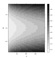
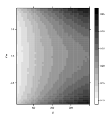
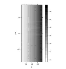
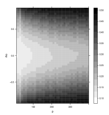
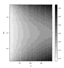
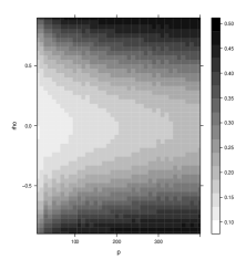
LDA for Case 1 Naive Bayes for Case 1 RLDA with $\lambda=0.5$ for Case 1 LDA for Case 2 Naive Bayes for Case 2 RLDA with $\lambda=0.5$ for Case 2 LDA for Case 3 Naive Bayes for Case 3 RLDA with $\lambda=0.5$ for Case 3

Figure 5: Heat maps of the error rates for LDA, Naive Bayes and RLDA with $\lambda=0.5$ where the horizontal is the data dimension $p$ ranging from 10 to 190 or 400 and the vertical is the correlation $\rho$ ranging from -0.9 to 0.9. The Bayes misclassification error rate is $10\%$.

5.3 RLDA and sparse LDA

In this part, we compare RLDA with the LPD (Cai and Liu, 2011) which is one of sparse LDA methods. The tuning parameters are chosen by 5-folds cross validation. We also include the RLDA where $\lambda_{n}$ is estimated by our method in Section 3.3 and the naive Bayes. In summary, we have four methods NB, LPD, RLDA-CV and RLDA. We control the sparsity level as

$$\Sigma^{-1}(\mu_{1}-\mu_{2})\propto(\mbox{rnorm(s)},0,\cdots,0);$$

with rnorm(s) represent $s$ random variables generated independently from $N(0,1)$, and in this study $s$ is increased from 5 to $p$. Figure 6 presents the simulation results. We observe that when $s$ is small, LPD is outstanding with the least error rates and the performance becomes poorer and poorer when $s$ increases, while RLDA and NB are robust to different $s$. Furthermore, we find out that the version with estimated tuning parameter is comparable to the one with cross validation. Overall, we claim that LPD is applicable to the sparse cases while RLDA is favorable to the dense cases.

$p=100$ $p=200$ $p=400$

Figure 6: Misclassification rates for naive Bayes, LPD and RLDA with cross validation and estimated $\lambda$. The horizontal is the number of non-zeros of $\Sigma^{-1}(\mu_{1}-\mu_{2})$.

6 Acknowledgments

We thank two reviewers, an associate editor, and the editor for their most helpful comments. Wang is partially supported by Shanghai Sailing Program 16YF1405700 and National Natural Science Foundation of China 11701367. Jiang is partially supported by the Early Career Scheme from Hong Kong Research Grants Council PolyU 253023/16P.

7 Appendix

Lemma 7.1.

Assuming $W_{m}\sim\mbox{Wishart}(I_{p},m)$ where $m>p+7$, for any non-random unit vector $e\in\mathbb{R}^{p}$, we have

$$E(e^{\mbox{\tiny{T}}}W_{m}^{-1}e)=\frac{1}{m-p-1},$$ (7.1)

$$E(e^{\mbox{\tiny{T}}}W_{m}^{-2}e)=\frac{m-1}{(m-p)(m-p-1)(m-p-3)},$$ (7.2)

and

$$E\{(e^{\mbox{\tiny{T}}}W_{m}^{-1}e)^{2}\}=\frac{1}{(m-p-1)(m-p-3)},$$ (7.3)

$$E\{(e^{\mbox{\tiny{T}}}W_{m}^{-2}e)^{2}\}=\frac{m^{2}}{(m-p)^{6}}\Big{\{}1+O\Big{(}\frac{1}{m-p}\Big{)}\Big{\}}.$$ (7.4)

Proof of Lemma 7.1: For any non-random orthogonal matrix $U$, we have

$$U^{\mbox{\tiny{T}}}W_{m}U\sim\mbox{Wishart}(I_{p},m),$$

and

$$e^{\mbox{\tiny{T}}}W_{m}^{-1}e\overset{d}{=}(Ue)^{\mbox{\tiny{T}}}W^{-1}_{m}Ue,~{}e^{\mbox{\tiny{T}}}W_{m}^{-2}e\overset{d}{=}(Ue)^{\mbox{\tiny{T}}}W^{-2}_{m}Ue.$$

Setting $Ue=(1,0,\cdots,0)^{\mbox{\tiny{T}}}$ yields

$$e^{\mbox{\tiny{T}}}W_{m}^{-1}e\overset{d}{=}(W_{m}^{-1})_{11},~{}e^{\mbox{\tiny{T}}}W_{m}^{-2}e\overset{d}{=}(W_{m}^{-2})_{11}=\sum_{i=1}^{p}(W_{m}^{-1})^{2}_{1i}.$$

Therefore, we can get the results (7.1)-(7.3) by von Rosen (1988) or the Proposition 2.1 of Cook and Forzani (2011). The order of (7.4) is derived based on Theorem 2 of Matsumoto (2012) and properties of the Weingarten function (Collins and Śniady, 2006) which involves lengthy and tedious calculations and is hence neglected.

Lemma 7.2.

Assuming $Y\sim N(0,I_{p})$ and $Y$ is independent with $S_{n}$, we have

$$\frac{1}{p}Y^{\mbox{\tiny{T}}}B_{n}(\lambda)Y\overset{p}{\to}R_{1}(\lambda),~{}~{}{\rm and}~{}~{}\frac{1}{p}Y^{\mbox{\tiny{T}}}B^{2}_{n}(\lambda)Y\overset{p}{\to}R_{2}(\lambda),$$

where $B_{n}(\lambda)$ and $R_{1}(\lambda),R_{2}(\lambda)$ are defined as in (3.1) and Theorem 3.1 respectively.

Proof of Lemma 7.2: Let $\|\cdot\|$ be the matrix operator norm. By direct calculations can have,

$$E\Big{\{}\frac{1}{p}Y^{\mbox{\tiny{T}}}B_{n}(\lambda)Y-\frac{1}{p}\mbox{tr}B_{n}(\lambda)\Big{\}} =0,$$

$$E\Big{\{}\frac{1}{p}Y^{\mbox{\tiny{T}}}B_{n}(\lambda)Y-\frac{1}{p}\mbox{tr}B_{n}(\lambda)\Big{\}}^{2} =E\frac{2}{p^{2}}\mbox{tr}B^{2}_{n}(\lambda)\leq\frac{2\|\Sigma\|^{2}}{\lambda^{2}p}\to 0,$$

$$E\Big{\{}\frac{1}{p}Y^{\mbox{\tiny{T}}}B^{2}_{n}(\lambda)Y-\frac{1}{p}\mbox{tr}B^{2}_{n}(\lambda)\Big{\}} =0,$$

$$E\Big{\{}\frac{1}{p}Y^{\mbox{\tiny{T}}}B^{2}_{n}(\lambda)Y-\frac{1}{p}\mbox{tr}B^{2}_{n}(\lambda)\Big{\}}^{2} =E\frac{2}{p^{2}}\mbox{tr}B^{4}_{n}(\lambda)\leq\frac{2\|\Sigma\|^{4}}{\lambda^{4}p}\to 0.$$

Here, we used the fact that

$$B_{n}(\lambda)=\Sigma^{\frac{1}{2}}(S_{n}+\lambda I)^{-1}\Sigma^{\frac{1}{2}}\overset{d}{=}(\frac{1}{n-2}W_{n}+\lambda\Sigma^{-1})^{-1},$$

where $W_{n}\sim\mbox{Wishart}(I_{p},n-2)$ is semidefinite and hence

$$\|B_{n}(\lambda)\|\leq\frac{1}{\lambda_{min}(\lambda\Sigma^{-1})}=\frac{\|\Sigma\|}{\lambda}.$$

Consequently we have,

$$\frac{1}{p}Y^{\mbox{\tiny{T}}}B_{n}(\lambda)Y=\frac{1}{p}\mbox{tr}B_{n}(\lambda)+o_{p}(1),~{}\frac{1}{p}Y^{\mbox{\tiny{T}}}B^{2}_{n}(\lambda)Y=\frac{1}{p}\mbox{tr}B^{2}_{n}(\lambda)+o_{p}(1).$$

Together with Theorem 2 of Wang et al. (2015) we have,

$$\frac{1}{p}\mbox{tr}B_{n}(\lambda)\overset{p}{\to}R_{1}(\lambda),~{}\frac{1}{p}\mbox{tr}B^{2}_{n}(\lambda)\overset{p}{\to}R_{2}(\lambda).$$ (7.5)

The proof is completed.

Lemma 7.3.

Under the conditions (C1)-(C3),

$$\mu^{\mbox{\tiny{T}}}B_{n}(\lambda)\mu\overset{p}{\to}\Delta^{2}H_{1}(\lambda),~{}\mu^{\mbox{\tiny{T}}}B^{2}_{n}(\lambda)\mu\overset{p}{\to}\Delta^{2}H_{2}(\lambda).$$

Proof of Lemma 7.3: By El Karoui and Holger (2011) we have,

$$\mu^{\mbox{\tiny{T}}}B_{n}(\lambda)\mu-\mu^{\mbox{\tiny{T}}}\Sigma^{\frac{1}{2}}(\gamma_{n}\Sigma+\lambda I_{p})^{-1}\Sigma^{\frac{1}{2}}\mu\overset{p}{\to}0,$$

$$\mu^{\mbox{\tiny{T}}}B^{2}_{n}(\lambda)\mu-(1+\epsilon_{n})\mu^{\mbox{\tiny{T}}}\Sigma^{\frac{1}{2}}(\gamma_{n}\Sigma+\lambda I_{p})^{-1}\Sigma(\gamma_{n}\Sigma+\lambda I_{p})^{-1}\Sigma^{\frac{1}{2}}\mu\overset{p}{\to}0,$$

where

$$\gamma_{n}=\frac{1}{1+\frac{1}{n-2}\mbox{tr}B_{n}(\lambda)},~{}\epsilon_{n}=\frac{\gamma_{n}^{2}}{n-2}\mbox{tr}B^{2}_{n}(\lambda).$$

From (7.5) we have

$$\gamma_{n}\overset{p}{\to}\frac{1}{1+yR_{1}(\lambda)}=1-y(1-\lambda m_{0}(-\lambda))\stackrel{{\scriptstyle\mbox{{\tiny def}}}}{{=}}\gamma,$$

$$\epsilon_{n}\overset{p}{\to}\frac{yR_{2}(\lambda)}{(1+yR_{1}(\lambda))^{2}}=\frac{y(1-\lambda m_{0}(-\lambda))}{1-y(1-\lambda m_{0}(-\lambda))}-\frac{y(\lambda m_{0}(-\lambda)-\lambda^{2}m^{\prime}_{0}(-\lambda))}{(1-y(1-\lambda m_{0}(-\lambda)))^{2}}\stackrel{{\scriptstyle\mbox{{\tiny def}}}}{{=}}\epsilon.$$

Consequently it can be routinely shown that

$$\mu^{\mbox{\tiny{T}}}B_{n}(\lambda)\mu-\mu^{\mbox{\tiny{T}}}\Sigma^{\frac{1}{2}}(\gamma\Sigma+\lambda I_{p})^{-1}\Sigma^{\frac{1}{2}}\mu\overset{p}{\to}0,$$

$$\mu^{\mbox{\tiny{T}}}B^{2}_{n}(\lambda)\mu-\frac{1+\epsilon}{\gamma^{2}}\Big{\{}\mu^{\mbox{\tiny{T}}}\Big{(}I_{p}+\frac{\lambda}{\gamma}\Sigma^{-1}\Big{)}^{-2}\mu\Big{\}}\overset{p}{\to}0,$$

By Condition (C3),

$$\mu^{\mbox{\tiny{T}}}\Sigma^{\frac{1}{2}}(\gamma\Sigma+\lambda I_{p})^{-1}\Sigma^{\frac{1}{2}}\mu=\gamma^{-1}\mu^{\mbox{\tiny{T}}}\Big{(}I_{p}+\frac{\lambda}{\gamma}\Sigma^{-1}\Big{)}^{-1}\mu\to\gamma^{-1}h_{1}\Big{(}\frac{\lambda}{\gamma}\Big{)}\Delta^{2},$$

and

$$\frac{1+\epsilon}{\gamma^{2}}\Big{\{}\mu^{\mbox{\tiny{T}}}\Big{(}I_{p}+\frac{\lambda}{\gamma}\Sigma^{-1}\Big{)}^{-2}\mu\Big{\}}\to\frac{1+\epsilon}{\gamma^{2}}h_{2}\Big{(}\frac{\lambda}{\gamma}\Big{)}\Delta^{2}.$$

The proof is completed.

7.1 Proof of Theorem 2.1

By the properties of Gaussian distributions,

$$\bar{X}_{1}\overset{d}{=}\frac{1}{\sqrt{n_{1}}}\Sigma^{\frac{1}{2}}Y_{1}+\mu_{1},~{}\bar{X}_{2}\overset{d}{=}\frac{1}{\sqrt{n_{2}}}\Sigma^{\frac{1}{2}}Y_{2}+\mu_{2},$$

where $Y_{1},Y_{2}\sim N(0,I_{p})$ and $Y_{1},Y_{2}$ are independent. We then have,

$$2\Big{(}\mu_{1}-\frac{\bar{X}_{1}+\bar{X}_{2}}{2}\Big{)}^{\mbox{\tiny{T}}}\Sigma^{-1}(\bar{X}_{1}-\bar{X}_{2}) =\Delta^{2}-\frac{2}{\sqrt{n_{2}}}\mu^{\mbox{\tiny{T}}}Y_{2}+\frac{1}{n_{2}}Y_{2}^{\mbox{\tiny{T}}}Y_{2}-\frac{1}{n_{1}}Y_{1}^{\mbox{\tiny{T}}}Y_{1}$$

$$\overset{p}{\to}\Delta^{2}+y_{2}-y_{1},$$

and

$$-2\Big{(}\mu_{2}-\frac{\bar{X}_{1}+\bar{X}_{2}}{2}\Big{)}^{\mbox{\tiny{T}}}\Sigma^{-1}(\bar{X}_{1}-\bar{X}_{2}) =\Delta^{2}+\frac{2}{\sqrt{n_{1}}}\mu^{\mbox{\tiny{T}}}Y_{1}+\frac{1}{n_{1}}Y_{1}^{\mbox{\tiny{T}}}Y_{1}-\frac{1}{n_{2}}Y_{2}^{\mbox{\tiny{T}}}Y_{2}$$

$$\overset{p}{\to}\Delta^{2}+y_{1}-y_{2},$$

where $\mu$ is defined as in (3.1). For the denominator,

$$(\bar{X}_{1}-\bar{X}_{2})^{\mbox{\tiny{T}}}\Sigma^{-1}(\bar{X}_{1}-\bar{X}_{2})$$

$$= \Delta^{2}+\frac{1}{n_{1}}Y^{\mbox{\tiny{T}}}_{1}Y_{1}+\frac{1}{n_{2}}Y^{\mbox{\tiny{T}}}_{2}Y_{2}+2\mu^{\mbox{\tiny{T}}}\Big{(}\frac{1}{\sqrt{n_{1}}}Y_{1}-\frac{1}{\sqrt{n}_{2}}Y_{2}\Big{)}-\frac{2}{\sqrt{n_{1}n_{2}}}Y^{\mbox{\tiny{T}}}_{1}Y_{2}$$

$$\overset{p}{\to} \Delta^{2}+y_{1}+y_{2}.$$

By the Slutsky’s theorem and the continuous mapping theorem, the proof is completed.

7.2 Proof of Theorem 2.2

Write

$$S_{n}\overset{d}{=}\frac{1}{n-2}\Sigma^{\frac{1}{2}}W_{n}\Sigma^{\frac{1}{2}},$$

where $W_{n}\sim\mbox{Wishart}(I_{p},n-2)$. Then

$$\mbox{R}_{\text{LDA2}}\overset{d}{=}\Phi\Big{(}\frac{-\mu^{\mbox{\tiny{T}}}W_{n}^{-1}\mu}{2\sqrt{\mu^{\mbox{\tiny{T}}}W_{n}^{-2}\mu}}\Big{)}.$$

By Lemma 7.1, when $p/n\to y\in(0,1)$, we have

$$nE\mu^{\mbox{\tiny{T}}}W_{n}^{-1}\mu=\frac{n\Delta^{2}}{n-p-3}\to\frac{\Delta^{2}}{1-y},$$

$$n^{2}E\mu^{\mbox{\tiny{T}}}W_{n}^{-2}\mu=\frac{n^{2}(n-3)\Delta^{2}}{(n-p-2)(n-p-3)(n-p-5)}\to\frac{\Delta^{2}}{(1-y)^{3}},$$

and

$$Var(n\mu^{\mbox{\tiny{T}}}W_{n}^{-1}\mu)=\Delta^{4}\Big{\{}\frac{n^{2}}{(n-p-3)(n-p-5)}-\frac{n^{2}}{(n-p-3)^{2}}\Big{\}}\to 0,$$

$$Var(n^{2}\mu^{\mbox{\tiny{T}}}W_{n}^{-2}\mu)=\Delta^{4}\Big{\{}\frac{n^{6}}{(n-p)^{6}}(1+o(1))-\frac{n^{4}(n-3)^{2}}{(n-p-2)^{2}(n-p-3)^{2}(n-p-5)^{2}}\Big{\}}\to 0.$$

Therefore,

$$n\mu^{\mbox{\tiny{T}}}W_{n}^{-1}\mu\overset{p}{\to}\frac{\Delta^{2}}{1-y},~{}n^{2}\mu^{\mbox{\tiny{T}}}W_{n}^{-2}\mu\overset{p}{\to}\frac{\Delta^{2}}{(1-y)^{3}}.$$

The proof is completed.

7.3 Proof of Theorem 2.3

We have

$$\bar{X}_{1}\overset{d}{=}\frac{1}{\sqrt{n_{1}}}\Sigma^{\frac{1}{2}}Y_{1}+\mu_{1},~{}\bar{X}_{2}\overset{d}{=}\frac{1}{\sqrt{n_{2}}}\Sigma^{\frac{1}{2}}Y_{2}+\mu_{2},S_{n}\overset{d}{=}\frac{1}{n-2}\Sigma^{\frac{1}{2}}W_{n}\Sigma^{\frac{1}{2}},$$

where $Y_{1},Y_{2}\sim N(0,I_{p}),~{}W_{n}\sim\mbox{Wishart}(I_{p},n-2)$ and $Y_{1},Y_{2},W_{n}$ are independent. Then

$$-\Big{(}\mu_{1}-\frac{\bar{X}_{1}+\bar{X}_{2}}{2}\Big{)}^{\mbox{\tiny{T}}}S_{n}^{-1}(\bar{X}_{1}-\bar{X}_{2})$$

$$\overset{d}{=} -\frac{n-2}{2}\Big{(}\mu-\frac{1}{\sqrt{n_{1}}}Y_{1}-\frac{1}{\sqrt{n_{2}}}Y_{2}\Big{)}^{\mbox{\tiny{T}}}W_{n}^{-1}\Big{(}\mu+\frac{1}{\sqrt{n_{1}}}Y_{1}-\frac{1}{\sqrt{n_{2}}}Y_{2}\Big{)}$$

$$= -\frac{n-2}{2}\Big{(}\mu-\frac{1}{\sqrt{n_{2}}}Y_{2}\Big{)}^{\mbox{\tiny{T}}}W_{n}^{-1}\Big{(}\mu-\frac{1}{\sqrt{n_{2}}}Y_{2}\Big{)}+\frac{n-2}{2n_{1}}Y_{1}^{\mbox{\tiny{T}}}W_{n}^{-1}Y_{1}.$$

By Lemma 7.1, we have,

$$EY_{1}^{\mbox{\tiny{T}}}W_{n}^{-1}Y_{1}=\frac{1}{n-p-3}EY_{1}^{\mbox{\tiny{T}}}Y_{1}=\frac{p}{n-p-3}\to\frac{y}{1-y},$$

and

$$Var(Y_{1}^{\mbox{\tiny{T}}}W_{n}^{-1}Y_{1})= E(Y_{1}^{\mbox{\tiny{T}}}W_{n}^{-1}Y_{1})^{2}-(EY_{1}^{\mbox{\tiny{T}}}W_{n}^{-1}Y_{1})^{2}$$

$$= \frac{E(Y_{1}^{\mbox{\tiny{T}}}Y_{1})^{2}}{(n-p-3)(n-p-5)}-\frac{p^{2}}{(n-p-3)^{2}}$$

$$= \frac{p^{2}+2p}{(n-p-3)(n-p-5)}-\frac{p^{2}}{(n-p-3)^{2}}\to 0.$$

Similarly,

$$E(n-2)\Big{(}\mu-\frac{1}{\sqrt{n_{2}}}Y_{2}\Big{)}^{\mbox{\tiny{T}}}W_{n}^{-1}\Big{(}\mu-\frac{1}{\sqrt{n_{2}}}Y_{2}\Big{)}$$

$$= \frac{n-2}{n-p-3}E\Big{(}\mu-\frac{1}{\sqrt{n_{2}}}Y_{2}\Big{)}^{\mbox{\tiny{T}}}\Big{(}\mu-\frac{1}{\sqrt{n_{2}}}Y_{2}\Big{)}$$

$$= \frac{n-2}{n-p-3}\Big{(}\Delta^{2}+\frac{p}{n_{2}}\Big{)}\to\frac{1}{1-y}(\Delta^{2}+y_{2}),$$

and

$$Var\Big{\{}(n-2)\Big{(}\mu-\frac{1}{\sqrt{n_{2}}}Y_{2}\Big{)}^{\mbox{\tiny{T}}}W_{n}^{-1}\Big{(}\mu-\frac{1}{\sqrt{n_{2}}}Y_{2}\Big{)}\Big{\}}$$

$$= \frac{(n-2)^{2}E\{\big{(}\mu-\frac{1}{\sqrt{n_{2}}}Y_{2}\big{)}^{\mbox{\tiny{T}}}\big{(}\mu-\frac{1}{\sqrt{n_{2}}}Y_{2}\big{)}\}^{2}}{(n-p-3)(n-p-5)}-\frac{(n-2)^{2}\big{(}\Delta^{2}+\frac{p}{n_{2}}\big{)}^{2}}{(n-p-3)^{2}}$$

$$= \frac{(n-2)^{2}\big{(}\Delta^{4}+\frac{(2p+4)\Delta^{2}}{n_{2}}+\frac{p^{2}+2p}{n_{2}^{2}}\big{)}}{(n-p-3)(n-p-5)}-\frac{(n-2)^{2}\big{(}\Delta^{2}+\frac{p}{n_{2}}\big{)}^{2}}{(n-p-3)^{2}}\to 0.$$

Thus,

$$-\Big{(}\mu_{1}-\frac{\bar{X}_{1}+\bar{X}_{2}}{2}\Big{)}^{\mbox{\tiny{T}}}S_{n}^{-1}(\bar{X}_{1}-\bar{X}_{2})$$

$$\overset{d}{=} -\frac{n-2}{2}\Big{(}\mu-\frac{1}{\sqrt{n_{2}}}Y_{2}\Big{)}^{\mbox{\tiny{T}}}W_{n}^{-1}\Big{(}\mu-\frac{1}{\sqrt{n_{2}}}Y_{2}\Big{)}+\frac{n-2}{2n_{1}}Y_{1}^{\mbox{\tiny{T}}}W_{n}^{-1}Y_{1}$$

$$\overset{p}{\to} -\frac{1}{2(1-y)}(\Delta^{2}+y_{2})+\frac{y_{1}}{2y}\frac{y}{1-y}=-\frac{\Delta^{2}-y_{1}+y_{2}}{2(1-y)},$$ (7.6)

and by similar arguments, we have

$$\Big{(}\mu_{2}-\frac{\bar{X}_{1}+\bar{X}_{2}}{2}\Big{)}^{\mbox{\tiny{T}}}S_{n}^{-1}(\bar{X}_{1}-\bar{X}_{2})$$

$$\overset{d}{=} -\frac{n-2}{2}\Big{(}\mu+\frac{1}{\sqrt{n_{1}}}Y_{1}\Big{)}^{\mbox{\tiny{T}}}W_{n}^{-1}\Big{(}\mu+\frac{1}{\sqrt{n_{1}}}Y_{1}\Big{)}+\frac{n-2}{2n_{2}}Y_{2}^{\mbox{\tiny{T}}}W_{n}^{-1}Y_{2}$$

$$\overset{p}{\to} -\frac{\Delta^{2}+y_{1}-y_{2}}{2(1-y)}.$$ (7.7)

For the denominator, we have

$$(\bar{X}_{1}-\bar{X}_{2})^{\mbox{\tiny{T}}}S_{n}^{-1}\Sigma S_{n}^{-1}(\bar{X}_{1}-\bar{X}_{2})$$

$$\overset{d}{=} (n-2)^{2}\Big{(}\mu+\frac{1}{\sqrt{n_{1}}}Y_{1}-\frac{1}{\sqrt{n_{2}}}Y_{2}\Big{)}^{\mbox{\tiny{T}}}W_{n}^{-2}\Big{(}\mu+\frac{1}{\sqrt{n_{1}}}Y_{1}-\frac{1}{\sqrt{n_{2}}}Y_{2}\Big{)}.$$

By Lemma 7.1, we have,

$$E(n-2)^{2}\Big{(}\mu+\frac{1}{\sqrt{n_{1}}}Y_{1}-\frac{1}{\sqrt{n_{2}}}Y_{2}\Big{)}^{\mbox{\tiny{T}}}W_{n}^{-2}\Big{(}\mu+\frac{1}{\sqrt{n_{1}}}Y_{1}-\frac{1}{\sqrt{n_{2}}}Y_{2}\Big{)}$$

$$= \frac{(n-2)^{2}(n-3)E\big{(}\mu+\frac{1}{\sqrt{n_{1}}}Y_{1}-\frac{1}{\sqrt{n_{2}}}Y_{2}\big{)}^{\mbox{\tiny{T}}}\big{(}\mu+\frac{1}{\sqrt{n_{1}}}Y_{1}-\frac{1}{\sqrt{n_{2}}}Y_{2}\big{)}}{(n-p-2)(n-p-3)(n-p-5)}$$

$$= \frac{(n-2)^{2}(n-3)\big{(}\Delta^{2}+\frac{p}{n_{1}}+\frac{p}{n_{2}}\big{)}}{(n-p-2)(n-p-3)(n-p-5)}\to\frac{\Delta^{2}+y_{1}+y_{2}}{(1-y)^{3}},$$

and

$$E\Big{\{}(n-2)^{2}\Big{(}\mu+\frac{1}{\sqrt{n_{1}}}Y_{1}-\frac{1}{\sqrt{n_{2}}}Y_{2}\Big{)}^{\mbox{\tiny{T}}}W_{n}^{-2}\Big{(}\mu+\frac{1}{\sqrt{n_{1}}}Y_{1}-\frac{1}{\sqrt{n_{2}}}Y_{2}\Big{)}\Big{\}}^{2}$$

$$= \Big{\{}\frac{n^{6}}{(n-p)^{6}}+o(1)\Big{\}}E\Big{\{}\Big{(}\mu+\frac{1}{\sqrt{n_{1}}}Y_{1}-\frac{1}{\sqrt{n_{2}}}Y_{2}\Big{)}^{\mbox{\tiny{T}}}\Big{(}\mu+\frac{1}{\sqrt{n_{1}}}Y_{1}-\frac{1}{\sqrt{n_{2}}}Y_{2}\Big{)}\Big{\}}^{2}$$

$$= \Big{\{}\frac{n^{6}}{(n-p)^{6}}+o(1)\Big{\}}\Big{\{}\Big{(}\Delta^{2}+\frac{p}{n_{1}}+\frac{p}{n_{2}}\Big{)}^{2}+o(1)\Big{\}}\to\frac{(\Delta^{2}+y_{1}+y_{2})^{2}}{(1-y)^{6}}.$$

Thus,

$$(\bar{X}_{1}-\bar{X}_{2})^{\mbox{\tiny{T}}}S_{n}^{-1}\Sigma S_{n}^{-1}(\bar{X}_{1}-\bar{X}_{2})\overset{p}{\to}\frac{\Delta^{2}+y_{1}+y_{2}}{(1-y)^{3}}.$$ (7.8)

Combing (7.6), (7.7) and (7.8), the proof is completed.

7.4 Proof of Proposition 2.1

With some simple calculation it can be shown that the misclassification rate of $\delta_{\rm LDA}^{c}(X)$ is

$$\mbox{R}_{\text{LDA}}^{c}=\frac{1}{2}\sum_{j=1}^{2}\Phi\left(\frac{(-1)^{j}\big{[}(\mu_{j}-\frac{\bar{X}_{1}+\bar{X}_{2}}{2})^{\mbox{\tiny{T}}}S_{n}^{-1}(\bar{X}_{1}-\bar{X}_{2})+\alpha\big{]}}{\sqrt{(\bar{X}_{1}-\bar{X}_{2})^{\mbox{\tiny{T}}}S_{n}^{-1}\Sigma S_{n}^{-1}(\bar{X}_{1}-\bar{X}_{2})}}\right).$$

where $\alpha=\frac{n-2}{n-p-3}\big{(}\frac{p}{2n_{1}}-\frac{p}{2n_{2}}\big{)}$. Note that from (7.6) and the fact that $\alpha\rightarrow\frac{y_{1}-y_{2}}{2(1-y)}$, we have

$$-\bigg{[}\Big{(}\mu_{1}-\frac{\bar{X}_{1}+\bar{X}_{2}}{2}\Big{)}^{\mbox{\tiny{T}}}S_{n}^{-1}(\bar{X}_{1}-\bar{X}_{2})+\alpha\bigg{]} \overset{p}{\to} -\frac{\Delta^{2}-y_{1}+y_{2}}{2(1-y)}-\frac{y_{1}-y_{2}}{2(1-y)}$$

$$= -\frac{\Delta^{2}}{2(1-y)}.$$

Similarly, by (7.7) we have

$$\bigg{[}\Big{(}\mu_{2}-\frac{\bar{X}_{1}+\bar{X}_{2}}{2}\Big{)}^{\mbox{\tiny{T}}}S_{n}^{-1}(\bar{X}_{1}-\bar{X}_{2})+\alpha\bigg{]} \overset{p}{\to} -\frac{\Delta^{2}}{2(1-y)}.$$

Combining with (7.8) we have

$$\mbox{R}_{\text{LDA}}^{c} \overset{p}{\to} \Phi\left(-\frac{\Delta^{2}}{2(1-y)}\frac{(1-y)^{3/2}}{\sqrt{\Delta^{2}+y_{1}+y_{2}}}\right)$$

$$= \Phi\left(-\frac{\Delta^{2}}{2\sqrt{\Delta^{2}+y_{1}+y_{2}}}\sqrt{1-y}\right).$$

7.5 Proof of Theorem 3.1

Write

$$T_{1n}=(2\mu_{1}-\bar{X}_{1}-\bar{X}_{2})^{\mbox{\tiny{T}}}(S_{n}+\lambda I_{p})^{-1}(\bar{X}_{1}-\bar{X}_{2}),$$

$$T_{2n}=-(2\mu_{2}-\bar{X}_{1}-\bar{X}_{2})^{\mbox{\tiny{T}}}(S_{n}+\lambda I_{p})^{-1}(\bar{X}_{1}-\bar{X}_{2}),$$

$$T_{3n}=(\bar{X}_{1}-\bar{X}_{2})^{\mbox{\tiny{T}}}(S_{n}+\lambda I_{p})^{-1}\Sigma(S_{n}+\lambda I_{p})^{-1}(\bar{X}_{1}-\bar{X}_{2}).$$

Since

$$\bar{X}_{1}\overset{d}{=}\frac{1}{\sqrt{n_{1}}}\Sigma^{\frac{1}{2}}Y_{1}+\mu_{1},~{}\bar{X}_{2}\overset{d}{=}\frac{1}{\sqrt{n_{2}}}\Sigma^{\frac{1}{2}}Y_{2}+\mu_{2},$$

where $Y_{1},Y_{2}\sim N(0,I_{p})$ and $Y_{1},Y_{2},S_{n}$ are independent, we have

$$T_{1n}\overset{d}{=} \mu^{\mbox{\tiny{T}}}B_{n}(\lambda)\mu-\frac{2}{\sqrt{n_{2}}}\mu^{\mbox{\tiny{T}}}B_{n}(\lambda)Y_{2}+\frac{1}{n_{2}}Y_{2}^{\mbox{\tiny{T}}}B_{n}(\lambda)Y_{2}-\frac{1}{n_{1}}Y_{1}^{\mbox{\tiny{T}}}B_{n}(\lambda)Y_{1},$$

$$T_{2n}\overset{d}{=} \mu^{\mbox{\tiny{T}}}B_{n}(\lambda)\mu+\frac{2}{\sqrt{n_{1}}}\mu^{\mbox{\tiny{T}}}B_{n}(\lambda)Y_{1}+\frac{1}{n_{1}}Y_{1}^{\mbox{\tiny{T}}}B_{n}(\lambda)Y_{1}-\frac{1}{n_{2}}Y_{2}^{\mbox{\tiny{T}}}B_{n}(\lambda)Y_{2},$$

$$T_{3n}\overset{d}{=} \Big{(}\mu+\frac{1}{\sqrt{n_{1}}}Y_{1}-\frac{1}{\sqrt{n_{2}}}Y_{2}\Big{)}^{\mbox{\tiny{T}}}B^{2}_{n}(\lambda)\Big{(}\mu+\frac{1}{\sqrt{n_{1}}}Y_{1}-\frac{1}{\sqrt{n_{2}}}Y_{2}\Big{)}$$

$$\overset{d}{=} \mu^{\mbox{\tiny{T}}}B^{2}_{n}(\lambda)\mu+2\sqrt{\frac{1}{n_{1}}+\frac{1}{n_{2}}}\mu^{\mbox{\tiny{T}}}B^{2}_{n}(\lambda)Y_{1}+\Big{(}\frac{1}{n_{1}}+\frac{1}{n_{2}}\Big{)}Y_{1}^{\mbox{\tiny{T}}}B^{2}_{n}(\lambda)Y_{1}.$$

For the leading terms, by Lemmas 7.2 and 7.3,

$$\frac{1}{n_{j}}Y_{j}^{\mbox{\tiny{T}}}B_{n}(\lambda)Y_{j}\overset{p}{\to}y_{j}R_{1}(\lambda),~{}j=1,2$$

$$\Big{(}\frac{1}{n_{1}}+\frac{1}{n_{2}}\Big{)}Y_{1}^{\mbox{\tiny{T}}}B^{2}_{n}(\lambda)Y_{1}\overset{p}{\to}(y_{1}+y_{2})R_{2}(\lambda)$$

$$\mu^{\mbox{\tiny{T}}}B_{n}(\lambda)\mu\overset{p}{\to}H_{1}(\lambda)\Delta^{2},~{}\mu^{\mbox{\tiny{T}}}B^{2}_{n}(\lambda)\mu\overset{p}{\to}H_{2}(\lambda)\Delta^{2}.$$

For the cross sectional terms,

$$E\Big{\{}\frac{1}{\sqrt{n_{j}}}\mu^{\mbox{\tiny{T}}}B_{n}(\lambda)Y_{j}\Big{\}}^{2}=\frac{1}{n_{j}}E\mu^{\mbox{\tiny{T}}}B^{2}_{n}(\lambda)\mu\leq\frac{\Delta^{2}\|\Sigma\|^{2}}{n_{j}\lambda^{2}}\to 0,$$

and similarly,

$$E\Big{\{}\frac{1}{\sqrt{n}}\mu^{\mbox{\tiny{T}}}B^{2}_{n}(\lambda)Y_{1}\Big{\}}^{2}=\frac{1}{n}E\mu^{\mbox{\tiny{T}}}B^{4}_{n}(\lambda)\mu\leq\frac{\Delta^{2}\|\Sigma\|^{4}}{n_{j}\lambda^{4}}\to 0.$$

Thus,

$$\frac{1}{\sqrt{n_{1}}}\mu^{\mbox{\tiny{T}}}B_{n}(\lambda)Y_{1},\frac{1}{\sqrt{n_{2}}}\mu^{\mbox{\tiny{T}}}B_{n}(\lambda)Y_{2},\sqrt{\frac{1}{n_{1}}+\frac{1}{n_{2}}}\mu^{\mbox{\tiny{T}}}B^{2}_{n}(\lambda)Y_{1}\overset{p}{\to}0.$$

Above all,

$$T_{1n}\overset{p}{\to}H_{1}(\lambda)\Delta^{2}+(y_{2}-y_{1})R_{1}(\lambda),~{}T_{2n}\overset{p}{\to}H_{1}(\lambda)+(y_{1}-y_{2})R_{1}(\lambda),$$

$$T_{3n}\overset{p}{\to}H_{2}(\lambda)\Delta^{2}+(y_{1}+y_{2})R_{2}(\lambda).$$

By the continuous mapping theorem, the proof is completed.

7.6 Proof of Proposition 3.1

When

$$h_{1}(t)=\int\frac{x}{x+t}dH(x),~{}h_{2}(t)=\int\frac{x}{(x+t)^{2}}dH(x),$$

by the definitions of $H_{1}(\lambda)$ and $H_{2}(\lambda)$, we have

$$H_{1}(\lambda)= (1+yR_{1}(\lambda))h_{1}(\lambda(1+yR_{1}(\lambda)))=\int\frac{1}{\frac{\lambda}{x}+\frac{1}{1+yR_{1}(\lambda)}}dH(x),$$

and

$$H_{2}(\lambda)= \{(1+yR_{1}(\lambda))^{2}+yR_{2}(\lambda)\}\int\frac{x^{2}}{(x+\lambda(1+yR_{1}(\lambda))^{2})}dH(x)$$

$$= \int\frac{1+\frac{yR_{2}(\lambda)}{(1+yR_{1}(\lambda))^{2}}}{(\frac{\lambda}{x}+\frac{1}{1+yR_{1}(\lambda)})^{2}}dH(x).$$

Compared with Lemma 2 of Wang et al. (2015), $H_{1}(\lambda)=R_{1}(\lambda)$ and $H_{2}(\lambda)=R_{2}(\lambda)$. The convergence of misclassification rate is a direct conclusion of Theorem 3.1. The proof is completed.

References

- Anderson (2003) {bbook}[author] \bauthor\bsnmAnderson, \bfnmTW\binitsT. (\byear2003). \btitleAn introduction to multivariate statistical analysis. \bpublisherWiley Series in Probability and Statistics. \endbibitem
- Aoshima and Yata (2014) {barticle}[author] \bauthor\bsnmAoshima, \bfnmMakoto\binitsM. and \bauthor\bsnmYata, \bfnmKazuyoshi\binitsK. (\byear2014). \btitleA distance-based, misclassification rate adjusted classifier for multiclass, high-dimensional data. \bjournalAnnals of the Institute of Statistical Mathematics \bvolume66 \bpages983–1010. \endbibitem
- Bai, Liu and Wong (2009) {barticle}[author] \bauthor\bsnmBai, \bfnmZhidong\binitsZ., \bauthor\bsnmLiu, \bfnmHuixia\binitsH. and \bauthor\bsnmWong, \bfnmWing-Keung\binitsW.-K. (\byear2009). \btitleEnhancement of the applicability of Markowitz’s portfolio optimization by utilizing random matrix theory. \bjournalMathematical Finance \bvolume19 \bpages639–667. \endbibitem
- Bai, Liu and Wong (2011) {barticle}[author] \bauthor\bsnmBai, \bfnmZD\binitsZ., \bauthor\bsnmLiu, \bfnmHX\binitsH. and \bauthor\bsnmWong, \bfnmWK\binitsW. (\byear2011). \btitleAsymptotic properties of eigenmatrices of a large sample covariance matrix. \bjournalThe Annals of Applied Probability \bvolume21 \bpages1994–2015. \endbibitem
- Bai, Miao and Pan (2007) {barticle}[author] \bauthor\bsnmBai, \bfnmZD\binitsZ., \bauthor\bsnmMiao, \bfnmBQ\binitsB. and \bauthor\bsnmPan, \bfnmGM\binitsG. (\byear2007). \btitleOn asymptotics of eigenvectors of large sample covariance matrix. \bjournalAnnals of Probability \bvolume35 \bpages1532–1572. \endbibitem
- Bai and Saranadasa (1996) {barticle}[author] \bauthor\bsnmBai, \bfnmZhidong\binitsZ. and \bauthor\bsnmSaranadasa, \bfnmHewa\binitsH. (\byear1996). \btitleEffect of high dimension: by an example of a two sample problem. \bjournalStatistica Sinica \bvolume2 \bpages311–329. \endbibitem
- Bai and Silverstein (2010) {bbook}[author] \bauthor\bsnmBai, \bfnmZhidong\binitsZ. and \bauthor\bsnmSilverstein, \bfnmJack W\binitsJ. W. (\byear2010). \btitleSpectral analysis of large dimensional random matrices. \bpublisherSpringer. \endbibitem
- Bickel and Levina (2004) {barticle}[author] \bauthor\bsnmBickel, \bfnmP. J.\binitsP. J. and \bauthor\bsnmLevina, \bfnmE.\binitsE. (\byear2004). \btitleSome theory for Fisher’s linear discriminant function,naive Bayes’, and some alternatives when there are many more variables than observations. \bjournalBernoulli \bvolume10 \bpages989–1010. \endbibitem
- Bühlmann (2013) {barticle}[author] \bauthor\bsnmBühlmann, \bfnmPeter\binitsP. (\byear2013). \btitleStatistical significance in high-dimensional linear models. \bjournalBernoulli \bvolume19 \bpages1212–1242. \endbibitem
- Cai and Liu (2011) {barticle}[author] \bauthor\bsnmCai, \bfnmTony\binitsT. and \bauthor\bsnmLiu, \bfnmWeidong\binitsW. (\byear2011). \btitleA direct estimation approach to sparse linear discriminant analysis. \bjournalJournal of the American Statistical Association \bvolume106 \bpages1566–1577. \endbibitem
- Cai, Liu and Luo (2011) {barticle}[author] \bauthor\bsnmCai, \bfnmTony\binitsT., \bauthor\bsnmLiu, \bfnmWeidong\binitsW. and \bauthor\bsnmLuo, \bfnmXi\binitsX. (\byear2011). \btitleA constrained minimization approach to sparse precision matrix estimation. \bjournalJournal of the American Statistical Association \bvolume106 \bpages594–607. \endbibitem
- Cai, Liu and Xia (2014) {barticle}[author] \bauthor\bsnmCai, \bfnmTony\binitsT., \bauthor\bsnmLiu, \bfnmWeidong\binitsW. and \bauthor\bsnmXia, \bfnmYin\binitsY. (\byear2014). \btitleTwo-sample test of high dimensional means under dependence. \bjournalJournal of the Royal Statistical Society, Series B \bvolume76 \bpages349–372. \endbibitem
- Chan and Hall (2009) {barticle}[author] \bauthor\bsnmChan, \bfnmYao-Ban\binitsY.-B. and \bauthor\bsnmHall, \bfnmPeter\binitsP. (\byear2009). \btitleScale adjustments for classifiers in high-dimensional, low sample size settings. \bjournalBiometrika \bvolume96 \bpages469–478. \endbibitem
- Chen et al. (2011) {barticle}[author] \bauthor\bsnmChen, \bfnmLin S\binitsL. S., \bauthor\bsnmPaul, \bfnmDebashis\binitsD., \bauthor\bsnmPrentice, \bfnmRoss L\binitsR. L. and \bauthor\bsnmWang, \bfnmPei\binitsP. (\byear2011). \btitleA regularized Hotelling’s test for pathway analysis in proteomic studies. \bjournalJournal of the American Statistical Association \bvolume106. \endbibitem
- Cheng (2004) {barticle}[author] \bauthor\bsnmCheng, \bfnmYu\binitsY. (\byear2004). \btitleAsymptotic probabilities of misclassification of two discriminant functions in cases of high dimensional data. \bjournalStatistics & Probability Letters \bvolume67 \bpages9–17. \endbibitem
- Collins and Śniady (2006) {barticle}[author] \bauthor\bsnmCollins, \bfnmBenoît\binitsB. and \bauthor\bsnmŚniady, \bfnmPiotr\binitsP. (\byear2006). \btitleIntegration with respect to the Haar measure on unitary, orthogonal and symplectic group. \bjournalCommunications in Mathematical Physics \bvolume264 \bpages773–795. \endbibitem
- Cook and Forzani (2011) {barticle}[author] \bauthor\bsnmCook, \bfnmR Dennis\binitsR. D. and \bauthor\bsnmForzani, \bfnmLiliana\binitsL. (\byear2011). \btitleOn the mean and variance of the generalized inverse of a singular Wishart matrix. \bjournalElectronic Journal of Statistics \bvolume5 \bpages146–158. \endbibitem
- Dobriban and Wager (2018) {barticle}[author] \bauthor\bsnmDobriban, \bfnmEdgar\binitsE. and \bauthor\bsnmWager, \bfnmStefan\binitsS. (\byear2018). \btitleHigh-dimensional asymptotics of prediction: Ridge regression and classification. \bjournalAnnals of Statistics \bvolume46 \bpages247–279. \endbibitem
- Dudoit, Fridlyand and Speed (2002) {barticle}[author] \bauthor\bsnmDudoit, \bfnmSandrine\binitsS., \bauthor\bsnmFridlyand, \bfnmJane\binitsJ. and \bauthor\bsnmSpeed, \bfnmTerence P\binitsT. P. (\byear2002). \btitleComparison of discrimination methods for the classification of tumors using gene expression data. \bjournalJournal of the American Statistical Association \bvolume97 \bpages77–87. \endbibitem
- El Karoui (2008) {barticle}[author] \bauthor\bsnmEl Karoui, \bfnmNoureddine\binitsN. (\byear2008). \btitleSpectrum estimation for large dimensional covariance matrices using random matrix theory. \bjournalAnnals of Statistics \bvolume36 \bpages2757–2790. \endbibitem
- El Karoui (2010) {barticle}[author] \bauthor\bsnmEl Karoui, \bfnmNoureddine\binitsN. (\byear2010). \btitleHigh-dimensionality effects in the Markowitz problem and other quadratic programs with linear constraints: Risk underestimation. \bjournalAnnals of Statistics \bvolume38 \bpages3487–3566. \endbibitem
- El Karoui and Holger (2011) {barticle}[author] \bauthor\bsnmEl Karoui, \bfnmNoureddine\binitsN. and \bauthor\bsnmHolger, \bfnmKösters\binitsK. (\byear2011). \btitleGeometric sensitivity of random matrix results: consequences for shrinkage estimators of covariance and related statistical methods. \bjournalarXiv:1105.1404. \endbibitem
- Fan, Feng and Tong (2012) {barticle}[author] \bauthor\bsnmFan, \bfnmJianqing\binitsJ., \bauthor\bsnmFeng, \bfnmYang\binitsY. and \bauthor\bsnmTong, \bfnmXin\binitsX. (\byear2012). \btitleA road to classification in high dimensional space: the regularized optimal affine discriminant. \bjournalJournal of the Royal Statistical Society, Series B \bvolume74 \bpages745–771. \endbibitem
- Friedman (1989) {barticle}[author] \bauthor\bsnmFriedman, \bfnmJerome H\binitsJ. H. (\byear1989). \btitleRegularized discriminant analysis. \bjournalJournal of the American Statistical Association \bvolume84 \bpages165–175. \endbibitem
- Guo, Hastie and Tibshirani (2007) {barticle}[author] \bauthor\bsnmGuo, \bfnmYaqian\binitsY., \bauthor\bsnmHastie, \bfnmTrevor\binitsT. and \bauthor\bsnmTibshirani, \bfnmRobert\binitsR. (\byear2007). \btitleRegularized linear discriminant analysis and its application in microarrays. \bjournalBiostatistics \bvolume8 \bpages86–100. \endbibitem
- Hand (2006) {barticle}[author] \bauthor\bsnmHand, \bfnmDavid\binitsD. (\byear2006). \btitleClassifier technology and the illusion of progress. \bjournalStatistical Science \bvolume21 \bpages1–14. \endbibitem
- Huang, Tong and Zhao (2010) {barticle}[author] \bauthor\bsnmHuang, \bfnmSong\binitsS., \bauthor\bsnmTong, \bfnmTiejun\binitsT. and \bauthor\bsnmZhao, \bfnmHongyu\binitsH. (\byear2010). \btitleBias-Corrected Diagonal Discriminant Rules for High-Dimensional Classification. \bjournalBiometrics \bvolume66 \bpages1096–1106. \endbibitem
- Jiang and Yang (2013) {barticle}[author] \bauthor\bsnmJiang, \bfnmTiefeng\binitsT. and \bauthor\bsnmYang, \bfnmFan\binitsF. (\byear2013). \btitleCentral limit theorems for classical likelihood ratio tests for high-dimensional normal distributions. \bjournalAnnals of Statistics \bvolume41 \bpages2029–2074. \endbibitem
- Kubokawa and Srivastava (2008) {barticle}[author] \bauthor\bsnmKubokawa, \bfnmTatsuya\binitsT. and \bauthor\bsnmSrivastava, \bfnmM. S.\binitsM. S. (\byear2008). \btitleEstimation of the precision matrix of a singular Wishart distribution and its application in high-dimensional data. \bjournalJournal of Multivariate Analysis \bvolume99 \bpages1906–1928. \endbibitem
- Ledoit and Péché (2011) {barticle}[author] \bauthor\bsnmLedoit, \bfnmOlivier\binitsO. and \bauthor\bsnmPéché, \bfnmSandrine\binitsS. (\byear2011). \btitleEigenvectors of some large sample covariance matrix ensembles. \bjournalProbability Theory and Related Fields \bvolume151 \bpages233–264. \endbibitem
- Ledoit and Wolf (2004) {barticle}[author] \bauthor\bsnmLedoit, \bfnmOlivier\binitsO. and \bauthor\bsnmWolf, \bfnmMichael\binitsM. (\byear2004). \btitleHoney, I shrunk the sample covariance matrix. \bjournalThe Journal of Portfolio Management \bvolume30 \bpages110–119. \endbibitem
- Li and Yao (2016) {barticle}[author] \bauthor\bsnmLi, \bfnmZhaoyuan\binitsZ. and \bauthor\bsnmYao, \bfnmJianfeng\binitsJ. (\byear2016). \btitleOn two simple and effective procedures for high dimensional classification of general populations. \bjournalStatistical Papers \bvolume57 \bpages381–405. \endbibitem
- Mai, Zou and Yuan (2012) {barticle}[author] \bauthor\bsnmMai, \bfnmQing\binitsQ., \bauthor\bsnmZou, \bfnmHui\binitsH. and \bauthor\bsnmYuan, \bfnmMing\binitsM. (\byear2012). \btitleA direct approach to sparse discriminant analysis in ultra-high dimensions. \bjournalBiometrika \bvolume99 \bpages29–42. \endbibitem
- Marčenko and Pastur (1967) {barticle}[author] \bauthor\bsnmMarčenko, \bfnmVladimir A\binitsV. A. and \bauthor\bsnmPastur, \bfnmLeonid A\binitsL. A. (\byear1967). \btitleDistribution of eigenvalues for some sets of random matrices. \bjournalMathematics of the USSR-Sbornik \bvolume1 \bpages457. \endbibitem
- Matsumoto (2012) {barticle}[author] \bauthor\bsnmMatsumoto, \bfnmSho\binitsS. (\byear2012). \btitleGeneral moments of the inverse real Wishart distribution and orthogonal Weingarten functions. \bjournalJournal of Theoretical Probability \bvolume25 \bpages798–822. \endbibitem
- Moran and Murphy (1979) {barticle}[author] \bauthor\bsnmMoran, \bfnmMA\binitsM. and \bauthor\bsnmMurphy, \bfnmBJ\binitsB. (\byear1979). \btitleA closer look at two alternative methods of statistical discrimination. \bjournalApplied Statistics \bvolume3 \bpages223–232. \endbibitem
- Pan and Zhou (2011) {barticle}[author] \bauthor\bsnmPan, \bfnmGM\binitsG. and \bauthor\bsnmZhou, \bfnmWang\binitsW. (\byear2011). \btitleCentral limit theorem for Hotelling’s statistic under large dimension. \bjournalThe Annals of Applied Probability \bpages1860–1910. \endbibitem
- Saranadasa (1993) {barticle}[author] \bauthor\bsnmSaranadasa, \bfnmHewa\binitsH. (\byear1993). \btitleAsymptotic expansion of the misclassification probabilities of D-and A-criteria for discrimination from two high dimensional populations using the theory of large dimensional random matrices. \bjournalJournal of Multivariate Analysis \bvolume46 \bpages154–174. \endbibitem
- Shao et al. (2011) {barticle}[author] \bauthor\bsnmShao, \bfnmJ.\binitsJ., \bauthor\bsnmWang, \bfnmY.\binitsY., \bauthor\bsnmDeng, \bfnmX.\binitsX. and \bauthor\bsnmWang, \bfnmS.\binitsS. (\byear2011). \btitleSparse linear discriminant analysis by thresholding for high dimensional data. \bjournalAnnals of Statistics \bvolume39 \bpages1241–1265. \endbibitem
- von Rosen (1988) {barticle}[author] \bauthor\bparticlevon \bsnmRosen, \bfnmDietrich\binitsD. (\byear1988). \btitleMoments for the inverted Wishart distribution. \bjournalScandinavian Journal of Statistics \bpages97–109. \endbibitem
- Wang and Leng (2016) {barticle}[author] \bauthor\bsnmWang, \bfnmXiangyu\binitsX. and \bauthor\bsnmLeng, \bfnmChenlei\binitsC. (\byear2016). \btitleHigh dimensional ordinary least squares projection for screening variables. \bjournalJournal of the Royal Statistical Society, Series B \bvolume78 \bpages589–611. \endbibitem
- Wang et al. (2015) {barticle}[author] \bauthor\bsnmWang, \bfnmCheng\binitsC., \bauthor\bsnmPan, \bfnmGuangming\binitsG., \bauthor\bsnmTong, \bfnmTiejun\binitsT. and \bauthor\bsnmZhu, \bfnmLixing\binitsL. (\byear2015). \btitleShrinkage estimation of large dimensional precision matrix using random matrix theory. \bjournalStatistica Sinica \bvolume25 \bpages993–1008. \endbibitem
- Zollanvari and Dougherty (2013) {binproceedings}[author] \bauthor\bsnmZollanvari, \bfnmAmin\binitsA. and \bauthor\bsnmDougherty, \bfnmEdward R\binitsE. R. (\byear2013). \btitleApplication of double asymptotics and random matrix theory in error estimation of regularized linear discriminant analysis. In \bbooktitleGlobal Conference on Signal and Information Processing (GlobalSIP), 2013 IEEE \bpages57–59. \bpublisherIEEE. \endbibitem
- Zollanvari and Dougherty (2015) {barticle}[author] \bauthor\bsnmZollanvari, \bfnmAmin\binitsA. and \bauthor\bsnmDougherty, \bfnmEdward R\binitsE. R. (\byear2015). \btitleGeneralized consistent error estimator of linear discriminant analysis. \bjournalIEEE Transactions on Signal Processing \bvolume63 \bpages2804–2814. \endbibitem