Generalized Cusps in Real Projective Manifolds: Classification

Abstract.

A generalized cusp $C$ is diffeomorphic to $[0,\infty)$ times a closed Euclidean manifold. Geometrically $C$ is the quotient of a properly convex domain in $\operatorname{\mathbb{R}P}^{n}$ by a lattice, $\Gamma$, in one of a family of affine groups $G(\psi)$, parameterized by a point $\psi$ in the (dual closed) Weyl chamber for $\operatorname{SL}(n+1,{\mathbb{R}})$, and $\Gamma$ determines the cusp up to equivalence. These affine groups correspond to certain fibered geometries, each of which is a bundle over an open simplex with fiber a horoball in hyperbolic space, and the lattices are classified by certain Bieberbach groups plus some auxiliary data. The cusp has finite Busemann measure if and only if $G(\psi)$ contains unipotent elements. There is a natural underlying Euclidean structure on $C$ unrelated to the Hilbert metric.

A generalized cusp is a properly convex projective manifold $C=\Omega/\Gamma$ where $\Omega\subset\operatorname{\mathbb{R}P}^{n}$ is a properly convex set and $\Gamma\subset\operatorname{PGL}(n+1,{\mathbb{R}})$ is a virtually abelian discrete group that preserves $\Omega$. We also require that $\partial C$ is compact and strictly convex (contains no line segment) and that there is a diffeomorphism $h:[0,\infty)\times\partial C\longrightarrow C$. See Definition 3.1(a).

An example is a cusp in a hyperbolic manifold that is the quotient of a closed horoball. It follows from [16] that every generalized cusp in a strictly convex manifold of finite volume is equivalent to a standard cusp, i.e. a cusp in a hyperbolic manifold. A generalized cusp is homogeneous if $\operatorname{PGL}(\Omega)$ (the group of projective transformations that preserves $\Omega$) acts transitively on $\partial\Omega$. It was shown in [17] that every generalized cusp is equivalent to a homogeneous one and, that if the holonomy of a generalized cusp contains no hyperbolic elements, then it is equivalent to a standard cusp. Furthermore, by [17] it follows that generalized cusps often occur as ends of properly convex manifolds obtained by deforming finite volume hyperbolic manifolds.

Here is an outline of the main new results of this paper. Given $\psi\in\operatorname{Hom}({\mathbb{R}}^{n},{\mathbb{R}})$ with $\psi(e_{1})\geq\psi(e_{2})\geq\cdots\geq\psi(e_{n})\geq 0$, there is a properly convex domain $\Omega(\psi)\subset\operatorname{\mathbb{R}P}^{n}$: see Definition 1.3. For $\psi\neq 0$ the cusp Lie group $G(\psi)=\operatorname{PGL}(\Omega(\psi))$, and for $\psi=0$ it is the subgroup of non-hyperbolic elements. In each case $G(\psi)$ acts transitively on $\partial\Omega(\psi)$. A $\psi$-cusp is the quotient of $\Omega(\psi)$ by a lattice in $G(\psi)$. Two generalized cusps $C$ and $C^{\prime}$ are equivalent if there is a generalized cusp $C^{\prime\prime}$ and projective embeddings, that are also homotopy equivalences, of $C^{\prime\prime}$ into both $C$ and $C^{\prime}$, and they are all diffeomorphic.

Theorem 0.1 (Uniformization).

Every generalized cusp is equivalent to a $\psi$-cusp.

The geometry of a $\psi$-cusp depends on the type ${\bf t}={\bf t}_{\psi}$, which is the number of $i$ with $\psi(e_{i})\neq 0$, and the unipotent rank ${\bf u}(\psi)=\max(n-{\bf t}-1,0)$ is the dimension of the unipotent subgroup of $G(\psi)$. The ideal boundary of $\Omega:=\Omega(\psi)$ is $\partial_{\infty}\Omega:=\operatorname{cl}(\Omega)\setminus\Omega\cong\Delta^{\color[rgb]{0,0,0}\min(n-1,{\bf t})}$. There is a unique supporting hyperplane $\operatorname{\mathbb{R}P}^{n-1}_{\infty}$ to $\Omega$ that contains $\partial_{\infty}\Omega$ so ${\mathbb{A}}(\Omega):=\operatorname{\mathbb{R}P}^{n}\setminus\operatorname{\mathbb{R}P}^{n-1}_{\infty}$ is the unique affine patch in which $\Omega$ is properly embedded. Hence $\Omega$ has a well defined affine structure, and $\psi$-cusps inherit a unique affine structure that is a stiffening of the projective structure. The (non-ideal or manifold) boundary of $\Omega$ is a smooth, strictly-convex hypersurface $\partial\Omega:=\Omega\setminus\operatorname{int}(\Omega)$ that is properly embedded in ${\mathbb{A}}(\Omega)$. Since $\Omega$ is convex the frontier ${\operatorname{Fr\,}}(\Omega):=\partial(\operatorname{cl}\Omega)\cong S^{n-1}$ and ${\operatorname{Fr\,}}(\Omega)=\partial\Omega\sqcup\partial_{\infty}\Omega$.

Types $0$ and $n$ are familiar. For type $0$ then ${\operatorname{Fr\,}}\Omega(0)$ is a round sphere and $\partial_{\infty}\Omega(0)$ is a single point. Thus $\Omega(0)$ may be projectively identified with a closed horoball in the projective model of hyperbolic space ${\mathbb{H}}^{n}$, and also with $\operatorname{cl}{\mathbb{H}}^{n}\setminus\{\infty\}$. Then $\partial\Omega=\partial_{\infty}{\mathbb{H}}^{n}\setminus\{\infty\}$ and $\partial_{\infty}\Omega=\{\infty\}$. Moreover $G(0)$ is isomorphic to the subgroup of $\operatorname{Isom}({\mathbb{H}}^{n})$ consisting of parabolics and elliptics that fix $\infty$. Whence these generalized cusps are standard. At the other extreme, when ${\bf t}=n$, there is an $n$-simplex $\Delta^{n}\subset\operatorname{\mathbb{R}P}^{n}$ and $\Omega:=\Omega(\psi)\subset\operatorname{int}(\Delta^{n})$ and $\partial\Omega$ is a properly embedded, convex smooth hypersurface that separates $\operatorname{int}(\Delta)$ into two components, one of which is $\operatorname{int}(\Omega)$. Then $\partial_{\infty}\Omega=\Delta^{n-1}$ is a face of $\Delta^{n}$. Moreover $G(\psi)\subset\operatorname{PGL}(\Delta^{n})$ and thus contains a finite index subgroup that is diagonalizable over the reals.

When $0<{\bf t}<n$, there is an affine projection $\Omega:=\Omega(\psi)\to\operatorname{int}(\Delta^{{\bf t}})$ with fibers that are projectively equivalent to horoballs in ${\mathbb{H}}^{{\bf u}+1}$. In this case $\partial_{\infty}\Omega\cong\Delta^{{\bf t}}$. In fact one can regard a generalized cusp as a kind of fiber product of a diagonalizable cusp of dimension ${\bf t}$ and a standard cusp of dimension $1+{\bf u}$, and also as a deformation of a standard cusp, where the boundary at infinity is expanded out into a simplex. In particular this results in a flat simplex $\Delta^{{\bf t}}$ in the ideal boundary of any domain covering a manifold that contains generalized cusps of type ${\bf t}>0$. In the sense of Klein geometries, $(G(\psi),\partial\Omega(\psi))$ is a subgeometry of Euclidean geometry. The orbits of $G(\psi)$ form a codimension-1 foliation and the leaves are called horospheres. There is a 1-parameter group called the radial flow that centralizes $G(\psi)$ and the orbits are orthogonal to the horospheres. These two foliations give a natural product structure on a generalized cusp.

The following is more easily understood after first reading Section 6 about surfaces, then Section 7 about 3-manifolds. The next goal is to classify cusps up to equivalence. For this it is useful to introduce marked cusps and marked lattices (see Section 4 for the definition and more discussion). A rank-2 cusp in a hyperbolic 3-manifold is determined by a cusp shape, which is a Euclidean torus defined up to similarity. This shape is usually described by a complex number $x+iy$ with $y>0$, that uniquely determines a marked cusp. Unmarked cusps are described by the modular surface ${\mathbb{H}}^{2}/\operatorname{PSL}(2,{\mathbb{Z}})$.

More generally, a maximal-rank cusp in a hyperbolic $n$-manifold is determined by a lattice in $\operatorname{Isom}({\mathbb{E}}^{n-1})$ up to conjugacy and rescaling. We extend this result by showing when $\psi\neq 0$ that a generalized cusp of dimension $n$ with holonomy in $G(\psi)$ is determined by a pair $([\Gamma],A\cdot O(\psi))$ consisting of the conjugacy class of a lattice $\Gamma\subset\operatorname{Isom}({\mathbb{E}}^{n-1})$, and an anisotropy parameter which we now describe.

The second fundamental form on $\partial\Omega\subset{\mathbb{A}}(\Omega)$ is conformally equivalent to a Euclidean metric that is preserved by the action of $G(\psi)$. This identifies $G(\psi)$ with a subgroup of $\operatorname{Isom}({\mathbb{E}}^{n-1})$, and $G(\psi)=T(\psi)\rtimes O(\psi)$ is the semi-direct product of the translation subgroup, $T(\psi)\cong{\mathbb{R}}^{n-1}$, and a closed subgroup $O(\psi)\subset O(n-1)$ that fixes some point $p$ in $\partial\Omega$, see Theorem 1.45. The Euclidean structure identifies $\Gamma$ with a lattice in $\operatorname{Isom}({\mathbb{E}}^{n-1})$. This lattice is unique up to conjugation by an element of $O(\psi)$. The anisotropy parameter is a left coset $A\cdot O(\psi)$ in $O(n)$ that determines the $O(\psi)$-conjugacy class. The group $O(\psi)$ is computed in Proposition 1.44.

Given a Lie group $G$, the set of $G$-conjugacy classes of marked lattices in $G$ is denoted $\operatorname{\mathcal{T}}(G)$. Define $\operatorname{\mathcal{T}}(\operatorname{Isom}({\mathbb{E}}^{n-1}),\psi)\subset\operatorname{\mathcal{T}}(\operatorname{Isom}({\mathbb{E}}^{n-1}))$ to be the subset of conjugacy classes of marked Euclidean lattices with rotational part of the holonomy (up to conjugacy) in $O(\psi)$. The classification of generalized cusps (up to equivalence) is completed by:

Theorem 0.2 (Classification).

1. If $\Gamma$ and $\Gamma^{\prime}$ are lattices in $G(\psi)$ TFAE

   1. $\Omega(\psi)/\Gamma$ and $\Omega(\psi)/\Gamma^{\prime}$ are equivalent generalized cusps

   2. $\Gamma$ and $\Gamma^{\prime}$ are conjugate in $\operatorname{PGL}(n+1,{\mathbb{R}})$

   3. $\Gamma$ and $\Gamma^{\prime}$ are conjugate in $\operatorname{PGL}(\Omega(\psi))$

2. A lattice in $G(\psi)$ is conjugate in $\operatorname{PGL}(n+1,{\mathbb{R}})$ into $G(\psi^{\prime})$ iff $G(\psi)$ is conjugate to $G(\psi^{\prime})$.

3. $G(\psi)$ is conjugate in $\operatorname{PGL}(n+1,{\mathbb{R}})$ to $G(\psi^{\prime})$ iff $\psi^{\prime}=t\cdot\psi$ for some $t>0$.

4. $\operatorname{PGL}(\Omega(\psi))=G(\psi)$ when $\psi\neq 0$

5. When $\psi\neq 0$ the map $\operatorname{\Theta}:\operatorname{\mathcal{T}}(\operatorname{Isom}({\mathbb{E}}^{n-1}),\psi)\times(O(n-1)/O(\psi))\longrightarrow\operatorname{\mathcal{T}}(G(\psi))$ defined in (4.2) is a bijection.

One might view (ii) in the context of super-rigidity: an embedding of a lattice determines an embedding of the Lie group that contains it. Throughout this paper we repeatedly stumble over two exceptional cases. A generalized cusp with $\psi=0$ is projectively equivalent to a cusp in a hyperbolic manifold. This is the only case when $\operatorname{PGL}(\Omega(\psi))$ is strictly larger than $G(\psi)$, and occurs because there are elements of $\operatorname{PGL}(\Omega(0))\subset\operatorname{Isom}({\mathbb{H}}^{n})$ that permute horospheres. These elements are hyperbolic isometries of ${\mathbb{H}}^{n}$ that fix $\color[rgb]{0,0,0}\infty$. This accounts for the fact that the equivalence class of a cusp in a hyperbolic manifold is determined by the similarity class ($\operatorname{PGL}(\Omega(\psi))$-conjugacy class) of the lattice, rather than the $G(\psi)$-conjugacy class, as in every other case. The other exceptional case is the diagonalizable case ${\bf t}=n$, and in this case the radial flow is hyperbolic instead of parabolic. Fortunately both these exceptional cases are easy to understand, but tend to require proofs that consider various cases.

Let $\mathcal{C}^{n}$ denote the set of equivalence classes of generalized cusps of dimension $n$. Let $\operatorname{\mathcal{M}od}^{n}$ denote the (disjoint) union over all $\psi$ with $\psi(e_{1})=1$ of conjugacy classes of (unmarked) lattice in $G(\psi)$, union lattices in $G(0)\cong\operatorname{Isom}({\mathbb{E}}^{n-1})$ up to conjugacy and scaling. Every non-standard generalized cusp is equivalent to one given by a lattice in $G(\psi)$ with $\psi(e_{1})=1$, that is unique up to conjugacy in $G(\psi)$ giving:

Corollary 0.3 (Cusps classified by lattices).

There is a bijection $F:\operatorname{\mathcal{M}od}^{n}\longrightarrow\mathcal{C}^{n}$ defined for $[\Gamma]\in\operatorname{\mathcal{M}od}^{n}$ by $F([\Gamma])=[\Omega(\psi)/\Gamma]$ when $\Gamma$ is a lattice in $G(\psi)$.

Corollary 0.4 (Standard parabolics).

Suppose $M=\Omega/\Gamma$ is a properly convex $n$-manifold such that every end of $M$ is a generalized cusp. If $[A]\in\Gamma$ and $d_{\Omega}$ is the Hilbert metric on $\Omega$, and if $\inf\{d_{\Omega}(x,[A]x)|x\in\Omega\}=0$, then $[A]$ is the holonomy of an element of $\pi_{1}C$ for some generalized cusp $C\subset M$, and $[A]$ is conjugate in $\operatorname{PGL}(n+1,{\mathbb{R}})$ to a parabolic in $\operatorname{PO}(n,1)$.

Generalized cusps are modeled on the geometries $(G(\psi),\Omega(\psi))$, and these are all isomorphic to subgeometries of Euclidean geometry, see Corollary 1.60. In fact there is a natural Euclidean metric:

Theorem 0.5 (Underlying Euclidean structure).

There is a metric $\beta$ on $\Omega=\Omega(\psi)$ that is preserved by $G(\psi)$ and by the radial flow, and $(\Omega,\beta)$ is isometric to ${\mathbb{R}}^{n-1}\times[0,\infty)$ with the usual Euclidean metric. The restriction of $\beta$ to $\partial\Omega$ is conformally equivalent to the second fundamental form of $\partial\Omega$ in ${\mathbb{A}}(\Omega)$.

Theorem 0.5 implies a generalized cusp has an underlying Euclidean structure, and also an underlying hyperbolic structure, see Theorem 3.19. It is a well known that, if $C$ is a maximal rank cusp in a hyperbolic manifold $M$, then $C$ has finite hyperbolic volume. For properly convex manifolds there is a natural notion of volume (see Section 5 for details).

Theorem 0.6 (parabolic $\Leftrightarrow$ finite vol).

Suppose $C=\Omega/\Gamma$ is a generalized cusp in the interior a properly convex manifold $M$ and $\Gamma$ is conjugate into $G(\psi)$. Then $C$ has finite volume in $M$ (with respect to the Hausdorff measure induced by the Hilbert metric on $M$) iff ${\bf u}(\psi)>0$ iff $G(\psi)$ contains a parabolic element.

The original definition [17] of generalized cusp differs from the one in the introduction by replacing the word abelian by nilpotent. To avoid confusion, we have decided to call the generalized cusps of [16] g-cusps. See Definition 3.1 for the precise definition. The reason nilpotent was used originally is the connection between cusps and the Margulis lemma. A consequence of the analysis in this paper is that these definitions are equivalent:

Theorem 0.7 (nilpotent $\Rightarrow$ abelian).

Suppose $C=\Omega/\Gamma$ is a properly convex manifold and $C\cong\partial C\times[0,\infty)$ and $\partial C$ is compact and strictly convex, and $\pi_{1}C$ is virtually nilpotent. Then $C$ is a generalized cusp and $\pi_{1}C$ is virtually abelian.

Another aspect of the definition of generalized cusp is that $\partial C$ is compact. In the theory of Kleinian groups, rank-1 cusps are important. These are diffeomorphic to $A\times[0,\infty)$ where $A$ is a (non-compact) annulus. For hyperbolic manifolds of higher dimensions there are more possibilities, however the fundamental group of such a cusp is always virtually abelian. This is not the case for properly convex manifolds. In [14] there is an example of a strictly convex manifold with unipotent (parabolic) holonomy, and with fundamental group the integer Heisenberg group. There might to be a nice theory of properly convex manifolds $C\cong\partial C\times[0,\infty)$ with $\pi_{1}C$ virtually nilpotent and $\partial C$ strictly convex, but without requiring $\partial C$ to be compact.

The definition of the term generalized cusp was the end result of a lot of experimentation with definitions, and was modified as more was discovered about their nature. In retrospect it turns out they are all deformations of cusps in hyperbolic manifolds. This theme will be developed in a subsequent paper.

Choi ([11] [12]) has studied certain kinds of ends of projective manifolds, and generalized cusps in this paper correspond to some lens type ends and quasi-joined ends in his work.

1. The Geometry of $\psi$-Cusps

We recall some definitions, see [29] for more background. A subset $\Omega\subset\operatorname{\mathbb{R}P}^{n}$ is properly convex if the intersection with every projective line is connected, and omits at least 2 points. The boundary is used in the sense of manifolds: $\partial\Omega=\Omega\setminus\operatorname{int}(\Omega)\subset\Omega$ and is usually distinct from the frontier which is ${\operatorname{Fr\,}}(\Omega):=\partial(\operatorname{cl}\Omega)=\operatorname{cl}\Omega\setminus\operatorname{int}(\Omega)$. A properly convex domain has strictly convex boundary if $\partial\Omega$ contains no line segment. An affine patch is the complement of a projective hyperplane. If there is a unique supporting hyperplane to $\Omega$ at $p\in{\operatorname{Fr\,}}(\Omega)$ then $p$ is a $C^{1}$ point.

A geometry is a pair $(X,G)$ where $G$ is a subgroup of the group of homeomorphisms of $X$ onto itself. In this section we describe a family of geometries parameterized by points in the (closed dual) Weyl chamber

(1.1) $$A=\{\psi\in\operatorname{Hom}({\mathbb{R}}^{n},{\mathbb{R}}):\psi_{i}:=\psi(e_{i})\quad\psi_{1}\geq\psi_{2}\geq\cdots\geq\psi_{n}\geq 0\}$$

For each $\psi\in A$, there is a closed convex subset $\Omega(\psi)\subset{\mathbb{R}}^{n}$ and a Lie subgroup $G(\psi)$ of $\operatorname{Aff}({\mathbb{R}}^{n})$, described by Corollary 1.45, that preserves $\Omega(\psi)$ and acts transitively on $\partial\Omega$. The pair $(\Omega(\psi),G(\psi))$ is called $\psi$-geometry. It is isomorphic to a subgeometry of Euclidean geometry (Corollary 1.60).

Given $\psi\in A$ the type is ${\bf t}={\bf t}_{\psi}=|\{i:\psi(e_{i})>0\}|$ and

(1.2) $$V=V_{\psi}={\mathbb{R}}_{+}^{\bf t}\times{\mathbb{R}}^{n-{\bf t}}$$

Definition 1.3.

The $\psi$-horofunction $h_{\psi}:V_{\psi}\to{\mathbb{R}}$ is defined by

(1.4) $$h_{\psi}(x_{1},\cdots,x_{n})=\left\{\begin{array}[]{lcl}-x_{{\bf t}+1}-\sum_{i=1}^{{\bf t}}\psi_{i}\log x_{i}+\frac{1}{2}\sum_{i={\bf t}+2}^{n}x_{i}^{2}&\textrm{if}&{\bf t}<n\\ -\left(\sum_{i=1}^{n}\psi_{i}\right)^{-1}\sum_{i=1}^{n}\psi_{i}\log x_{i}&\textrm{if}&{\bf t}=n\end{array}\right.$$

Also $\Omega(\psi)=h_{\psi}^{-1}((-\infty,0])\subset{\mathbb{R}}^{n}$ is called a $\psi$-domain and ${\mathcal{H}}_{t}=h^{-1}_{\psi}(t)$ is called a horosphere.

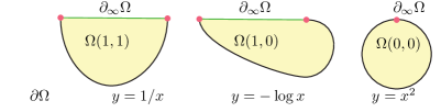
Figure 1. A projective view of some 2 dimensional $\psi$-domains

Proposition 1.5.

$\Omega(\psi)$ is a closed, unbounded, convex subset of ${\mathbb{R}}^{n}$, and a properly convex subset of $\operatorname{\mathbb{R}P}^{n}$. The horospheres $\mathcal{H}_{t}$ are smooth, strictly-convex, hypersurfaces that foliate $V_{\psi}$, and $\partial\Omega(\psi)=\mathcal{H}_{0}$.

Proof.

Since $h$ is a smooth submersion, $\mathcal{H}_{t}$ are smooth hypersurfaces that foliate $V_{\psi}$ and $\Omega=\Omega(\psi)$ is a closed submanifold of ${\mathbb{R}}^{n}$ with boundary $\mathcal{H}_{0}$. Moreover $\Omega$ is unbounded because $h_{\psi}$ is a decreasing function of $x_{s}$ where $s=\max({\bf t},1)$. The second derivative of $x^{2}$, and of $-\log(x)$, are both positive on $V_{\psi}$, so the second derivative $D^{2}h_{\psi}$ is positive semi-definite on $V_{\psi}$. For ${\bf t}<n$ it has nullity 1, given by the $x_{{\bf t}+1}$ direction. When ${\bf t}=n$ it is positive definite. The tangent space to $\mathcal{H}_{t}$ is $T_{*}\mathcal{H}_{t}=\ker Dh_{\psi}$ which does not contain the $x_{{\bf t}+1}$ direction. Thus $D^{2}h_{\psi}$ restricted to $T_{*}\mathcal{H}_{t}$ is positive definite hence $\mathcal{H}_{t}$ is strictly convex.

Suppose $\ell$ is a line segment with endpoints $a,b\in\Omega$. Set $f=h|\ell$ then $f^{\prime\prime}\geq 0$ so $f$ attains its maximum at an endpoint. Thus $f\leq\max(f(a),f(b))$ and $f(a),f(b)\leq 0$ since $a,b\in\Omega$. Thus $f\leq 0$ so $\ell\subset\Omega$ and $\Omega$ is convex.

Suppose $\ell$ is a complete affine line contained in $\Omega$. Then $\ell$ is contained in ${\mathbb{R}}_{+}^{\bf t}\times{\mathbb{R}}^{n-{\bf t}}$, so $x_{i}$ is constant along $\ell$ for $i\leq{\bf t}$. Thus ${\bf t}<n$ and $h_{\psi}|\ell=C_{1}-t+C_{2}t^{2},$ where $t$ is an affine coordinate on $\ell$. But $\ell\subset\Omega$ implies this function is nowhere positive, a contradiction. Hence $\Omega$ contains no complete affine line, and is thus properly convex . ∎

Remarks 1.6.

(a) If $\forall i\ |\psi_{i}|\geq|\psi_{i+1}|$ then $h_{\psi}$ is convex iff either $\forall i\ \psi_{i}\geq 0$ or $\forall i\ \psi_{i}<0$.
(b) It follows from Lemma 1.25 and the discussion in Section 3 of [16] that the $\mathcal{H}_{t}$ are horospheres in the sense of Busemann, and from (1.15) that they are also algebraic horospheres as defined in [16].

Definition 1.7.

The $\psi$ cusp Lie group is the subgroup, $G=G(\psi)\subset\operatorname{PGL}(n+1,{\mathbb{R}})$ that preserves each horosphere. A $\psi$-cusp is $C=\Omega(\psi)/\Gamma$ where $\Gamma\subset G$ is a torsion-free lattice.

The condition that $G(\psi)$ preserves each horosphere is equivalent to preserving the horofunction, thus $G(\psi)\subset\operatorname{PGL}(\Omega(\psi))$. It follows from Propostion 1.5 that a $\psi$-cusp is a properly-convex manifold. The torsion free hypothesis on $\Gamma$ is strictly a matter of convenience. If $\Gamma$ is a lattice in $G(\psi)$ that contains torsion then $C$ is an orbifold.

1.1. The Radial Flow

The unipotent rank is ${\bf u}=\max(n-1-{\bf t},0)$ and the rank ${\bf r}$ is defined by ${\bf r}+{\bf u}=n-1$. Then ${\bf r}=\min({\bf t},n-1)$. A more conceptual interpretation of ${\bf r}$ and ${\bf u}$ is given by Equation (1.42). It is convenient to use coordinates on $V_{\psi}$ given by

(1.8) $$(x,z,y)\in V_{\psi}=\left\{\begin{array}[]{lcl}{\mathbb{R}}_{+}^{{\bf r}}\times{\mathbb{R}}\times{\mathbb{R}}^{{\bf u}}&\textrm{if}&{\bf t}<n\\ {\mathbb{R}}_{+}^{{\bf r}}\times{\mathbb{R}}_{+}\times{\mathbb{R}}^{{\bf u}}&\textrm{if}&{\bf t}=n\end{array}\right.$$

When ${\bf t}=0$ the $x$-coordinate is empty; and when ${\bf t}\geq n-1$ then ${\bf u}=0$ so the $y$-coordinate is empty. The $z$-coordinate is called the vertical direction. This terminology is motivated by regarding the horospheres as graphs of functions, see Equation (1.19). The $y$-coordinate is called the parabolic direction and the $x$-coordinate is called the hyperbolic direction, see Equation (1.33).

Definition 1.9.

The basepoint of $\Omega(\psi)$ is $b=b_{\psi}=e_{1}+\cdots+e_{\bf t}\in{\mathbb{R}}^{n}$.

Thus for ${\bf t}=0$ the basepoint is $b=0\in{\mathbb{R}}^{n}$. The basepoint satisfies $h_{\psi}(b)=0$ so $b\in\partial\Omega$. When ${\bf t}<n$ then $b=(x_{0},z_{0},y_{0})$ where $x_{0}=(1,\cdots,1)\in{\mathbb{R}}_{+}^{{\bf r}}$ and the remaining coordinates are $0$. When ${\bf t}=n$ then $b=(1,\cdots,1)$. In projective coordinates the basepoint is $[b_{\psi}+e_{n+1}]\in\operatorname{\mathbb{R}P}^{n}$. Define

$$U=U_{\psi}={\mathbb{R}}_{+}^{{\bf r}}\times{\mathbb{R}}^{{\bf u}}$$

Radial projection is the map $\pi=\pi_{\psi}:V_{\psi}\to U_{\psi}$ given by

(1.10) $$\pi(x,z,y)=\left\{\begin{array}[]{lcl}(x,y)&\textrm{if}&{\bf t}<n\\ (x/z,y/z)&\textrm{if}&{\bf t}=n\end{array}\right.$$

Definition 1.11.

The radial flow $\Phi=\Phi^{\psi}\subset\operatorname{PGL}(n+1,{\mathbb{R}})$ is the $1$-parameter subgroup that acts on $V(\psi)$ by

(1.12) $$\Phi_{t}(x,z,y)=\Phi((x,z,y),t)=\left\{\begin{array}[]{lcl}(x,z-t,y)&\textrm{if}&{\bf t}<n\\ e^{-t}(x,z,y)&\textrm{if}&{\bf t}=n\end{array}\right.$$

In the first case the radial flow is called parabolic and in the second case it is hyperbolic. This terminology agrees with that of [17]. The orbit of a point is called a flowline. Each flowline maps to one point under radial projection. When ${\bf t}<n$ flowlines are vertical lines, and when ${\bf t}=n$ they are open rays that limit on $0\in{\mathbb{R}}^{n}$.

The reason for the name radial flow is that this group acts on $\operatorname{\mathbb{R}P}^{n}$ and there is a point $\alpha\in\operatorname{\mathbb{R}P}^{n}$ called the center of the radial flow with the property that, if a point $\beta\in\operatorname{\mathbb{R}P}^{n}$ is not fixed by the flow, then the orbit of $\beta$ is contained in the projective line containing $\alpha$ and $\beta$. Moreover $\Phi_{t}(\beta)\to\alpha$ as $t\to\infty$. The center is

(1.13) $$\alpha=[e_{{\bf t}+1}]$$

If ${\bf t}<n$ then $\alpha\in\operatorname{\mathbb{R}P}_{\infty}^{n-1}$ corresponds to the $z$-axis, and $\alpha=0\in{\mathbb{R}}^{n}$ when ${\bf t}=n$.

Observe that the radial flow has the following equivariance property:

(1.14) $$h_{\psi}(\Phi_{t}(x))=h_{\psi}(x)+t$$

This equation would need to be modified without the first factor in the definition of $h_{\psi}$ (see (1.4)) when ${\bf t}=n$. It follows that the radial flow permutes the level sets of the horofunction and hence permutes the horospheres and

(1.15) $${\mathcal{H}}_{t}=\Phi_{-t}(\partial\Omega)$$

Definition 1.16.

A product structure on a manifold $M$ is a pair of transverse foliations on $M$ determined by a diffeomorphism $P\times Q\to M$. There is a diffeomorphism $f:\partial\Omega(\psi)\times[0,\infty)\to\Omega(\psi)$ given by $f(x,t)=\Phi_{-t}(x)$. This defines a product structure on $\Omega(\psi)$, with a foliation by horospheres, and a transverse foliation by (half-)flowlines.

If $C=\Omega(\psi)/\Gamma$ is a $\psi$-cusp, then $\Gamma$ preserves this product structure, so it covers a product structure on $C$. The image in $C$ of a horosphere is called a horomanifold. The set $\Omega$ is backwards invariant which means that $\Phi_{t}(\Omega)\subset\Omega$ for all $t\leq 0$ and $\Omega$ is the backwards orbit of $\partial\Omega$

$$\Omega=\bigcup_{t\leq 0}\Phi_{t}(\partial\Omega)$$

For ${\bf t}<n$ it is convenient to introduce $\psi^{\bf t}:{\mathbb{R}}^{\bf t}\rightarrow{\mathbb{R}}$ given by

(1.17) $$\psi^{\bf t}(x)=\psi(x,0,\cdots,0)$$

Define $\operatorname{\ell og}:{\mathbb{R}}\to{\mathbb{R}}$ by

(1.18) $$\operatorname{\ell og}(x)=\left\{\begin{array}[]{lcr}0&\textrm{if}&x\leq 0\\ \log(x)&\textrm{if}&x>0\end{array}\right.$$

and extend this to a map $\operatorname{\ell og}:{\mathbb{R}}^{r}\to{\mathbb{R}}^{r}$ by applying $\operatorname{\ell og}$ componentwise. Then define $f=f_{\psi}:U\to{\mathbb{R}}$ by

(1.19) $$\begin{array}[]{rcl}f_{\psi}(x,y)&=&\left\{\begin{array}[]{lcl}-\psi^{\bf t}\circ\operatorname{\ell og}(x)+\|y\|^{2}/2&\textrm{if}&{\bf t}<n\\ \prod_{i=1}^{n-1}x_{i}^{-\psi_{i}/\psi_{n}}&\textrm{if}&{\bf t}=n\end{array}\right.\end{array}$$

The map $F=F_{\psi}:U\to\partial\Omega$ given by

(1.20) $$F(x,y)=(x,f(x,y),y)$$

is the inverse of the restriction of vertical projection $\pi|:\partial\Omega\to U$, so $\partial\Omega$ is the graph $z=f(x,y)$ of $f$ and $\Omega=\{(x,z,y):z\geq f(x,y)\}$ is the supergraph of $f$. From Definition 1.3 when ${\bf t}<n$ the horofunction is expressed more compactly as

(1.21) $$h_{\psi}(x,z,y)=-z+f_{\psi}(x,y)$$

but for ${\bf t}=n$ this does not work.

1.2. The Ideal Boundary $\partial_{\infty}\Omega$

In what follows $\psi$ is omitted from the notation. We describe the closure $\overline{\Omega}$ in $\operatorname{\mathbb{R}P}^{n}$. Identify affine space ${\mathbb{R}}^{n}$ with an affine patch in projective space $\operatorname{\mathbb{R}P}^{n}$ by identifying $(x,z,y)$ in ${\mathbb{R}}^{n}$ with $[x:z:y:1]$ in $\operatorname{\mathbb{R}P}^{n}$. Then

(1.22) $$\Omega=\{[x:z:y:1]\ |\ z\geq f(x,y),\ \ x\in{\mathbb{R}}_{+}^{{\bf r}}\}\subset\operatorname{\mathbb{R}P}^{n}$$

Observe that $\overline{\Omega}\cap{\mathbb{R}}^{n}=\Omega$. The points at infinity are $\operatorname{\mathbb{R}P}^{n-1}_{\infty}=\operatorname{\mathbb{R}P}^{n}\setminus{\mathbb{R}}^{n}$ and

(1.23) $$\overline{\Omega}=\Omega\sqcup\partial_{\infty}\Omega\qquad{\rm with}\quad\partial_{\infty}\Omega:=\overline{\Omega}\setminus\Omega\subset\operatorname{\mathbb{R}P}^{n-1}_{\infty}$$

The set $\partial_{\infty}\Omega$ is called the ideal boundary or the boundary at infinity of $\Omega$. See [19] Definition 1.17. The non-ideal boundary or just boundary of $\Omega$ is $\partial\Omega={\mathbb{R}}^{n}\cap\partial\overline{\Omega}$. Thus

$$\partial\overline{\Omega}=\partial\Omega\sqcup\partial_{\infty}\Omega.$$

Lemma 1.24.

$\partial_{\infty}\Omega(\psi)$ is the simplex of dimension ${\bf r}$

$$\partial_{\infty}\Omega(\psi)=\Delta^{{\bf r}}:=\{[x_{1}:\cdots:x_{{\bf r}+1}:{0}:\cdots:0]\ |\ x_{i}\geq 0\}$$

Proof.

From Equation (1.22) $\partial_{\infty}\Omega$ consists of all the points that are the limit of a sequence of points $[x:z:y:1]$ with $\|(x,z,y)\|\to\infty$ for which $z\geq f(x,y)$.

First assume ${\bf t}<n$, and so ${\bf t}={\bf r}$. We claim that $y/\|(x,z,y)\|\to 0$ along the sequence. If eventually $\psi^{{\bf t}}\operatorname{\ell og}(x)<\|y\|^{2}/4$ then by Equation (1.19) it follows that $z>\|y\|^{2}/4$ and, since $y/\|y\|^{2}\to 0$ as $\|y\|\to\infty$, it follows that $y/z\to 0$. Otherwise we may take a subsequence so $\psi^{{\bf t}}\operatorname{\ell og}(x)\geq\|y\|^{2}/4\to+\infty$. Since $\psi_{j}>0$ for all $j\leq{\bf r}$, this means for some $i\leq{\bf r}$ the coordinate $x_{i}$ of $x$ is positive and larger than some fixed multiple of $\exp\|y\|$, hence $y/x_{i}\to 0$. This proves the claim. Hence $\partial_{\infty}\Omega\subset\Delta^{{\bf r}}$.

From (1.19) we see that $f(e^{t}x,0)<0$ for large $t$. Then by Equation (1.22)

$$\partial_{\infty}\Omega\supset\{\lim_{t\to\infty}[e^{t}x:e^{t}z:0:1]\ |\ z\geq 0,\ \ x\in{\mathbb{R}}_{+}^{r}\}=\Delta^{{\bf r}}$$

which proves the result for ${\bf t}<n$.

When ${\bf t}=n$ then ${\bf r}=n-1$ and $\partial_{\infty}\Omega\subset\partial_{\infty}V_{\psi}=\Delta^{n-1}$. On the other hand if $v\in\operatorname{int}\Delta^{n-1}$ then $v=\lim_{t\to\infty}[tx:tz:1]$, where $x\in{\mathbb{R}}_{+}^{n-1}$ and $z\in{\mathbb{R}}_{+}$. From the definition of $f(x)$ (see Equation (1.19)), it is easy to check, when $t$ is large, that $tz>f(tx)$, hence $(tx,tz)\in\Omega$, and so $\operatorname{int}\Delta^{n-1}\subset\partial_{\infty}\Omega$. Since $\partial_{\infty}\Omega$ is closed it follows that $\Delta^{n-1}=\partial_{\infty}\Omega$. ∎

Lemma 1.25.

Every point in the relative interior of $\partial_{\infty}\Omega$ is a $C^{1}$-point, and

• $\operatorname{\mathbb{R}P}^{n-1}_{\infty}$ is the unique hyperplane in $\operatorname{\mathbb{R}P}^{n}$ that contains $\partial_{\infty}\Omega$ and is disjoint from $\Omega$.

• ${\mathbb{A}}(\Omega):=\operatorname{\mathbb{R}P}^{n}\setminus\operatorname{\mathbb{R}P}^{n-1}_{\infty}$ is the unique affine patch that contains $\Omega$ as a closed subset.

• $\operatorname{PGL}(\Omega)\subset\operatorname{Aff}({\mathbb{R}}^{n})$.

Proof.

Clearly (a) implies (b) and (c). For (a) the result follows from the following picture that we will establish. Near a point $q\in\operatorname{int}(\partial_{\infty}\Omega)$ the frontier ${\operatorname{Fr\,}}\Omega$ looks like a (flat) open set in $\Delta^{{\bf r}}$ product a hypersurface in ${\mathbb{R}}^{n-{\bf r}}$ that is $C^{1}$ close to an ellipsoid, and is thus $C^{1}$.

Now (a) is clear for ${\bf r}=n-1$. It is also clear in the case ${\bf t}=0$ since $\operatorname{cl}\Omega$ is a round ball, and $q=\partial_{\infty}\Omega$ is a single $C^{1}$ point. Thus we may suppose that ${\bf u}\geq 1$ and ${\bf r}={\bf t}>0$. We use coordinates $(a,y,w)\in{\mathbb{R}}^{{\bf r}+1}\oplus{\mathbb{R}}^{{\bf u}}\oplus{\mathbb{R}}\equiv{\mathbb{R}}^{n+1}$ where $a=(x,z)\in{\mathbb{R}}^{{\bf r}}\oplus{\mathbb{R}}$ in the coordinates above. Thus the affine patch used above is $[a:y:1]$, and $\operatorname{\mathbb{R}P}^{n-1}_{\infty}$ is $[a:y:0]$. Given $q\in\operatorname{int}(\partial_{\infty}\Omega)$ then $q=[a:0:0]$ with $a=(a_{1},\cdots,a_{{\bf r}+1})\in{\mathbb{R}}_{+}^{{\bf r}+1}$ by Lemma 1.24. Let

$$P={\mathbb{P}}({\mathbb{R}}\cdot a\oplus{\mathbb{R}}^{{\bf u}}\oplus{\mathbb{R}})\subset\operatorname{\mathbb{R}P}^{n}$$

Then $P\cong\operatorname{\mathbb{R}P}^{{\bf u}+1}$ and $P\cap\partial_{\infty}\Omega=q$. Moreover $W:=P\cap\partial\Omega\subset{\mathbb{R}}^{n}$ is the subset of $\partial\Omega$ where the $(x,z)$-coordinate is $z\cdot a$ for some $z$. We may scale $a$ so that $a_{{\bf r}+1}=1$ then $z\cdot a=(za_{1},\cdots,za_{{\bf r}},z)$. By Equation (1.3) $\partial\Omega\cap\left({\mathbb{R}}\cdot a\oplus{\mathbb{R}}^{{\bf u}}\right)$ is given by

(1.26) $${0}=h(za_{1},\cdots,za_{{\bf r}},z,y)=-z-\sum_{i=1}^{{\bf r}}\psi_{i}\log(za_{i})+\|y\|^{2}/2$$

This may be rewritten as

(1.27) $$z+\alpha\log z+\beta=\|y\|^{2}/2\qquad\alpha=\sum\psi_{i},\quad\beta=\sum\psi_{i}\log a_{i}$$

Near $q$ then $z$ is large and $W$ is $C^{0}$-close to the ellipsoid $z=\|y\|^{2}/2$ in $\operatorname{\mathbb{R}P}^{{\bf u}+1}$. We now show it is $C^{1}$-close by changing to a different affine patch using $[y:z:1]=[yz^{-1}:1:z^{-1}]=[u:1:v]$. Then $q$ is the point $(u,v)=(0,0)\in{\mathbb{R}}^{{\bf u}+1}$ and $u\in{\mathbb{R}}^{{\bf u}}$ and $v\in{\mathbb{R}}$ satisfy

(1.28) $$v^{-1}+\alpha\log v^{-1}+\beta=\|v^{-1}u\|^{2}/2$$

Which can be expressed as $f(v)=\|u\|^{2}/2$ where $f(v)=v-\alpha v^{2}\log v+\beta v^{2}$ for $v\neq 0$. There is a $C^{1}$ extension of $f$ given by $f(0)=0$, then $f^{\prime}(0)=1$, so by the inverse function theorem near $0\in{\mathbb{R}}^{{\bf u}}\oplus{\mathbb{R}}$ we have $v=f^{-1}(\|u\|^{2}/2)$ is $C^{1}$ close to $v=\|u\|^{2}/2$ at $q$. In particular $q$ is a $C^{1}$ point of $\operatorname{cl}W$. It is interesting that $f^{\prime\prime}(v)\to\infty$ as $v\to 0$.

Let $H\cong\operatorname{\mathbb{R}P}^{n-1}$ be a supporting hyperplane to ${\operatorname{Fr\,}}\Omega$ at $q$, then since $q$ is a $C^{1}$ point of $\operatorname{cl}(W)$ in $P$ it follows that $H$ contains $Q:=P\cap\operatorname{\mathbb{R}P}_{\infty}^{n-1}$. Furthermore, $\dim Q=\dim P-1={\bf u}$. Since $q\in\operatorname{int}(\partial_{\infty}\Omega)$ and $H$ is a supporting hyperplane, it follows that $H$ contains $\partial_{\infty}\Omega$. By Lemma 1.24, $\dim\partial_{\infty}\Omega={\bf r}$ and hence $\dim(\partial_{\infty}\Omega)+\dim Q={\bf r}+{\bf u}=n-1=\dim H.$ Since $\partial_{\infty}\Omega$ and $Q$ are transverse in $H$ it follows that $H$ is the unique hyperplane that contains $\partial_{\infty}\Omega\cup Q$. ∎

The next result implies that a generalized cusp has a natural affine structure that is a stiffening of the projective structure.

Proposition 1.29.

Let $\Omega=\Omega(\psi),\ \Phi=\Phi^{\psi},\ h=h_{\psi}$ and let $\color[rgb]{0,0,0}\alpha$ be the center of $\Phi$. Let $\Omega^{\prime},\Phi^{\prime},h^{\prime}$ and ${\color[rgb]{0,0,0}\alpha}^{\prime}$ be the corresponding objects for $\psi^{\prime}$. Suppose that $P\in\operatorname{PGL}(n+1,{\mathbb{R}})$ and $P(\Omega)=\Omega^{\prime}$ then

• ${\bf t}={\bf t}^{\prime}$

• $P({\color[rgb]{0,0,0}\alpha})={\color[rgb]{0,0,0}\alpha}^{\prime}$

• $P\in\operatorname{Aff}({\mathbb{R}}^{n})$

• $\Phi^{\prime}=P\cdot\Phi\cdot P^{-1}$

• $\exists\ {\color[rgb]{0,0,0}c}>0\ \ \forall\ t\ \ \ \Phi^{\prime}_{{\color[rgb]{0,0,0}c}t}=P\cdot\Phi_{t}\cdot P^{-1}$

• $h^{\prime}\circ P={\color[rgb]{0,0,0}c}\cdot h$

• $P$ sends the product structure of $\Omega$ to that of $\Omega^{\prime}$

Proof.

Clearly $P(\partial_{\infty}\Omega)=\partial_{\infty}\Omega^{\prime}$. By Lemma 1.24 $\partial_{\infty}\Omega$ is a simplex of dimension ${\bf r}=\min({\bf t},n-1)$ and it follows that if ${\bf t}\leq n-2$ then ${\bf t}={\bf t}^{\prime}$. It remains to distinguish ${\bf t}=n-1$ from ${\bf t}=n$ in a projectively invariant way.

Claim If ${\bf t}\geq n-1$ then there is a unique minimal closed $n$-simplex $\Delta\subset\operatorname{\mathbb{R}P}^{n}$, such that $\Omega\subset\Delta$ and $\partial_{\infty}\Omega$ is a face of $\Delta$, if and only if ${\bf t}=n$.

In the case ${\bf t}=n$ then $\Delta$ is the closure in $\operatorname{\mathbb{R}P}^{n}$ of ${\mathbb{R}}_{+}^{n}\subset{\mathbb{R}}^{n}$. Minimality and uniqueness follows from the fact that $\partial\Omega$ is asymptotic in ${\mathbb{R}}_{+}^{n}$ to $\partial\Delta$ near $\operatorname{\mathbb{R}P}^{n-1}_{\infty}$. Consider a ray $\gamma:[0,\infty)\to{\mathbb{R}}_{+}^{n}$ then $h(\gamma(t))\to-\infty$ as $t\to\infty$. Thus $\gamma(t)\in\Omega$ for $t$ large. If $\Delta^{\prime}\neq\Delta$, and $\Delta^{\prime}$ contains $\Omega$, and $\Delta^{\prime}=p*\partial_{\infty}\Omega$, then there is such a ray in $\partial\Delta^{\prime}$, unless $\Delta^{\prime}\supset\Delta$. Thus any simplex that contains $\Omega$ also contains $\Delta$.

In the case ${\bf t}=n-1$ the analysis below shows that there is a projective plane $H\cong\operatorname{\mathbb{R}P}^{2}$ such that $\Omega\cap H$ looks like $\Omega(1,0)$ in Figure $1$. This implies no such $\Delta$ exists, which proves the claim and (a).

By Equation (1.13), ${\color[rgb]{0,0,0}\alpha}=[e_{{\bf t}+1}]$. When ${\bf t}=n$ then ${\bf t}^{\prime}=n$ and uniqueness of $\Delta$ implies $P(\Delta)=\Delta^{\prime}$. Observe that ${\color[rgb]{0,0,0}c}=[e_{n+1}]$ is the unique vertex of $\Delta$ that is not in $\partial_{\infty}\Omega$. Thus $P({\color[rgb]{0,0,0}\alpha})={\color[rgb]{0,0,0}\alpha}^{\prime}$ in this case. When ${\bf t}=0$ then ${\color[rgb]{0,0,0}\alpha}=[e_{1}]=\partial_{\infty}\Omega$ and ${\color[rgb]{0,0,0}\alpha}^{\prime}=\partial_{\infty}\Omega^{\prime}$ so (b) follows in this case.

For (b) this leaves the case $0<{\bf t}<n$ then ${\color[rgb]{0,0,0}\alpha}=[e_{{\bf t}+1}]\in\operatorname{\mathbb{R}P}^{n-1}_{\infty}$. By Lemma 1.24 the vertices of $\partial_{\infty}\Omega$ are $[e_{s}]$ with $1\leq s\leq{\bf t}+1$. Given $s\leq{\bf t}$ let $H\cong\operatorname{\mathbb{R}P}^{2}$ be any projective plane that contains the vertices $[e_{{\bf t}+1}]$ and $[e_{s}]$ of $\Delta^{\bf r}$, and also some point $[(v_{1},\cdots,v_{n},1)]\in\partial\Omega$. The intersection of $H$ with the affine patch ${\mathbb{R}}^{n}$ is the affine subspace $V=\langle e_{s},e_{{\bf t}+1}\rangle+(v_{1},\cdots,v_{n})$. Using Definition 1.3, the restriction of $h=h_{\psi}$ to $V$ is

$$f(X,Y):=h(Xe_{s}+Ye_{{\bf t}+1}+v)=-Y-\psi_{s}\log(X+v_{s})+C$$

where $C$ is a constant independent of $X$ and $Y$ that depends on $v$. The curve $V\cap\partial\Omega$ is given by $f(X,Y)=0$. The affine change of coordinates $(X,Y)=(x-v_{s},\psi_{s}y+C)$ maps this curve to $y=-\log x$. It follows that, on the curve $H\cap\partial\overline{\Omega}$, the point $[e_{s}]$ is $C^{1}$ and $[e_{{\bf t}+1}]$ is not $C^{1}$ (see the middle domain in Figure 1). Thus the center ${\color[rgb]{0,0,0}\alpha}=[e_{{\bf t}+1}]$ is a vertex of $\partial_{\infty}\Omega$ that is distinguished (in a projectively invariant way) from every other vertex $[e_{s}]$ of $\partial_{\infty}\Omega$. This completes the proof of (b).

By Lemma 1.25(c) $P$ preserves $\operatorname{\mathbb{R}P}^{n-1}_{\infty}$ proving (c). The radial flow is characterized as the one-parameter subgroup $\Phi\subset\operatorname{PGL}$ that fixes every point in the stationary hyperplane, preserves every line containing the center, and no non-trivial element fixes any other point. This and (b) implies (d). Every automorphism of ${\mathbb{R}}$ is multiplication by some ${\color[rgb]{0,0,0}c}\neq 0$. Since $\Omega$ is backward invariant, ${\color[rgb]{0,0,0}c}>0$ which proves (e). By Equation (1.14) $h^{\prime}\circ P={\color[rgb]{0,0,0}c}\cdot h$ which proves (f). The level sets of $h$ gives the foliation by horospheres, so $P$ preserves this foliation. Similarly $P$ preserves the $\Phi$-orbits of points, which are the flowlines, giving (g). ∎

1.3. The Structure of $G(\psi)$

Theorem 1.45 gives a decomposition of the group $G(\psi)\cong T(\psi)\rtimes O(\psi)$ corresponding to the decomposition $\operatorname{Isom}({\mathbb{R}}^{n})\cong{\mathbb{R}}^{n}\rtimes O(n)$ into translation and orthogonal subgroups. We begin by describing the translation subgroup $T(\psi)$.

Recall the standard identification of the affine group $\operatorname{Aff}({\mathbb{R}}^{n})$ with the subgroup

$$\left\{\begin{pmatrix}A&v\\ 0&1\end{pmatrix}\ :\ A\in\operatorname{GL}(n,{\mathbb{R}}),\ v\in{\mathbb{R}}^{n}\right\}\subset\operatorname{GL}(n+1,{\mathbb{R}})$$

The affine action on ${\mathbb{R}}^{n}$ is realized by the embedding ${\mathbb{R}}^{n}\to{\mathbb{R}}^{n+1}$ given by $a\mapsto(a,1)$.

Our next task is to define a subgroup of $G(\psi)$, called the translation subgroup $T(\psi)\cong{\mathbb{R}}^{n-1}$, that acts simply transitively on $\partial\Omega(\psi)$. We first define the enlarged translation group $T_{{\bf t}}\cong{\mathbb{R}}^{n}$ that acts simply transitively on $V_{\psi}={\mathbb{R}}_{+}^{\bf t}\times{\mathbb{R}}^{n-{\bf t}}$. Then $T(\psi)=\ker\psi_{*}$ for a certain homomorphism $\psi_{*}:T_{{\bf t}}\to{\mathbb{R}}$ derived from $\psi$. The enlarged translation group is the direct sum of the translation group and the radial flow: $T_{{\bf t}}=T(\psi)\oplus\Phi^{\psi}$.

The enlarged translation group $T_{{\bf t}}$ has Lie algebra $\mathfrak{t}_{{\bf t}}$ that is the image of the map $\Psi_{{\bf t}}:{\mathbb{R}}^{n}\to\mathfrak{gl}(n+1,{\mathbb{R}})$ given by

(1.30) $$\Psi_{{\bf t}}(X,Z,Y):=\begin{pmatrix}\operatorname{Diag}(X)&0\\ 0&\begin{pmatrix}0&Y^{t}&Z\\ 0&0&Y\\ 0&0&0\end{pmatrix}\end{pmatrix}$$

Here $X\in{\mathbb{R}}^{\bf r}$ and $Z\in{\mathbb{R}}$ and $Y\in{\mathbb{R}}^{{\bf u}}$, except when ${\bf u}=0$ there is no $Y$, and when ${\bf t}=n$ there is no $Z$ and the bottom right block is $(0)$. It is easy to check that all Lie brackets in $\mathfrak{t}_{{\bf t}}$ are $0$ and so $\mathfrak{t}_{{\bf t}}$ is an abelian Lie subalgebra, and $T_{{\bf t}}\cong{\mathbb{R}}^{n}$ as a Lie group. Define $m_{{\bf t}}(X,Z,Y)=\exp\Psi_{{\bf t}}(X,Z,Y)$ then $T_{{\bf t}}$ consists of all matrices

(1.31) $$m_{{\bf t}}(X,Z,Y)=\begin{pmatrix}\exp\operatorname{Diag}(X)&0\\ 0&\begin{pmatrix}1&Y^{t}&Z+\|Y\|^{2}/2\\ 0&I_{{\bf u}}&Y\\ 0&0&1\end{pmatrix}\end{pmatrix}$$

Definition 1.32.

The translation group $T:=T(\psi)$ is the kernel of the homomorphism $\psi_{*}:T_{{\bf t}}\to{\mathbb{R}}$ defined for ${\bf t}<n$ by $\psi_{*}(m_{{\bf t}}(X,Z,Y))=\psi^{\bf t}(X)+Z$, and for ${\bf t}=n$ by $\psi_{*}(m_{n}(X))=(\sum\psi_{i})^{-1}\psi(X)$.

For ${\bf t}<n$, the translation group $T(\psi)$ consists of the matrices $m_{{\bf t}}(X,Y,Z)$ given by Equation (1.31) for which $Z=-\psi^{\bf t}(X)$. It will occasionally be convenient to write the translation group as the image of a linear map, instead of as the kernel of a linear map. For ${\bf t}<n$ the translation group $T(\psi)$ is the image of $m^{*}_{\psi}:{\mathbb{R}}^{\bf r}\times{\mathbb{R}}^{{\bf u}}\to\operatorname{GL}(n+1,{\mathbb{R}})$ given by

(1.33) $$m^{*}_{\psi}(X,Y)=\begin{pmatrix}\exp\operatorname{Diag}(X)&0\\ 0&\begin{pmatrix}1&Y^{t}&\|Y\|^{2}/2-\psi^{\bf t}(X)\\ 0&I_{{\bf u}}&Y\\ 0&0&1\end{pmatrix}\end{pmatrix}$$

and for ${\bf t}=n$ the translation group $T(\psi)$ is the image of $m^{*}_{\psi}:\ker\psi\to\operatorname{GL}(n+1,{\mathbb{R}})$ by

(1.34) $$m^{*}_{\psi}(X)=\begin{pmatrix}\exp\operatorname{Diag}(X)&0\\ 0&1\end{pmatrix}$$

It is worth pointing out that with this formalism the case ${\bf t}=n-1$ means ${\bf u}=0$ and gives

(1.35) $$m^{*}_{\psi}(X,Y)=\begin{pmatrix}\exp\operatorname{Diag}(X)&0\\ 0&\begin{pmatrix}1&-\psi^{\bf t}(X)\\ 0&1\end{pmatrix}\end{pmatrix}$$

Lemma 1.36.

$T_{{\bf t}}$ acts simply transitively on $V_{\psi}={\mathbb{R}}_{+}^{\bf t}\times{\mathbb{R}}^{n-{\bf t}}$ and

1. $h_{\psi}\circ m_{\bf t}{(X,Z,Y)}=h_{\psi}-\psi_{\ast}\circ m_{\bf t}{(X,Z,Y)}$

2. $T(\psi)$ is the the subgroup of $T_{{\bf t}}$ that preserves $h_{\psi}$

3. $T(\psi)$ preserves the foliation of $V_{\psi}$ by horospheres

4. $T(\psi)$ preserves the transverse foliation by flowlines.

Proof.

It is clear the action is simply transitive, and that (a) implies both (b) and (c), and that (d) holds. We first prove (a) in the case ${\bf t}<n$. From Equation (1.21)

$$-h_{\psi}(x,z,y)=z+\psi^{\bf t}(\operatorname{\ell og}x)-\|y\|^{2}/2$$

and

$$\begin{array}[]{l}m_{{\bf t}}(X,Z,Y)(x,z,y)^{t}\\ =(\exp(X_{1})x_{1},\cdots,\exp(X_{\bf r})x_{\bf r},z+Y\cdot y+Z+\|Y\|^{2}/2,Y_{1}+y_{1},\cdots,Y_{{\bf u}}+y_{{\bf u}})^{t}\end{array}$$

so

$$\begin{array}[]{l}-h_{\psi}(m_{{\bf t}}(X,Z,Y)(x,z,y)^{t})\\ =z+Y\cdot y+Z+\|Y\|^{2}/2+\psi^{\bf t}\operatorname{\ell og}(\exp(X_{1})x_{1},\cdots,\exp(X_{\bf r})x_{\bf r})-\|Y+y\|^{2}/2\\ =z+Z+\psi^{\bf t}(X+\operatorname{\ell og}x)-\|y\|^{2}/2\\ =(Z+\psi^{\bf t}(X))+\left(z+\psi^{\bf t}(\operatorname{\ell og}x)-\|y\|^{2}/2\right)\\ =\psi_{*}(m{{}_{\bf t}}(X,Z,Y))-h_{\psi}(x,z,y)\\ \end{array}$$

A similar but simpler argument applies when ${\bf t}=n$, by omitting the $Y$ and $Z$ coordinates. ∎

Lemma 1.37.

$T(\psi)\subset G(\psi)$ and $T(\psi)$ acts simply transitively on $\partial\Omega(\psi)$.

Proof.

By Equations (1.33) and (1.31) $T(\psi)$ is the subgroup of $T_{{\bf t}}$ given by $Z=-\psi^{\bf t}(X)$. It follows from (Lemma 1.36)(b) that $T(\psi)$ is the subgroup of $T_{{\bf t}}$ that preserves the horofunction, hence $T(\psi)\subset G(\psi)$. Simple transitivity on $\partial\Omega(\psi)$ also follows from Lemma 1.36. ∎

The following is from [16]. If $\Omega$ is open and properly convex and $A\in\operatorname{PGL}(\Omega)$ the displacement distance of $A$ is

(1.38) $$\delta(A)=\inf\{d_{\Omega}(x,Ax)|x\in\Omega\}$$

where $d_{\Omega}$ is the Hilbert metric on $\Omega$. Then $A$ is called hyperbolic if $\delta(A)>0$, and elliptic if $A$ fixes a point in $\Omega$, otherwise it is called parabolic if $A$ does not fix any point in $\Omega$ and $\delta(A)=0$. Moreover $\delta(A)=0$ if and only if all eigenvalues of $A$ have the same modulus. A parabolic $A\in\operatorname{PGL}(n+1,{\mathbb{R}})$ is called standard if it is conjugate into $PO(n,1)\cong\operatorname{Isom}({\mathbb{H}}^{n})$. This is equivalent to there are $\lambda,t\neq 0$ such that $\lambda A$ is conjugate in $\operatorname{GL}(n+1,{\mathbb{R}})$ into

(1.39) $$\begin{pmatrix}1&t&t^{2}/2\\ 0&1&t\\ 0&1&1\end{pmatrix}\oplus O(n-2)$$

Standard parabolics have a Jordan block of size $3$. It follows from Equation (1.33) that:

Lemma 1.40.

The parabolic subgroup $P(\psi)\subset T(\psi)$ consists of all unipotent elements of $T(\psi)$. Moreover $P(\psi)=\{m^{*}_{\psi}(0,Y):Y\in{\mathbb{R}}^{{\bf u}}\}$ and non-trivial elements are standard standard parabolics.

Let $T_{1}\subset T_{2}\subset T$ where $T_{1}$ is the subgroup of diagonalizable elements, and $T_{2}$ is the subgroup of elements for which every Jordan block has size at most $2$. This description is invariant under conjugacy, and

(1.41) $$\begin{array}[]{rcccl}T_{1}&=&{T_{1}(\psi)}&=&\{m^{*}_{\psi}(X,0):X\in\ker\psi^{{\bf r}}\}\\ T_{2}&=&{T_{2}(\psi)}&=&\{m^{*}_{\psi}(X,0):X\in{\mathbb{R}}^{{\bf r}}\}\end{array}$$

Then $T(\psi)=P(\psi)\oplus T_{2}$, and $\dim T_{2}=1+\dim T_{1}$ if $0<{\bf t}<n$. Non-trivial elements of $T_{2}$ are hyperbolic. A weight is a homomorphism $\lambda:T(\psi)\to{\mathbb{R}}^{\times}$ such that $\det(A-\lambda I)=0$ for all $A\in T(\psi)$. Let $\mathcal{W}$ be the set of such weights. Here are conceptual descriptions of ${\bf u}$, ${\bf r}$ and ${\bf t}$:

(1.42) $${\bf u}=\dim P(\psi)\qquad{\bf r}=\dim T_{2}(\psi)\qquad{\bf t}=|\mathcal{W}|-1$$

Thus ${\bf r}$ is the dimension of the subgroup of hyperbolics in the translation group, ${\bf u}$ the dimension of the unipotent (parabolic) subgroup, $\dim T(\psi)={\bf u}+{\bf r}=n-1$.

Definition 1.43.

$O(\psi)$ is the subgroup of $G(\psi)$ that fixes the basepoint $b_{\psi}$.

When $\psi=0$ (the case of a cusp in ${\mathbb{H}}^{n}$) then $O(\psi)\cong O(n-1)$ is the subgroup of $O(n)\subset\operatorname{Aff}({\mathbb{R}}^{n})$ that fixes $e_{1}$. At the other extreme, when ${\bf t}=n$ and all the coordinates of $\psi$ are distinct, then $O(\psi)$ is trivial. The general case is:

Proposition 1.44.

Suppose $\psi\in A$ has type ${\bf t}={\bf t}(\psi)$. Let $e_{1},\cdots,e_{n+1}$ be the standard basis of ${\mathbb{R}}^{n+1}$ and $S(\psi)\subset\operatorname{GL}({\bf t},{\mathbb{R}})$ be the subgroup that permutes $\{e_{1},\cdots,e_{\bf t}\}$ and preserves the vector $\sum_{i=1}^{\bf t}\psi_{i}e_{i}.$ Then $O(\psi)$ is equal to the subgroup $O^{\prime}(\psi)\subset\operatorname{Aff}({\mathbb{R}}^{n})\subset\operatorname{GL}(n+1,{\mathbb{R}})$ given by

$$\begin{array}[]{cccccccc}&{\bf t}<n-1&&&{\bf t}=n-1&&&{\bf t}=n\\ O^{\prime}(\psi)=&\begin{pmatrix}S(\psi)&0&0&0\\ 0&1&0&0\\ 0&0&O({\bf u})&0\\ 0&0&0&1\end{pmatrix}&&&\begin{pmatrix}S(\psi)&0&0\\ 0&1&0\\ 0&0&1\end{pmatrix}&&&\begin{pmatrix}S(\psi)&0\\ 0&1\end{pmatrix}\end{array}$$

Proof.

It is easy to check that $O^{\prime}(\psi)$ fixes the basepoint and preserves the horofunction $h=h_{\psi}$ so $O^{\prime}(\psi)\subset O(\psi)$. For the converse, $\operatorname{PGL}(\Omega)\subset\operatorname{Aff}({\mathbb{R}}^{n})$ so $O(\psi)\subset\operatorname{Aff}({\mathbb{R}}^{n})$. It is easy to check the result when ${\bf t}=n$, so assume ${\bf t}<n$. From Equation (1.4) the horofunction $h:{\mathbb{R}}_{+}^{\bf t}\times{\mathbb{R}}^{n-{\bf t}}\to{\mathbb{R}}$ is

$$h(x,z,y)=-\psi^{\bf t}(\operatorname{\ell og}(x)){-}z{+}\|y\|^{2}/2$$

If $\tau\in O(\psi)$ then $h=h\circ\tau$. Given a unit vector $u=(x,z,y)\in{\mathbb{R}}^{\bf r}\times{\mathbb{R}}\times{\mathbb{R}}^{{\bf u}}$ there is an affine line $\ell_{u}$ in ${\mathbb{R}}^{n}$ containing the basepoint that is the image of the map $\gamma_{u}(t)=b+t\cdot u$. The horofunction is only defined on the subset of this line in $V_{\psi}$. This gives a function $f=f_{u}:I_{u}\to{\mathbb{R}}$ defined on some maximal interval $I_{u}\subset{\mathbb{R}}$ by

$$f_{u}(t):=h\circ\gamma_{u}(t)={-}tz{+}t^{2}\|y\|^{2}/2-\sum_{i=1}^{{\bf t}}\psi_{i}\log(1+tx_{i})$$

here $x=(x_{1},\cdots,x_{{\bf t}})$. We distinguish two classes of line $\ell_{u}$ according to the behaviour of $f$. The function $f$ is defined on $I_{u}={\mathbb{R}}$ iff $x=0$, and it is defined on $[0,\infty)\subset I_{u}$ and grows logarithmically as $t\to\infty$ iff $z=y=0$ and each coordinate of $x$ is non-negative. Since $\tau$ is affine, it preserves the smallest affine subspace that contains all the lines of a given type. Since $\tau$ fixes the basepoint $b$, and preserves the type of lines, $\tau$ preserves the affine subspaces $P=b+\langle e_{1},\cdots,e_{\bf t}\rangle$ and $Q=b+\langle e_{{\bf t}+1},\cdots,e_{n}\rangle$. Notice that $P=\langle e_{1},\cdots,e_{\bf t}\rangle$.

By Lemmas 1.24 and 1.29, $\tau$ preserves the simplex spanned by the ideal boundary $\partial_{\infty}\Omega$ and the center $\alpha$ of the radial flow $\Phi$ of $\Omega$ (this simplex is exactly $\partial_{\infty}\Omega$ unless ${\bf t}=n$ in which case it is larger). It follows that $\tau$ permutes the vertices $\{[e_{i}]:1\leq i\leq{\bf t}+1\}$ of this simplex. On $P$ we have $h(x_{1}e_{1}+\cdots x_{\bf t}e_{\bf t})=-\sum\psi_{i}\log x_{i}$. Since $\tau|P$ preserves $h$, it follows that must $\tau$ preserve $\psi|P$. Thus the first ${\bf t}$ columns of $\tau$ are as shown in $O^{\prime}(\psi)$.

The only $u$ for which $f_{u}$ is linear is when $u=\pm e_{{\bf t}+1}$. Since $\tau$ fixes the basepoint and preserves $h$ it follows that $\tau$ maps the line $\ell_{e_{{\bf t}+1}}$ to itself by the identity. This gives column $({\bf t}+1)$ in $O^{\prime}(\psi)$. Finally $f_{u}$ is a quadratic polynomial with a minimum of $0$ at the basepoint exactly when $x=0$ and $z=0$ so $u\in\langle e_{{\bf t}+2},\cdots,e_{n}\rangle$. On this subspace $h(y_{1}e_{{\bf t}+2}+\cdots+y_{{\bf u}}e_{n})=\|y\|^{2}/2$. Since $\tau$ preserves this function, the columns ${\bf t}+2$ to $n$ of $\tau$ in $O^{\prime}(\psi)$ (those that contain $O({\bf u})$) are as shown. Since $\tau$ is affine and fixes the basepoint the last column is as shown in $O(\psi^{\prime})$. The result now follows.∎

A morphism between two geometries $(G,X)$ and $(H,Y)$ is a homomorphism $\rho:G\to H$, and an immersion $f:X\to Y$, such that

$$\forall g\in G,x\in X\quad f(g\cdot x)=\rho(g)\cdot(fx)$$

If $f$ and $\rho$ are both inclusions we say $(G,X)$ is a subgeometry of $(H,Y)$.

Theorem 1.45.

$G(\psi)=T(\psi)\rtimes O(\psi)$ and:

• $T(\psi)\cong{\mathbb{R}}^{n-1}$ acts simply transitively on $\partial\Omega(\psi).$

• $O(\psi)$ is the stabilizer of a point in $\partial\Omega(\psi)$.

• $O(\psi)$ is a maximal compact subgroup of $G(\psi)$.

• $(G(\psi),\partial\Omega)$ is isomorphic to a subgeometry of $(\operatorname{Isom}({\mathbb{E}}^{n-1}),{\mathbb{E}}^{n-1})$

• $T(\psi)$ is the unique Lie subgroup of $G(\psi)$ isomorphic to ${\mathbb{R}}^{n-1}$.

• $T(\psi)$ is the subgroup of $G(\psi)$ of elements all of whose eigenvalues are positive.

Proof.

(a) and (b) follow from Lemma 1.37 and Definition 1.43. By Proposition 1.44 $O(\lambda)$ is compact giving part of (c). By (a) we may regard the orbit map $\tau:T(\psi)\to\partial\Omega$ given by $\tau(g)=g(b_{\psi})$ as an identification, then $O(\psi)$ acts smoothly on $T(\psi)$ fixing the identity. The derivative of this action acts linearly on the Lie algebra of $T(\psi)$ as a compact group. Thus there is an inner product on the Lie algebra of $T(\psi)$ that is preserved by this action. Using left translation gives a flat Riemannian metric on $T(\psi)$, which is therefore isometric to ${\mathbb{E}}^{n-1}$. Then $\tau$ conjugates the action of $G(\psi)$ on $\partial\Omega$ into a subgroup of $\operatorname{Isom}({\mathbb{E}}^{n-1})$. This proves (d).

Clearly (d) implies the maximality claim in (c), as well as (e), and also implies that $G(\psi)$ is an internal semidirect product as claimed. A Euclidean isometry is conjugate by a translation to the composition of an orthogonal element and a translation that commute. It follows by (d) that $g\in G(\psi)$ is conjugate to $a\cdot t$ with $t\in T(\psi)$ and $a\in O(\psi)$ and $a\cdot t=t\cdot a$. By definition all eigenvalues of elements of $T(\psi)$ are positive. Since $a$ and $t$ commute the eigenvalues of $a\cdot t$ are products of eigenvalues of $a$ and of $t$. Thus, if all the eigenvalue of $g$ are positive, then all those of $a$ are positive. An element of the orthogonal group with all eigenvalues positive is trivial which proves (f). ∎

Corollary 1.46.

Every parabolic in $G(\psi)\subset\operatorname{GL}(n+1,{\mathbb{R}})$ is conjugate into $O(n,1)$.

Proof.

An element $g\in G(\psi)$ is parabolic iff all eigenvalues of $g$ have modulus $1$ and $g$ is not conjugate into $O(n+1)$. Such $g$ is conjugate to $a\cdot t$ with $a\in O(\psi)$ and $1\neq t\in T(\psi)$ and $a\cdot t=t\cdot a$. Since the eignevalues of $t$ are all positive, they are all $1$, so $t\in P(\psi)$. Thus $g$ is a standard parabolic. ∎

From Equation (1.12) the radial flow $\Phi\subset\operatorname{GL}(n+1,{\mathbb{R}})$ is given by

(1.47) $$\begin{array}[]{ccc}&{\bf t}<n&{\bf t}=n\\ \\ \Phi_{s}=&\exp\begin{pmatrix}0_{{\bf t}\times{\bf t}}&0&0\\ 0&0&-s\\ 0&0_{n-{\bf t}\times n-{\bf t}}&0\end{pmatrix}&\ \ \ \ \exp\begin{pmatrix}-s\operatorname{I}_{n\times n}&0\\ 0&0\end{pmatrix}\end{array}$$

Observe that the one-parameter group $\Phi$ is a subgroup of $T_{{\bf t}}$ and $T_{{\bf t}}=T{(\psi)}\oplus\Phi$. In particular $T{=T(\psi)}$ commutes with the radial flow, so $T$ sends radial flows lines to radial flow lines. Thus $T$ induces an action on the space of flowlines in $V_{\psi}$, and radial projection identifies this space with $U_{\psi}$. The action of $T$ on $U_{\psi}$ is affine, and given by omitting row and column ${\bf t}+1$ to give

$$\begin{pmatrix}\exp\operatorname{Diag}(X)&0&0\\ 0&I_{{\bf u}}&Y\\ 0&0&1\end{pmatrix}\quad Y\in{\mathbb{R}}^{{\bf u}}$$

with both $Y$ and $I_{{\bf u}}$ interpreted as empty for ${\bf u}=0$. This happens when ${\bf r}=n-1$. In the case ${\bf t}<n$ then $X\in{\mathbb{R}}^{\bf r}$ and when ${\bf t}=n$ then $X\in\ker\psi^{\bf t}$. From this it follows that:

Lemma 1.48.

Under radial projection $\pi:V_{\psi}\to U_{\psi}$ the action of $T(\psi)$ on $V_{\psi}$ is semi-conjugate to a simply transitive affine action of $T(\psi)$ on $U_{\psi}$, that is topologically conjugate to the action of ${\mathbb{R}}^{n-1}$ on itself by translation.

Proof.

The second conclusion follows by conjugating with the map ${\mathbb{R}}_{+}^{{\bf r}}\times{\mathbb{R}}^{{\bf u}}\to{\mathbb{R}}^{n-1}$ given by $(x,y)\mapsto(\operatorname{\ell og}x,y)$. ∎

1.4. Domains preserved by $T(\psi)$

$\Omega=\Omega(\psi)$ is not the only properly convex domain preserved by $T=T(\psi)$. If $B\in\operatorname{Aff}({\mathbb{R}}^{n})$ normalizes $T$, then $T$ also preserves $B(\Omega)$. However the cusp $\Omega/\Gamma$ is affinely equivalent to $B(\Omega)/\Gamma$. When $T$ is diagonal there is a different class of examples given by gluing two copies of $\Omega$ along $\operatorname{int}(\partial_{\infty}\Omega)$, and then deleting one boundary component.

Definition 1.49.

$\SS({\bf t})\subset\operatorname{GL}(n+1,{\mathbb{R}})$ is the the group of all diagonal matrices $\epsilon$ with $\epsilon_{i,i}=\pm 1$ for $i\leq{\bf t}={\bf t}(\psi)$ and $\epsilon_{i,i}=1$ for $i>{\bf t}$. Moreover $\SS({\bf t},\psi)$ is the subgroup of $\SS({\bf t})$ that normalizes $G(\psi)$ .

Lemma 1.50.

$\SS({\bf t})$ centralizes $T(\psi)$; and $\SS({\bf t},\psi)$ consists of all $\epsilon\in\SS({\bf t})$ such that $\epsilon_{k,k}=\epsilon_{j,j}$ whenever $\psi_{k}=\psi_{j}$. Furthermore, $\SS({\bf t},\psi)$ also centralizes $G(\psi)$.

Proof.

The first statement easily follows from the presentation of $T(\psi)$, see Equations (1.34) and (1.33). By Proposition 1.44, we may regard $S(\psi)$ and $O({\bf u})$ as subgroups of $\operatorname{Aff}({\mathbb{R}}^{n})\subset\operatorname{GL}(n+1,{\mathbb{R}})$ acting on ${\mathbb{R}}^{n}$. It is easy to check that $\SS({\bf t})$ centralizes $O({\bf u})$. An element $A\in S(\psi)$ permutes the $x_{i}$ coordinates for $1\leq i\leq{\bf t}$, and $\epsilon\in\SS({\bf t})$ assigns a sign to each of these coordinates so that

(1.51) $$(\epsilon A\epsilon)_{j,k}=\epsilon_{j,j}\epsilon_{k,k}A_{j,k}$$

is a signed permutation. Thus $\epsilon\in\SS({\bf t},\psi)$ if and only if $\epsilon_{k,k}=\epsilon_{j,j}$ whenever $\psi_{k}=\psi_{j}$. Moreover in this case $\epsilon$ commutes with $A$. ∎

For $1\leq i\leq{\bf t}$ let $H_{i}\subset\operatorname{\mathbb{R}P}^{n}$ be the hyperplane $x_{i}=0$. Then $X:=\operatorname{\mathbb{R}P}^{n}\setminus(\operatorname{\mathbb{R}P}_{\infty}^{n-1}\cup_{i}H_{i})$ has $2^{\bf t}$ components, each affinely equivalent to $V_{\psi}$. It is easy to check that:

Lemma 1.52.

$\SS({\bf t})$ acts simply transitively on the components of $X$, and $T_{{\bf t}}\oplus\SS({\bf t})$ acts simply transitively on $X$.

It follows that the only projective hyperplanes that are preserved by $T(\psi)$ are $\operatorname{\mathbb{R}P}_{\infty}^{n-1}$ and the hyperplanes $H_{i}$. If $g\in\SS({\bf t})\oplus\Phi^{\psi}$ then $g(\Omega)$ is called a standard domain. Since $g$ normalizes $T(\psi)$, this domain is preserved by $T(\psi)$. Since $\color[rgb]{0,0,0}\Phi_{t}\left(\Omega(\psi)\right)\subset\Phi_{s}\left(\Omega(\psi)\right)$ if $t\leq s$, it follows that standard domains intersect if and only if one contains the other.

A properly convex set $U\cong\partial U\times[0,\infty)$ that is preserved by the action of $T(\psi)$ is called reducible if there is a projective hyperplane $H$ that is preserved by $T(\psi)$ and $H\cap U\neq\emptyset$, otherwise $U$ is irreducible. If such $H$ exists then $H$ separates $U$ into two properly convex sets that are preserved by $T(\psi)$. It follows from the above that, if $U$ is irreducible, then $U$ is contained in some component of $X$.

Lemma 1.53.

If $U\subset\operatorname{\mathbb{R}P}^{n}$ is an irreducible properly convex set that is preserved by $T(\psi)$, and $U\cong\partial U\times[0,\infty)$, then $U$ is a standard $\psi$-domain. Moreover there is a unique $g\in\SS({\bf t})\oplus\Phi^{\psi}$ such that $U=g(\Omega(\psi))$.

Proof.

There is unique $\epsilon\in\SS({\bf t})$ such that $\epsilon(U)\subset V_{\psi}$. If $x\in\partial U$ then there is $h\in T_{{\bf t}}$ such that $h\circ\epsilon(x)\in\partial\Omega(\psi)$. Since $T(\psi)$ acts simply transitively on $\partial\Omega$, and is the subgroup of $T_{{\bf t}}\oplus\Phi^{\psi}$ that preserves $\partial\Omega$, it follows there is a unique $h\in\Phi^{\psi}$ with this property, and $g=h\circ\epsilon$. ∎

When ${\bf t}={\bf t}(\psi)=n$ let $-{\bf I}\in\SS({\bf t})$ be the map that restricts to be the affine map of ${\mathbb{R}}^{n}$ given by $x\mapsto-x$. In the above notation $-{\bf I}_{i,i}=-1$ for all $1\leq i\leq n$ and $I_{n+1,n+1}=1$. In what follows, let $\Omega\subset V:=V_{\psi}$ and $\Omega^{\prime}\subset-{\bf I}(V)$ be standard domains and observe that

$$\Delta^{n-1}\cong\partial_{\infty}\Omega=\partial_{\infty}\Omega^{\prime}$$

Then

$$W:=\Omega\sqcup\operatorname{int}(\Omega^{\prime})\sqcup\operatorname{int}(\partial_{\infty}\Omega)\subset\operatorname{\mathbb{R}P}^{n}$$

is called an extended domain.

Lemma 1.54.

The extended domain $W$ is properly convex, preserved by $G(\psi)$, and $W\cong\partial W\times[0,\infty)$.

Proof.

At each point $x\in{\operatorname{Fr\,}}W=(\partial\Omega\sqcup\partial\Omega^{\prime})\sqcup\partial_{\infty}\Omega$ there is a supporting hyperplane $H$. If $x\in\partial_{\infty}\Omega$ then $H$ is the projectivization of some coordinate hyperplane $x_{i}=0$. For $x\in\partial\Omega\sqcup\partial\Omega^{\prime}$ it is clear $H$ exists. Moreover $\operatorname{cl}(W)$ is disjoint from the projectivization of the affine hyperplane $\sum x_{i}=0$, so $W$ is properly convex.

In what follows, closure is taken in $\operatorname{\mathbb{R}P}^{n}$. Observe that $W=A\cup A^{\prime}$ where $A=\operatorname{cl}(\Omega)\setminus\partial(\partial_{\infty}\Omega)$ and $A^{\prime}=\operatorname{cl}(\Omega^{\prime})\setminus\operatorname{cl}(\partial\Omega^{\prime})$ so $A\cap A^{\prime}=\operatorname{int}(\partial_{\infty}\Omega)$. Then $A\cong\operatorname{int}(\partial_{\infty}\Omega)\times[0,1]$ and $A^{\prime}\cong\operatorname{int}(\partial_{\infty}\Omega)\times[1,\infty)$ so $W\cong\operatorname{int}(\partial_{\infty}\Omega)\times[0,\infty)$. Since $G(\psi)$ preserves $A$ and $A^{\prime}$ it preserves $W$. ∎

Proposition 1.55.

If $U\subset\operatorname{\mathbb{R}P}^{n}$ is an open properly convex set that is preserved by $T(\psi)$, and $U\cong\partial U\times[0,\infty)$, then either $U$ is a standard $\psi$-domain, or else ${\bf t}=n$ and $U$ is an extended domain.

Proof.

As usual we drop $\psi$ from the notation. Since $T$ preserves each component of $X$, it preserves each component of $U\cap X$. The latter are properly convex so by Lemma 1.53, the closure in ${\mathbb{R}}^{n}$ of each of these components is a standard domain. It suffices to show that if there is more than one component, then ${\bf t}=n$ and there are exactly two components.

If there is more than one component then, since $\color[rgb]{0,0,0}U$ is connected, the closure in $\operatorname{\mathbb{R}P}^{n}$ of two distinct components must intersect. We may assume one component $\Omega$ is contained in $V$ and the other is $g\Omega$ for some $g\in\SS({\bf t})\oplus\Phi$. The intersection $\Omega\cap g\Omega$ is contained in $\partial_{\infty}\Omega\cong\Delta^{{\bf r}}$ and separates the open set $\color[rgb]{0,0,0}\operatorname{int}(U)$. It follows that ${\bf r}=n-1$ so ${\bf t}=n-1$ or ${\bf t}=n$, and that there are at most two components.

We claim that if ${\bf t}=n-1$ then $U$ is not convex. This is because using Definition 1.3 the intersection of $\Omega$ with the 2 dimensional affine subspace given by $x_{i}=1$ for $i<n-1$ is $x_{n}=-\psi_{n-1}\log x_{n-1}$ which looks like $y=-\log x$ shown in Figure 1. In this case it is clear that an extended domain is not convex at the right hand endpoint of $\partial\Omega(1,0)$. If ${\bf t}=n$ then $g$ must preserve $\partial_{\infty}\Omega$ which implies $g\in-{\bf I}\circ\Phi$ completing the proof. ∎

Corollary 1.56.

If $C$ is a generalized cusp with holonomy $\Gamma\subset G(\psi)$ then $C$ is equivalent to a $\psi$-cusp.

Proof.

We have $C=U^{\prime}/\Gamma$ for some $U^{\prime}\cong\partial U^{\prime}\times[0,\infty)$ that is preserved by $\Gamma$. By Theorem 6.3 from [17] there is a $G(\psi)$-invariant subset $U\subset U^{\prime}$ and $U/\Gamma$ is equivalent to $C$, so $U\cong\partial U\times[0,\infty)$. By Proposition 1.55, either $U$ is a standard $\psi$-domain or else an extended domain. Otherwise, if $U$ is extended, then $U$ contains a standard domain, $\Omega$, that is $G(\psi)$ invariant, and $C$ is equivalent to the $\psi$-cusp $\Omega/\Gamma$. ∎

If $C^{\prime}$ is a generalized cusp that properly contains another generalized cusp $C$, and they have the same boundary, then ${\bf t}=n$ and the holonomy is diagonalizable. Equivalent cusps are not always projectively equivalent after removing suitable collars of the boundary. If ${\bf t}=n-1$, then $\partial_{\infty}\Omega(\psi)\cong\Delta^{n-1}$, but there is no larger $G(\psi)$-invariant domain that contains $\partial_{\infty}\Omega(\psi)$ in its interior.

1.5. Hex geometry

In this section ${\color[rgb]{0,0,0}\mathring{\vartriangle}}={\color[rgb]{0,0,0}\mathring{\vartriangle}}^{\bf r}$ denotes the interior of a simplex $\Delta=\Delta^{{\bf r}}$. Let $\{v_{0},\cdots,v_{\bf r}\}\in{\mathbb{R}}^{{\bf r}+1}$ be a basis, then $[v_{i}]$ are the vertices of an $r$-simplex $\Delta$. The identity component $D^{\bf r}\subset\operatorname{PGL}({\color[rgb]{0,0,0}\mathring{\vartriangle}})$ is the projectivization of the positive diagonal subgroup, and $\operatorname{PGL}({\color[rgb]{0,0,0}\mathring{\vartriangle}})=D^{\bf r}\rtimes S_{{\bf r}+1}$ is an internal semidirect product, where $S_{{\bf r}+1}$ is the group of coordinate permutations.

Definition 1.57.

The ${\bf r}$-dimensional Hex geometry is $\operatorname{\mathbb{H}ex}^{\bf r}=(\operatorname{PGL}({\color[rgb]{0,0,0}\mathring{\vartriangle}}^{\bf r}),{\color[rgb]{0,0,0}\mathring{\vartriangle}}^{\bf r})$.

Let $\{u_{i}:0\leq i\leq{\bf r}\}\subset{\mathbb{R}}^{{\bf r}+1}$ be a spanning set of unit vectors with $\sum u_{i}=0$. The map $[\sum x_{i}v_{i}]\mapsto\sum(\log|x_{i}|)u_{i}$ is an isometry taking $({\color[rgb]{0,0,0}\mathring{\vartriangle}},d_{{\color[rgb]{0,0,0}\mathring{\vartriangle}}})$ to a certain normed vector space $({\mathbb{R}}^{\bf r},\|\cdot\|)$. The name Hex geometry comes from the fact that when ${\bf r}=2$, the unit ball is a regular hexagon. It follows that $(\operatorname{Isom}({\color[rgb]{0,0,0}\mathring{\vartriangle}}),{\color[rgb]{0,0,0}\mathring{\vartriangle}})$ is isomorphic to a subgeometry of Euclidean geometry. Moreover $\operatorname{PGL}({\color[rgb]{0,0,0}\mathring{\vartriangle}})$ is an index-2 subgroup of $\operatorname{Isom}({\color[rgb]{0,0,0}\mathring{\vartriangle}},d_{{\color[rgb]{0,0,0}\mathring{\vartriangle}}})$. This is all due to de la Harpe [22].

Recall that $\psi_{1}\geq\psi_{2}\geq\cdots\geq\psi_{\bf r}>0$ and $\psi_{i}=0$ for all ${\bf r}<i\leq n$. Recall Proposition 1.44 that $S(\psi)\subset\operatorname{PGL}({\color[rgb]{0,0,0}\mathring{\vartriangle}}^{\bf r})$ is the group of coordinate permutations that preserve $\sum_{i=1}^{{\bf r}}\psi_{i}e_{i}$. It is clear that $S(\psi)$ is isomorphic to a product of symmetric groups $\prod S_{k_{j}}$. There is one factor isomorphic to the symmetric group $S_{k}$ for each maximal consecutive sequence $\psi_{i}=\psi_{i+i}=\cdots=\psi_{i+k-1}$ of non-zero coordinates in $\psi$.

Definition 1.58.

The subgeometry $(D^{\bf r}\rtimes S(\psi),{\color[rgb]{0,0,0}\mathring{\vartriangle}}^{\bf r})$ of $\operatorname{\mathbb{H}ex}^{\bf r}$ is called $\operatorname{\mathbb{H}ex}^{\bf r}(\psi)$

When $X$ is a metric space we denote $(\operatorname{Isom}(X),X)$-geometry by $X$. For example ${\mathbb{H}}^{n}$ is hyperbolic geometry in dimension $n$. The geometry $[0,\infty)$ has $G=\{1\}$. The product geometry of $(G,X)$ and $(H,Y)$ is $(G\times H,X\times Y)$ with the product action. Horoball geometry is the subgeometry $\operatorname{Horo}^{{\bf u}+1}=(\mathcal{B},G)$ of ${\mathbb{H}}^{{\bf u}+1}$ where $\mathcal{B}\subset{\mathbb{H}}^{{{\bf u}}+1}$ is a horoball, and $G\subset\operatorname{Isom}({\mathbb{H}}^{{\bf u}+1})$ is the subgroup that preserves $\mathcal{B}$. In the following theorem interpret both $\operatorname{\mathbb{H}ex}^{0}(\psi)$ and ${\mathbb{E}}^{0}$ as the trivial geometry on one point, and $\operatorname{Horo}^{0}$ as the trivial geometry $[0,\infty)$.

Theorem 1.59.

$(G(\psi),\Omega(\psi))$ is isomorphic to the product geometry $\operatorname{\mathbb{H}ex}^{{\bf r}}(\psi)\times\operatorname{Horo}^{{\bf u}+1}$ and also to $\operatorname{\mathbb{H}ex}^{{\bf r}}(\psi)\times{\mathbb{E}}^{{\bf u}}\times[0,\infty)$.

Proof.

In what follows most functions and sets should be decorated with $\psi$. This is often omitted for clarity. First assume ${\bf t}<n$. The diffeomorphism $\theta:V_{\psi}\to V_{\psi}$ is defined by

$$\theta(x,z,y)=(x,z+\psi^{\bf t}(\operatorname{\ell og}x),y)$$

By Equation (1.20) $\partial\Omega$ is the graph $z=f(x,y)$ and it follows that $\theta(\partial\Omega)$ is the graph of $z=f(x,y)+\psi^{\bf t}(\operatorname{\ell og}x)$. Using Equation (1.19) this simplifies to $z=\|y\|^{2}/2$ when ${\bf u}>0$ and to $z=0$ when ${\bf u}=0$. In each case $\theta(\Omega)={\color[rgb]{0,0,0}\mathring{\vartriangle}}^{{\bf r}}\times B$ where

$${{\color[rgb]{0,0,0}\mathring{\vartriangle}}^{{\bf r}}:=(0,\infty)^{{\bf r}}},\qquad B:=\{(z,y)\in{\mathbb{R}}\times{\mathbb{R}}^{\bf u}:z\geq\|y\|^{2}/2\ \}$$

and $G^{\theta}:=\theta\circ G\circ\theta^{-1}$ acts on this set. This gives an isomorphism of geometries $(G,\Omega)\to(G^{\theta},{{\color[rgb]{0,0,0}\mathring{\vartriangle}}^{{\bf r}}}\times B)$.

The subgroup $T^{\theta}:=\theta\circ T(\psi)\circ\theta^{-1}$ of $G^{\theta}$ acts on $\theta(\Omega)$ by the affine transformations of ${\mathbb{R}}^{n}$

$$T^{\theta}=\begin{pmatrix}\exp\operatorname{Diag}(X)&0\\ 0&\begin{pmatrix}1&Y^{t}&\|Y\|^{2}/2\\ 0&I_{{\bf u}}&Y\\ 0&0&1\end{pmatrix}\end{pmatrix}\qquad X\in{\mathbb{R}}^{\bf r},\ Y\in{\mathbb{R}}^{{\bf u}}$$

By Proposition 1.44 $(O(\psi))^{\theta}=O(\psi)$, which acts affinely on ${\mathbb{R}}^{n+1}$. By Corollary 1.45, $G(\psi)=T(\psi)\rtimes O(\psi)$ and it follows that the action of $G^{\theta}=G_{{{\color[rgb]{0,0,0}\mathring{\vartriangle}}^{{\bf r}}}}\times G_{B}$ is affine and splits into the direct sum of actions on ${\mathbb{R}}^{{\bf r}}\oplus{\mathbb{R}}^{{\bf u}+1}$ given by

$$G_{{{\color[rgb]{0,0,0}\mathring{\vartriangle}}^{{\bf r}}}}=D^{\bf r}\rtimes S(\psi),\qquad G_{B}:=\begin{pmatrix}1&Y^{t}&\|Y\|^{2}/2\\ 0&O({{\bf u}})&Y\\ 0&0&1\end{pmatrix}$$

Then $(B,G_{B})\cong\operatorname{Horo}^{{\bf u}+1}$, which is obviously isomorphic to $\mathbbm{E}^{\bf u}\times[0,\infty)$.

For ${\bf t}=n$ the set $\Omega(\psi)$ has a product structure coming from the horospheres, and the radial flow. The group $G(\psi)$ acts trivially on the radial flow factor, and projection along the radial flow gives a $G(\psi)$-equivariant diffeomorphism from each horosphere to $\partial_{\infty}\Omega(\psi)\cong\Delta^{n-1}$. ∎

Corollary 1.60.

$(G(\psi),\Omega(\psi))$ is isomorphic to a subgeometry of Euclidean geometry.

Proof.

Each of the factors in Theorem 1.59 is isomorphic to a subgeometry of Euclidean geometry. ∎

The next section gives a particular isomorphism.

2. Euclidean Structure

This section is devoted to showing that a generalized cusp has an underlying Euclidean structure with flat (totally geodesic) boundary. This provides a natural map from a generalized cusp to a standard cusp, modelled on ${\mathbb{H}}^{n}$. A metric is first defined on $V_{\psi}\subset{\mathbb{R}}^{n}$ in terms of a horofunction, and may be viewed as a kind of modified Hessian metric [30].

Theorem 2.1.

Let $h=h_{\psi}$ be the horofunction on $V=V_{\psi}$. Given $q\in V$ let $\mathcal{H}$ be the horosphere containing $q$ and $\pi:V\rightarrow\mathcal{H}$ be projection along the radial flow. Then $\beta=(\operatorname{D}^{2}h\circ\operatorname{D}\pi)+(\operatorname{D}h)^{2}$ is a quadratic form on $T_{q}V$ that defines a Riemannian metric on $V$ and:

1. There is an isometry $F:(V,\beta)\to({\mathbb{R}}^{n},\|\cdot\|^{2})$ where $\|\cdot\|^{2}$ is the standard Euclidean metric.

2. $F(\Omega(\psi))={\mathbb{R}}^{n-1}\times(-\infty,0]$.

3. The horofunction is the $n$’th coordinate of $F$ i.e. $h(p)=F_{n}(p)$.

4. The action of $G(\psi)$ on $V$ is by isometries of this metric.

5. The radial flow $\Phi_{t}$ on $V$ is conjugated by $F$ to $x\mapsto x{+}t\cdot e_{n}$

6. The radial flow acts on $V$ by isometries.

7. Radial flow lines are orthogonal to horospheres.

8. The action of $T(\psi)$ on $\partial\Omega(\psi)$ is conjugated by $F$ to the group of translations of $x_{n}=0$.

Proof.

In what follows derivatives are at $q$, so $\operatorname{D}$ means $\operatorname{D}_{q}$ and so on. Cleary $\beta$ is symmetric and we first verify that it is also positive definite. Given $q\in V$ let $\mathcal{H}\subset V$ be the horosphere containing $q$. The radial flow line through $q$ is $f:{\mathbb{R}}\to V$, given by $f(t)=\Phi_{t}(q)$, and is transverse to $\mathcal{H}$. Thus $T_{q}V=T_{q}\mathcal{H}\oplus{\mathbb{R}}\cdot v$ where $v=f^{\prime}(0)$ is tangent to the radial flow at $q$. If $w\in T_{q}V$ then $w=a+t\cdot v$ for some $a\in T_{q}\mathcal{H}$ and $\operatorname{D}\pi(w)=a$.

Observe that $T_{q}\mathcal{H}=\ker\operatorname{D}h$. From Equation (1.14) $\operatorname{D}h(v)=1$ so $(\operatorname{D}h)^{2}(a+t\cdot v)=t^{2}$. Thus

(2.2) $$\beta(w)=(\operatorname{D}^{2}h)(a)+t^{2}$$

and it suffices to check that $\operatorname{D}^{2}h$ is positive definite on $\ker\operatorname{D}h$.

When ${\bf r}=n$

(2.3) $$\operatorname{D}^{2}h=\left(\sum_{i=1}^{n}\psi_{i}\right)^{-1}\sum_{i=1}^{n}\psi_{i}x_{i}^{-2}dx_{i}^{2}$$

and since all $\psi_{i}>0$, and $x_{i}>0$ on $V$, it follows that $\operatorname{D}^{2}h$ is positive definite on $T_{q}V$, and so is positive definite on $\ker\operatorname{D}h$.

When ${\bf r}<n$

(2.4) $$\operatorname{D}h=-dx_{{\bf r}+1}-\sum_{i=1}^{{\bf r}}\psi_{i}x_{i}^{-1}dx_{i}+\sum_{i={\bf r}+2}^{n}x_{i}dx_{i}$$

(2.5) $$\operatorname{D}^{2}h=\sum_{i=1}^{{\bf r}}\psi_{i}x_{i}^{-2}dx_{i}^{2}+\sum_{i={\bf r}+2}^{n}dx_{i}^{2}$$

In this case, by Equation (1.12), the radial flow is vertical translation and $v=-\partial/\partial x_{{\bf r}+1}$. Thus $\operatorname{D}^{2}h$ is positive semi-definite and vanishes only in the $v$-direction, hence it is positive definite on $\ker\operatorname{D}h$.

Thus $\beta$ is a Riemannian metric on $V$. Since $G(\psi)$ preserves $h_{\psi}$ and commutes with $\pi$, it acts by isometries of $\beta$ proving (d). The radial flow preserves $h$ up to adding a constant, and so preserves $\operatorname{D}h$ and $\operatorname{D}^{2}h$, and is therefore also an isometry of $\beta$ proving (f). Hence the extended translation group $T_{{\bf r}}$ acts by isometries of $\beta$. Since this action is simply transitive we may identify $T_{{\bf r}}$ with $V$. Since $T_{{\bf r}}\cong{\mathbb{R}}^{n}$ as a Lie group, it follows that this metric is flat, so there is an isometry $F:(V,\beta)\to({\mathbb{R}}^{n},\|\cdot\|^{2})$, proving (a). We use $(u_{1},\cdots,u_{n})$ as the coordinates of a point in the codomain ${\mathbb{R}}^{n}$.

Each horosphere in $V$ is the orbit of a point under the subgroup ${\mathbb{R}}^{n-1}\cong T(\psi)\subset T_{\bf r}$ therefore the horospheres are identified with parallel hyperplanes in ${\mathbb{R}}^{n}$. We can choose the isometry $F$ so that the horosphere $\partial\Omega$ is sent to the subspace $u_{n}=0$, and so that $\Omega$ is identified with the half space $u_{n}\leq 0$.

Observe that $T_{q}V=T_{q}\mathcal{H}\oplus{\mathbb{R}}\cdot v$, and $\beta$ is the sum of two quadratic forms, each of which vanishes on one summand and is positive definite on the other. It follows the two summands are orthogonal with respect to $\beta$, which proves (g).

From (g) it follows that flow lines are lines parallel to the $u_{n}$ direction. Along a flow line $\beta$ is $(\operatorname{D}h)^{2}$ so the distance between $x$ and $\Phi_{t}(x)$ is $|h(\Phi_{t}(x))-h(x)|=|t|$ by Equation (1.14). Moroever since $\Omega$ is $u_{n}\leq 0$ the radial flow $\Phi_{t}$ is conjugated by $F$ to $u\mapsto u+t\cdot e_{n}$. This proves (b), (c), (e) and (h). ∎

Definition 2.6.

Set $I=[0,\infty)$. Suppose $(A,ds_{A})$ is a Euclidean manifold and $(I,dt)$ is a complete Riemannian metric on $I$. The metric $ds^{2}=ds_{A}^{2}+dt^{2}$ on $A\times I$ is called a product Euclidean structure. Given $c>0$ the metric $c\cdot ds_{A}^{2}+c^{2}dt^{2}$ is called a horoscaling of $ds^{2}$. A diffeomorphism $f:A\times I\to M$ is a horoscaling if the pullback of the metric on $M$ is a horoscaling of the metric on $A\times I$. A horofunction metric on $\Omega$ is a horoscaling of the metric $\beta|\Omega$ in Theorem 2.1.

Thus $\beta|\Omega$ is a product Euclidean structure, and the metric $\beta^{c}$ obtained by replacing $h$ in the definition of $\beta$ by $c\cdot h$ is a horoscaling of $\beta$

(2.7) $$\beta^{c}=(\operatorname{D}^{2}(c\cdot h)|\ker\operatorname{D}c\cdot h)+(\operatorname{D}c\cdot h)^{2}=c(\operatorname{D}^{2}h|\ker\operatorname{D}h)+c^{2}(\operatorname{D}h)^{2}$$

Proposition 2.8.

Suppose $\Omega=\Omega(\psi)$ has horofunction metric $\beta$ and $\Omega^{\prime}=\Omega(\psi^{\prime})$ has horofunction metric $\beta^{\prime}$ and $P\in\operatorname{PGL}({\mathbb{R}},n+1)$ and $P(\Omega)=\Omega^{\prime}$, then $P^{*}\beta^{\prime}$ is a horoscaling of $\beta$. Thus the set of horofunction metrics on $\Omega$ is an invariant of the projective equivalence class of $\Omega$.

Proof.

$h^{\prime}\circ P=c\cdot h$ for some $c>0$ by Proposition 1.29(f), so $P^{*}\beta^{\prime}$ is a horoscaling of $\beta$ by Equation (2.7). ∎

Proposition 2.9.

Let $\Omega=\Omega(\psi)$ and ${\bf t}={\bf t}(\psi)$. If ${\bf t}>0$ then $\operatorname{PGL}(\Omega)=G(\psi)$. If ${\bf t}=0$ then $\operatorname{PGL}(\Omega)$ acts by horoscalings, and $G(0)\vartriangleleft\operatorname{PGL}(\Omega)$ and $\operatorname{PGL}(\Omega)/G(0)\cong{\mathbb{R}}$.

Proof.

Proposition 2.8 implies $\operatorname{PGL}(\Omega)$ acts by horoscalings. Thus if $P\in\operatorname{PGL}(\Omega)$ then $P|\partial\Omega$ is a Euclidean similarity of $\beta|\partial\Omega$. If $P$ is not an isometry of $\beta$, after replacing $P$ by $P^{-1}$ if needed, we may assume $P$ is a contraction of $\partial\Omega$. Then there is a point $x\in\partial\Omega(\psi)$ fixed by $P$. By Theorem 1.45(a) the group $T$ acts simply transitively on $\partial\Omega$ and this gives an identification $T(\psi)\equiv\partial\Omega(\psi)$ via $t\mapsto t(x)$. Under this identification $x$ is identified with the $id\in T(\psi)$.

Let $U\subset\partial\Omega(\psi)$ be the ball of $\beta$-radius $1$ with center $x$. Then $P(U)\subset U$ is a ball of strictly smaller radius. Under the identification, $U$ gives a neighborhood $V\subset T$ of the identity in $T$, and $PVP^{-1}\subset V$ is a strictly smaller neighborhood. This inclusion is given by conjugacy thus $T$ is unipotent, so ${\bf t}=0$. Thus if ${\bf t}>0$ then $P$ is an isometry of $\beta$. A horosphere in $\Omega(\psi)$ is characterized as the set of points some fixed $\beta$-distance from $\partial\Omega(\psi)$. Therefore $P$ preserves each horosphere. Hence $P\in G(\psi)$. ∎

If ${\bf t}=n$ and $s>0$ then $T(\psi)=T(s^{2}\cdot\psi)$. By Equation (1.33), if ${\bf t}<n$ then

(2.10) $$T(s^{2}\cdot\psi)=PT(\psi)P^{-1}\qquad{\rm with}\quad P=\operatorname{Diag}(I_{{\bf r}},s,I_{{\bf u}},s^{-1})$$

In both cases $\Omega(\psi)$ is projectively equivalent to $\Omega(s^{2}\cdot\psi)$.

Proposition 2.11.

If $\psi,\psi^{\prime}\in A$ and $\Omega=\Omega(\psi),\ \Omega^{\prime}=\Omega(\psi^{\prime}),\ T=T(\psi)$ and $T^{\prime}=T(\psi^{\prime})$ then the following are equivalent

• There is a projective transformation that sends $\Omega$ to $\Omega^{\prime}$

• $T$ and $T^{\prime}$ are conjugate in $\operatorname{GL}(n+1,{\mathbb{R}})$

• $\ker\psi=\ker\psi^{\prime}$

• $\psi^{\prime}=c\cdot\psi$ for some $c>0$

Proof.

$(d)\Leftrightarrow(c)$ is immediate because $\psi\neq 0$ implies $\psi(e_{1})>0$ and similarly for $\psi^{\prime}$. Suppose $P\in\operatorname{GL}(n+1,{\mathbb{R}})$ and $PTP^{-1}=T^{\prime}$. Since $T$ acts transitively on $\partial\Omega$ it follows that $P(\partial\Omega)$ is a $T^{\prime}$-orbit. By Lemma 1.52 there is a projective transformation $R$ taking this orbit to $\partial\Omega^{\prime}$. After replacing $P$ by $R\circ P$ we may assume $P(\partial\Omega)=\partial\Omega^{\prime}$. But $\Omega$ is the convex hull of $\partial\Omega$, so $P(\Omega)=\Omega^{\prime}$. Thus $(b)\Rightarrow(a).$ Conversely if $P(\Omega)=\Omega^{\prime}$ then $S:=PTP^{-1}$ is contained in $G(\psi^{\prime})$ by Proposition 2.8. Since $S\cong{\mathbb{R}}^{n-1}$, Theorem 1.45(f) implies $S=T^{\prime}$ proving $(a)\Rightarrow(b)$.

$(c)\Rightarrow(b)$ by Equation (2.10). This leaves $(b)\Rightarrow(c)$. If $\rho:G\to\operatorname{GL}(V)$ then a subspace $0\neq U\subset V$ is a weight space with (real) weight $\lambda:G\to{\mathbb{R}}^{\times}$ if $U=\{v\in V:\ \forall\ g\in G\ \ \rho(g)\cdot v=\lambda(g)\cdot v\}$. By Equations (1.33) and (1.34), the weight spaces of $m^{*}_{\psi}$ are $\langle e_{i}\rangle$, and the points $[e_{i}]\in\operatorname{\mathbb{R}P}^{n}$ are the fixed points of $T(\psi)$, for $1\leq i\leq{\bf t}+1$.

If $PTP^{-1}=T^{\prime}$ then $P$ sends the fixed points of $T$ to those of $T^{\prime}$. By the first paragraph we may assume $P(\Omega)=\Omega^{\prime}$. The center of the radial flow for both $\Omega$ and $\Omega^{\prime}$ is $\alpha=[e_{{\bf t}+1}]$ and Proposition 1.29(b) implies $P(\alpha)=\alpha$. Thus $P$ preserves the $T$-invariant subspace $W=\langle e_{1},\cdots,e_{{\bf t}}\rangle$. The definition of $T_{1}$ is conjugacy invariant so $PT_{1}P^{-1}=T_{1}^{\prime}$.

Restricting the action of $T_{2}$ to $W$ gives a subgroup $T_{2}^{W}\subset\operatorname{GL}(W)$ of the positive diagonal group, and $T_{1}^{W}$ is the subgroup of $T_{2}^{W}$ given by $\ker\psi$. The conjugacy $R=(P|W)\in GL(W)$ from $T_{1}^{W}$ to $(T_{1}^{\prime})^{W}$ permutes the fixed points $\{\langle e_{1}\rangle,\cdots,\langle e_{{\bf t}}\rangle\}$ of $T_{1}^{W}$. Since $T_{1}^{W}$ is diagonal, conjugating by a diagonal matrix centralizes $T_{1}^{W}$, so we may assume $R$ is a permutation matrix. Then $RT_{1}^{W}R^{-1}=(T_{1}^{\prime})^{W}$ and $R$ permutes the coordinates of $\psi$. But the coordinates of both $\psi$ and $\psi^{\prime}$ are in decreasing order, so $R$ must leave $\psi$ unchanged, thus $RT_{1}^{W}R^{-1}=T_{1}^{W}$. It follows that $T_{1}^{W}=(T_{1}^{\prime})^{W}$, which implies (c). ∎

2.1. Normalizing the metric

Given that $\Omega(\psi)$ comes equipped with a family of Euclidean (flat) metrics, it is natural to ask if there is any intrinsic way of distinguishing different metrics. When $\psi=0$ then the interior of $\Omega(0)$ can be identified with ${\mathbb{H}}^{n}$ and for each $c>0$ there is a (hyperbolic) element $\gamma\in\operatorname{PGL}(\Omega)\subset\operatorname{Isom}({\mathbb{H}}^{n})$ that rescales the horofunction: $h_{0}\circ\gamma=c\cdot h_{0}$. As a result, there is no projectively invariant way to assign a distinguished metric to $\Omega(0)$. This corresponds to the familiar fact that the complement of a point in the sphere at infinity for ${\mathbb{H}}^{n}$ only has an invariant Euclidean similarity structure rather than a Euclidean metric. But when $\psi\neq 0$ the story is different.

If $(X,d)$ is a metric space and $f:X\to X$ is an isometry the displacement distance of $f$ is $\delta_{d}(f)=\inf\{d(x,fx):x\in X\}$. If $\psi\neq 0$ define the subset $J(\psi)\subset T_{2}(\psi)$ to consists of all $A\in T_{2}(\psi)$ such that the largest eigenvalue of $A$ is $\exp(1)$. This set is non-empty and compact. A horofunction metric, $\beta$, on $\Omega(\psi)$ is normalized if $\sup\{\delta_{\beta}(A):A\in J(\psi)\}=1$. This metric is Euclidean by Theorem 2.1. If $C=\Omega(\psi)/\Gamma$ is a generalized cusp the normalized horofunction metric on $C$ is the metric covered by $\beta$.

Corollary 2.12.

If $\psi\neq 0$ then there is a unique normalized horofunction metric on $\Omega(\psi)$. If $P\in\operatorname{PGL}(n+1,{\mathbb{R}})$ and $P(\Omega(\psi))=\Omega(\psi^{\prime})$ then $P$ is an isometry between the normalized horofunction metrics.

There is a unique normalized horofunction metric on a $\psi$-cusp $C=\Omega(\psi)/\Gamma$ and $C$ is isometric to the Euclidian manifold $\partial C\times[0,\infty)$ with a product metric, and $\partial C$ is a compact Euclidean manifold.

If $C$ and $C^{\prime}$ are generalized cusps of type ${\bf t}>0$, and $P:C\to C^{\prime}$ is a projective diffeomorphism, then $P$ is an isometry between these metrics.

Proof.

Unicity is clear. Suppose $\Omega=\Omega(\psi)$ (resp. $\Omega^{\prime}=\Omega(\psi^{\prime})$) has normalized horofunction metric $\beta$ (resp. $\beta^{\prime}$). If $P(\Omega)=\Omega^{\prime}$ then by Proposition 2.8 $P^{*}\beta^{\prime}$ is a horoscaling of $\beta$. The normalization condition implies these metrics are equal because conjugation does not change eigenvalues. By Theorem 2.1 $\beta|\Omega$ is isometric to a Euclidean half-space, and $G(\psi)$ preserves this metric, so $\beta$ covers a Euclidean metric on $C$ with $\partial C$ flat. The last conclusion follows from the second conclusion. ∎

2.2. The Second Fundamental Form

Definition 2.13.

Suppose $S\subset{\mathbb{R}}^{n}$ is a transversally oriented, smooth hypersurface. The second fundamental form $\operatorname{II}$ on $S$ is the quadratic form defined on each tangent space $\operatorname{II}_{q}:T_{q}S\rightarrow{\mathbb{R}}$ by

$$\operatorname{II}_{q}(\gamma^{\prime}(0))=\langle\gamma^{\prime\prime}(0),n_{q}\rangle$$

where $\gamma:(-\epsilon,\epsilon)\to S$ is a smooth curve in $S$ with $\gamma(0)=q$ and $n_{q}$ is a unit normal vector to $S$ at $q$ in the direction given by the transverse orientation.

It is routine to verify that $\operatorname{II}$ is well defined. The sign of $\operatorname{II}$ depends on a choice of normal orientation. If $S$ is a convex hypersurface and $q\in S$ and $n_{q}$ points to the convex side, then $\operatorname{II}_{q}$ is positive definite and defines a Riemannian metric on $S$ see [32]. There is a cotangent vector $\eta_{q}\in T_{q}^{*}{\mathbb{R}}^{n}$ defined by $\eta_{q}(v)=\langle v,n_{p}\rangle$ and

$$\operatorname{II}_{q}(\gamma^{\prime}(0))=\eta_{q}(\gamma^{\prime\prime}(0))$$

Observe that $\ker\eta_{q}=T_{q}S\subset T_{q}{\mathbb{R}}^{n}$. We refer to $\eta_{q}$ as the inward unit cotangent vector for $S$ at $q$.

Now apply this to the horosphere $S=\mathcal{H}$ in Theorem 2.1. Suppose $v=\gamma^{\prime}(0)\in T_{q}\mathcal{H}$. Then $(\operatorname{D}_{q}\pi)v=v$ and $v\in\ker\operatorname{D}_{q}h$, hence the definition of $\beta$ in Theorem 2.1 implies $\beta(v)=\operatorname{D}_{q}^{2}h(v)$. Also $\operatorname{D}_{q}h=\lambda(q)\eta_{q}$ for some $\lambda(q)>0$. Using tangent plane coordinates at $q$ gives

(2.14) $$\beta|T_{q}\mathcal{H}=\lambda(q)\operatorname{II}_{q}\$$

In particular since $\partial\Omega$ is a horosphere:

Proposition 2.15.

The restriction of the horofunction metric to $\partial\Omega$ is conformally equivalent to the second fundamental form of $\partial\Omega$ in ${\mathbb{A}}(\Omega)={\mathbb{R}}^{n}$.

The following elementary fact does not seem to be well known, cf Proposition 1.1 in [9]. It implies that $G(\psi)$ acts conformally on $\partial\Omega(\psi)$. Since the action of $T(\psi)$ on $\partial\Omega$ is simply transitive the second fundamental form is conformally equivalent to a flat metric.

Proposition 2.16.

Suppose $S\subset{\mathbb{R}}^{n}$ is a smooth strictly convex hypersurface and $\tau:{\mathbb{R}}^{n}\rightarrow{\mathbb{R}}^{n}$ is an affine isomorphism and $\tau(S)=S^{\prime}$. Then $\tau:(S,\operatorname{II})\to(S^{\prime},\operatorname{II}^{\prime})$ is a conformal map.

Suppose $\eta_{p}$ and $\eta^{\prime}_{q}$ are the inward unit cotangent vectors to $S$ at $p$, and to $S^{\prime}$ at $q=\tau(p)$ respectively. Then $\tau^{*}\eta^{\prime}_{q}=\alpha\cdot\eta_{p}$ for some $\alpha=\alpha(p)>0$ and $\tau_{p}^{*}\operatorname{II}^{\prime}_{q}=\alpha\cdot\operatorname{II}_{p}$.

Proof.

Given $p\in S$ set $q=\tau(p)$. We must show that $\tau^{*}(\operatorname{II}_{q}^{\prime})=\alpha(p)\operatorname{II}_{p}$ for some $\alpha(p)>0$. Let $H\subset{\mathbb{R}}^{n}$ be the hyperplane tangent to $S$ at $p$. Translate $H$ infinitesimally so that it intersects $S$ in an infinitesimal ellipsoid centered on $p$. This gives a foliation of an infinitesimal neighborhood of $p$ in $S$ by ellipsoids which we may identify with the levels sets of $\operatorname{II}_{p}$ in $T_{p}$. Since affine maps send parallel hyperplanes to parallel hyperplanes, the foliation near $p$ is sent to the foliation near $q$. If two quadratic forms have the same level sets then one is a scalar multiple of the other.

More formally, suppose $\gamma:(-\epsilon,\epsilon)\to S$ is smooth with $\gamma(0)=p$. Then

$$(\tau^{*}(\operatorname{II}_{q}))(\gamma^{\prime}(0))=\operatorname{II}_{q}((\tau\circ\gamma)^{\prime}(0))=\eta_{q}((\tau\circ\gamma)^{\prime\prime}(0))$$

Since $\tau$ is an affine map

$$(\tau\circ\gamma)^{\prime\prime}(0)=(d\tau)(\gamma^{\prime\prime}(0))$$

Since $d\tau(T_{p}S)=T_{q}S$ it follows that $\eta_{q}\circ d\tau=\alpha\cdot\eta_{p}$ for some $\alpha=\alpha(p)$. Thus

$$\eta_{q}(d\tau(\gamma^{\prime\prime}(0)))=\alpha\cdot\eta_{p}(\gamma^{\prime\prime}(0))=\alpha\cdot\operatorname{II}_{p}(\gamma^{\prime}(0))$$

∎

Proof of Theorem 0.5.

The metric $\beta$ with the required properties is given by Theorem 2.1 in the affine patch ${\mathbb{A}}(\Omega)$, and the restriction of $\beta$ to $\partial\Omega$ is conformally equivalent to the second fundamental form, by Proposition 2.15. ∎

3. Generalized Cusps are $\psi$-cusps

As mentioned in the introduction, the idea of a cusp in a projective manifold has evolved in a series of papers. Recall that if $\Omega$ is properly convex then $[A]\in\operatorname{PGL}(\Omega)$ is parabolic if all the eigenvalues of $A$ have the same modulus and there is no fixed point in $\operatorname{int}(\Omega)$. A definition of the term cusp in a properly convex manifold was first given in Definition 5.2 of [16]. There, the holonomy of a cusp $C$ consists of parabolics. The definition used there was dictated by the requirement to establish a thick-thin decomposition for strictly convex manifolds, of possibly infinite volume. In that paper the rank of $C$ is defined, and maximal rank is equivalent to $\partial C$ being compact (see Proposition 5.5 of [16]). In this paper we only consider cusps of maximal rank, so we have omitted the term maximal rank from statements.

A definition of the term generalized cusp was first given in [17] Definition 6.1. It differs from the definition in the introduction, by using the term nilpotent in place of abelian. Theorem 0.7 at the end of this section shows that these definitions are equivalent.

Definition 3.1.

A g-cusp (called a generalized cusp in [17]) is a properly convex manifold $C=\Omega/\Gamma$ homeomorphic to $\partial C\times[0,\infty)$ with $\partial C$ a connected closed manifold and $\pi_{1}C$ virtually nilpotent such that $\partial\Omega$ contains no line segment. The group $\Gamma$ is called a g-cusp group. In addition:

• If $\pi_{1}C$ is virtually abelian, then $C$ is a generalized cusp.

• If $\operatorname{PGL}(\Omega)$ acts transitively on $\partial\Omega$, then $C$ is homogeneous.

• A cusp is a generalized cusp with parabolic holonomy.

• A standard cusp is a cusp that is projectively equivalent to a cusp in a hyperbolic manifold.

Next, we restate some previous results from [16] and [17], with respect the the terminology in Definition 3.1

Theorem 3.2 (Theorem 0.5 in [16]).

Every cusp in a properly convex real projective manifold is standard.

Observe that a finite cover of a $g$-cusp is also a $g$-cusp.

Theorem 3.3 (Theorem 6.3 in [17]).

Every g-cusp is equivalent to a homogeneous g-cusp.

Definition 3.4.

$\operatorname{UT}(n)\subset\operatorname{GL}(n,{\mathbb{R}})$ is the subgroup of upper-triangular matrices with positive diagonal entries.

Definition 3.5.

An e-group is a subgroup $G\subset\operatorname{GL}(n,{\mathbb{R}})$ such that every eigenvalue of every element of $G$ is positive. If $\Gamma\subset\operatorname{GL}(n,{\mathbb{R}})$ is discrete, a virtual e-hull for $\Gamma$ is a connected e-group $G\subset\operatorname{GL}(n,{\mathbb{R}})$ such that $|\Gamma:G\cap\Gamma|<\infty$ and $(G\cap\Gamma)\backslash G$ is compact.

Observe that $UT(n)$ is an e-group. Definitions 6.1 and 6.10, and Proposition 6.12 in [17] imply:

Proposition 3.6.

Suppose $P=\Omega/\Gamma$ is a g-cusp of dimension $n$. Then $\Gamma$ contains a finite index subgroup, $\Gamma_{1}$, that is a lattice in the connected nilpotent group $T(\Gamma)=\exp\langle\log(\Gamma_{1})\rangle$. Moreover $T(\Gamma)$ is conjugate in $\operatorname{GL}(n+1,{\mathbb{R}})$ into $\operatorname{UT}(n+1)$.

In [17] $\Gamma_{1}=\operatorname{core}(\Gamma,n)$. The Zariski closure of $\Gamma$ generally has larger dimension than $T(\Gamma)$.

Theorem 3.7 (Theorem 6.18 [17]).

If $\Omega/\Gamma$ is a generalized cusp then $T(\Gamma)$ is the unique virtual e-hull of $\Gamma$.

Theorem 3.8 (Theorem 9.1 [16]).

Suppose that $\Omega$ is open and strictly convex of dimension $n$ and $W\subset\operatorname{SL}(\Omega)$ is a nilpotent group that fixes $p\in{\operatorname{Fr\,}}(\Omega)$ and acts simply transitively of ${\operatorname{Fr\,}}(\Omega)\setminus\{p\}$. Then ${\operatorname{Fr\,}}(\Omega)$ is an ellipsoid, and $W$ is conjugate to the subgroup of a parabolic group in $O(n,1)$ that has all eigenvalues $1$.

Definition 3.9 (cf. Definition 6.17 in [17]).

A translation group is a connected nilpotent subgroup $T\subset\operatorname{GL}(n+1,{\mathbb{R}})$ that is the virtual e-hull of a g-cusp.

Definition 3.10 (page 189 [16]).

Given a $1$-dimensional subspace $U\subset V$ set $p={\mathbb{P}}(U)$ and define $\mathcal{D}_{p}:{\mathbb{P}}(V)\setminus\{p\}\to{\mathbb{P}}(V/U)$ by $\mathcal{D}_{p}([x])=[x+U]$. The space of directions of the subset $\Omega\subset{\mathbb{P}}(V)$ at $p$ is $\mathcal{D}_{p}(\Omega\setminus p)$.

Theorem 3.11.

If $G\subset\operatorname{GL}(n+1,{\mathbb{R}})$ is a translation group then there exists $\psi\in A$ such that $G$ and $T(\psi)$ have images in $\operatorname{PGL}(n+1,{\mathbb{R}})$ that are conjugate.

Proof.

Here is an outline. The group $G$ preserves a properly convex domain $\Omega$. The idea is to build a bundle structure $\Omega\to{\color[rgb]{0,0,0}\mathring{\vartriangle}}$ where ${\color[rgb]{0,0,0}\mathring{\vartriangle}}$ is the interior of a simplex, and the fibers are standard horoballs. At several key places we use the fact that $\partial\Omega$ contains no line segment.

We can reduce to the case that $G$ is upper-triangular and nilpotent. Then $G=\operatorname{Im}(\rho)$ is block upper-triangular and each block is of the form $\lambda_{i}\rho_{i}$ where $\lambda_{i}$ is a weight and $\rho_{i}$ is unipotent. Define $t+1$ to be the number of blocks. The diagonal case is easy so we assume $G$ is not diagonal, then $t\leq n-1$.

There is a projection $\pi:\Omega\to{\color[rgb]{0,0,0}\mathring{\vartriangle}}^{t}$ onto the interior of a simplex of dimension $t$. This is obtained by writing $V\equiv{\mathbb{R}}^{n+1}=W\oplus U$ where $W\cong{\mathbb{R}}^{t+1}$ is the subspace spanned by the union over blocks of the last vector in each block, and $U$ is spanned by the remaining basis vectors. Then $U$ is $\rho$-invariant (because $G$ is upper triangular) and so $G$ acts diagonally by the weights on $V/U\cong W$. The vertices of ${\color[rgb]{0,0,0}\mathring{\vartriangle}}$ are given by the last vector in each block, so ${\color[rgb]{0,0,0}\mathring{\vartriangle}}$ is preserved by $G$. Then $\pi(\partial\Omega)$ is the orbit of a point because $G$ acts transitively on $\partial\Omega$. It follows that $\pi(\partial\Omega)={\color[rgb]{0,0,0}\mathring{\vartriangle}}\subset{\mathbb{P}}(W)$ otherwise $\dim\pi(\partial\Omega)<\dim{\color[rgb]{0,0,0}\mathring{\vartriangle}}<n$ so $\dim\pi(\partial\Omega)<\dim\partial\Omega$ which implies $\partial\Omega$ contains a line segment and contradicts $\partial\Omega$ is strictly convex.

The key fact is that the fiber $\Omega_{q}:=\pi^{-1}(q)\subset\Omega$ over a point $q\in{\color[rgb]{0,0,0}\mathring{\vartriangle}}$ is a standard horoball. This is because the subgroup of $G$ that preserves $\Omega_{q}$ acts transitively on $\partial\Omega_{q}$ and is unipotent, thus $\Omega_{q}$ is projectively equivalent to a horoball by Theorem 3.8.

This implies there is at most one block of dimension bigger than $1$. We can arrange this block is in the bottom right corner and has trivial weight $1$. At this point we almost have $G$, it remains to find the coupling term $\sum\psi_{i}\log x_{i}$.

There is a short-exact sequence $1\to K\to G\to H\to 1$. Here $K\cong{\mathbb{R}}^{n-t-1}$ is a standard parabolic group acting on $\Omega_{q}$ and $H\cong{\mathbb{R}}^{t}$ is the diagonal group acting on $W$. There is a splitting $\sigma:H\to G$ that maps into the normalizer (in unipotent upper-triangular matrices), $N$, of $K$. Now $N$ is generated by $K$ and a 1-parameter group, $\Phi$, which turns out to be the radial flow. This is enough structure to pin everything down. Here are the details.

By Proposition 3.6, we may assume $G$ is upper-triangular. By Propositions 6.23 and 6.24 in [17] $G$ preserves a properly convex domain $\Omega\subset{\mathbb{R}}^{n}$ with $S=\partial\Omega$ strictly convex. Moreover $G$ acts simply transitively on $S$. Let $\{e_{i}\ |\ 1\leq i\leq n+1\}$ be the standard basis of ${\mathbb{R}}^{n+1}$. Since $G$ is nilpotent, we may further assume (cf proof of 9.2 in [16]) there is a decomposition $V:={\mathbb{R}}^{n+1}=V_{1}\oplus\cdots\oplus V_{{\color[rgb]{0,0,0}t}+1}$ into $G$-invariant subspaces such that $V_{i}$ has ordered basis $\mathcal{B}_{i}=\{e_{k}\ |\ m_{i-1}<k\leq m_{i}\}$ where $n_{i}:=\dim V_{i}=m_{i}-m_{i-1}$. By reordering the standard basis we may assume $n_{i}\leq n_{i+1}$.

Let $\operatorname{UT}_{1}(V_{i})$ be the group of unipotent, upper-triangular matrices of size $n_{i}$. Then there are distinct weights $\lambda_{i}:G\to{\mathbb{R}}$ and homomorphisms $\rho_{i}:G\rightarrow\operatorname{UT}_{1}(V_{i})$ so that $G$ is the image of the inclusion map $\rho:G\rightarrow\operatorname{GL}(V)$ given by

(3.12) $$\rho=\begin{pmatrix}\lambda_{1}\rho_{1}&0&\cdots&&0\\ 0&\lambda_{2}\rho_{2}&0&\cdots&0\\ \vdots&\vdots&\ddots&\vdots&0\\ 0&0&\cdots&&\lambda_{{\color[rgb]{0,0,0}t}+1}\rho_{{\color[rgb]{0,0,0}t}+1}\end{pmatrix}.$$

By scaling we may assume that $\lambda_{t+1}\equiv 1$ and hence that $G\subset\operatorname{Aff}({\mathbb{R}}^{n})$. Next, let $U_{i}=\langle\mathcal{B}_{i}\setminus\{w_{i}\}\rangle$, then $V_{i}=U_{i}\oplus{\mathbb{R}}\cdot w_{i}$. The subspace $U=\bigoplus U_{i}$ is preserved by $G$, and there is a linear projection $\pi:V\rightarrow V/U$. Define a subspace $W=\langle w_{1},\cdots,w_{{\color[rgb]{0,0,0}t}+1}\rangle\subset{\mathbb{R}}^{n+1}$, so $\mathcal{W}=\{w_{1},\cdots,w_{{\color[rgb]{0,0,0}t}+1}\}$ is an ordered basis of $W$. There is projection $\pi:V\to V/U$ and an isomorphism $W\rightarrow V/U$ defined by $w_{i}\mapsto w_{i}+U$, and $\pi_{*}:{\mathbb{P}}(V)\setminus{\mathbb{P}}(U)\longrightarrow{\mathbb{P}}(V/U)$ is the induced projection.

Since $G$ preserves $U$, it acts on $V/U$, and thus on $W$. We denote this action by $\rho_{W}:G\rightarrow\operatorname{GL}(W)$. Using the basis $\mathcal{W}$, this action is diagonal and, recalling that $\lambda_{{\color[rgb]{0,0,0}t}+1}\equiv 1$

(3.13) $$\rho_{W}=\begin{pmatrix}\lambda_{1}&0&\cdots&&0\\ 0&\lambda_{2}&0&\cdots&0\\ \vdots&\vdots&\ddots&&\vdots\\ 0&\cdots&&\lambda_{\color[rgb]{0,0,0}t}&0\\ 0&0&\cdots&&1\end{pmatrix}$$

There are ${\color[rgb]{0,0,0}t}+1$ projective hyperplanes $P_{i}$ in ${\mathbb{P}}(W)\cong\operatorname{\mathbb{R}P}^{r}$ each of which contains all but one of the points $[w_{i}]$. Each of these hyperplanes is preserved by $G$. The complement of these hyperplanes consists of $2^{{\color[rgb]{0,0,0}t}}$ open simplices.

Since $G$ acts transitively on $S$ it also acts transitively (via $\rho_{W}$) on $\pi(S)\subset{\mathbb{P}}(W)$. Choose $q=[x]\in S$, then $\pi q$ is in one of these open simplices, say ${\color[rgb]{0,0,0}\mathring{\vartriangle}}$. Otherwise, since $S$ is preserved by $G$ it follows that $\pi S$ is contained in some hyperplane $P_{i}\subset{\mathbb{P}}(W)$. But this implies $S\subset{\color[rgb]{0,0,0}\pi_{*}}^{-1}(P_{i})$ which is a hyperplane in ${\mathbb{P}}(V)$. This contradicts that $S$ is a strictly convex hypersurface in $V$.

Claim 1 Either $G$ is diagonal, or else $H:=\rho_{W}(G)$ acts simply transitively on ${\color[rgb]{0,0,0}\mathring{\vartriangle}}$.

The fiber ${\color[rgb]{0,0,0}\pi_{*}}^{-1}({\color[rgb]{0,0,0}\pi_{*}}q)\subset{\mathbb{P}}(V)\color[rgb]{0,0,0}\setminus{\mathbb{P}}(U)$ that contains $q$ is the affine subspace $U_{q}:=[x+U]$. If $S$ is transverse to $U_{q}$ then $\pi S$ contains an open subset of ${\color[rgb]{0,0,0}\mathring{\vartriangle}}$, so $\dim H=\dim{\color[rgb]{0,0,0}\mathring{\vartriangle}}$. But $\pi S$ is the $H$-orbit of a point, and $H$ is the projectivization of a diagonal subgroup, so $H$ acts transitively on ${\color[rgb]{0,0,0}\mathring{\vartriangle}}$.

Thus we may assume $S$ is not transverse to $U_{q}$. If a strictly convex hypersurface is not transverse to a hyperplane, then it is to tangent to it at one point, so $U_{q}\cap S=q$. Since $G$ acts transitively on $S$ this condition holds at every $q\in S$. This implies $\pi|S$ is injective so $\dim{\color[rgb]{0,0,0}\mathring{\vartriangle}}\geq\dim S$ thus ${\color[rgb]{0,0,0}t}\geq n-1$.

If ${\color[rgb]{0,0,0}t}=n$ then $G$ is diagonal as claimed. Otherwise ${\color[rgb]{0,0,0}t}=n-1$. Since $\pi|S$ is injective, and $\dim S=n-1=\dim{\color[rgb]{0,0,0}\mathring{\vartriangle}}$, it follows that $\pi(S)$ contains an open subset of ${\color[rgb]{0,0,0}\mathring{\vartriangle}}$. As before this implies $H$ acts transitively, which proves claim 1.

In the case $G$ is diagonal since $\dim G=\dim S=n-1$ it follows that $G$ is the kernel of some homomorphism $\psi:D\to{\mathbb{R}}$ where $D$ is the diagonal subgroup of $UT(n+1)\cap\operatorname{Aff}({\mathbb{R}}^{n})$. It follows from Remark 1.6 that $\psi$ or $-\psi$ is positive. This proves the theorem when ${\color[rgb]{0,0,0}t}=n$.

Henceforth we assume ${\color[rgb]{0,0,0}t}<n$ so $H$ acts simply transitively on ${\color[rgb]{0,0,0}\mathring{\vartriangle}}$. Thus $\dim H={\color[rgb]{0,0,0}t}$ and from Equation (3.13) it follows that $H\subset\operatorname{GL}({\color[rgb]{0,0,0}t}+1,{\mathbb{R}})$ consists of all positive diagonal matrices with $1$ in the bottom right corner.

The projection, $\pi_{\color[rgb]{0,0,0}*}$, restricts to a $G$-equivariant surjection $\pi_{\Omega}:\Omega\longrightarrow{\color[rgb]{0,0,0}\mathring{\vartriangle}}$ and $K=\ker({\color[rgb]{0,0,0}\rho_{W}})\subset G$ acts trivially via $\rho_{W}$ on ${\color[rgb]{0,0,0}\mathring{\vartriangle}}$, and is unipotent. Each fiber $\Omega_{q}:=U_{q}\cap\Omega=\pi_{\Omega}^{-1}(q)$ is a properly convex set which is preserved by $K$. Since $G$ acts simply transitively on $\partial\Omega$, it follows that $K$ acts simply transitively on $\partial\Omega_{q}=U_{q}\cap\partial\Omega$ for every $q$. Simple transitivity implies that the action of $K$ on $U_{q}$ is faithful.

Since the action of $K$ on ${\color[rgb]{0,0,0}\mathring{\vartriangle}}$ is trivial, $[k(x)+U]=[x+U]$ for all $k\in K$. Thus the subspace $U^{+}=U\oplus{\mathbb{R}}\cdot x\color[rgb]{0,0,0}\subset V$ is preserved by $K$ and $U_{q}=[U+x]\subset{\mathbb{P}}(U^{+})\subset{\mathbb{P}}(V)$. The action of $K$ on $U^{+}$ is the restriction of the action on $V$, and is therefore unipotent. Moreover $U^{+}=\color[rgb]{0,0,0}\left(\bigoplus U_{i}\right)\oplus{\mathbb{R}}\cdot x$ so the action $K$ on $U^{+}$ is given by $K^{\prime}=\rho^{\prime}(K)$ where

(3.14) $$\rho^{\prime}:=\rho|U^{+}=\begin{pmatrix}\rho_{1}|U_{1}&0&\cdots&&&*\\ 0&\rho_{2}|U_{2}&0&\cdots&0&*\\ \vdots&\vdots&\ddots&\vdots&0&*\\ 0&0&\cdots&&\rho_{{\color[rgb]{0,0,0}t}+1}|U_{{\color[rgb]{0,0,0}t}+1}&*\\ 0&0&\cdots&&&1\end{pmatrix}$$

The notation $\rho|U^{+}$ means the restriction of the action of $\rho$ to the subspace $U^{+}\subset V$, etc. The properly convex set $\Omega_{q}=\Omega\cap U_{q}\subset{\mathbb{P}}(U^{+})$ is preserved by $K^{\prime}$. Moreover $K^{\prime}$ is nilpotent, upper-triangular, and acts simply transitively on $\partial\Omega_{q}$. The hyperplane ${\mathbb{P}}(U)\subset{\mathbb{P}}(U^{+})$ is preserved by $K^{\prime}$, and the point $s\in\partial_{\infty}\Omega_{q}=\operatorname{cl}(\Omega_{q})\cap{\mathbb{P}}(U)$ is fixed by $K^{\prime}$. Also $\mathcal{D}_{s}\Omega_{q}=\mathcal{D}_{s}(\partial\Omega_{q})$, hence $(\mathcal{D}_{s}\Omega_{q})/K^{\prime}=(\partial\Omega_{q})/K^{\prime}$ is a single point, and thus compact. It now follows from Theorem 5.7 in [16] that $s$ is a round point of $\Omega_{q}$ (recall from [16] that a point is round if it is $C^{1}$ and strictly convex in the boundary). Hence $\operatorname{cl}(\Omega_{q})=\Omega_{q}\sqcup\{s\}$, and $\Omega_{q}$ is strictly convex.

It follows from Theorem 3.8 that $\Omega_{q}$ is an ellipsoid, and $K^{\prime}$ is conjugate to the parabolic subgroup

(3.15) $$P=\exp\begin{pmatrix}0&y_{1}&\cdots&y_{u}&0\\ 0&\cdots&&&y_{1}\\ 0&\cdots&&&\vdots\\ 0&\cdots&&&y_{u}\\ 0&\cdots&&&0\\ \end{pmatrix}\subset GL(U^{+})$$

Hence, $u+2=\dim\color[rgb]{0,0,0}U^{+}$. If $u=0$ this is the identity matrix, and $K\color[rgb]{0,0,0}\cong K^{\prime}$ is the trivial group. When $u>0$ then $P$ acts affinely on ${\mathbb{R}}^{u+1}$. The orbit under $P$ of the origin is the paraboloid $y_{0}=(1/2)(y_{1}^{2}+\cdots+y_{u}^{2})$ which is the boundary (minus one point) of the parabolic model of ${\mathbb{H}}^{u+1}$, and $P$ is the group of parabolics. In particular if $A$ and $B$ are invariant subspace of $U^{+}$ then $A\cap B\neq 0$. It follows that $\dim U_{i}>0$ for at most one $i$. Since $\dim V_{i}\leq\dim V_{i+1}$ and $\dim U_{i}=\dim V_{i}-1$ then $U_{i}=0$, and $\dim V_{i}=1$ for all $i\leq{\color[rgb]{0,0,0}t}$. Let $\pi_{t+1}:V\to V_{t+1}$ be the projection given by the direct sum decomposition. Then $U^{+}=U_{t+1}\oplus{\mathbb{R}}\cdot x$ and $\pi_{t+1}|:U^{+}\to V_{t+1}$ is an equivariant isomorphism. After a change of basis for $V_{t+1}$

(3.16) $$K=\begin{pmatrix}I_{\color[rgb]{0,0,0}t}&0\\ 0&P\end{pmatrix}\subset\operatorname{GL}(n+1,{\mathbb{R}})$$

This formula also holds when $u=0$ since $K$ is then trivial. We thus have a short exact sequence

(3.17)

If $t=0$ then $G=K=P=T(\psi=0)$ and the result holds. Thus we may assume $t>0$. Since $V_{i}={\mathbb{R}}\cdot e_{i}$ for $i\leq t$ it follows that $V_{t+1}$ has basis $\{e_{t+1},\cdots,e_{n+1}\}.$ Since $H\cong{\mathbb{R}}^{\color[rgb]{0,0,0}t}$ there is a splitting $\sigma:H\to G$. Since $G$ is block-diagonal and referring to Equation (3.12) it follows that

(3.18) $$\sigma=\begin{pmatrix}\begin{pmatrix}\lambda_{1}^{\prime}&0&\cdots&\\ 0&\lambda_{2}^{\prime}&0&\cdots\\ \vdots&\vdots&\ddots&\vdots\\ 0&\cdots&&\lambda_{\color[rgb]{0,0,0}t}^{\prime}\\ \end{pmatrix}&0\\ 0&\psi\end{pmatrix}$$

where $\psi:H\rightarrow\operatorname{UT}_{1}(V_{{\color[rgb]{0,0,0}t}+1})$, and $\lambda_{i}^{\prime}:H\to{\mathbb{R}}$ satisfies $\lambda_{i}=\lambda_{i}^{\prime}\circ\rho_{W}$. Since $K$ is a normal subgroup of $G$ it follows that $\psi(H)$ is a subgroup of the normalizer, $N$, of $P$ in $\operatorname{UT}_{1}(V_{{\color[rgb]{0,0,0}t}+1})$. Let $\Phi=\exp{\mathbb{R}}\cdot a\subset\operatorname{UT}_{1}(V_{{\color[rgb]{0,0,0}t}+1})$ be the one-parameter group where $a$ is the elementary matrix with $1$ in the top right corner. Then $\Phi$ centralizes $P$. Thus $\Phi$ is the radial flow on ${\mathbb{P}}(V_{t+1})$ with center $\alpha=[e_{t+1}]$ and stationary hyperplane $H={\mathbb{P}}(\langle e_{t+1},\cdots,e_{n}\rangle)$. It remains to show $\sigma$ can be chosen so that $\psi:H\to\Phi$. Then $K=P(\psi)$ and $\sigma(H)=T_{2}(\psi)$ thus $G=P(\psi)\oplus T_{2}(\psi)=T(\psi)$. Let $\mathfrak{n},\mathfrak{p},\mathfrak{k}$ be the Lie algebras of $N,P,K$ respectively. The above provides an identification $\mathfrak{k}\equiv\mathfrak{p}$.

Claim 2: $N=\langle P,\Phi\rangle$, so $\mathfrak{n}=\mathfrak{p}\oplus{\mathbb{R}}\cdot a$.

The closures of the orbits of $P$ in ${\mathbb{P}}(V_{{\color[rgb]{0,0,0}t}+1})$ consists of a fixed point $\color[rgb]{0,0,0}\alpha$, lines in the hyperplane $H$ containing $\color[rgb]{0,0,0}\alpha$, and a one-parameter family of horospheres, each tangent to $H$ at $\color[rgb]{0,0,0}\alpha$. Since $N$ normalizes $P$ it permutes $P$-orbits. Thus $N$ preserves the fixed set and center of $\color[rgb]{0,0,0}\Phi$, and so normalizes the radial flow $\color[rgb]{0,0,0}\Phi$. Since $N$ is unipotent, $N$ centralizes the radial flow. The radial flow acts transitively on horospheres, so if $n\in N$ there is $\color[rgb]{0,0,0}\phi=\exp(ta)\in\Phi$ such that ${\color[rgb]{0,0,0}p}=\phi\circ n$ preserves one horosphere. But, since $N$ centralizes $\Phi$, this implies that $p$ preserves every horosphere. Thus $p$ is an isometry of ${\mathbb{H}}^{\color[rgb]{0,0,0}u+1}\subset{\mathbb{P}}(V_{{\color[rgb]{0,0,0}t}+1})$ where $\dim V_{{\color[rgb]{0,0,0}t}+1}\color[rgb]{0,0,0}=u+2$. Since $p$ is unipotent it follows that $p$ is parabolic, thus $p\in P$. So $n={\color[rgb]{0,0,0}\phi^{-1}}p$, which proves Claim 2.

Taking derivatives $\operatorname{D}\sigma:\mathfrak{h}\to\mathfrak{g}$. If $f:\mathfrak{h}\to\mathfrak{k}$ is a homomorphism then exponentiating $f+\operatorname{D}\sigma$, gives a new section of Equation (3.17), and so without loss of generality we may assume that $\operatorname{D}\psi$ has image in ${\mathbb{R}}\cdot a$, then $\color[rgb]{0,0,0}\psi:H\to\Phi$.

The strictly convex hypersurface $\partial\Omega$ is a $G$-orbit. It follows from Remark 1.6 that $\psi$ or $-\psi$ is positive. Without loss we may assume $\psi$ is positive, so $\psi\in A$. The rescaling changes $G$ by central elements of $\operatorname{GL}(n+1,{\mathbb{R}})$, and as a result we have only shown that the original $G$ and $T(\psi)$ have the same image in $\operatorname{PGL}(n+1,{\mathbb{R}})$. ∎

Proof of Theorems 0.1 and 0.7.

Suppose $C^{\prime}$ is generalized cusp and hence a $g$-cusp. By Theorem 3.3, $C^{\prime}$ is equivalent to a homogeneous $g$-cusp $C=\Omega/\Gamma$. By Proposition 3.6, and Theorem 3.7, $\Gamma$ contains a finite index subgroup $\Gamma_{1}$ that is conjugate to a subgroup of a translation group, $T$. By Theorem 3.11, after a conjugacy, $T=T(\psi)$ for some $\psi$. We may assume it is irreducible, then by Lemma 1.53, $\Omega=g(\Omega(\psi))$ for some $g\in\SS({\psi})\oplus\Phi^{\psi}$. Thus a conjugate of $\Gamma$ preserves $\Omega(\psi)$, so after conjugacy we may assume $\Gamma\subset\operatorname{PGL}(\Omega(\psi))$. If $\psi\neq 0$ then $\operatorname{PGL}(\Omega(\psi))=G(\psi)$ and by Proposition 2.9, therefore $C$ is $\psi$-cusp. If $\psi=0$ then $\Gamma_{1}\subset T(0)$ so $\Gamma_{1}\subset G(0)$. Since $\Gamma/\Gamma_{1}$ is finite and $\operatorname{PGL}(\Omega(0))/G(0)\cong{\mathbb{R}}$ it follows that $\Gamma_{1}\subset G(0)$ and again $C$ is a $\psi$-cusp. This proves Theorem 0.1. It follows $\Gamma$ is virtually abelian, which proves Theorem 0.7. ∎

Proof of Corollary 0.4.

We identify $\pi_{1}M\equiv\Gamma$. Since $\delta([A])=0$, for every $\epsilon>0$ there is a loop $\gamma$ in $M$ that has length less than $\epsilon$ and $[\gamma]$ is conjugate in $\pi_{1}M$ to $[A]$. It follows that if $X\subset M$ is compact then $[A]$ is represented by a loop in $M\setminus X$. Thus $[A]$ is represented by a loop in an end of $M$, and therefore in a generalized cusp $C\subset M$ with $C=\Omega(\psi)/\Gamma_{C}$. Since $\delta([A])=0$, then we can conjugate so $\det A=\pm 1$, and then $A\in G(\psi)$. The result now follows from Corollary 1.46. ∎

Another consequence of Theorem 0.1 is that each generalized cusp is equipped with a canonical hyperbolic metric.

Theorem 3.19 (underlying hyperbolic structure).

Every generalized cusp $C$, with boundary a horomanifold, has a hyperbolic metric $\kappa(C)$ such that $\partial C$ is the quotient of a horosphere in ${\mathbb{H}}^{n}$. If $C^{\prime}$ is another such cusp, and if $P:C\to C^{\prime}$ is a projective diffeomorphism, then $P$ is an isometry from $\kappa(C)$ to $\kappa(C^{\prime})$.

Proof.

Suppose $C$ is a generalized cusp of dimension $n$ bounded by a horomanifold. Then by Theorem 0.1 $C=\Omega(\psi)/\Gamma$ is equivalent to a $\psi$-cusp. There is a unique horofunction metric, $\beta_{C}$, on $C$ such that the Euclidean volume of $\partial C$ is $1$. This metric is $\kappa(C)$. If $C=\Omega/\Gamma$ and $C^{\prime}=\Omega^{\prime}/\Gamma^{\prime}$ are generalized cusps, and $P:C\to C^{\prime}$ is a projective diffeomorphism, then $P$ is covered by a projective isomorphism $\Omega\to\Omega^{\prime}$, which is an isometry between horofunction metrics. Thus $P$ is an isometry.

There is a unique hyperbolic cusp $H$ bounded by a horomanifold, with $\partial H$ isometric to $(\partial C,\kappa(C))$. The restriction of the hyperbolic metric to $\partial H$ equals the restriction of $\kappa(H)$ to $\partial H$. Thus there is an isometry $(C,\kappa(C))\to(H,\kappa(H))$, that identifies $C$ with a hyperbolic cusp. ∎

This raises several questions. For example, using this, one can assign a cusp shape, $z\in{\mathbb{C}}$, to a generalized cusp in a 3-manifold. If a hyperbolic 3-manifold with one cusp can be projectively deformed can this shape change?

4. Classification of $\psi$ cusps

This section is devoted to the proofs of Theorem 0.2 and Corollary 0.3. But first we need:

Lemma 4.1.

If $C=\Omega/\Gamma$ and $C^{\prime}=\Omega^{\prime}/\Gamma^{\prime}$ are equivalent generalized cusps of dimension $n$, then $\Gamma$ and $\Gamma^{\prime}$ are conjugate subgroups of $\operatorname{PGL}(n+1,{\mathbb{R}})$.

Proof.

The definition of equivalent cusps given in the introduction is not transitive, though it will follow from the classification that it is transitive. In this proof we use the equivalence relation generated by the relation on pairs of cusps: Given $C$ and $C^{\prime}$ there is a cusp $C^{\prime\prime}$, diffeomorphic to both of them, and projective embeddings of $C^{\prime\prime}$, that are also homotopy equivalences, into both $C$ and $C^{\prime}$. Thus it suffices to prove the lemma when there is a projective embedding of $C$ into $C^{\prime}$ that is also a homotopy equivalence. We may assume $C\subset C^{\prime}$ and $\Omega\subset\Omega^{\prime}$ (this amounts to performing a conjugacy). Since the embeddings are homotopy equivalences it follows that $\Gamma=\Gamma^{\prime}$. ∎

Proof of Theorem 0.2.

(i) It is clear that $c\Rightarrow a$. Also $a\Rightarrow b$ follows from Lemma 4.1.

For (i) $b\Rightarrow c$ and (ii). Suppose $\Gamma\subset G(\psi)$ and $\Gamma^{\prime}\subset G(\psi^{\prime})$ are lattices and $P\in\operatorname{PGL}(n+1,{\mathbb{R}})$ with $P\Gamma P^{-1}=\Gamma^{\prime}$. By Theorem 3.7 $T(\psi)$ is the unique virtual e-hull of $\Gamma(\psi)$, thus $PT(\psi)P^{-1}=T(\psi^{\prime})$.

Hence $U=P^{-1}(\Omega(\psi^{\prime}))$ is a properly convex set that is preserved by $T(\psi)$. Moreover $U$ is irreducible, since this property is preserved by projective maps. By Lemma 1.53 there is $g\in\SS({\psi})\oplus\Phi^{\psi}$ such that $g(U)=\Omega(\psi)$. Since $g$ centralizes $T(\psi)$ we may replace $P$ by $g\circ P$ and assume that $P(\Omega(\psi^{\prime}))=\Omega(\psi)$. It follows that $P\cdot G(\psi)\cdot P^{-1}=G(\psi^{\prime})$ proving one direction of (ii). The converse of (ii) is obvious. If $G(\psi)=G(\psi^{\prime})$ then $P$ preserves $\Omega(\psi)$ which proves (i) $b\Rightarrow c$.

(iii) By Theorem 1.45(f), $T(\psi)$ is a characteristic subgroup of $G(\psi)$: it is the subgroup of elements all of whose eigenvalues are positive. Thus if $P$ conjugates $G(\psi)$ to $G(\psi^{\prime})$ then it conjugates $T(\psi)$ to $T(\psi^{\prime})$. By Proposition 2.11 this happens if and only if $\psi=t\cdot\psi$ for some $t>0$.

(iv) follows from Proposition 2.9. (v) is done below. ∎

Proof of Corollary 0.3.

To show $F$ is surjective, suppose $C$ is a generalized cusp of dimension $n$. By Theorem 0.1 there is an equivalent cusp $\Omega(\psi)/\Gamma\in[C]$ for some lattice $\Gamma\subset G(\psi)$. By Theorem 0.2 (i)(c) we may assume $\psi(e_{1})=1$. Then $F([\Gamma])=[C]$ therefore $F:\operatorname{\mathcal{M}od}^{n}\rightarrow\mathcal{C}^{n}$ is surjective.

To show $F$ is injective, suppose $F([\Gamma_{1}])=F([\Gamma_{2}])$ for lattices $\Gamma_{i}\subset G(\psi_{i})$. By Lemma 4.1 $\Gamma_{1}$ and $\Gamma_{2}$ are conjugate subgroups of $\operatorname{PGL}(n+1,{\mathbb{R}})$. Then by Theorem 0.2(ii) $G(\psi_{1})$ and $G(\psi_{2})$ are conjugate in $\operatorname{PGL}(n+1,{\mathbb{R}})$, and by Theorem 0.2(iii) this implies $\psi_{1}=t\cdot\psi_{2}$ for some $t>0$. Since $\psi_{1}(e_{1})=\psi_{2}(e_{1})$ then $\psi_{1}=\psi_{2}$. By Theorem 0.2(i)(c) it follows that $\Gamma_{1}$ and $\Gamma_{2}$ are conjugate subgroups of $G(\psi_{1})$ so $[\Gamma_{1}]=[\Gamma_{2}]$ and $F$ is injective. ∎

Corollary 0.3 reduces the classification of equivalence classes of generalized cusps to the classification of conjugacy classes of lattices in each of the groups $G(\psi)\subset\operatorname{PGL}(n+1,{\mathbb{R}})$. This classification corresponds to moduli space of $G(\psi)$. There is a finer classification using the notion of marking that results in an analog of Teichmuller space. We will show that a marked generalized cusp is parameterized by a marked Euclidean cusp, together with a left coset $A\cdot O(\psi)\in O(n-1)/O(\psi)$ called the anisotropy parameter. The classification of unmarked cusps is more complicated to state.

One complication is that in general there are finitely many distinct isomorphism types of lattice in $G(\psi)$. To make these subtleties clear requires several definitions.

A discrete subgroup $H$ of a Lie group $G$ is a lattice if $G/H$ is compact. The set of lattices in $G$ is denoted $\operatorname{Lat}(G)$. The quotient of this set by the action of $G$ by conjugacy gives the set of conjugacy classes of lattices in $G$ denoted $\operatorname{\mathcal{M}od}(G)=\operatorname{Lat}(G)/G$. This set is partitioned into isomorphism classes. Given a lattice $H$ in $G$, an $H$-lattice is a lattice $H^{\prime}$ in $G$ with $H\cong H^{\prime}$; and the set of $H$-lattices is the subset $\operatorname{Lat}(G,H)\subset\operatorname{Lat}(G)$. The set of conjugacy classes of $H$-lattice is $\operatorname{\mathcal{M}od}(G,H)=\operatorname{Lat}(G,H)/G$ and is a subset of $\operatorname{\mathcal{M}od}(G)$.

A marking of an $H$-lattice $H^{\prime}$ in $G$ is an isomorphism $\theta:H\to H^{\prime}$, and $\theta$ is also called a marked $H$-lattice. The set of all marked $H$-lattices in $G$ is denoted by $\operatorname{Lat}_{m}(G,H)$. Thus a lattice is a group, but a marked lattice is a homomorphism, and $\operatorname{Lat}_{m}(G,H)$ is the subset of the representation variety $\operatorname{Hom}(H,{\color[rgb]{0,0,0}G})$ consisting of those injective homomorphisms with image a lattice of $G$. Let $\mathcal{H}$ be a set of lattices in $G$ that contains one lattice in each isomorphism class. The set of marked lattices in $G$ is $\operatorname{Lat}_{m}(G)=\cup\operatorname{Lat}_{m}(G,H)$ where the union is over $H\in\mathcal{H}$.

Two marked $H$-lattices $\theta_{1},\theta_{2}:H\rightarrow G$ are conjugate if there is $g\in G$ with $\theta_{2}=g^{-1}\cdot\theta_{1}\cdot g$, and the set of conjugacy classes of marked $H$-lattices is $\operatorname{\mathcal{T}}(G,H)=\operatorname{Lat}_{m}(G,H)/G$. The set of conjugacy classes of marked lattices in $G$ is $\operatorname{\mathcal{T}}(G)=\operatorname{Lat}_{m}(G)/G$.

As an example, a lattice in $G=\operatorname{Isom}({\mathbb{E}}^{2})$ is a 2-dimensional Bieberbach group (wallpaper group), and there are 17 isomorphism types for $H$. These are also the isomorphism classes of compact Euclidean 2-orbifolds. There is a natural bijection between $\operatorname{\mathcal{T}}(\operatorname{Isom}({\mathbb{E}}^{2}),{\mathbb{Z}}^{2})$ and marked Euclidean structures on a torus $T^{2}$. It is well known that a marked Euclidean torus of area $1$ is parameterized by a point in the upper half plane ${\mathbb{H}}^{2}$. Moreover

$$\begin{array}[]{rcl}\operatorname{\mathcal{T}}(\operatorname{Isom}({\mathbb{E}}^{2}),{\mathbb{Z}}^{2})&\cong&{\mathbb{R}}^{+}\times\{x+iy\in{\mathbb{C}}:y>0\}\equiv{\mathbb{R}}^{+}\times{\mathbb{H}}^{2}\\ \operatorname{\mathcal{M}od}(\operatorname{Isom}({\mathbb{E}}^{2}),{\mathbb{Z}}^{2})&\cong&{\mathbb{R}}^{+}\times{\mathbb{H}}^{2}/\operatorname{PSL}(2,{\mathbb{Z}})\end{array}$$

the ${\mathbb{R}}^{+}$ factor records the area of the torus that is the quotient of ${\mathbb{E}}^{2}$ by the action of the lattice.

Before proceeding to the proof of Theorem 0.2(v) we give an example for 3-manifolds. For a generic diagonalizable generalized cusp Lie group, such as $\psi=(3,2,1)$, then $G(\psi)\cong{\mathbb{R}}^{2}$ and $O(\psi)$ is trivial. A ${\mathbb{Z}}^{2}$-lattice in $G(\psi)$ is a subgroup $H={\mathbb{Z}}u\oplus{\mathbb{Z}}v\subset{\mathbb{R}}^{2}$ given by a pair of linearly independent vectors $u,v\in{\mathbb{R}}^{2}$. Using the ${\mathbb{Z}}^{2}$-marking given by $(1,0)\mapsto u$ and $(0,1)\mapsto v$ shows that the $2\times 2$ matrix $M=(u^{t},v^{t})$ determines a unique marked lattice, so

$$\operatorname{\mathcal{T}}(G(\psi),{\mathbb{Z}}^{2})\cong\operatorname{GL}(2,{\mathbb{R}})$$

There is a natural map $\operatorname{\mathcal{T}}(G(\psi),{\mathbb{Z}}^{2})\to\operatorname{\mathcal{T}}(\operatorname{Isom}({\mathbb{E}}^{2}),{\mathbb{Z}}^{2})$ and two lattices $M,M^{\prime}\in GL(2,{\mathbb{R}})$ have the same image if and only if there is $A\in O(2)$ with $AM=M^{\prime}$. It follows that

$$\operatorname{\mathcal{T}}(G(\psi),{\mathbb{Z}}^{2})\cong O(2)\times\operatorname{\mathcal{T}}(\operatorname{Isom}({\mathbb{E}}^{2}),{\mathbb{Z}}^{2})$$

This illustrates Theorem 0.2(v): a marked lattice in $G(\psi)$ is parameterized by a marked Euclidean lattice and a left coset of $O(\psi)$. In this case $O(\psi)$ is trivial, so the left coset is just an element of $O(2)$.

Now consider unmarked lattices. A change of marking is a change of basis in ${\mathbb{Z}}^{2}$, and this changes the lattice $M$ to $A.M$ where $A\in\operatorname{GL}(2,{\mathbb{Z}})$. Thus

$$\operatorname{\mathcal{M}od}(G(\psi),{\mathbb{Z}}^{2})\cong\operatorname{GL}(2,{\mathbb{Z}})\backslash\operatorname{GL}(2,{\mathbb{R}})$$

The left action of $\operatorname{GL}(2,{\mathbb{Z}})$ on $\operatorname{GL}(2,{\mathbb{R}})$ is free. However the action of $\operatorname{GL}(2,{\mathbb{Z}})$ on $\operatorname{\mathcal{T}}(\operatorname{Isom}({\mathbb{E}}^{2}),{\mathbb{Z}}^{2})$ is not free: a $\pi/2$ rotation fixes an unmarked square torus. Thus

$$\operatorname{\mathcal{M}od}(G(\psi),{\mathbb{Z}}^{2})\ncong O(2)\times\operatorname{\mathcal{M}od}(\operatorname{Isom}({\mathbb{E}}^{2}),{\mathbb{Z}}^{2})$$

which means unmarked lattices in $G(\psi)$ are not parametrized by an unmarked lattices in $\operatorname{Isom}({\mathbb{E}}^{2})$ together with an anisotropy parameter.

Proof of 0.2(v).

For this proof we will identify $G(\psi)$ with the subgroup ${\mathbb{R}}^{n-1}\rtimes O(\psi)$ of $\operatorname{Isom}({\mathbb{E}}^{n-1})$. Since $\operatorname{Isom}({\mathbb{E}}^{n-1})/G(\psi)\cong O(n-1)/O(\psi)$ is compact, every lattice in $G(\psi)$ is also a lattice in $\operatorname{Isom}({\mathbb{E}}^{n-1})$. Let $\operatorname{\mathcal{T}}(\operatorname{Isom}({\mathbb{E}}^{n-1}),\psi)\subset\operatorname{\mathcal{T}}(\operatorname{Isom}({\mathbb{E}}^{n-1}))$ be the subset of conjugacy classes of lattice with rotational part in $O(\psi)$. The map $\pi:\operatorname{Lat}_{m}(G(\psi))\to\operatorname{\mathcal{T}}(\operatorname{Isom}({\mathbb{E}}^{n-1}),\psi)$ is surjective. Choose a right inverse

$$\sigma:\operatorname{\mathcal{T}}(\operatorname{Isom}({\mathbb{E}}^{n-1}),\psi)\to\operatorname{Lat}_{m}(G(\psi))$$

so $\pi\circ\sigma=id$, and define $\operatorname{\Theta}:\operatorname{\mathcal{T}}(\operatorname{Isom}({\mathbb{E}}^{n-1}),\psi)\times(O(n-1)/O(\psi))\rightarrow\operatorname{\mathcal{T}}(G(\psi))$ by

(4.2) $$\operatorname{\Theta}([\theta],g.O(\psi))=[g^{-1}\cdot\sigma([\theta])\cdot g].$$

This map is well defined because the equivalence class in $\operatorname{\mathcal{T}}(G(\psi))$ of a lattice is not changed by an $O(\psi)$-conjugacy. Then Theorem 0.2(v) is the assertion that $\operatorname{\Theta}$ is a bijection. Set $\mathcal{L}=\operatorname{Im}(\sigma)$ then $\mathcal{L}$ is a set of marked lattices in $G(\psi)$ that contains one representative of each $\operatorname{Isom}({\mathbb{E}}^{n-1})$-conjugacy class. There is a map

$$\widetilde{\operatorname{\Theta}}:\mathcal{L}\times\operatorname{Isom}({\mathbb{E}}^{n-1})\rightarrow\operatorname{\mathcal{T}}(G(\psi))$$

given by $\widetilde{\operatorname{\Theta}}(\theta,g)=[g^{-1}\circ\theta\circ g]$ which is obviously surjective. Observe that $\widetilde{\operatorname{\Theta}}(\theta_{1},g_{1})=\widetilde{\operatorname{\Theta}}(\theta_{2},g_{2})$ if and only if

$$g_{1}^{-1}\circ\theta_{1}\circ g_{1}=k^{-1}\circ(g_{2}^{-1}\circ\theta_{2}\circ g_{2})\circ k$$

for some $k\in G(\psi)$. This is equivalent to

$$\theta_{1}=g^{\color[rgb]{0,0,0}-1}\circ\theta_{2}\circ g\quad\text{\rm with}\quad g=g_{2}\circ k\circ g_{1}^{-1}$$

Thus $\theta_{1},\theta_{2}$ are conjugate. This implies the domain of both $\theta_{1}$ and of $\theta_{2}$ is the same lattice $H\in\mathcal{H}$. Since $\theta_{1},\theta_{2}\in\mathcal{L}$ it follows that $\theta_{1}=\theta_{2}=\theta$ and

(4.3) $$\theta=g\circ\theta\circ g^{-1}$$

Therefore $g$ centralizes the lattice $\Gamma=\theta(H)$. It follows that $\widetilde{\operatorname{\Theta}}(\theta_{1},g_{1})=\widetilde{\operatorname{\Theta}}(\theta_{1},g_{2})$ if and only if there is $\theta\in\mathcal{L}$ and $k\in G(\psi)$ such that $\theta_{1}=\theta_{2}=\theta$ and $g=g_{2}\circ k\circ g_{1}^{-1}$ centralizes $\Gamma$. Observe that if marked lattices are replaced by (unmarked) lattices we can only conclude at this point that $g$ normalizes $\Gamma$.

We can express $g\in\operatorname{Isom}({\mathbb{E}}^{n-1})$ uniquely as a pair $g=(A,v)\in O(n-1)\times{\mathbb{R}}^{n-1}$ where $g(x)=Ax+v$, and $A$ is called the rotational part of $g$. Indeed, if $g_{1}(x)=A_{1}x+v_{1}$ and $g_{2}(x)=A_{2}x+v_{2}$ and $k(x)=Bx+v$ with $B\in O(\psi)$ then

(4.4) $$g(x)=g_{2}\circ k\circ g_{1}^{-1}(x)=A_{2}BA_{1}^{-1}x+(v_{2}-A_{2}BA_{1}^{-1}v_{1}+A_{2}v)$$

By Bieberbach’s first theorem, [10], the subset of the lattice $\Gamma$ consisting of pure translations is a finite index subgroup, $\Gamma_{t}\subset\Gamma$ that is also a lattice in ${\mathbb{R}}^{n-1}$. Thus $\Gamma_{t}$ is centralized by $g$. This means the rotational part of $g$ preserves an ordered basis of ${\mathbb{R}}^{n-1}$. An element of $O(n-1)$ that preserves an ordered basis of ${\mathbb{R}}^{n-1}$ is trivial, hence the rotational part of $g$ is trivial, so $A_{2}BA_{1}^{-1}=I$, and

(4.5) $$g(x)=x+(v_{2}-v_{1}+A_{2}v)$$

It follows that $\widetilde{\operatorname{\Theta}}(\theta,g_{1})=\widetilde{\operatorname{\Theta}}(\theta,g_{2})$ if and only if $g_{1}=(A_{1},v_{1})$ and $g_{2}=({\color[rgb]{0,0,0}A_{2}=}A_{1}B^{-1},v_{2})$ and there is $v\in{\mathbb{R}}^{n}$ such that $g=(I,v_{2}-v_{1}+A_{2}v)$ centralizes $\theta$. If we choose $v=A_{2}^{-1}(v_{1}-v_{2})$ then $g=(I,0)$ centralizes $\theta$. It follows that $\widetilde{\operatorname{\Theta}}(\theta_{1},(A_{1},v_{1}))=\widetilde{\operatorname{\Theta}}(\theta_{2},(A_{2},v_{2}))$ if and only if $\theta_{1}=\theta_{2}$ and $A_{2}\in A_{1}O(\psi)$. In other words, $\widetilde{\Theta}(\theta_{1},g_{1})=\widetilde{\Theta}(\theta_{2},g_{2})$ if and only if $\theta_{1}=\theta_{2}$ and $g_{1}G(\psi)=g_{2}G(\psi)$. As a result $\widetilde{\Theta}$ induces a bijection

$$\Theta^{\prime}:\mathcal{L}\times\operatorname{Isom}({\mathbb{E}}^{n-1})/G(\psi)\to\operatorname{\mathcal{T}}(G(\psi))$$

Observe that $\operatorname{Isom}({\mathbb{E}}^{n-1})/G(\psi)\cong O(n-1)/O(\psi)$. By definition of $\mathcal{L}$, there is a bijection

$$(\pi|\mathcal{L}):\mathcal{L}\rightarrow\operatorname{\mathcal{T}}(\operatorname{Isom}({\mathbb{E}}^{n-1}),\psi)$$

given by $\theta\mapsto[\theta]$. Thus $\operatorname{\Theta}^{\prime}$ factors through the bijection $\operatorname{\Theta}$ in Equation (4.2) completing the proof. ∎

5. Hilbert Metric in a generalized cusp

In this section we describe how the Hilbert metric of a horomanifold changes as it is pushed out into the cusp by the radial flow. In the following discussion volume means Hausdorff measure. The horomanifolds shrink as they flow into a cusp, although not uniformly in all directions. Parabolic directions (which only exist when ${\bf u}>0$) shrink exponentially with distance out into the cusp, but hyperbolic directions shrink towards a limiting positive value. Hence the volume of the cusp cross-section (horomanifold) goes to zero exponentially fast when ${\bf u}>0$, and the cusp has finite volume. When ${\bf u}=0$ the cusp cross-section converges geometrically to compact $(n-1)$-manifold, and in this case the cusp has infinite volume.

If $\Omega$ is an open properly-convex set in $\operatorname{\mathbb{R}P}^{n}$ the Hilbert metric on $\Omega$ is defined as follows. Suppose $p,q\in\Omega$ lie on the line $\gamma:[a,b]\to\operatorname{\mathbb{R}P}^{n}$ given by $\gamma(t)=[(t-a)\vec{u}+(b-t)\vec{v}]$ with endpoints $[\vec{u}],[\vec{v}]\in\partial\overline{\Omega}$ and interior in $\Omega$. If $p=[\gamma(x)]$ and $q=[\gamma(y)]$ then

(5.1) $$d_{\Omega}(p,q)=\frac{1}{2}\left|\log\left(\frac{\left|b-x\right|\left|y-a\right|}{\left|b-y\right|\left|x-a\right|}\right)\right|$$

Since cross ratios are preserved by projective transformations this is independent of the choice of $\gamma$. This is a Finsler metric. For vectors tangent to this line, the Hilbert norm is the Finsler norm that is the pullback of the Riemannian metric on $(a,b)$ given by

(5.2) $$\frac{1}{2}\left(\frac{1}{|x-a|}+\frac{1}{|b-x|}\right)|dx|$$

If $p\neq q$ are two points in $\Omega(\psi)$ then $q-p\in{\mathbb{R}}^{n}$ is called a parabolic direction at $p$ if there is $A\in P(\psi)$ with $A(p)=q$. It follows that $p$ and $q$ lie in the same horosphere. The infinitesimal version of this is that a parabolic tangent vector is a vector $v\in T_{p}\Omega$ that is tangent to the orbit of point $p$ under the action of a 1-parameter subgroup of $P(\psi)$. If ${\bf u}=0$ there are no parabolic directions, and if ${\bf t}=0$ then every vector tangent to a horosphere is a parabolic direction. In general the parabolic directions correspond to the $y$-coordinates in $(x,z,y)$ coordinates.

Lemma 5.3.

Let $\color[rgb]{0,0,0}\Phi$ be the radial flow on $\Omega=\Omega(\psi)$ and ${\bf t}={\bf t}(\psi)$ and $n=\dim\Omega$. Suppose $p\neq q\in\partial\Omega$ and for $t>0$ define $p_{t}=\Phi_{-t}(p)$ and $q_{t}=\Phi_{-t}(q)$ and $f(t)=d_{\Omega}(p_{t},q_{t})$. Then there is $\gamma>0$

• If ${\bf t}<n$ then $d_{\Omega}(p_{1},p_{t})=|\log\sqrt{t}|$, and if ${\bf t}=n$ then $d_{\Omega}(p_{1},p_{t})=t/2.$

• $f(t)$ is a decreasing function of $t$.

• If $q-p$ is not a parabolic direction at $p$ then $\lim_{t\to\color[rgb]{0,0,0}\infty}f(t)=\gamma$.

• If $q-p$ is a parabolic direction at $p$ then $\lim_{t\to\infty}f(t)\cdot\exp(d_{\Omega}(p_{1},p_{t}))=\gamma$.

Proof.

(a) follows from a simple computation using (5.1). First assume ${\bf t}<n$ so the radial flow is $\Phi_{t}(x,z,y)=(x,z-t,y)$ and moves points in the $z$-direction which we call the vertical direction. In this case (b) follows from [31] and also Lemma 1.11 in [16]. Let $I_{t}\subset{\mathbb{R}}^{n}$ be the intersection with $V_{\psi}$ of the line containing $p(t)$ and $q(t)$. Then $I_{t}=\Phi_{-t}(I_{0})$ because $\Phi$ preserves $V_{\psi}$.

Observe that $I_{t}$ is a complete affine line if and only if $q-p=(0,z,y)$ in $(x,z,y)$ coordinates, which is equivalent to $q-p$ is a parabolic direction. The subinterval $J_{t}=I_{t}\cap\Omega$ contains $p_{t}$ and $q_{t}$. Thus if $I_{t}$ is not a complete line, then

$$f(t)=d_{\Omega}(p_{t},q_{t})=d_{J_{t}}(p_{t},q_{t})\geq d_{I_{t}}(p_{t},q_{t})=d_{I_{0}}(p_{0},q_{0})>0$$

Hence if $f(t)\to 0$ then $q-p$ is parabolic. Since $f(t)$ is decreasing this proves (c). In fact it is easy to check that $f(t)\to d_{I_{0}}(p_{0},q_{0})$.

Now suppose $q-p$ is parabolic. Then $p(t)=p+te_{r+1}$ and $q(t)=p(t)+q-p$. Let $P\subset{\mathbb{R}}^{n}$ be the affine 2-plane containing the two flow lines $p(t)$ and $q(t)$. Since $q-p=(0,z,y)$ it follows that $x_{i}$ is constant on $P$ for $i\leq r$. Then Equation (1.4) implies $h_{\psi}|P$ is quadratic, so $U:=P\cap\Omega$ is a convex set bounded by a parabola. The rays $p(t)$ and $q(t)$ are vertical in $U$.

The translation group $T(\psi)$ acts by isometries of the Hilbert metric and commutes with the radial flow. We may apply an element of $T(\psi)$ so that $p$ and $q$ have the same $z$ coordinate. Then we can choose a $w$-coordinate axis for $P$ in the hyperplane $z=0$ so that so that $U=\{(w,z):z\geq w^{2}\}$. Then $p=(-a,a^{2})$ and $q=(a,a^{2})$ with $a>0$ and the radial flow acts by $\Phi_{t}(w,z)=(w,z-t)$. Then $p_{t}=(-a,a^{2}+t)$ and $q_{t}=(a,a^{2}+t)$ and the endpoints of $J_{t}$ are $(\pm\sqrt{a^{2}+t},a^{2}+t)$. Let $K_{t}=(-\sqrt{a^{2}+t},\sqrt{a^{2}+t})\subset{\mathbb{R}}$ then $d_{\Omega}(p_{t},q_{t})=d_{K_{t}}(-a,a)$. For $t$ large by Equation (5.1)

$$d_{K_{t}}(-a,a)=\frac{1}{2}\left|\log\left(\frac{\left|a+\sqrt{a^{2}+t}\right|\cdot\left|-a-\sqrt{a^{2}+t}\right|}{\left|-a+\sqrt{a^{2}+t}\right|\cdot\left|a-\sqrt{a^{2}+t}\right|}\right)\right|\approx 2a\cdot t^{-1/2}$$

Using (a) gives (d).

When ${\bf t}=n$ there are no parabolic directions. In this case $p(t)$ and $q(t)$ are rays in ${\mathbb{R}}^{n}$ contained in lines through $0$. The closure of ${\mathbb{R}}_{+}^{n}$ in $\operatorname{\mathbb{R}P}^{n}$ is an $n$-simplex $\Delta=0*\partial_{\infty}\Omega$ that contains $\Omega$, so $d_{\Omega}\geq d_{\Delta}$ and $f(t)\geq d_{\Delta}(p(t),q(t))$. The rays $p(t)$ and $q(t)$ limit on distinct points $p_{\infty},q_{\infty}$ in the interior of $\partial_{\infty}\Delta$, and $d_{\Delta}(p(t),q(t))$ is bounded below by the Hilbert distance in $\partial_{\infty}\Delta$ between $p_{\infty}$ and $q_{\infty}$. This proves (c).

Let $L_{t}\subset J_{1}$ be the image of $J_{t}$ under radial projection from $0$. Since $\Omega$ is convex it follows from studying a diagram that $L_{t}$ increases with $t$. However the images $p(t)$ and $q(t)$ in $J_{1}$ are $p_{1}$ and $q_{1}$, thus

$$f(t)=d_{\Omega}(p_{t},q_{t})=d_{J_{t}}(p_{t},q_{t})=d_{L_{t}}(p_{1},q_{1})$$

decreases with $t$, which proves (b). ∎

A geodesic $\lambda$ is orthogonal to a hypersurface $S\subset\Omega$ at the point $x\in\lambda\cap S$ if for all $y\in\lambda$ and $z\in S\setminus\{x\}$ then $d_{\Omega}(y,x)<d_{\Omega}(y,z)$.

Proposition 5.4.

In $\Omega=\Omega(\psi)$ the flowlines of the radial flow $\Phi=\Phi^{\psi}$ are orthogonal to the horospheres $\mathcal{H}_{r}=\Phi_{r}(\partial\Omega)$.

Moreover $d_{\Omega}(\mathcal{H}_{r},\mathcal{H}_{s})=(1/2)|\log(r/s)|$ if ${\bf t}<n$ and $d_{\Omega}(\mathcal{H}_{r},\mathcal{H}_{s})=(1/2)|r-s|$ if ${\bf t}=n$.

Proof.

Given $x\in\operatorname{int}(\Omega)$, let $\mathcal{H}_{r}$ be the horosphere, and $\lambda$ the radial flow line, each containing $x$. Let $p=\lambda\cap\partial\Omega$ then $\Phi_{r}(p)=x$. The radial flow acts conformally on ${\mathbb{R}}^{n}$: in the parabolic case by translation, and in the hyperbolic case by homothety. Moreover the radial flow preserves $\lambda$ and permutes the horospheres. Let $P\subset{\mathbb{R}}^{n}$ be the hyperplane tangent to $\partial\Omega$ at $p$. Then $\Phi_{r}(P)$ is parallel to $P$ and tangent to $\mathcal{H}_{r}$ at $x$. Let $U$ be the component of ${\mathbb{R}}^{n}\setminus P$ that contains $\operatorname{int}(\Omega).$ Then $U$ is a half-space and the formula for the Hilbert metric applied to $U$ gives a semi-metric (distinct points can have zero distance) with $d_{U}\leq d_{\Omega}$. The level sets of $f(y):=d_{U}(x,y)$ are planes parallel to $P$. Moreover $d_{U}(x,y)=d_{\Omega}(x,y)$ when $y\in\lambda$. It follows that if $s<0$ then $\Phi_{s}(x)$ is the unique point on $\Phi_{s}(\mathcal{H}_{r})$ that minimizes distance to $x$. The formula follows from Lemma 5.3 (a) ∎

Given a metric space $(M,d)$ the $k$-dimensional Hausdorff measure is defined as follows. If $B(x;r,M)$ is the ball of radius $r$ in $M$ center $x$ then $\nu(B(x,r))=c_{k}r^{k}$ where $c_{k}$ is the volume of the ball of radius $1$ in ${\mathbb{R}}^{k}$. If $\mathcal{S}$ is a set of balls in $M$ then $\nu(\mathcal{S})=\sum_{B\in\mathcal{S}}\nu(B)$. Given a subset $X\subset M$ and $\epsilon>0$ define $\nu_{\epsilon}(X)=\operatorname{infimum}\nu(\mathcal{S})$ where the infimum is over all sets, $\mathcal{S}$, of balls with radius at most $\epsilon$ that cover $X$. Then define an outer measure by $\nu(X)=\lim_{\epsilon\to 0}\nu_{\epsilon}(X)$. This gives a measure on $M$ in the usual way, called $k$-dimensional Hausdorff measure, denoted $\operatorname{vol}_{k}$. If $\alpha$ is an arc in $M$ then $\operatorname{vol}_{1}(\alpha)$ is the length of the arc. We will use $\operatorname{vol}_{n-1}$ to measure the size of a horomanifold in a generalized cusp.

If $M$ is an $n$-dimensional manifold with a Finsler metric then the measure $\operatorname{vol}_{n}$ is given by a integrating a certain $n$-form called the volume form. Suppose $p\in M$ and $B\subset T_{p}M$ is the unit ball in the given norm. The volume form on $T_{p}M$ is normalized so that the volume of $B$ is the Euclidean volume, $c_{n}$, of the unit $n$-dimensional Euclidean unit ball. Thus if $\omega\neq 0$ is an $n$-form on $T_{p}M$ then the volume form $\operatorname{dvol}$ on $T_{p}M$ is

$$\operatorname{dvol}=c_{n}\left(\int_{B}\omega\right)^{-1}\omega$$

This defines a Borel measure $\operatorname{vol}_{M}$ on $M$ given by

$$\operatorname{vol}_{M}(X)=\int_{X}\operatorname{dvol}$$

For a Riemannian metric this is the usual volume form. For $X\subset M$ we refer to $\operatorname{vol}_{n}(X)$ as its volume written $\operatorname{vol}_{n}(X;M)=\operatorname{vol}(X)$. For a properly convex projective $n$-dimensional manifold $\operatorname{vol}_{n}$ is also called Busemann measure. It is a result of Busemann [8] that Busemann measure equals Hausdorff measure.

The next result describes how the volume of a subset of a horosphere shrinks as it flows out into the end of the cusp using the radial flow. The asymptotic behavior depends only on the unipotent rank ${\bf u}$ of the cusp. If ${\bf u}>0$ the volume of the region shrinks exponentially with distance as it flows out, but if ${\bf u}=0$ the volume stays bounded away from $0$.

Proposition 5.5.

Suppose $\Omega=\Omega(\psi)$ has unipotent rank ${\bf u}={\bf u}(\psi)$ . Let $\operatorname{vol}_{n-1}$ denote Busemann measure on hypersurfaces. Set $\mathcal{H}_{t}:=\Phi_{-t}(\partial\Omega)$, let $L:=\Phi_{1-t}:\mathcal{H}_{\color[rgb]{0.0,0.5,0.0}1}\to\mathcal{H}_{t}$, and let $\nu_{t}=L^{-1}_{\ast}\operatorname{vol}_{n-1}$. The measures $\operatorname{vol}_{n-1}$ and $\nu_{t}$ on $\mathcal{H}_{1}$ are absolutely continuous and their Radon-Nikodym derivative, $\kappa(t)$, is constant. Furthermore, there exists $K>0$ such that for all $t\geq 0$ if ${\bf u}=0$ then $\kappa(t)\geq K$, and if ${\bf u}>0$ then $\kappa(t)\leq K\cdot\exp(-d_{\Omega}(\mathcal{H}_{1},\mathcal{H}_{t}))$.

Proof.

We may regard the Hilbert norm for $\Omega$ restricted to $\mathcal{H}_{t}$ as a normed vector space $(\mathcal{H}_{t},\|\cdot\|_{t})$ because $T=T(\psi)$ acts simply transitively on $\mathcal{H}_{t}$ by isometries of the Hilbert metric. Then $L$ is $1$-Lipschitz by Lemma 5.3(b), and $L$ commutes with $T$ so $L$ is linear. Hence the measures are absolutely continuous and $\kappa(t)\leq 1$ is constant.

If ${\bf u}>0$ then by Lemma 5.3(d) there is $T>0$, $\gamma>0$, and a vector $v\neq 0$ such that for all $t\geq T$

$$\|L(v)\|_{t}\leq 2\gamma\cdot t^{-1/2}\|v\|_{1}$$

Since $\|L(v)\|_{t}\leq\|v\|_{1}$ for $t\leq T$, this inequality holds for all $t>0$ with $2\gamma$ replaced by $K=\max(2\gamma,\sqrt{T})$. The result then follows for ${\bf u}>0$ using $t^{-1/2}=\exp(-d_{\Omega}(\mathcal{H}_{1},\mathcal{H}_{t}))$ by Proposition 5.4.

When ${\bf u}=0$ by Lemma 5.3(c) there is $\delta>0$, independent of $T$, so that the map $L^{-1}$ is $\delta^{-1}$-Lipschitz. Then for $X\subset\mathcal{H}_{1}$

$$\operatorname{vol}_{n-1}(X)=\operatorname{vol}_{n-1}(L^{-1}(LX))\leq(\delta^{-1})^{n-1}\operatorname{vol}_{n-1}(LX)$$

and the result follows with $K=\delta^{n-1}$. ∎

Lemma 5.6.

There is a decreasing function $\kappa:{\mathbb{R}}_{+}\to(1,\infty)$ such that $\lim_{x\to 0}\kappa(x)=1$ with the following property. Suppose $\Omega^{\prime}\subset\Omega\subset\operatorname{\mathbb{R}P}^{n}$ are both open and properly-convex. Let $\|\cdot\|^{\prime}$ and $\|\cdot\|$ be the Hilbert norms on $\Omega^{\prime}$ and $\Omega$. Suppose $p\in\Omega^{\prime}$ and $d_{\Omega}(p,\Omega\setminus\Omega^{\prime})>x$ then $\|\cdot\|_{p}\leq\|\cdot\|^{\prime}_{p}\leq\kappa(x)\|\cdot\|_{p}$.

Proof.

Since the definition of the Hilbert metric only involves a line segment, it suffices to prove the result in dimension $n=1$ with $\Omega=(-1,1)$ and $\Omega^{\prime}=(-u,u)$ and $0<u<1$. It is easy to do this. ∎

Proof of Theorem 0.6.

Let $C^{\prime}$ be a smaller cusp contained in a larger cusp $N\subset C$ so that $\partial C^{\prime}$ and $\partial N$ are both horomanifolds. By Lemma 5.6 it suffices to prove the theorem for $C^{\prime}\subset N$ instead of $C\subset M$. Suppose $V$ is a normed vector space and $U\subset V$ is a codimension-1 subspace. Suppose $A$ is a compact subset of $U$, and $v\in V$ satisfies $\|v\|=\min_{u\in U}\|u-v\|$ then $A(v):=\{a+tv:a\in A,\ 0\leq t\leq 1\}\subset V$ is called a cylinder and is diffeomorphic to $A\times I$.

Write $x\sim_{K}y$ to mean $K^{-1}x\leq y\leq Kx$. Given $n$ there is a constant $K>0$ such that in a normed vector space $V$ of dimension $n$, if $A$ is a cylinder then (see [7, §5.5])

$$\|v\|\operatorname{vol}_{n-1}(A)\sim_{K}\operatorname{vol}_{n}(A(v)),$$

There is a diffeomorphism $f:\partial C^{\prime}\times[0,\infty)\to C^{\prime}$ given by $f(x,s)=\Phi_{t}(x)$ where $s=t/2$ if ${\bf t}=n$ and $s=|\log t|/2$ if ${\bf t}<n$. By Lemma 5.3(a) $f|x\times[0,\infty)$ has image a flow line parameterized at unit speed. Then $C_{t}=f(\partial C^{\prime},t)$ is compact so $\operatorname{vol}_{n-1}(C_{t})<\infty$.

Using $f$ and volume with respect the Busemann measure on $N$ it follows that

(5.7) $$\operatorname{vol}_{n}(C)\sim_{K}\int_{1}^{\infty}\operatorname{vol}_{n-1}(C_{t})dt$$

When ${\bf u}>0$ it follows from Lemma 5.3 and Proposition 5.5 that $\operatorname{vol}_{n-1}(C_{t})=O(e^{-t})$, and so the integral converges. On the other hand if ${\bf u}=0$, Lemma 5.3 and Proposition 5.5 implies there is $A>0$ such that $\operatorname{vol}_{n-1}(C_{t})>A$ for all $t$, and in this case the volume is infinite. ∎

6. Dimension 2

In this section we describe 2-dimensional generalized cusps in a way that illuminates the higher dimensional cases, and can be read before the rest of the paper.

A generalized cusp, $C$, in a properly-convex surface, $M$, is a convex submanifold $C\cong S^{1}\times[0,\infty)$ of $M$ with $M\setminus C$ connected and $\partial C$ is a strictly convex curve in the interior of $M$. Thus $C=\Omega/\Gamma$, where $\Gamma$ is an infinite cyclic group generated by some element $[A]\in\operatorname{PGL}(3,{\mathbb{R}})$, and $\Omega$ is properly-convex, and homeomorphic to a closed disc with one point deleted from the boundary, and $\partial\Omega:=\Omega\setminus\operatorname{int}(\Omega)$ is a strictly convex curve that covers $\partial C$. Consideration of the Jordan normal form readily shows:

Theorem 6.1.

A generalized cusp has holonomy conjugate to a group generated by $[A]$ where either $A$ is diagonal with three distinct positive eigenvalues, or else is one of

$$\begin{pmatrix}e^{a}&0&0\\ 0&1&1\\ 0&0&1\end{pmatrix}\qquad\begin{pmatrix}1&1&0\\ 0&1&1\\ 0&0&1\end{pmatrix}\qquad a\neq 0$$

We regard $\operatorname{Aff}({\mathbb{R}}^{2})$ as a subgroup of $\operatorname{PGL}(3,{\mathbb{R}})$. For each $\psi=(\psi_{1},\psi_{2})\in{\mathbb{R}}^{2}$ with $\psi_{1}\geq\psi_{2}\geq 0$ there is a one-dimensional subgroup $T(\psi)\subset\operatorname{Aff}({\mathbb{R}}^{2})$

$$T(\psi)=\begin{array}[]{ccc}\psi_{1}\geq\psi_{2}>0&\psi_{1}>\psi_{2}=0&\psi_{1}=\psi_{2}=0\\ \begin{pmatrix}e^{x}&0&0\\ 0&e^{-x.\psi_{2}/\psi_{1}}&0\\ 0&0&1\end{pmatrix}&\begin{pmatrix}e^{x}&0&0\\ 0&1&-\psi_{1}x\\ 0&0&1\end{pmatrix}&\begin{pmatrix}1&x&x^{2}/2\\ 0&1&x\\ 0&0&1\end{pmatrix}\end{array}\qquad x\in{\mathbb{R}}$$

The holonomy of a generalized cusp is conjugate in $\operatorname{PGL}(3,{\mathbb{R}})$ into one of these groups. The orbit of the basepoint (see Definition 1.9) under each of these Lie groups is a convex curve $\gamma$ in ${\mathbb{R}}^{2}$ and the convex hull of $\gamma$ is a properly-convex closed set $\Omega=\Omega(\psi)\subset{\mathbb{R}}^{2}$ as shown in Figure LABEL:dim2aff, that is preserved by the group.

The closure of $\Omega$ in $\operatorname{\mathbb{R}P}^{2}$ is $\overline{\Omega}=\Omega\sqcup\partial_{\infty}\Omega$ where $\partial_{\infty}\Omega\subset\operatorname{\mathbb{R}P}_{1}^{\infty}$, and $\partial_{\infty}=[e_{1}]$ for $T(0,0)$, and it is the closed line segment $\{[te_{1}+(1-t)e_{2}]:0\leq t\leq 1\}$ with endpoints $[e_{1}]$ and $[e_{2}]$ in the remaining cases as shown in Figure LABEL:dim2proj.

Goldman classified convex projective structures on closed surfaces [21], and Marquis [28], [26] shows that if $S$ is a finite type surface without boundary, then a properly-convex projective structure on $S$ has finite area if and only if the holonomy of each end of $S$ is unipotent: conjugate into $T(0,0)$.

Each domain $\Omega(\psi)$ has two foliations that are preserved by $T(\psi)$. A horocycle is the orbit of a point under $T(\psi)$. The radial flow is a one parameter subgroup $\Phi^{\psi}\subset\operatorname{PGL}(3,{\mathbb{R}})$ that only depends on the type ${\bf t}={\bf t}(\psi)$, which is the number of non-zero coordinates of $\psi$.

$$\begin{array}[]{cccc}&{\bf t}=2&{\bf t}=1&{\bf t}=0\\ \Phi^{\psi}(t)=&\begin{pmatrix}1&0&0\\ 0&1&0\\ 0&0&e^{t}\end{pmatrix}&\begin{pmatrix}1&0&0\\ 0&1&t\\ 0&0&1\end{pmatrix}&\begin{pmatrix}1&0&t\\ 0&1&0\\ 0&0&1\end{pmatrix}\\ center=&[e_{3}]&[e_{2}]&[e_{1}]\end{array}$$

This group centralizes $T(\psi)$. The $\Phi$-orbit of a (non-stationary) point is called a radial flow line and is contained in a projective line. All these lines meet at a single point called the center of the radial flow. The foliation of $\Omega$ by (subarcs of) radial flow lines is transverse to the horocycle foliation. The domain $\Omega$ is backwards invariant under the radial flow: $\Phi_{t}(\Omega)\subset\Omega$ for $t\leq 0$.

The group $T({\bf t}):=T(\psi)\oplus\Phi^{\psi}$ is called the enlarged translation group Equation (1.30) is

$$T({\bf t})=\begin{array}[]{ccc}{\bf t}=2&{\bf t}=1&{\bf t}=0\\ \begin{pmatrix}e^{x}&0&0\\ 0&e^{y}&0\\ 0&0&1\end{pmatrix}&\begin{pmatrix}e^{x}&0&0\\ 0&1&y\\ 0&0&1\end{pmatrix}&\begin{pmatrix}1&x&y\\ 0&1&x\\ 0&0&1\end{pmatrix}\end{array}\qquad x,y\in{\mathbb{R}}$$

and $T(\psi)$ is the kernel of a homomorphism $T({\bf t})\to{\mathbb{R}}$ derived from $\psi$.

A fundamental domain for a generalized cusp is obtained by taking an interval $J\subset\partial\Omega$ that is a fundamental domain for the action there, and taking the backward orbit $\cup_{t\leq 0}\Phi_{t}(J)$ under the radial flow. We now describe these foliations, see Figures LABEL:dim2proj and LABEL:dim2aff.

For $T_{0}$, the domain $\Omega=\{(x_{1},x_{2}):x_{1}\geq x_{2}^{2}/2\}$, and the horocycles are $x_{1}=C+x_{2}^{2}/2$, and the radial flowlines are $x_{2}=C$. There is an identification of $\Omega$ with a horoball $B\subset{\mathbb{H}}^{2}$. The action of $T_{0}$ on $\Omega$ is then conjugated to the action of those parabolic isometries that preserve $B$. Horocycles in $\Omega$ map to horocycles in $B$ and radial flow lines in $\Omega$ map to hyperbolic geodesics that are orthogonal to the horocycles. In $\operatorname{\mathbb{R}P}^{2}$ the horocycles for $\Omega$ are ellipses of unbounded eccentricity, all tangent at $[e_{1}]$.

The group $T_{2}(\psi_{1},\psi_{2})$ preserves the positive quadrant $\Delta=\{(x_{1},x_{2}):x_{1},x_{2}>0\}$. The domain $\Omega$ is the subset of $\Delta$ with $x_{1}^{\psi_{2}}x_{2}^{\psi_{1}}\geq 1$, and is foliated by the horocycles $x_{1}^{\psi_{2}}x_{2}^{\psi_{1}}=C$. Each horocycle limits on the points $[e_{1}],[e_{2}]\in\operatorname{\mathbb{R}P}^{1}_{\infty}$ that are the attracting and repelling fixed points of the holonomy. The radial flow lines in ${\mathbb{R}}^{2}$ are straight lines through the origin, which is the neutral fixed point of the holonomy.

For $T_{1}(\psi_{1})$ the domain $\Omega=\{(x_{1},x_{2}):x_{2}\geq-\psi_{1}\log x_{1},\ \ x_{1}>0\}$. The horocycles are ${x_{2}=-\psi_{1}\log x_{1}+C}$. At $[e_{2}]\in\partial_{\infty}\Omega$ the horocycles are transverse to $\partial_{\infty}\Omega$, but at $[e_{1}]$ they are tangent to $\partial_{\infty}\Omega$. The radial flow lines are the straight lines $x_{1}=C$.

The subgroup $O(\psi)\subset\operatorname{PGL}(\Omega(\psi))$ is the stabilizer of a point. This group is trivial unless $\psi_{1}=\psi_{2}$ in which case $O(\psi)\cong\mathbb{Z}_{2}$. The action of $O(\psi)$ is easily described in homogeneous coordinates on $\operatorname{\mathbb{R}P}^{2}$. When $\lambda=(0,0)$ it is generated by the reflection $[x_{1}:x_{2}:x_{3}]\mapsto[x_{1}:-x_{2}:x_{3}]$ and otherwise by $[x_{1}:x_{2}:x_{3}]\mapsto[x_{2}:x_{1}:x_{3}]$. In each case this preserves $\Omega(\psi)$. If $\psi_{1}\neq\psi_{2}$ then $\operatorname{PGL}(\Omega(\psi))=T(\psi)$ and acts freely on $\Omega(\psi)$.

In all dimensions, a generalized cusp is determined by a lattice in a generalized cusp Lie group. For a surface, a lattice is infinite cyclic, and is determined by a nontrivial element of some $T(\psi)$ up to replacing the element by its inverse. A marked lattice is a lattice with a choice of basis. Thus conjugacy classes of lattices correspond to moduli space and conjugacy classes of marked lattices to Teichmuller space.

There is an equivalence relation on marked generalized cusps generated by projectively embedding one in another. Let $\mathcal{T}$ be the (Teichmuller) space of equivalence classes of marked generalized cusps for surfaces. There is an identification of $\mathcal{T}$ with a subspace of $\operatorname{SL}(3,{\mathbb{R}})$ modulo conjugacy that sends a marked generalized cusp to the conjugacy class, $[A]$, of the holonomy of the chosen generator. The eigenvalues $\{\exp(x_{1}),\exp(x_{2}),\exp(x_{3})\}$ of $A$ determine $[A]$ and satisfy $x_{1}+x_{2}+x_{3}=0$. Thus a generalized cusp is determined by $(x_{1},x_{2},x_{3})$ up to permutations.

Let $X={\mathbb{R}}^{2}/S_{3}$ (closed Weyl chamber) where we identify ${\mathbb{R}}^{2}$ with the plane $x_{1}+x_{2}+x_{3}=0$ in ${\mathbb{R}}^{3}$, and the quotient is by the action of the symmetric group $S_{3}$ on the coordinates. Then $X$ can be identified with the fundamental domain for this action: $X=\{(x_{1},x_{2},x_{3}):x_{1}+x_{2}+x_{3}=0,\ \ x_{1}\geq x_{2}\geq x_{3}\}$; which can be identified with $Y=\{(y_{1},y_{2}):y_{2}\geq y_{1}\geq 0\}$ via $y_{2}=x_{1}-x_{3}$ and $y_{1}=x_{2}-x_{3}$.

Figure 3. Y $\equiv$ Parameter space of 2 dimensional cusps

Proposition 6.2.

There is a homeomorphism $f:Y\to\mathcal{T}$ given by

$$f(y_{1},y_{2})=\left[\begin{pmatrix}\exp((2y_{2}-y_{1})/3)&1&1\\ 0&\exp((2y_{1}-y_{2})/3)&1\\ 0&0&\exp((-y_{1}-y_{2})/3)\end{pmatrix}\right]$$

Proof.

By Theorem 6.1 the matrix shown determines a generalized cusp. Clearly $f$ is continuous. It is easy to check that $f$ is surjective. Consideration of eigenvalues shows $f$ is injective.

Suppose $A\in\operatorname{SL}(3,{\mathbb{R}})$ and $[A]\in\mathcal{T}$, then $A$ has real positive eigenvalues. Let $\lambda_{1},\lambda_{2},\lambda_{3}$ be the eigenvalues of $A$ in decreasing order and define $g([A])=(\log\lambda_{1},\log\lambda_{2},\log\lambda_{3})$. Since the eigenvalues of a matrix are continuous functions of the matrix, $g$ is continuous. But $g$ is the inverse of $f$, so $f$ is a homeomorphism. ∎

The groups $T(\psi)$ and $T(\psi^{\prime})$ are conjugate in $\operatorname{PGL}(3,{\mathbb{R}})$ if and only if $\psi=t\psi^{\prime}$ for some $t>0.$ It follows that the space of conjugacy classes of translation subgroup is the non-Hausdorff space obtained by taking the quotient of $X$ by this equivalence relation. This is the union of a compact Euclidean interval $[0,1]$ and one extra point which only has one neighborhood.

7. Dimension 3

Let $C=\Omega/\Gamma$ be an orientable 3-dimensional generalized cusp, then $C$ is diffeomorphic to $T^{2}\times[0,\infty)$. Given $\psi=(\psi_{1},\psi_{2},\psi_{3})$ with $\psi_{1}\geq\psi_{2}\geq\psi_{3}\geq 0$ there is a Lie subgroup $G(\psi)=T(\psi)\rtimes O(\psi)$ of $\operatorname{PGL}(4,{\mathbb{R}})$, where $T(\psi)\cong{\mathbb{R}}^{2}$ is called the translation group, and $O(\psi)$ is compact. Then $\Gamma$ is conjugate to a lattice in some $T(\psi)$, and $\psi$ is unique up to multiplication by a positive scalar.

The Lie groups $T(\psi)$ fall into 4 families, depending on the type ${\bf t}={\bf t}_{\psi}$, which is the number of non-zero components of $\psi$.

$$\begin{array}[]{cc}{\bf t}=0&{\bf t}=1\\ \begin{pmatrix}1&y_{1}&y_{2}&\frac{1}{2}(y_{1}^{2}+y_{2}^{2})\\ 0&1&0&y_{1}\\ 0&0&1&y_{2}\\ 0&0&0&1\end{pmatrix}&\begin{pmatrix}e^{x_{1}}&0&0&0\\ 0&1&y_{1}&\frac{1}{2}y_{1}^{2}-\psi_{1}x_{1}\\ 0&0&1&y_{1}\\ 0&0&0&1\end{pmatrix}\\ \\ {\bf t}=2&{\bf t}=3\\ \begin{pmatrix}e^{x_{1}}&0&0&0\\ 0&e^{x_{2}}&0&0\\ 0&0&1&-\psi_{1}x_{1}-\psi_{2}x_{2}\\ 0&0&0&1\end{pmatrix}&\begin{pmatrix}e^{x_{1}}&0&0&0\\ 0&e^{x_{2}}&0&0\\ 0&0&e^{(-\psi_{1}x_{1}-\psi_{2}x_{2})/\psi_{3}}&0\\ 0&0&0&1\end{pmatrix}\end{array}$$

The group $T(\psi)$ preserves a properly convex domain $\Omega(\psi)\subset{\mathbb{R}}^{3}$ that is the convex hull of the $T(\psi)$-orbit of the basepoint, (see Definition 1.9). It has a foliation by convex surfaces called horospheres, that are $T(\psi)$-orbits. Moreover $\Omega(\psi)$ is the epigraph of a convex function, see Equation (1.19), and is shown in Figure 4.

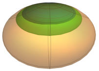
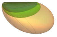
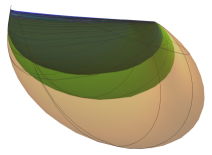
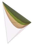
Figure 4. 3-dimensional generalized cusp domains and their foliation by horospheres in projective space. From left to right, top to bottom the domains are $\Omega(0,0,0)$, $\Omega(1,0,0)$, $\Omega(1,1,0)$, finally $\Omega(1,1,1)$ is shown inside a simplex

The radial flow Equation (1.12) is a one-parameter affine group $\Phi^{\psi}$ that centralizes $T(\psi)$, and $\Phi^{\psi}$-orbits give a foliation by a pencil of lines transverse to the horospheres. The enlarged translation group, Equation (1.30), is $T_{\bf t}=T(\psi)\oplus\Phi^{\psi}\cong{\mathbb{R}}^{3}$. It is obtained by replacing the most complicated term in the matrix for $T(\psi)$ by $z$. There are 4 such groups, depending only on ${\bf t}$. Then $T_{\psi}$ is the kernel of a homomorphism $T_{\bf t}\to{\mathbb{R}}$ obtained from $\psi$. The group $T({\bf t})$ acts simply transitively on ${\mathbb{R}}_{+}^{\color[rgb]{0,0,0}{\bf t}}\times{\mathbb{R}}^{3-\color[rgb]{0,0,0}{\bf t}}$, and the latter contains $\Omega(\psi)$.

The group, $O(\psi)$, is the subgroup of $G(\psi)$ that fixes the basepoint (see Definition (1.9)). It is computed in Proposition 1.44, and $O(0,0,0)\cong O(2)$, and $O(\psi_{1},0,0)\cong O(1)$ when $\psi_{1}\neq 0$. For the remaining cases, $O(\psi)$ is the group of coordinate permutations of ${\mathbb{R}}^{3}$ that preserve $\psi$. In particular $O(\psi)$ is finite unless $\psi=0$.

There is a 6 parameter family of marked, 3-dimensional generalized cusps. As described in Theorem 0.2 they are parameterized by a triple $(\psi,\Gamma,A\cdot O(\psi))$ with $\psi$ as above, and $\Gamma$ is a marked lattice of co-area $1$ in ${\mathbb{R}}^{2}$, and $A\cdot O(\psi)\in O(2)/O(\psi)$ is a left coset.

In [25], the third author showed that in dimension 3, every translation group, as defined in Definition 3.9, is conjugate into one of these 4 families. This, together with [1], provided the impetus for the present paper.

We now describe some geometric properties of these domains and discuss relevant examples from the literature. The interior of $\Omega(0,0,0)$ is projectively equivalent to ${\mathbb{H}}^{3}$. If $C\cong\Omega(0,0,0)/\Gamma$ then $\Gamma$ is conjugate into $\operatorname{PO}(3,1)$. Cusps of finite volume hyperbolic 3-manifolds give rise to generalized cusps of this type. The ideal boundary, see Equation (1.23), of $\Omega(0,0,0)$ consists of a single point which is stabilized by $G(\psi)$, and $C$ admits a compactification by a singular projective manifold obtained by adjoining this ideal boundary point.

For a generalized cusp $C=\Omega/\Gamma_{C}$ modelled on $\Omega=\Omega(1,0,0)$ the ideal boundary, $\partial_{\infty}\Omega$ is a projective line segment $J$. The action of $\Gamma_{C}$ on $I=\operatorname{int}(J)$ is discrete iff $\Gamma$ contains a parabolic. In this case $C$ has a compactification $\overline{C}=(\Omega\cup I)/\Gamma_{C}$ that is a projective manifold that is singular along the circle $S^{1}=I/\Gamma_{C}$.

In [1], the first author found, for $t\in[0,\infty)$, a continuous family of properly convex manifolds projectively equivalent to $M_{t}=\Omega_{t}/\Lambda_{t}$, and diffeomorphic to the figure-8 knot complement, $X=S^{3}\setminus K$, and $M_{0}$ is the complete hyperbolic structure. Moreover the end of $M_{t}$ is projectively equivalent to $\Omega(t,0,0)/\Gamma_{t}$, where $\Gamma_{t}\subset T(t,0,0)$ is a lattice containing parabolics. As a result, for $t>0$, there is a compactification $\overline{M}(t)=\Omega^{+}_{t}/\Lambda_{t}$ that is a projective structure on $S^{3}$ that is singular along $K$, and $M_{t}=\overline{M}(t)\setminus K$ is a properly convex structure on $X$. Here $\Omega^{+}_{t}\supset\Omega_{t}$ and also contains the $\Gamma_{t}$-orbit of an open segment in $\partial_{\infty}\Omega(t,0,0)$. The cusp of the hyperbolic manifold $M_{0}$ deforms to a generalized cusp of a different type. As the deformation proceeds, an ideal boundary point of ${\mathbb{H}}^{3}$ opens up into an ideal boundary segment. This is an example of a geometric transition; the hyperbolic cusp $\Omega(0,0,0)/\Gamma_{0}$ geometrically transitions to the non-hyperbolic cusp $\Omega(t,0,0)/\Gamma_{t}$ as $t$ moves away from zero, cf. [18] and [15]. Higher dimensional examples of hyperbolic manifolds deforming to properly convex manifolds with type 1 cusps can be found in [4]. Furthermore, in subsequent work, the authors will show that every generalized cusp arises as a deformation of a hyperbolic cusp in this way.

The domains of the form $\Omega(\psi_{1},\psi_{2},0)$ have ideal boundary a 2-simplex, $\Delta$. The interior of one of the edges of $\Delta$ consists of $C^{1}$ points, and the remainder of the 1-skeleton of $\Delta$ consists of non-$C^{1}$ points. In particular, the fixed point of the radial flow is the intersection of the two edges of non-$C^{1}$ points of $\Delta$, see Lemma 1.29. Any lattice in $T(\psi_{1},\psi_{2},0)$ acts properly discontinuously on $\Delta$. Thus $C=\Omega(\psi_{1},\psi_{2},0)/\Gamma$ has a manifold compactification by adjoining $\Delta/\Gamma$. Recently, Martin Bobb produced the first examples of hyperbolic 3-manifolds with type 2 cusps [6]. Roughly speaking, his examples are constructed by starting with a certain arithmetic hyperbolic 3-manifold and successively bending along a pair of orthogonal totally geodesic hypersurfaces. The first author has also been able to show, using different techniques, that there are infinitely many hyperbolic 1 cusped hyperbolic 3-manifolds that admit properly convex structures with type 2 cusps (see [2]).

Finally, the domains of the form $\Omega(\psi_{1},\psi_{2},\psi_{3})$ also have ideal boundary consisting of a 2-simplex $\Delta$. However, in this case each point of the 1-skeleton of $\Delta$ is a non-$C^{1}$ point. As in the previous case, if $\Gamma$ is a lattice in $T(\psi_{1},\psi_{2},\psi_{3})$ then $\Gamma$ acts properly discontinuously on $\Delta$ and there is a compactification of $C$ by adjoining $\Delta/\Gamma$. There are examples of properly convex deformations of the complete hyperbolic structure on finite volume hyperbolic 3-manifolds whose topological ends are of the form $\Omega(\psi_{1},\psi_{2},\psi_{3})/\Gamma$, where $\Gamma\leq T(\psi_{1},\psi_{2},\psi_{3})$. The first such examples were constructed by Benoist [5] using Coxeter orbifolds. These ideas were extended and generalized by Marquis in [27] allowing him to construct further examples. Other examples were constructed for the figure-eight knot complement and the figure-eight sister by Gye-Seon Lee [24]. His examples are constructed by gluing together two projective ideal tetrahedra using the combinatorial pattern that produces the figure-eight knot complement (see Chapter 3 of [33] for details). Subsequent work of the first author, J. Danciger and G-S. Lee showed that any finite volume hyperbolic 3-manifold that satisfies a mild cohomological condition (that is known to be satisfied by infinitely many hyperbolic 3-manifolds, (for example, by applying [23], Theorem 1.4 to the Whitehead link) also admits deformations all of whose ends are projectively equivalent to $\Omega(1,1,1)/\Gamma$, where $\Gamma\leq T(1,1,1)$, thus producing many additional examples.

Furthermore, as explained in Section 1.4, the lack of $C^{1}$ points in the 1-skeleton of the ideal boundary allows properly convex manifolds with ends projectively equivalent to quotients of $\Omega(\psi_{1},\psi_{2},\psi_{3})$ to sometimes be glued together to produce new properly convex manifold. This idea is explored in detail in [3] and using these techniques it is possible to find properly convex projective structures on non-hyperbolic 3-manifolds. This was first done by Benoist [5] using Coxeter orbifolds.

References

- [1] Ballas, S. Finite Volume properly-convex Deformations of the Figure-Eight Knot Geom. Dedicata 178 (2015), 49-73
- [2] Ballas, S. Constructing convex projective 3-manifolds with generalized cusps Preprint May 2018. https://arxiv.org/abs/1805.09274
- [3] Ballas, S., Danciger, J., and Lee, G. Convex Projective Structures on Non-Hyperbolic 3-Manifolds Geometry and Topology 22 (2018) p. 1593–1646
- [4] Ballas, S. and Marquis, L., Properly Convex Bending of Hyperbolic Manifolds Preprint September 2016. https://arxiv.org/pdf/1609.03046.pdf
- [5] Benoist, Yves, Convexes divisibles. IV. Structure du bord en dimension 3, Invent. Math. ,164, (2)249-278, (2006)
- [6] Bobb, Martin, Convex projective manifolds with a cusp of any non-diagonalizable type Preprint August 2018. https://arxiv.org/abs/1808.02779
- [7] Burago, D., Burago, Y., and Ivanov, S., A course in metric gemetry, Graduate Studies in Mathematics, Vol 33, Amer. Math. Soc., 2001
- [8] Busemann, Herbert, Intrinsic area Ann. of Math. (2) vol(48) 234-267, (1947)
- [9] Calabi, Eugenio, Hypersurfaces with maximal affinely invariant area Amer. J. Math. 104 (1982) 91-126
- [10] Charlap, L. Bieberbach groups and flat manifolds Springer-Verlag, (1986)
- [11] Choi, S. A Classification of Radial or Totally Geodesic Ends of Real Projective Orbifolds I: A Survey of Results. Advanced Studies in Pure Mathematics, Vol. 73 (2017), 69-134, MSJ, Tokyo, Japan, arXiv:1501.00348
- [12] Choi, S., Real projective orbifolds with ends and their deformation theory, a book draft http://mathsci.kaist.ac.kr/~schoi/bookAMSI_ver2_06142018ii.pdf
- [13] S. Choi, G. Lee, and L. Marquis. Deformations of convex real projective structures on manifolds and orbifolds. Survey for the Handbook of Group Actions edited by Lizhen Ji, Athanase Papadopoulos and Shing-Tung Yau
- [14] Cooper, D. The Heisenberg group acts on a strictly convex domain. Conformal Geometry and Dynamics 21 (2017) 101-104
- [15] Cooper, D., Danciger, J., and Wienhard, A. Limits of Geometries. Trans. Amer. Math. Soc. 370 (2018) 6585-6627
- [16] Cooper, D., Long, D., and Tillmann, S. On Convex Projective Manifolds and Cusps. Advances in Mathematics 277 (2015), 181-251.
- [17] Cooper, D., Long, D., and Tillmann, S., Deforming Convex Projective Manifolds, Geom. Topol. 22 (2018) no 3, 1349-1404
- [18] Danciger, J. A geometric transition from hyperbolic to anti-de Sitter geometry, Geom. Topol. 17 (2013) (5) ,3077-3134
- [19] Danciger, J., Kassel, F., and Guéritaud, F. Convex Cocompact Actions in Real Projective Geometry 2017 https://arxiv.org/pdf/1704.08711.pdf
- [20] Goldman, W. Projective Geometry on Manifolds. http://www.math.umd.edu/wmg/gstom.pdf
- [21] Goldman, W. Convex real projective structures on compact surfaces. J. Differential Geom 31, (1990) (3), 791-845
- [22] P. de la Harpe. On Hilbert’s metric for simplices. In Geometric group theory, Vol. 1 (Sussex, 1991), volume 181 of London Math. Soc. Lecture Note Ser., pages 97–119. Cambridge Univ. Press, Cambridge, 1993.
- [23] Heusener, M., and Porti, J., Infinitesimal Projective Rigidity Under Dehn Filling Geom. Topol. Vol. 15, Number 4 (2011), 2017-2071.
- [24] Lee, G.-S., Personal Communication
- [25] Leitner, A. A Classification of Subgroups of Isomorphic to and Generalized Cusps in Projective 3-Manifolds. Topology and its Applications 206, (2016), 241-254
- [26] Marquis, L. Espaces des modules des surfaces projectives proprement convexes de volume fini. Geometry and topology 14, (2010), p. 2103-2149
- [27] Marquis, L. Espace des modules de certains polyèdres projectifs miroirs. Geom. Dedicata 147 (2010), p. 47–86.
- [28] Marquis, L. Surface projective proprement convexe de volume fini. Annales de l’institut Fourier 62, 1 (2012), p. 325-392.
- [29] Marquis, L. Around Groups in Hilbert Geomety. In A Handbook of Hilbert Geometry, eds Papadopoulos, A., and Troyanov, M. IRMA Lectures in Mathematics and Theoretical Physics (22) 2014 p.207-261.
- [30] Shima, H. Homogeneous Hessian manifolds Ann. Inst. Fourier (Grenoble), 30 (1980) 3, 91-128
- [31] E. Socié-Méthou. Behaviour of distance functions in Hilbert-Finsler geometry. Differential Geom. Appl., 20(1):1–10, 2004.
- [32] Schneider, R. Closed convex hypersurfaces with second fundamental form of positive curvature. Proc. Amer. Math. Soc., 35, 1972, 230-233.
- [33] Thurston, W. The Geometry and Topology of Three-Manifolds. Princeton Univ. Math. Dept. Available from http://msri.org/publications/books/gt3m/, 1979.