Site-Occupation Embedding Theory using Bethe Ansatz Local Density Approximations

Abstract

Site-occupation embedding theory (SOET) is an alternative formulation of density-functional theory (DFT) for model Hamiltonians where the fully-interacting Hubbard problem is mapped, in principle exactly, onto an impurity-interacting (rather than a non-interacting) one. It provides a rigorous framework for combining wavefunction (or Green function) based methods with DFT. In this work, exact expressions for the per-site energy and double occupation of the uniform Hubbard model are derived in the context of SOET. As readily seen from these derivations, the so-called bath contribution to the per-site correlation energy is, in addition to the latter, the key density-functional quantity to model in SOET. Various approximations based on Bethe ansatz and perturbative solutions to the Hubbard and single impurity Anderson models are constructed and tested on a one-dimensional ring. The self-consistent calculation of the embedded impurity wavefunction has been performed with the density matrix renormalization group method. It has been shown that promising results are obtained in specific regimes of correlation and density. Possible further developments have been proposed in order to provide reliable embedding functionals and potentials.

I Introduction

Although the independent-particle picture is applicable to many electronic systems, such as conventional metals and band insulators, it drastically fails when electron correlation becomes strong, like in transition metal oxides where metal-insulator transitions occur. Describing such a transition accurately at the computational cost of an independent-particle theory is still a challenge. In the context of density-functional theory (DFT), a correction based on the on-site two-electron repulsion parameter $U$ can be explicitly added to the exchange-correlation functional, in the spirit of hybrid functionals, thus leading to the so-called DFT+$U$ method  Anisimov et al. (1991); Liechtenstein et al. (1995). But still, some crucial aspects are missing in the DFT+$U$, for instance strongly-correlated phenomena such as the Kondo effect, which cannot be treated within a static mean-field approximation. Therefore, it is necessary to consider a many-body picture of the problem.

Because it often appears that the region of interest is only one part of a much larger system and considering strong electron correlation as essentially local Pulay (1983); Saebo and Pulay (1993); Hampel and Werner (1996), embedding approaches are mainly used in practice Sun and Chan (2016). In these approaches, the whole system is usually mapped onto an embedded quantum problem, e.g. a small system called impurity and the rest of the system called the bath Ayral et al. (2017). The dynamical mean-field theory (DMFT) Georges and Kotliar (1992); Georges et al. (1996); Kotliar and Vollhardt (2004); Held (2007); Zgid and Chan (2011) has been proved to treat efficiently systems with $d$ or $f$ localized shells, however, there are still some cases for which DMFT is not sufficiently accurate, especially in the case when non local electron correlation becomes important. In order to further improve on its performance, combined DMFT+DFT Kotliar et al. (2006) or DMFT+GW Sun and Kotliar (2002); Biermann et al. (2003); Karlsson (2005); Boehnke et al. (2016); Werner and Casula (2016); Nilsson et al. (2017) schemes have been proposed to recover such effects. In another promising approach, the so-called self-energy embedding theory Kananenka et al. (2015); Lan et al. (2015, 2017), strong correlation is not considered as strictly local, which can be appreciable for real compounds. Its applicability to both model and ab-initio Hamiltonians is also appealing. All these embedding techniques are formulated in terms of the (frequency-dependent) one-particle Green function. On the other hand, in the density-matrix embedding theory (DMET) Knizia and Chan (2012, 2013); Bulik et al. (2014); Zheng and Chan (2016); Wouters et al. (2016a, b); Rubin (2016), the embedded fragment (impurity) is described with a high-level wavefunction-based method while the rest of the system is usually treated at the mean-field level. Extensions have been proposed in order to include correlation in the bath Tsuchimochi et al. (2015) or for improving the description of the boundary between the fragment and the bath Welborn et al. (2016).

Turning to DFT, its extension to model Hamiltonians is usually referred to as site-occupation functional theory (SOFT) Chayes et al. (1985); Gunnarsson and Schönhammer (1986); Schönhammer et al. (1995); Capelle and Campo Jr. (2013). In conventional Kohn-Sham (KS) SOFT, the physical fully-interacting many-body problem is mapped onto a noninteracting one by means of a Hartree-exchange-correlation (Hxc) functional of the density (i.e., the sites occupation in this context). The SOFT has been shown to give very accurate density and energy profiles with the Bethe ansatz local density approximation (BALDA)  Lima et al. (2002, 2003); Capelle et al. (2003), the spin-dependent BALDA  Franca et al. (2012), and its fully numerical formulation  Xianlong et al. (2006, 2007). The methods have been applied to both repulsive  Silva et al. (2005); Akande and Sanvito (2010) and attractive  Campo Jr and Capelle (2005); Xianlong (2008) Hubbard models. The electronic transport has also been studied by applying SOFT to the Anderson junction model  Bergfield et al. (2012); Liu et al. (2012); Liu and Burke (2015). Time-dependent Verdozzi (2008); Kurth et al. (2010); Karlsson et al. (2011) and temperature-dependent extensions Stefanucci and Kurth (2011); Xianlong et al. (2012) have been investigated over the years. Other reduced quantities can also be used, as first discussed by Schönhammer et al. Schönhammer et al. (1995), such as the 1-body reduced density matrix  Schindlmayr and Godby (1995); López-Sandoval and Pastor (2002, 2004); Saubanère and Pastor (2009, 2011); Töws and Pastor (2011); Töws et al. (2014); Saubanère et al. (2016), or the steady current in connection with steady-state transport Stefanucci and Kurth (2015); Kurth and Stefanucci (2016).

For the purpose of modelling strongly correlated regimes, some of the authors have recently proposed an alternative formulation of SOFT where, in contrast to standard KS SOFT, the interacting Hubbard problem is mapped onto an impurity-interacting one, thus leading to an in-principle-exact site-occupation embedding theory (SOET) Fromager (2015); Senjean et al. (2017). In order to turn SOET into a practical computational method, embedding density-functional approximations must be developed. This has been done so far only for the asymmetric Hubbard dimer Senjean et al. (2017). In this work we show how Bethe ansatz and perturbative solutions to both Hubbard and Anderson models can be used for designing local density approximations in the context of SOET. In Ref. Senjean et al. (2017), the self-consistent impurity problem SOET relies on was solved for a 8-site model by exact diagonalization, as a proof of concept. In this work, we also present an implementation of SOET where the embedded impurity system is treated with the density matrix renormalization group (DMRG) method  White (1992, 1993); Verstraete et al. (2008); Schollwöck (2011); Nakatani , thus allowing for calculations on larger rings.

The paper is organized as follows. After a brief review of SOET (Sec. II.1), exact SOET-based expressions for the per-site energy and double occupation are derived in Sec. II.2, in the particular case of the uniform one-dimensional Hubbard problem. Exact properties of the embedding functionals are also presented. The construction of local density-functional approximations is then discussed in Sec. II.3. A connection between SOET and the single impurity Anderson model is investigated in Sec. II.4. A summary of the various approximations tested in this work is given in Sec. III with the computational details. The results are discussed in Sec. IV. Conclusions and perspectives are finally given in Sec. V.

II Theory

II.1 Site occupation embedding theory

We focus on the one-dimensional Hubbard model in an external potential $\mathbf{v}\equiv\{v_{i}\}_{i}$,

$$\hat{H}(\mathbf{v})=\hat{T}+\hat{U}+\hat{V},$$ (1)

where the hopping operator,

$$\hat{T}=-t\sum_{i=0}^{L-1}\sum_{\sigma=\uparrow,\downarrow}\left(\hat{c}^{\dagger}_{i\sigma}\hat{c}_{i+1\sigma}+\mathrm{H.c.}\right),$$ (2)

is the analog of the kinetic energy operator in ab-initio Hamiltonians. Here $t$ is the hopping integral and $\hat{c}_{i\sigma}^{\dagger}$ is the creation operator of an electron at the $i$th site with spin $\sigma=\uparrow,\downarrow$. The site index $i$ runs from $0$ to $L-1$ where $L$ is the number of sites, and we impose the periodic boundary condition $\hat{c}_{L\sigma}=\hat{c}_{0\sigma}$. The on-site two-electron repulsion operator is given by

$$\hat{U}=U\sum_{i=0}^{L-1}\hat{n}_{i\uparrow}\,\hat{n}_{i\downarrow},$$ (3)

where $\hat{n}_{i\sigma}=\hat{c}_{i\sigma}^{\dagger}\hat{c}_{i\sigma}$ and $U$ represents the Hubbard interaction between spin-up and spin-down electrons on the same site. In order to formulate the SOFT and SOET, we further introduce the on-site potential operator by

$$\hat{V}=\sum_{i=0}^{L-1}v_{i}\,\hat{n}_{i},$$ (4)

where $\hat{n}_{i}=\hat{n}_{i\uparrow}+\hat{n}_{i\downarrow}$. In order to have a self-contained paper, this subsection summarizes the main equations of Ref. Senjean et al. (2017).

In SOFT, the exact ground-state energy is obtained variationally as

$$E(\mathbf{v})=\underset{\mathbf{n}}{\rm min}\left\{F(\mathbf{n})+(\mathbf{v}|\mathbf{n})\right\},$$ (5)

where $\mathbf{n}\equiv\{n_{i}\}_{i}$ is the site-occupation (simply called density in the following) vector and $(\mathbf{v}|\mathbf{n})=\sum_{i}v_{i}n_{i}$. The Levy–Lieb (LL) functional reads

$$F(\mathbf{n})=\underset{\Psi\rightarrow\mathbf{n}}{\rm min}\left\{\langle\Psi|\hat{T}+\hat{U}|\Psi\rangle\right\},$$ (6)

where the minimization is restricted to wavefunctions $\Psi$ with density $\mathbf{n}$.

In the conventional KS formalism, the LL functional is decomposed as

$$F(\mathbf{n})=T_{\rm s}(\mathbf{n})+E_{\rm Hxc}(\mathbf{n}),$$ (7)

where $T_{\rm s}(\mathbf{n})=\underset{\Psi\rightarrow\mathbf{n}}{\rm min}\{\langle\Psi|\hat{T}|\Psi\rangle\}$ is the $t$-dependent analog of the noninteracting kinetic energy functional and

$$E_{\rm Hxc}(\mathbf{n})=\dfrac{U}{4}\sum_{i}n_{i}^{2}+E_{\rm c}(\mathbf{n})$$ (8)

is the $t$- and $U$-dependent Hxc functional. The latter is “universal” in a sense that it does not depend on the external potential $\mathbf{v}$.

Turning to the SOET Fromager (2015); Senjean et al. (2017), we label, for convenience, the location of the “to be embedded” impurity site in real (discretized) space as $i=0$. The LL functional is then decomposed into impurity and bath contributions as

$$F(\mathbf{n})=F^{\rm imp}(\mathbf{n})+\overline{E}_{\rm Hxc}^{\rm bath}(\mathbf{n}),$$ (9)

where the impurity-interacting LL functional reads

$$F^{\rm imp}(\mathbf{n}) = \underset{\Psi\rightarrow\mathbf{n}}{\rm min}\left\{\langle\Psi|\hat{T}+\hat{U}_{0}|\Psi\rangle\right\},$$ (10)

with $\hat{U}_{0}=U\hat{n}_{0\uparrow}\hat{n}_{0\downarrow}$. By using Eqs. (5), (9), and (10), we obtain the exact SOET energy expression Fromager (2015); Senjean et al. (2017),

$$E(\mathbf{v})=\underset{\Psi}{\rm min}\left\{\langle\Psi|\hat{T}+\hat{U}_{0}|\Psi\rangle+\overline{E}^{\rm bath}_{\rm Hxc}(\mathbf{n}^{\Psi})+(\mathbf{v}|\mathbf{n}^{\rm\Psi})\right\},$$ (11)

where $\mathbf{n}^{\rm\Psi}\equiv\{\langle\Psi|\hat{n}_{i}|\Psi\rangle\}_{i}$ is the density of the trial many-body wavefunction $\Psi$. The optimized impurity-interacting wavefunction $\Psi^{\rm imp}$ in Eq. (11) fulfills the following self-consistent equation,

$$\displaystyle\left(\hat{T}+\hat{U}_{0}+\displaystyle\sum_{i}\left[v_{i}+\dfrac{\partial\overline{E}^{\rm bath}_{\rm Hxc}(\mathbf{n}^{\Psi^{\rm imp}})}{\partial n_{i}}\right]\hat{n}_{i}\right)|\Psi^{\rm imp}\rangle$$

$$=\mathcal{E}^{\rm imp}|\Psi^{\rm imp}\rangle,$$ (12)

where $\{{v_{i}+\partial\overline{E}^{\rm bath}_{\rm Hxc}(\mathbf{n}^{\Psi^{\rm imp}})/\partial n_{i}\}}_{i}$ plays the role of an embedding potential for the impurity. This potential is unique (up to a constant) and ensures, like the KS potential in conventional DFT, that $\Psi^{\rm imp}$ reproduces the exact ground-state density of the true (fully-interacting) Hubbard Hamiltonian. Any correlated method based on the explicit calculation of many-body wavefunctions or Green functions could in principle be applied for solving Eq. (II.1). Obviously, in order to perform practical SOET calculations, it is necessary to develop approximations to the complementary bath functional introduced in Eq. (9). This is the main focus of this paper. Let us first consider the following KS decomposition of Eq. (10),

$$F^{\rm imp}(\mathbf{n})=T_{\rm s}(\mathbf{n})+E^{\rm imp}_{\rm Hxc}(\mathbf{n}),$$ (13)

where

$$E^{\rm imp}_{\rm Hxc}(\mathbf{n})=\dfrac{U}{4}n_{0}^{2}+E^{\rm imp}_{\rm c}(\mathbf{n})$$ (14)

is the analog of the Hxc functional for the impurity-interacting system. By combining Eqs. (9) and (13), we have

$$\overline{E}_{\rm Hxc}^{\rm bath}(\mathbf{n})=\dfrac{U}{4}\sum_{i\neq 0}n_{i}^{2}+\overline{E}_{\rm c}^{\rm bath}(\mathbf{n}),$$ (15)

where the exact correlation functional for the bath,

$$\overline{E}_{\rm c}^{\rm bath}(\mathbf{n})=E_{\rm c}(\mathbf{n})-E_{\rm c}^{\rm imp}(\mathbf{n}),$$ (16)

is simply the difference in correlation energy between the fully-interacting system (i.e., an interacting impurity site surrounded by interacting bath sites), for which local density-functional approximations have already been developed (see, for example, Refs. Lima et al. (2003); Xianlong et al. (2012)) and the auxiliary system consisting of an interacting impurity site surrounded by non-interacting bath sites, both systems having the same density $\mathbf{n}$. In the rest of this work we will discuss various strategies for developing local density functional approximations to $\overline{E}_{\rm c}^{\rm bath}(\mathbf{n})$ or, equivalently, $E_{\rm c}(\mathbf{n})$ and $E_{\rm c}^{\rm imp}(\mathbf{n})$. For that purpose, we will first derive in the next section exact properties of the latter functionals for a uniform system.

II.2 Exact SOET for the uniform Hubbard model

Following Capelle and coworkers Lima et al. (2002), we will use as reference the uniform Hubbard system ($\mathbf{v}=\mathbf{0}$) in the following in order to derive local density approximations for $\overline{E}_{\rm c}^{\rm bath}(\mathbf{n})$. In this context, the standard density-functional correlation energy Lima et al. (2003),

$$E_{\rm c}(\mathbf{n})=\sum_{i}e_{\rm c}(n_{i}),$$ (17)

is simply expressed in terms of the per-site correlation energy $e_{\rm c}(n)$ for which an exact analytical expression can be obtained at half-filling from the Bethe ansatz Lieb and Wu (1968). For convenience, we introduce the per-site analog of Eq. (16),

$$\overline{e}_{\rm c}^{\rm bath}(\mathbf{n})=e_{\rm c}(n_{0})-E_{\rm c}^{\rm imp}(\mathbf{n}),$$ (18)

which leads to the final expression,

$$\overline{E}_{\rm c}^{\rm bath}(\mathbf{n}) = \sum_{i\neq 0}e_{\rm c}(n_{i})+\overline{e}_{\rm c}^{\rm bath}(\mathbf{n}).$$ (19)

Let us stress that the deviation of the impurity correlation energy $E_{\rm c}^{\rm imp}(\mathbf{n})$ from the conventional (total) per-site correlation energy $e_{\rm c}(n_{0})$ is the key density-functional quantity to model in the SOET. It becomes even more clear when considering, for example, the exact (uniform) double site-occupation expression Capelle and Campo Jr. (2013)

$$d=\langle\hat{n}_{i\uparrow}\hat{n}_{i\downarrow}\rangle=\dfrac{1}{L}\dfrac{\partial E}{\partial U}=\dfrac{n^{2}}{4}+\dfrac{\partial e_{\rm c}(n)}{\partial U},$$ (20)

where $n$ denotes the uniform density in the reference Hubbard system with total energy $E=E({\mathbf{v}=\mathbf{0}})$. As shown in Appendix A, the following equivalent expression is obtained in SOET,

$$d = d^{\rm imp}+\dfrac{\partial\overline{e}_{\rm c}^{\rm bath}(\mathbf{n}^{\Psi^{\rm imp}})}{\partial U},$$ (21)

where $d^{\rm imp}=\langle\Psi^{\rm imp}|\hat{n}_{0\uparrow}\hat{n}_{0\downarrow}|\Psi^{\rm imp}\rangle$ is the double occupation of the impurity site for the impurity-interacting wavefunction $\Psi^{\rm imp}$. Note that, in the exact theory, the latter is expected to reproduce the uniform density only (i.e., $\underline{n}\equiv\big{\{}n_{i}=n\big{\}}_{i}\equiv\mathbf{n}^{\Psi^{\rm imp}}$) and not the double occupation, hence the second density-functional contribution on the right-hand side of Eq. (21). Turning to the per-site energy Lima et al. (2003),

$$e=\frac{E}{L}=t_{\rm s}(n)+\dfrac{U}{4}n^{2}+e_{\rm c}(n),$$ (22)

where $t_{\rm s}(n)=-4t\sin(\pi n/2)/\pi$ in the thermodynamic limit ($L\rightarrow+\infty$), we equivalently obtain in SOET (see the proof in Appendix B) the following exact expression,

$$e = t_{\rm s}(n^{\Psi^{\rm imp}}_{0})+Ud^{\rm imp}+t\dfrac{\partial e_{\rm c}(n^{\Psi^{\rm imp}}_{0})}{\partial t}+\overline{e}_{\rm c}^{\rm bath}(\mathbf{n}^{\Psi^{\rm imp}})$$ (23)

$$-t\dfrac{\partial\overline{e}_{\rm c}^{\rm bath}(\mathbf{n}^{\Psi^{\rm imp}})}{\partial t}.$$

In contrast to the regular KS expressions [Eqs. (20) and (22)], our SOET expressions [Eqs. (21) and (23)] involve the (embedded impurity) double occupation explicitly, which can improve on the results significantly when approximate density functionals are used, as shown in Sec. IV.

Returning to the exact theory, let us now highlight some properties of $\overline{e}_{\rm c}^{\rm bath}(\mathbf{n})$. Since the standard per-site correlation functional as well as the impurity one are invariant under hole-particle symmetry (see Ref. Capelle and Campo Jr. (2013) and Appendix C), the per-site bath correlation functional is also invariant, according to Eq. (18), i.e. $\overline{e}_{\rm c}^{\rm bath}(\mathbf{n})=\overline{e}_{\rm c}^{\rm bath}(\underline{2}-\mathbf{n})$. Consequently, the exact embedding potential in the uniform case [see Eq. (II.1)],

$$\left.\dfrac{\partial\overline{E}^{\rm bath}_{\rm Hxc}(\mathbf{n})}{\partial n_{i}}\right|_{\mathbf{n}=\underline{n}} = (1-\delta_{i0})\left(\dfrac{Un}{2}+\dfrac{\partial e_{\rm c}(n)}{\partial n}\right)$$ (24)

$${}+\left.\dfrac{\partial\overline{e}_{\rm c}^{\rm bath}(\mathbf{n})}{\partial n_{i}}\right|_{\mathbf{n}=\underline{n}},$$

will, at half-filling ($n=1$) and for a finite-size system, be equal to $U/2$ everywhere in the bath and zero on the impurity site or, equivalently, $-U/2$ on the impurity site and zero in the bath (see Appendix C). In this particular case, the auxiliary impurity-interacting system is similar to the symmetric single-impurity Anderson model (SIAM) Anderson (1961). This feature has already been observed numerically in the particular case of a 8-site ring in Ref. Senjean et al. (2017) but, at the time, it was not rationalized in terms of hole-particle symmetry as we just did. Away from half-filling, the embedding potential loses its uniformity in the bath since the interaction on the impurity site breaks translation symmetry Senjean et al. (2017). This fact, which is the price to pay for achieving an exact embedding, explains why $\overline{e}_{\rm c}^{\rm bath}(\mathbf{n})$ should in principle depend not only on the impurity site occupation but also on the bath site ones [see Eq. (24)]. For simplicity, the latter dependence will be neglected in the following,

$$\overline{e}_{\rm c}^{\rm bath}(\mathbf{n})\rightarrow\overline{e}_{\rm c}^{\rm bath}(n_{0}),$$ (25)

or, equivalently [see Eq. (18)],

$$E_{\rm c}^{\rm imp}(\mathbf{n})\rightarrow E_{\rm c}^{\rm imp}(n_{0}),$$ (26)

thus leaving for future work the investigation of bath-occupations-dependent density-functional approximations.

II.3 Local density-functional approximations based on Bethe ansatz solutions

So far, only one density-functional approximation to the impurity correlation energy [referred to as two-level impurity local density approximation (2L-ILDA) in Ref. Senjean et al. (2017)] has been proposed. It is based on the asymmetric Hubbard dimer and provides essentially an approximate density-functional embedding potential that is set to zero in the bath. Since 2L-ILDA does not model the correlation energy of the bath, it cannot be used straightforwardly for calculating per-site energies and double occupations. We propose in the following to use Bethe ansatz solutions to (fully- or impurity-interacting) infinite systems in order to design local density approximations to the per-site bath correlation energy.

II.3.1 Approximation to $e_{\rm c}(n)$

Regarding the fully-interacting Hubbard model, the BALDA Lima et al. (2002, 2003); Capelle et al. (2003) (which is exact in the thermodynamic limit when $U=0$, $U\rightarrow+\infty$, and for all $U$ values when $n=1$) will be used for modeling $e_{\rm c}(n)$. The correlation energy within BALDA reads

$$e_{\rm c}^{\rm BA}(U,t,n) = e^{\rm BA}(U,t,n)-e^{\rm BA}(U=0,t,n)-\dfrac{U}{4}n^{2},$$

where the $U$- and $t$-dependence of the per-site correlation energy will be dropped for convenience, and the per-site energy is given by

$$e^{\rm BA}(n\leq 1)=\dfrac{-2t\beta(U/t)}{\pi}\sin\left(\dfrac{\pi n}{\beta(U/t)}\right),$$ (28)

and

$$e^{\rm BA}(n\geq 1) = e^{\rm BA}(2-n)+U(n-1).$$ (29)

The $U/t$-dependent function $\beta(U/t)$ is determined by solving

$$\dfrac{-2\beta(U/t)}{\pi}\sin\left(\dfrac{\pi}{\beta(U/t)}\right)=-4\int_{0}^{\infty}\frac{dx}{x}\dfrac{J_{0}(x)J_{1}(x)}{1+\exp\left(\frac{U}{2t}x\right)},$$ (30)

where $J_{0}$ and $J_{1}$ are zero and first order Bessel functions. Although this functional has been proved to give accurate energy and density profiles, we show here that it depicts a wrong behaviour around $U=0$ away from the half-filled case, which appears to be important for the calculation of the double occupation in Eq. (20). Indeed, since $\beta(0)=2$ and $\partial\beta(U/t)/\partial U|_{U=0}=-\pi/(8t)$ it comes

$$\left.\dfrac{\partial e^{\rm BA}_{\rm c}(n)}{\partial U}\right|_{U=0} = \dfrac{1}{4}\left[\sin\left(\dfrac{\pi n}{2}\right)-n^{2}\right]-\dfrac{n\pi}{8}\cos\left(\dfrac{\pi n}{2}\right),$$

and, consequently, for $n\leq 1$,

$$\dfrac{\partial}{\partial n}\left.\dfrac{\partial e^{\rm BA}_{\rm c}(n)}{\partial U}\right|_{U=0} = \dfrac{n\pi^{2}}{16}\sin\left(\dfrac{\pi n}{2}\right)-\dfrac{n}{2}.$$ (32)

As readily seen from Eqs. (II.3.1) and (32), away from half-filling, both BALDA correlation energy and potential will vary linearly with $U$ in the weakly-correlated regime, which is of course unphysical. This observation will be important when discussing the performance of BALDA-based functionals for the calculation of per-site energies and double occupations in SOET, as well as for the analysis of so-called density-driven errors (see Sec. IV).

Note that, in the thermodynamic limit, the correlation potential $\partial e_{\rm c}(n)/\partial n$ exhibits a discontinuity at half-filling ($n=1$) so that the exact fundamental gap can be reproduced in KS-SOFT Lima et al. (2002). The BALDA can model such a discontinuity by construction, as it can actually be seen from Eq. (32) when $n=1$, but this leads to convergence problems around the Mott transition phase or in the Coulomb blockade regime. Solutions have been proposed using finite temperature Xianlong et al. (2012) or ad-hoc parameters Kurth et al. (2010); Karlsson et al. (2011); Ying et al. (2014). On the other hand, in exact SOET, the complementary per-site bath correlation potential $\partial\overline{e}_{\rm c}^{\rm bath}(\mathbf{n})/\partial n_{i}$ is not expected to be discontinuous neither on the impurity site, where the two-electron repulsion is treated explicitly, nor in the bath where the standard correlation potential already contains the discontinuity [see Eq. (24)]. This can be easily shown in the atomic limit (see Appendix D).

II.3.2 Approximations to $E_{\rm c}^{\rm imp}(n_{0})$

Turning to density-functional approximations for $\overline{e}_{\rm c}^{\rm bath}(n_{0})$ or, equivalently, $E_{\rm c}^{\rm imp}(n_{0})$, the simplest one [referred to as impurity-BALDA (iBALDA) in the following] consists in modeling the correlation energy of the impurity-interacting system with the BALDA:

$$E_{\rm c}^{\rm imp}(n_{0})\xrightarrow{\rm iBALDA}e_{\rm c}^{\rm BA}(n_{0}).$$ (33)

In other words, the iBALDA neglects the contribution of the bath to the total per-site correlation energy [see Eq. (18)],

$$\overline{e}_{\rm c}^{\rm bath}(n_{0})\xrightarrow{\text{iBALDA}}0.$$ (34)

Despite its apparent simplicity, this approximation will show to be very accurate away from half-filling, but it overestimates the correlation energy of the impurity otherwise. This will be discussed further in Sec. IV. Improvement can be considered either by increasing the number of impurities Fromager (2015) (and still use the iBALDA), in analogy with the DMET Knizia and Chan (2012), or by developing more accurate approximations to $\overline{e}_{\rm c}^{\rm bath}(n_{0})$ while keeping a single impurity site. The latter option is of course preferable in terms of computational cost. It can be implemented, in the half-filled case, by exploiting the already mentioned (see Sec. II.2) analogy between the auxiliary impurity-interacting system and the symmetric SIAM. Using the latter for extracting an approximate $E_{\rm c}^{\rm imp}({n}_{0})$ functional gives, when combined with the BALDA, an approximation that will be referred to as the SIAM-BALDA[$n$=1] in the following,

$$\overline{e}_{\rm c}^{\rm bath}(n_{0}=1) \xrightarrow[{\rm BALDA}[n=1]]{\rm SIAM} e^{\rm BA}_{\rm c}(n_{0}=1)$$ (35)

$$-E^{\rm SIAM}_{\rm c}(U,\Gamma,n_{0}=1),$$

where $\Gamma$ is the impurity level width parameter of the SIAM Georges (2016). For clarity, we postpone to Sec. II.4 the discussion on the choice of $\Gamma$ in the context of SOET. The correlation energy in the symmetric SIAM can be well described in all correlation regimes by a simple interpolation between the weakly and the strongly correlated limits,

$$E^{\rm SIAM}_{\rm c}(U,\Gamma,n=1) = \frac{1}{1+f}E^{\rm SIAM}_{{\rm c},U/\Gamma\rightarrow 0}(U,\Gamma)$$

$${}+\frac{f}{1+f}E^{\rm SIAM}_{{\rm c},U/\Gamma\rightarrow\infty}(U,\Gamma,n=1),$$

where $f=f(U/\Gamma)=e^{U/\Gamma-6.876}$. Here in the weakly correlated limit, we use Yamada’s perturbative expression through fourth order in $U/\Gamma$ Yamada (1975),

$$E^{\rm SIAM}_{{\rm c},U/\Gamma\rightarrow 0}(U,\Gamma)=\dfrac{U^{2}}{\pi\Gamma}\left[-0.0369+0.0008\left(\dfrac{U}{\pi\Gamma}\right)^{2}\right].$$ (37)

Regarding the strongly correlated limit, we propose to use a simplified version of the density-functional approximation developed by Bergfield et al. which relies on the BA solution to the strongly correlated SIAM Bergfield et al. (2012); Liu et al. (2012). An impurity correlation energy functional is obtained by integrating (with respect to the density $n$) the parameterized correlation potential of Eqs. (15) and (16) in Ref. Bergfield et al. (2012), which gives:

$$\begin{array}[]{l}E^{\rm SIAM}_{{\rm c},U/\Gamma\rightarrow\infty}(U,\Gamma,n)=\alpha(U,\Gamma)\dfrac{U}{2}\Big{[}\mathcal{E}_{\rm c}(U,\Gamma,n)-\mathcal{E}_{\rm c}(U,\Gamma,0)\Big{]},\\ \\ \mathcal{E}_{\rm c}(U,\Gamma,n)=n-\dfrac{n^{2}}{2}+\dfrac{2}{\pi}(1-n){\rm tan}^{-1}\left[\dfrac{(1-n)}{\sigma}\right]-\dfrac{\sigma}{\pi}\ln\left[1+\left(\dfrac{(1-n)}{\sigma}\right)^{2}\right],\end{array}$$ (41)

where $\alpha(U,\Gamma)=U/(U+5.68\Gamma)$ and

$$\sigma=0.811\dfrac{\Gamma}{U}-0.39\left(\dfrac{\Gamma}{U}\right)^{2}-0.168\left(\dfrac{\Gamma}{U}\right)^{3}.$$ (42)

Note that, in order to be able to use the interpolation in Eq. (II.3.2) in any regime of correlation, i.e., for all values of $U/\Gamma$, we need to reconsider the parameterization in Eq. (42). Indeed, when passing through $\sigma=0$ or, equivalently, when $U/\Gamma\approx 0.755$, the correlation energy undergoes a jump because of the $\tan^{-1}$ function, as shown in Fig. 1. For this reason, we will use in the SIAM-BALDA[$n$=1] approximation the simpler (and still reasonably accurate) expression,

$$\sigma\xrightarrow[{\rm BALDA}[n=1]]{{\rm SIAM}}\dfrac{8\Gamma}{\pi^{2}U},$$ (43)

which originates from the BA solution as $U\rightarrow+\infty$ Bergfield et al. (2012). Note that, with this choice, $E^{\rm SIAM}_{{\rm c},U/\Gamma\rightarrow\infty}(U,\Gamma,n=1)$ becomes positive for smaller $U/\Gamma$ values, which is of course unphysical. This artefact is actually removed by the interpolation in Eq. (II.3.2), as shown in Fig. 1. The numerical value $6.876$ in the interpolation function $f$ simply corresponds to the crossing point between Yamada’s [Eq. (37)] and modified Bergfield’s [Eqs. (41) and (43)] approximate correlation energies.

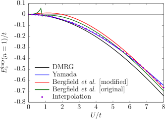
Figure 1: Correlation energy of the embedded impurity for the half-filled 32-site one-dimensional Hubbard model. Various approximations are tested for $\Gamma=t$ [see Sec. II.4]: Eq. (37) [blue curve], Eq. (41) combined with Eq. (42) [green curve], and Eq. (41) combined with Eq. (43) [red curve]. The interpolation SIAM-BALDA[$n$=1] relies on [Eq. (LABEL:eq:inter_siam_func) combined with Eq. (43)] is shown with points in purple. The accurate DMRG result [see Ref. Senjean et al. (2017) for further details about the accurate calculation of correlation energies] is shown in black for comparison.

II.4 Connecting SOET to the SIAM

In order to use density-functional approximations based on the SIAM in the context of SOET we need to relate the impurity level width parameter $\Gamma$ of the SIAM to the parameters of the (original) Hubbard problem $t$ and $U$, and, possibly, the density. This is the purpose of this section. Let us start with the expression for the Hamiltonian of the symmetric SIAM written in (discretized) real space,

$$\hat{H}^{\rm SIAM} = -t\sum_{\sigma}\sum^{L}_{i=1}\left(\hat{c}^{\dagger}_{i\sigma}\hat{c}_{i+1\sigma}+\mathrm{H.c.}\right)$$ (44)

$$+V\sum_{\sigma}\left(\hat{c}^{\dagger}_{1\sigma}\hat{d}_{\sigma}+\hat{c}^{\dagger}_{L\sigma}\hat{d}_{\sigma}+\mathrm{H.c.}\right)$$

$$+U\hat{n}_{d\uparrow}\hat{n}_{d\downarrow}-\dfrac{U}{2}\hat{n}_{d},$$

where we denote $\hat{d}_{\sigma}=\hat{c}_{0\sigma}$, $\hat{n}_{d\sigma}=\hat{d}^{\dagger}_{\sigma}\hat{d}_{\sigma}$, and $\hat{n}_{d}=\sum_{\sigma}\hat{n}_{d\sigma}$. We assume the periodic boundary condition in the bath $\hat{c}_{L+1\sigma}=\hat{c}_{1\sigma}$. As discussed in Sec. II.2, in the particular case of a half-filled $(L+1)$-site Hubbard problem, the exact auxiliary impurity-interacting Hamiltonian of SOET is essentially the one in Eq. (44) if

$$V=-t.$$ (45)

Note that, in principle, we should remove the coupling term between the two neighbors ($i=1$ and $i=L$) of the impurity site. The latter point is ignored in the following for simplicity. Using the representation of bath creation operators in $k$-space,

$$\hat{c}^{\dagger}_{i\sigma}=\frac{1}{\sqrt{L}}\sum_{k}e^{-{\rm i}ki}\hat{c}^{\dagger}_{k\sigma},$$ (46)

with

$$k=\frac{2\pi}{L}m\quad\left(m=-\frac{L}{2}+1,\ldots,\frac{L}{2}\right),$$ (47)

we recover from Eq. (44) the usual SIAM Hamiltonian expression,

$$\hat{H}^{\rm SIAM} = \sum_{k\sigma}\varepsilon_{k}\hat{c}^{\dagger}_{k\sigma}\hat{c}_{k\sigma}+U\hat{n}_{d\uparrow}\hat{n}_{d\downarrow}-\dfrac{U}{2}\hat{n}_{d}$$ (48)

$$+\sum_{k\sigma}\Big{(}V(k)\hat{c}^{\dagger}_{k\sigma}\hat{d}_{\sigma}+\mathrm{H.c.}\Big{)},$$

where $\varepsilon_{k}=-2t\cos k$ and

$$V(k)=\frac{2V}{\sqrt{L}}\,e^{-{\rm i}k/2}\,\cos(k/2)$$ (49)

is the $k$-dependent coupling term between the bath and the impurity. The correlation energy of the impurity is then determined from the frequency-dependent hybridization function Georges (2016)

$$\Gamma(\omega)=\pi\sum_{k}|V(k)|^{2}\delta(\omega-\varepsilon_{k}),$$ (50)

which, according to Eqs. (47) and (49), can be simplified as follows in the thermodynamic limit ($L\rightarrow+\infty$),

$$\Gamma(\omega) = \dfrac{L}{2}\int^{\pi}_{-\pi}dk|V(k)|^{2}\delta(\omega-\varepsilon_{k})$$ (51)

$$= 4V^{2}\int^{\pi}_{0}dk\,\cos^{2}(k/2)\delta(\omega-\varepsilon_{k})$$

$$= \dfrac{V^{2}}{t^{2}}\int^{2t}_{-2t}d\varepsilon\dfrac{t-\dfrac{\varepsilon}{2}}{\sqrt{1-\dfrac{\varepsilon^{2}}{4t^{2}}}}\delta(\omega-\varepsilon).$$

The (frequency-independent) impurity level width parameter $\Gamma$ of the SIAM is usually defined as the value of the hybridization function at the Fermi level $\varepsilon_{F}=-2t\,\cos k_{F}$,

$$\Gamma=\Gamma(\varepsilon_{F})=\dfrac{V^{2}}{t^{2}}\dfrac{t-\dfrac{\varepsilon_{F}}{2}}{\sqrt{1-\dfrac{\varepsilon_{F}^{2}}{4t^{2}}}}.$$ (52)

By using Eq. (45) and the relation between the uniform density $n=N/L$ in the bath and $k_{F}$,

$$N=2\cdot\frac{L}{2\pi}\int_{-k_{F}}^{k_{F}}dk,$$ (53)

or, equivalently,

$$n=\frac{2}{\pi}k_{F},$$ (54)

we finally obtain a $t$-dependent density-functional impurity level width which connects the SIAM to the original Hubbard problem to be solved in SOET:

$$\Gamma=\Gamma(t,n) = t\left(\frac{1+\cos(\pi n/2)}{\sin(\pi n/2)}\right).$$ (55)

Note that the latter expression is valid when $0\leq n\leq 1$. In the range $1\leq n\leq 2$, we should use the hole-particle symmetry relation $\Gamma(t,n)=\Gamma(t,2-n)$.

As readily seen from Eq. (55), we obtain $\Gamma=t$ for the half-filled Hubbard problem ($n=1$). This is the reason why, in Sec. IV, per-site correlation energies have been computed for the bath at the SIAM-BALDA[$n$=1] level of approximation (see Eq. (35)) with $\Gamma$ set to $t$. The deviation from half-filling in the original Hubbard system will be interpreted, in the SIAM, as a rescaling of $\Gamma$. In the low-density regime we have $\Gamma(t,n)\approx 4t/(\pi n)\gg\Gamma(t,n=1)$, thus leading to weaker correlation effects on the embedded impurity site, in comparison to the half-filled case. Consequently, we might expect the simple combination of Yamada’s perturbation expansion in $U/\Gamma$ [see Eq. (37)] with Eq. (55) to provide a reasonable approximation to the correlation energy of the impurity, even when entering the strong correlation regime (this point will be further discussed in the following). The latter approximation combined with BALDA, for the calculation of the per-site correlation energy of the bath, will be referred to as SIAM-BALDA (without the suffix [$n$=1]) in the following. It can be summarized as follows,

$$\overline{e}_{\rm c}^{\rm bath}(n_{0})\xrightarrow[\rm BALDA]{{\rm SIAM}}e^{\rm BA}_{\rm c}(n_{0})-E^{\rm SIAM}_{{\rm c},U/\Gamma\rightarrow 0}(U,\Gamma(t,n_{0})).$$ (56)

In contrast to its [$n$=1] analog, SIAM-BALDA is applicable to any density regime. Note that, for $n=1$, SIAM-BALDA and SIAM-BALDA[$n$=1] will not give exactly the same result. The difference will become substantial in the strongly correlated regime where, by construction, the latter approximation will be more accurate than the former.

III Summary of the various density-functional approximations and computational details

In order to perform practical SOET calculations we must solve the self-consistent impurity problem in Eq. (II.1) where, as readily seen from Eq. (24), density-functional approximations to the total and bath per-site correlation energies, i.e., $e_{\rm c}(n)$ and $\overline{e}_{\rm c}^{\rm bath}({\bf n})$, are needed. In our calculations, the original one-dimensional uniform Hubbard system will consist of 32 sites. The embedded impurity wavefunction [which is the solution to the self-consistent Eq. (II.1)] has been computed accurately (either fully self-consistently or, for analysis purposes, by inserting the exact uniform density into the complementary Hxc bath potential) by applying the DMRG method White (1992, 1993); Verstraete et al. (2008); Schollwöck (2011); Nakatani to the density-functional impurity-interacting Hamiltonian in Eq. (II.1). The maximum number of renormalized states (or virtual bond dimension) was set to $m=500$. Turning to the functionals, BALDA [see Eq. (II.3.1)] has been used for the total per-site correlation energy in both SOET and conventional (KS) SOFT calculations. Regarding the complementary correlation energy of the bath, various approximations have been considered: iBALDA [Eq. (34)], the interpolation-based SIAM-BALDA[$n$=1] for calculations at half-filling [Eqs. (35), (II.3.2), and (43) with $\Gamma=t$], and SIAM-BALDA [Eq. (56)]. The expressions for the various density-functional approximations are summarized in Table 1. Finally, Eqs. (23) and (21) have been implemented for the calculation of total per-site energies and double occupations, respectively. The same quantities have been computed in SOFT by implementing Eqs. (22) and (20). Standard DMRG calculations, where the DMRG method is applied to the physical fully-interacting uniform Hubbard Hamiltonian in Eq. (1) [the potential ${\bf v}$ is set to zero in this case], are used as reference in the following. They will simply be referred to as “DMRG” in the rest of this work. The SOET calculations, where DMRG is applied to the embedded-impurity system, will be referred to by the name of the Hxc bath functional that is used (iBALDA, SIAM-BALDA[$n$=1] or SIAM-BALDA).

SOET method	Density-functional approximation used for $\overline{E}_{\rm Hxc}^{\rm bath}(\mathbf{n})$	Correlation density-functional approximations
iBALDA	$\displaystyle\sum_{i\neq 0}\left(\dfrac{U}{4}n_{i}^{2}+e_{\rm c}^{\rm BA}(n_{i})\right)$	Eqs. (II.3.1)–(29)
SIAM-BALDA[$n=1$]	$\displaystyle\sum_{i}\left(\dfrac{U}{4}+e_{\rm c}^{\rm BA}(1)\right)-\dfrac{U}{4}-E^{\rm SIAM}_{\rm c}(U,\Gamma=t,1)$	Eqs. (II.3.1)–(29), (II.3.2)–(41), and (43)
SIAM-BALDA	$\displaystyle\sum_{i}\left(\dfrac{U}{4}n_{i}^{2}+e_{\rm c}^{\rm BA}(n_{i})\right)-\dfrac{U}{4}n_{0}^{2}-E^{\rm SIAM}_{{\rm c},U/\Gamma\rightarrow 0}\left(U,\Gamma(t,n_{0})\right)$	Eqs. (II.3.1)–(29), (37), and (55)

Table 1: Summary of the density-functional approximations used for $\overline{E}_{\rm Hxc}^{\rm bath}(\mathbf{n})$ in the practical SOET calculations (see Eqs. (11) and (II.1)) presented in this work. The corresponding approximate bath Hxc potentials on site $i$ are simply obtained by differentiation with respect to $n_{i}$. In (half-filled) SIAM-BALDA[$n=1$] calculations, we used the potential $\partial\overline{E}_{\rm Hxc}^{\rm bath}(\mathbf{n})/\partial n_{i}=(1-\delta_{i0})U/2$ which is exact for finite-size half-filled uniform rings.

IV Results and discussion

Let us first focus on the performance of iBALDA for the calculation of total per-site energies [Figs. 2 and 3] and double occupations [Fig. 4]. Even though it performs well away from half-filling for all $U/t$ values, the iBALDA underestimates the correlation energy significantly in the strongly correlated regime when approaching half-filling ($n=1$), as shown in the bottom panel of Fig. 2. This is also reflected in the double occupation (see Fig. 4) which, interestingly, is comparable to the one obtained at the 1-site DMET level Knizia and Chan (2012).

Figure 2: Total per-site energies ($-e/t$) plotted as a function of the exact density $n=N/L$ for $U=1,5$ and $10$, $t=1$ and $L=32$. Results obtained with SIAM-BALDA[$n$=1], which is only defined at half-filling, are shown with green open circles. Results obtained with SIAM-BALDA are only shown for $U=1$ (see text for further details). iBALDA as well as SIAM-BALDA [$U$=1] energies obtained with self-consistently converged densities are plotted with dashed lines. Comparison is made with SOFT (BALDA) and DMRG.

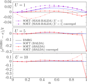
Figure 3: Similar to Fig. 2 but deviations from the DMRG result are plotted (instead of total per-site energies) for ease of comparison. Dashed lines are used for SOET results obtained with self-consistently converged densities.

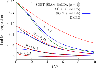
Figure 4: Double occupations plotted as a function of $U/t$ for various exact densities $n=N/L$ with $L=32$. Results obtained with SIAM-BALDA[$n$=1], which is only defined at half-filling, are plotted for $n=1$ (green curve). iBALDA double occupations obtained with self-consistently converged densities (not shown) are almost indistinguishable from the ones obtained with the exact densities. Note that, for $n=1$, the BALDA curve is on top of the DMRG curve, as expected.

As expected, both per-site energies and double occupations are significantly improved when applying the SIAM-BALDA[$n$=1] functional (see Figs. 2 and 4). Let us stress that, in order to obtain similar results in DMET, one would need to increase the number of impurity sites Knizia and Chan (2012) while, at the SIAM-BALDA[$n$=1] level of approximation, we keep on using a single impurity site.

Away from half-filling, SOFT (BALDA) systematically underestimates the double occupation in the weakly-correlated regime, as shown in Fig. 4. This is a direct consequence of the unphysical linear behavior in $U$ of $e^{\rm BA}_{\rm c}(n)$ when $U\rightarrow 0$ and $n\neq 1$ [see Eq. (II.3.1)]. On the other hand, the iBALDA, which uses the “bare” double occupation of the embedded impurity [see Eqs. (21) and (34)] recovers the exact double occupation in the weakly correlated limit ($U=0$) and gives relatively accurate results otherwise. Note that exact densities have been used so far. By solving Eq. (II.1) self-consistently within the iBALDA, we introduce density-driven errors in the per-site energy (see the dashed lines in Fig. 3). In the weakly correlated regime, they are clearly related to the unphysical linearity in $U$ of the BALDA correlation potential [see Eq. (32)]. Note that, at the iBALDA level of approximation, the double occupations obtained self-consistently (not shown) are essentially on top of the ones obtained with the exact densities, simply because the density-functional contribution is neglected. Let us finally mention that, in the vicinity of the half-filled strongly-correlated regime, the iBALDA per-site energy deteriorates if self-consistently converged densities are used (see Fig. 2). As shown in Fig. 5 (see the $U=5$ and $U=10$ panels), the BALDA per-site correlation energy differs substantially from the exact impurity correlation one, especially around $n=1$, thus making the iBALDA approximation irrelevant in this regime of correlation and density. SIAM-BALDA gives, on the other hand, a far more accurate description of the impurity correlation energy than BALDA around half-filling, as illustrated in Fig. 5. Note that, at low density, SIAM-BALDA does not give very accurate impurity correlation energies for large $U$ values, thus somehow invalidating our assumption (see Sec. II.4) that, at low densities, combining Yamada’s expansion in $U/\Gamma$ of the SIAM correlation energy with the density-dependent impurity level width parameter $\Gamma(t,n)$ of Eq. (55) would be sufficient. A better approximation is clearly needed in this regime of correlation and density.

Let us now briefly discuss the performance of SIAM-BALDA. We only show results obtained with the relatively small $U=1$ value for which, at half-filling, Yamada’s perturbation expansion of the SIAM correlation energy is accurate. Although, as discussed previously, SIAM-BALDA provides an overall better description of the density-functional impurity correlation energy than BALDA, even in stronger correlation regimes, its combination with BALDA (see Eq. (56)) for the calculation of per-site energies and double occupations will not necessarily provide good results as $U/t$ increases. Indeed, as readily seen in Eqs. (21) and (23), it is in principle important to reproduce the proper dependence in $t$ and $U$ of the complementary per-site bath correlation functional. Moreover, the density dependence of the SIAM-BALDA impurity correlation energy is far from satisfactory (see Fig. 5), which may lead to substantial density-driven errors. The performance of SIAM-BALDA in stronger correlation regimes will be discussed further in a forthcoming paper. Obviously, the same criticism would apply to the interpolation in Eq. (II.3.2) where the density-dependent $\Gamma(t,n)$ of Eq. (55) could be used for any density $n$ (not just $n=1$). Such a choice would be pragmatic since the interpolation is only justified in the half-filled case. A density-dependent generalization of the interpolation formula would be needed in order to obtain a density-functional approximation that is applicable to any density and correlation regime. Let us finally point out that the use of a density-dependent impurity level width parameter $\Gamma(t,n)$ in the strongly correlated limit of the SIAM correlation functional $E^{\rm SIAM}_{{\rm c},U/\Gamma\rightarrow\infty}(U,\Gamma,n)$ might enhance the density dependence of the embedding potential. It is unclear how physical (or unphysical) this can be. This should obviously be analyzed in detail. We keep such an analysis for future work.

Returning to SIAM-BALDA, it gives, for $U=1$, relatively accurate per-site energies (see Fig. 2). Interestingly, even though density-driven errors are still present, they are substantially reduced when comparison is made with iBALDA, especially in the low density regime (see the dashed lines in the top panel of Fig. 3). This is simply due to the fact that, within SIAM-BALDA, the embedding potential equals the BALDA correlation potential on all sites (bath and impurity) and it is complemented by Yamada’s correlation potential (with a minus sign) on the impurity site only [see Eqs. (37) and (55)]. Since the latter potential is quadratic in $U$, there will be no spurious Hartree contribution to the potential, in contrast to BALDA (as seen from the top panel of Fig. 5), and therefore no self-consistency errors, at least at low density. We also see from Fig. 5 that, when the density increases, the SIAM-BALDA impurity correlation potential, i.e., the derivative of the SIAM-BALDA impurity correlation energy with respect to $n$, is underestimated (in absolute value) which could explain why, in this regime, SIAM-BALDA still induces density-driven errors. We should finally stress that the latter errors might be enhanced by the fact that we use a complementary per-site correlation functional for the bath that depends only on the occupation of the impurity (see Eq. (25)). Double occupations are plotted with respect to the exact density for $U=1$ in Fig. 6. As expected, SIAM-BALDA improves on iBALDA results close to the half-filled case. However, at low density, the SIAM-BALDA per-site correlation for the bath inherits the unphysical linear behavior in $U$ of BALDA (which is removed in iBALDA by construction), thus leading to underestimated double occupations. In summary, the simple version of SIAM-BALDA that we propose is relatively accurate close to half-filling. By construction, it is in principle only applicable to relatively weak correlation regimes. Its generalization to stronger correlation regimes as well as the possibility to include occupations of the bath sites in the design of impurity correlation functionals will be investigated in the future.

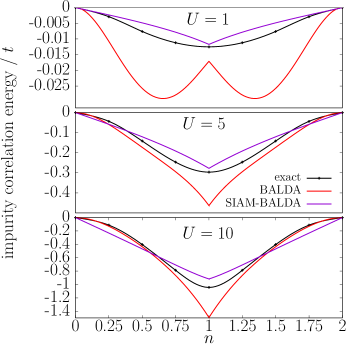
Figure 5: Comparing the density-functional impurity correlation energy used in SIAM-BALDA [see Eqs. (37) and (55)] with the exact results of Ref. Senjean et al. (2017). The latter were obtained for a 8-site ring. The (total) BALDA per-site correlation energy is shown for analysis purposes.

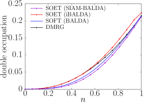
Figure 6: Double occupations plotted as a function of the exact density $n=N/L$ for $U=t=1$ and $L=32$. For iBALDA and SIAM-BALDA, results obtained with self-consistently converged densities (not shown) are almost on top of the ones obtained with the exact densities.

V Conclusions and perspectives

SOET is an in-principle-exact DFT-based embedding theory where the (not necessarily uniform) fully-interacting Hubbard system is mapped onto an impurity-interacting one. In this work, SOET has been applied to the uniform one-dimensional Hubbard model for the purpose of deriving local density approximations. Exact properties of the embedding functionals have been derived first. In particular, we have shown that, in order to calculate per-site energies and double occupations, the contribution of the bath to the per-site correlation energy is, in addition to the latter, the key quantity to model in SOET. Various density-functional approximations, which are based on Bethe ansatz and perturbative solutions to the Hubbard and Anderson models, have been constructed and tested. Each functional is well adapted to a particular regime of correlation and density. For example, one of them (SIAM-BALDA), while performing well around half-filling and in not too strong correlation regimes, inherits the limitations of BALDA away from half-filling. We hope that this work will pave the way to the design of better SOET density functionals that are applicable to all regimes.

Another key aspect of SOET is the self-consistent calculation of the embedded impurity system’s wavefunction. DMRG has been used for that purpose in this work but any other wavefunction-based method could in principle be used in this context. In contrast to the DMET, SOET can easily incorporate correlation effects in the bath thanks to a dedicated density functional. Note that, for practical purposes, the SOET could be reformulated as an open impurity site problem, thus allowing for clearer connections between the two approaches. Work is currently in progress in this direction.

Let us also mention that the impurity problem in SOET could alternatively be solved with a SIAM solver. The use of Green function techniques in SOET is interesting, not only for practical purposes, but also for the development of better density-functional embedding potentials. For that purpose, one would have to derive a Sham–Schlüter equation Sham and Schlüter (1983) for the embedded impurity system. Moreover, a Green-function-based formulation of SOET might provide a convenient framework for comparing SOET with DMFT, in the spirit of Ref. Ayral et al. (2017). Extensions to higher-dimensional  Ijäs and Harju (2010); Karlsson et al. (2011); Capelle and Campo Jr. (2013) and ab-initio Hamiltonians [using localized orbitals or (delocalized) natural molecular orbitals] are also under investigation.

Appendix A Exact expression for the double occupation

In this section, the proof for the SOET-based double occupation expression in Eq. (21) is given. Let us start with Eq. (20) which is valid for a uniform $N$-electron and $L$-site model with density $\underline{n}\equiv\{n_{i}=n\}_{i}$ where $n=N/L$. According to Eq. (18), the double occupation now reads:

$$d = \dfrac{n^{2}}{4}+\dfrac{\partial E_{\rm c}^{\rm imp}(\underline{n})}{\partial U}+\dfrac{\partial\overline{e}_{\rm c}^{\rm bath}(\underline{n})}{\partial U}$$ (57)

$$= \dfrac{\partial E_{\rm Hxc}^{\rm imp}(\underline{n})}{\partial U}+\dfrac{\partial\overline{e}_{\rm c}^{\rm bath}(\underline{n})}{\partial U}.$$

We will come back to this expression later on. Let us now consider the impurity-interacting LL functional in Eq. (10) which is defined for any (i.e., not necessarily uniform) density $\mathbf{n}$. The minimizing wavefunction in Eq. (10), whose density equals $\mathbf{n}$, is denoted $\Psi^{\rm imp}(\mathbf{n})$ so that

$$F^{\rm imp}(\mathbf{n})=\langle\Psi^{\rm imp}(\mathbf{n})|\hat{T}+U\hat{n}_{0\uparrow}\hat{n}_{0\downarrow}|\Psi^{\rm imp}(\mathbf{n})\rangle.$$ (58)

An equivalent and useful expression is obtained from the following Legendre-Fenchel transform Fromager (2015); Senjean et al. (2017):

$$F^{\rm imp}(\mathbf{n})=\sup_{\mathbf{v}}\left\{\mathcal{E}^{\rm imp}(U,t,\mathbf{v})-(\mathbf{v}|\mathbf{n})\right\},$$ (59)

where $\mathcal{E}^{\rm imp}(U,t,\mathbf{v})$ is the ground-state energy of $\hat{H}^{\rm imp}(U,t,\mathbf{v})=\hat{T}+\hat{U}_{0}+\sum_{i}v_{i}\hat{n}_{i}$. Differentiating Eq. (59) with respect to $U$ gives

$$\dfrac{\partial F^{\rm imp}(\mathbf{n})}{\partial U}=\left.\dfrac{\partial\mathcal{E}^{\rm imp}(U,t,\mathbf{v})}{\partial U}\right|_{\mathbf{v}=\mathbf{v}^{\rm emb}(U,t,\mathbf{n})},$$ (60)

where $\mathbf{v}^{\rm emb}(U,t,\mathbf{n})$ is the maximizing (and therefore stationary) potential in Eq. (59), thus leading to the following expression, according to the Hellmann-Feynman theorem,

$$\dfrac{\partial F^{\rm imp}(\mathbf{n})}{\partial U} = \langle\Psi^{\rm imp}(\mathbf{n})|\hat{n}_{0\uparrow}\hat{n}_{0\downarrow}|\Psi^{\rm imp}(\mathbf{n})\rangle$$ (61)

$$= d^{\rm imp}(\mathbf{n}),$$

where we used the fact that $\Psi^{\rm imp}(\mathbf{n})$, whose double occupation for the impurity site is denoted $d^{\rm imp}(\mathbf{n})$, is the ground-state wavefunction of $\hat{H}^{\rm imp}(U,t,\mathbf{v}^{\rm emb}(U,t,\mathbf{n}))$ Fromager (2015); Senjean et al. (2017). Finally, since the non-interacting kinetic energy $T_{\rm s}(\mathbf{n})$ does not depend on $U$, we obtain from Eqs. (13) and (61) the general expression

$$d^{\rm imp}(\mathbf{n})=\dfrac{\partial E^{\rm imp}_{\rm Hxc}(\mathbf{n})}{\partial U}.$$ (62)

Returning to the particular case of a uniform $\mathbf{n}=\underline{n}$ density [see Eq. (57)], it comes from Eq. (62) the following exact expression for the true physical double occupation,

$$d = d^{\rm imp}(\underline{n})+\dfrac{\partial\overline{e}_{\rm c}^{\rm bath}(\underline{n})}{\partial U},$$ (63)

which is equivalent to Eq. (21), since, in the exact theory, the self-consistent solution $\Psi^{\rm imp}$ to Eq. (II.1) equals (in the uniform case) $\Psi^{\rm imp}(\underline{n})$ and $\underline{n}=\mathbf{n}^{\Psi^{\rm imp}(\underline{n})}$.

Appendix B Exact expression for the per-site energy

In this section, the proof for the SOET per-site energy expression in Eq. (23) is given. Let us start with Eq. (22) which is valid for a uniform density profile $\underline{n}$. According to Eq. (18), the per-site energy now reads:

$$e = t_{\rm s}(n)+\dfrac{U}{4}n^{2}+E_{\rm c}^{\rm imp}(\underline{n})+\overline{e}_{\rm c}^{\rm bath}(\underline{n})$$ (64)

$$= t_{\rm s}(n)+E_{\rm Hxc}^{\rm imp}(\underline{n})+\overline{e}_{\rm c}^{\rm bath}(\underline{n}),$$

or, equivalently, according to Eq. (13),

$$e = t_{\rm s}(n)+F^{\rm imp}(\underline{n})-T_{\rm s}(\underline{n})+\overline{e}^{\rm bath}_{\rm c}(\underline{n}).$$ (65)

We will come back to this relation later on. Let us now focus on the impurity-interacting LL functional that, for any (i.e., not necessarily uniform) density $\mathbf{n}$, we decompose into kinetic and interaction energy contributions,

$$F^{\rm imp}(\mathbf{n}) = \langle\Psi^{\rm imp}(\mathbf{n})|\hat{T}+\hat{U}_{0}|\Psi^{\rm imp}(\mathbf{n})\rangle$$ (66)

$$= T^{\rm imp}(\mathbf{n})+U^{\rm imp}(\mathbf{n}),$$

where

$$T^{\rm imp}(\mathbf{n})=\langle\Psi^{\rm imp}(\mathbf{n})|\hat{T}|\Psi^{\rm imp}(\mathbf{n})\rangle,$$ (67)

and

$$U^{\rm imp}(\mathbf{n}) = \langle\Psi^{\rm imp}(\mathbf{n})|\hat{U}_{0}|\Psi^{\rm imp}(\mathbf{n})\rangle$$ (68)

$$= U\langle\Psi^{\rm imp}(\mathbf{n})|\hat{n}_{0\uparrow}\hat{n}_{0\downarrow}|\Psi^{\rm imp}(\mathbf{n})\rangle$$

$$= Ud^{\rm imp}(\mathbf{n}).$$

Following the same strategy as in Eqs. (60) and (61), we obtain

$$\dfrac{\partial F^{\rm imp}(\mathbf{n})}{\partial t} = \left.\dfrac{\partial\mathcal{E}^{\rm imp}(U,t,\mathbf{v})}{\partial t}\right|_{\mathbf{v}=\mathbf{v}^{\rm emb}(U,t,\mathbf{n})}$$ (69)

$$= \dfrac{T^{\rm imp}(\mathbf{n})}{t},$$

which gives, when $U=0$,

$$\dfrac{\partial T_{\rm s}(\mathbf{n})}{\partial t}=\dfrac{T_{\rm s}(\mathbf{n})}{t}.$$ (70)

Combining Eqs. (13), (14), (69) and (70) finally leads to

$$T^{\rm imp}(\mathbf{n}) = t\dfrac{\partial F^{\rm imp}(\mathbf{n})}{\partial t}$$ (71)

$$= T_{\rm s}(\mathbf{n})+t\dfrac{\partial E_{\rm c}^{\rm imp}(\mathbf{n})}{\partial t}.$$

Returning to the uniform case $\mathbf{n}=\underline{n}$, it comes from Eqs. (65), (66), (68), and (71) the following exact expression for the per-site energy,

$$e = t_{\rm s}(n)+Ud^{\rm imp}(\underline{n})+t\dfrac{\partial E_{\rm c}^{\rm imp}(\underline{n})}{\partial t}+\overline{e}_{\rm c}^{\rm bath}(\underline{n}),$$ (72)

which, with the decomposition in Eq. (18) and the fact that $\Psi^{\rm imp}(\underline{n})=\Psi^{\rm imp}$, leads to Eq. (23).

Appendix C Invariance of $\overline{e}_{\rm c}^{\rm bath}(\mathbf{n})$ under hole-particle symmetry and consequences for the embedding potential

Let us consider any density $\mathbf{n}\equiv\{n_{i}\}_{i}$ summing up to a number $N=\sum_{i}n_{i}$ of electrons. Under hole-particle symmetry, this density becomes $(\underline{2}-\mathbf{n})\equiv\{2-n_{i}\}_{i}$ and the number of electrons equals $2L-N$ where $L$ is the number of sites. We will prove that these two densities give the same correlation energy for the impurity. Let us start with the Legendre–Fenchel transform in Eq. (59) [the $t$- and $U$-dependence of the impurity system’s energy is dropped for convenience] which, under hole-particle symmetry, becomes

$$F^{\rm imp}(\underline{2}-\mathbf{n})=\underset{\mathbf{v}}{\rm sup}\Big{\{} \mathcal{E}^{{\rm imp},2L-N}(\mathbf{v})-2\sum_{i}v_{i}$$ (73)

$$+(\mathbf{v}|\mathbf{n})\Big{\}}.$$

From the substitution

$$\mathbf{v}\rightarrow-\mathbf{v},$$ (74)

we obtain the following equivalent expression,

$$F^{\rm imp}(\underline{2}-\mathbf{n})=\underset{\mathbf{v}}{\rm sup}\Big{\{} \mathcal{E}^{{\rm imp},2L-N}(-\mathbf{v})+2\sum_{i}v_{i}-(\mathbf{v}|\mathbf{n})\Big{\}},$$

where $\mathcal{E}^{{\rm imp},2L-N}(-\mathbf{v})$ is the $(2L-N)$-electron ground-state energy of the impurity-interacting Hamiltonian

$$\hat{H}^{\rm imp}(-\mathbf{v}) = -t\sum_{i\sigma}\left(\hat{c}_{i\sigma}^{\dagger}\hat{c}_{i+1\sigma}+\mathrm{H.c.}\right)-\sum_{i\sigma}v_{i}\hat{c}_{i\sigma}^{\dagger}\hat{c}_{i\sigma}$$ (76)

$$+U\hat{c}_{0\uparrow}^{\dagger}\hat{c}_{0\uparrow}\hat{c}_{0\downarrow}^{\dagger}\hat{c}_{0\downarrow}.$$

If we now apply the hole-particle transformation to the creation and annihilation operators,

$$\hat{c}_{i\sigma}^{\dagger} \rightarrow \hat{b}_{i\sigma}^{\dagger}=(-1)^{i}\hat{c}_{i\sigma},$$

$$\hat{c}_{i\sigma} \rightarrow \hat{b}_{i\sigma}=(-1)^{i}\hat{c}_{i\sigma}^{\dagger},$$ (77)

the Hamiltonian in Eq. (76) becomes

$$\hat{H}^{\rm imp}(-\mathbf{v}) = \hat{H}_{h}^{\rm imp}(\mathbf{v})-2\sum_{i}v_{i}$$ (78)

$$+U\left(1-\sum_{\sigma}\hat{b}_{0\sigma}^{\dagger}\hat{b}_{0\sigma}\right),$$

where the hole analog of the impurity-interacting Hamiltonian with arbitrary potential $\mathbf{v}$ reads

$$\hat{H}_{h}^{\rm imp}(\mathbf{v}) = -t\sum_{i\sigma}\left(\hat{b}_{i\sigma}^{\dagger}\hat{b}_{i+1\sigma}+\mathrm{H.c.}\right)+\sum_{i\sigma}v_{i}\hat{b}_{i\sigma}^{\dagger}\hat{b}_{i\sigma}$$ (79)

$$+U\hat{b}_{0\uparrow}^{\dagger}\hat{b}_{0\uparrow}\hat{b}_{0\downarrow}^{\dagger}\hat{b}_{0\downarrow}.$$

By shifting the potential on the impurity site as follows,

$$\mathbf{v}\rightarrow\tilde{\mathbf{v}}\equiv\{v_{i}-U\delta_{i0}\}_{i},$$ (80)

we finally obtain

$$\hat{H}^{\rm imp}(-\mathbf{v}) = \hat{H}_{h}^{\rm imp}(\tilde{\mathbf{v}})-2\sum_{i}v_{i}+U.$$ (81)

As readily seen from Eq. (81), $\hat{H}^{\rm imp}(-\mathbf{v})$ and $\hat{H}_{h}^{\rm imp}(\tilde{\mathbf{v}})$ share the same $(2L-N)$-electron ground state. Moreover, it is clear from Eqs. (76) and (79) that the $(2L-N)$-electron [i.e., $N$-hole] ground-state energy of $\hat{H}_{h}^{\rm imp}(\tilde{\mathbf{v}})$ is nothing but the $N$-electron ground-state energy $\mathcal{E}^{{\rm imp},N}(\tilde{\mathbf{v}})$ of $\hat{H}^{\rm imp}(\tilde{\mathbf{v}})$. From these observations and Eq. (81) we conclude that

$$\mathcal{E}^{{\rm imp},2L-N}(-\mathbf{v}) = \mathcal{E}^{{\rm imp},N}(\tilde{\mathbf{v}})-2\sum_{i}v_{i}+U.$$ (82)

Introducing Eq. (82) into Eq. (C) leads to

$$F^{\rm imp}(\underline{2}-\mathbf{n}) = \underset{\mathbf{v}}{\rm sup}\left\{\mathcal{E}^{{\rm imp},N}(\tilde{\mathbf{v}})-(\mathbf{v}|\mathbf{n})\right\}+U$$ (83)

$$= \underset{\tilde{\mathbf{v}}}{\rm sup}\left\{\mathcal{E}^{{\rm imp},N}(\tilde{\mathbf{v}})-(\tilde{\mathbf{v}}|\mathbf{n})\right\}+U(1-n_{0})$$

$$= F^{{\rm imp}}(\mathbf{n})+U(1-n_{0}).$$

In the particular case $U=0$, we recover the hole-particle symmetry relation for the non-interacting kinetic energy,

$$T_{\rm s}(\underline{2}-\mathbf{n})=T_{\rm s}(\mathbf{n}).$$ (84)

We conclude from Eqs. (83), (84), (13) and (14) that the impurity correlation density-functional energy is invariant under hole-particle symmetry,

$$E_{\rm c}^{\rm imp}(\underline{2}-\mathbf{n})=E_{\rm c}^{\rm imp}(\mathbf{n}).$$ (85)

Since the per-site correlation energy in the uniform system is also invariant Capelle and Campo Jr. (2013),

$$e_{\rm c}(2-n)=e_{\rm c}(n),$$ (86)

it comes from Eq. (18) that $\overline{e}_{\rm c}^{\rm bath}(\mathbf{n})$ is invariant under hole-particle symmetry. As a result, we have

$$-\left.\dfrac{\partial e_{\rm c}(\nu)}{\partial\nu}\right|_{\nu=2-n}=\frac{\partial e_{\rm c}(n)}{\partial n},$$ (87)

and

$$-\left.\dfrac{\partial\overline{e}_{\rm c}^{\rm bath}({\bm{\nu}})}{\partial\nu_{i}}\right|_{{\bm{\nu}}=\underline{2}-\mathbf{n}}=\dfrac{\partial\overline{e}_{\rm c}^{\rm bath}(\bf{n})}{\partial n_{i}},$$ (88)

which, for a half-filled finite-size system gives

$$\left.\frac{\partial e_{\rm c}(n)}{\partial n}\right|_{n=1}=0=\left.\dfrac{\partial\overline{e}_{\rm c}^{\rm bath}(\bf{n})}{\partial n_{i}}\right|_{{\bf n}=\underline{1}}.$$ (89)

Note that, for a finite $L$ value, uniform densities will have discrete values which explains why we do not distinguish ${\bf{n}}\rightarrow\underline{1}^{+}$ and ${\bf{n}}\rightarrow\underline{1}^{-}$ limits and just consider ${\bf{n}}=\underline{1}$. However, in the thermodynamic limit ($L\rightarrow+\infty$), this distinction should be made otherwise the physical band gap cannot be reproduced Lima et al. (2002). Note also that, for a finite-size system with uniform (discrete) density profiles ${\bf n}=\underline{n}$, the maximizing embedding potential in Eq. (73) fulfills, according to Eqs. (74), (C), (80) and (83), the following hole-particle symmetry relation

$${v}_{i}^{\rm emb}(\underline{2}-\underline{n})=-{v}^{\rm emb}_{i}(\underline{n})-U\delta_{i0},$$ (90)

thus leading to, at half-filling,

$${v}^{\rm emb}_{i}(\underline{1})=-\dfrac{U}{2}\delta_{i0}.$$ (91)

The latter result is also recovered from Eq. (89) and Eq. (24).

Appendix D Derivative discontinuity in KS SOFT and SOET at $n=1$ in the atomic limit

Let us consider the fully-interacting $L$-site Hubbard Hamiltonian in the atomic limit ($t=0$),

$$\hat{H}(n)=\hat{U}+v(n)\sum_{i}\hat{n}_{i},$$ (92)

which reproduces the uniform density profile with density $n$. Starting from the half-filling situation ($L$ electrons or, equivalently, $n=1$), we can add an electron in order to investigate the behavior of $v(n)$ when $n\rightarrow 1^{+}$. In order to have a total number of electrons varying continuously from $L$ to $L+1$ or, equivalently, $1<n<(L+1)/L$, the $L$- and $(L+1)$-electron ground states of $\hat{H}(n)$ must be degenerate, thus leading to the following condition,

$$Lv(n)=(L+1)v(n)+U,$$ (93)

or, equivalently, $v(n)=-U$. Therefore we conclude that, in the thermodynamic limit ($L\rightarrow+\infty$),

$$\left.v(n)\right|_{n=1^{+}}=-U.$$ (94)

On the other hand, if we consider the removal of an electron, the density can vary continuously in the range $(L-1)/L<n<1$ if the $(L-1)$- and $L$-electron ground states of $\hat{H}(n)$ are degenerate, thus leading to the condition $(L-1)v(n)=Lv(n)$ and, consequently,

$$\left.v(n)\right|_{n=1^{-}}=0.$$ (95)

Turning to the KS Hamiltonian with ground-state uniform density $n$ (and $t=0$),

$$\hat{H}^{\rm KS}(n)=v^{\rm KS}(n)\sum_{i}\hat{n}_{i},$$ (96)

we can show similarly that, in contrast to the interacting case, the KS potential has no discontinuity at $n=1$,

$$\left.v^{\rm KS}(n)\right|_{n=1^{+}}=\left.v^{\rm KS}(n)\right|_{n=1^{-}}=0.$$ (97)

Consequently, we recover the well-known discontinuous behavior of the correlation potential at half-filling:

$$\left.\dfrac{\partial e_{\rm c}(n)}{\partial n}\right|_{n=1^{+}} = \left.\left(v^{\rm KS}(n)-v(n)-\dfrac{U}{2}n\right)\right|_{n=1^{+}}$$ (98)

$$= +U/2,$$

and

$$\left.\dfrac{\partial e_{\rm c}(n)}{\partial n}\right|_{n=1^{-}} = \left.\left(v^{\rm KS}(n)-v(n)-\dfrac{U}{2}n\right)\right|_{n=1^{-}}$$ (99)

$$= -U/2.$$

Let us now consider the impurity-interacting Hamiltonian of SOET in the atomic limit,

$$\hat{H}^{\rm imp}(n)=\hat{U}_{0}+\sum_{i}v^{\rm emb}_{i}({n})\hat{n}_{i}.$$ (100)

A uniform density $n=(L+1)/L$ is obtained from the $(L+1)$-electron ground state of $\hat{H}^{\rm imp}(n)$ if, for any bath site label $i$ ($i\neq 0$),

$$U+2v^{\rm emb}_{0}(n)+\sum_{k\neq 0}v^{\rm emb}_{k}(n)=2v^{\rm emb}_{i}(n)+\sum_{k\neq i}v^{\rm emb}_{k}(n).$$

The latter degeneracy condition simply ensures that the added electron can occupy either the impurity site or a bath site. In order to let $n$ vary continuously in the range $1<n<(L+1)/L$ we also need the $L$- and $(L+1)$-electron ground states to be degenerate:

$$2v^{\rm emb}_{i}(n)+\sum_{k\neq i}v^{\rm emb}_{k}(n)=\sum_{k}v^{\rm emb}_{k}(n),$$ (102)

thus leading to $v^{\rm emb}_{i}(n)=0$ in the bath and, according to Eq. (D), $v^{\rm emb}_{0}(n)=-U$. If, on the other hand, the density varies in the range $(L-1)/L<n<1$, the degeneracy condition between $(L-1)$- and $L$-electron ground states reads

$$\sum_{k\neq j}v^{\rm emb}_{k}(n)=\sum_{k}v^{\rm emb}_{k}(n).$$ (103)

Note that the latter condition, which leads to $v^{\rm emb}_{j}(n)=0$, holds for any site (impurity or bath) label $j$. In summary, we obtain in the thermodynamic limit,

$$\left.v^{\rm emb}_{0}(n)\right|_{n=1^{-}} = 0,$$

$$\left.v^{\rm emb}_{0}(n)\right|_{n=1^{+}} = -U,$$

$$\left.v^{\rm emb}_{i}(n)\right|_{n=1^{-}} = \left.v^{\rm emb}_{i}(n)\right|_{n=1^{+}}=0,\hskip 5.69046pti\neq 0.$$ (104)

We then conclude from Eqs. (II.1), (15), and (19) that, in the atomic limit, the complementary per-site bath correlation potential exhibits no discontinuous behavior at half-filling, neither on the impurity site,

$$\left.\dfrac{\partial\overline{e}_{\rm c}^{\rm bath}(\mathbf{n})}{\partial n_{0}}\right|_{\mathbf{n}={\underline{1}^{+}}} = \left.\Big{(}v^{\rm emb}_{0}(n)-v(n)\Big{)}\right|_{n=1^{+}}$$ (105)

$$= 0$$

$$= \left.\Big{(}v^{\rm emb}_{0}(n)-v(n)\Big{)}\right|_{n=1^{-}}$$

$$= \left.\dfrac{\partial\overline{e}_{\rm c}^{\rm bath}(\mathbf{n})}{\partial n_{0}}\right|_{\mathbf{n}={\underline{1}^{-}}},$$

nor on the bath sites ($i\neq 0$), since

$$\left.\dfrac{\partial\overline{e}_{\rm c}^{\rm bath}(\mathbf{n})}{\partial n_{i}}\right|_{\mathbf{n}={\underline{1}^{+}}} = \left.\left(v^{\rm emb}_{i}(n)-v(n)-\dfrac{U}{2}n-\dfrac{\partial e_{\rm c}(n)}{\partial n}\right)\right|_{n=1^{+}}$$ (106)

$$= \left.\left(v^{\rm emb}_{i}(n)-v^{\rm KS}(n)\right)\right|_{n=1^{+}}$$

$$= 0$$

$$= \left.\left(v^{\rm emb}_{i}(n)-v^{\rm KS}(n)\right)\right|_{n=1^{-}}$$

$$= \left.\dfrac{\partial\overline{e}_{\rm c}^{\rm bath}(\mathbf{n})}{\partial n_{i}}\right|_{\mathbf{n}={\underline{1}^{-}}}.$$

Note that, as a consequence of Eqs. (98), (99), and (105),

$$\left.\dfrac{\partial E_{\rm c}^{\rm imp}({\bf n})}{\partial n_{0}}\right|_{\mathbf{n}={\underline{1}^{+}}} = \left.\dfrac{\partial e_{\rm c}(n_{0})}{\partial n_{0}}\right|_{n_{0}=1^{+}}-\left.\dfrac{\partial\overline{e}_{\rm c}^{\rm bath}(\mathbf{n})}{\partial n_{0}}\right|_{\mathbf{n}={\underline{1}^{+}}}$$ (107)

$$= +U/2,$$

and

$$\left.\dfrac{\partial E_{\rm c}^{\rm imp}({\bf n})}{\partial n_{0}}\right|_{\mathbf{n}={\underline{1}^{-}}} = \left.\dfrac{\partial e_{\rm c}(n_{0})}{\partial n_{0}}\right|_{n_{0}=1^{-}}-\left.\dfrac{\partial\overline{e}_{\rm c}^{\rm bath}(\mathbf{n})}{\partial n_{0}}\right|_{\mathbf{n}={\underline{1}^{-}}}$$ (108)

$$= -U/2.$$

Therefore, the impurity correlation potential exhibits a discontinuity at half-filling.

References

- Anisimov et al. (1991) V. I. Anisimov, J. Zaanen, and O. K. Andersen, Phys. Rev. B 44, 943 (1991).
- Liechtenstein et al. (1995) A. Liechtenstein, V. Anisimov, and J. Zaanen, Phys. Rev. B 52, R5467 (1995).
- Pulay (1983) P. Pulay, Chem. Phys. Lett. 100, 151 (1983).
- Saebo and Pulay (1993) S. Saebo and P. Pulay, Annu. Rev. Phys. Chem. 44, 213 (1993).
- Hampel and Werner (1996) C. Hampel and H.-J. Werner, J. Chem. Phys. 104, 6286 (1996).
- Sun and Chan (2016) Q. Sun and G. K.-L. Chan, Acc. Chem. Res. 49, 2705 (2016).
- Ayral et al. (2017) T. Ayral, T.-H. Lee, and G. Kotliar, Phys. Rev. B 96, 235139 (2017).
- Georges and Kotliar (1992) A. Georges and G. Kotliar, Phys. Rev. B 45, 6479 (1992).
- Georges et al. (1996) A. Georges, G. Kotliar, W. Krauth, and M. J. Rozenberg, Rev. Mod. Phys. 68 (1996).
- Kotliar and Vollhardt (2004) G. Kotliar and D. Vollhardt, Phys. Today 57, 53 (2004).
- Held (2007) K. Held, Adv. Phys. 56, 829 (2007).
- Zgid and Chan (2011) D. Zgid and G. K.-L. Chan, J. Chem. Phys. 134 (2011).
- Kotliar et al. (2006) G. Kotliar, S. Y. Savrasov, K. Haule, V. S. Oudovenko, O. Parcollet, and C. A. Marianetti, Rev. Mod. Phys. 78, 865 (2006).
- Sun and Kotliar (2002) P. Sun and G. Kotliar, Phys. Rev. B 66, 085120 (2002).
- Biermann et al. (2003) S. Biermann, F. Aryasetiawan, and A. Georges, Phys. Rev. Lett. 90, 086402 (2003).
- Karlsson (2005) K. Karlsson, J. Phys. Condens. Matter 17, 7573 (2005).
- Boehnke et al. (2016) L. Boehnke, F. Nilsson, F. Aryasetiawan, and P. Werner, Phys. Rev. B 94, 201106 (2016).
- Werner and Casula (2016) P. Werner and M. Casula, J. Phys. Condens. Matter 28, 383001 (2016).
- Nilsson et al. (2017) F. Nilsson, L. Boehnke, P. Werner, and F. Aryasetiawan, Phys. Rev. Materials 1, 043803 (2017).
- Kananenka et al. (2015) A. A. Kananenka, E. Gull, and D. Zgid, Phys. Rev. B 91, 121111 (2015).
- Lan et al. (2015) T. N. Lan, A. A. Kananenka, and D. Zgid, J. Chem. Phys. 143, 241102 (2015).
- Lan et al. (2017) T. N. Lan, A. Shee, J. Li, E. Gull, and D. Zgid, Phys. Rev. B 96, 155106 (2017).
- Knizia and Chan (2012) G. Knizia and G. K.-L. Chan, Phys. Rev. Lett. 109, 186404 (2012).
- Knizia and Chan (2013) G. Knizia and G. K.-L. Chan, J. Chem. Theory Comput. 9, 1428 (2013).
- Bulik et al. (2014) I. W. Bulik, G. E. Scuseria, and J. Dukelsky, Phys. Rev. B 89, 035140 (2014).
- Zheng and Chan (2016) B.-X. Zheng and G. K.-L. Chan, Phys. Rev. B 93, 035126 (2016).
- Wouters et al. (2016a) S. Wouters, C. A. Jiménez-Hoyos, Q. Sun, and G. K.-L. Chan, J. Chem. Theory Comput. (2016a).
- Wouters et al. (2016b) S. Wouters, C. A. Jiménez-Hoyos, and G. K.-L. Chan, arXiv preprint arXiv:1605.05547 (2016b).
- Rubin (2016) N. C. Rubin, arXiv preprint arXiv:1610.06910 (2016).
- Tsuchimochi et al. (2015) T. Tsuchimochi, M. Welborn, and T. Van Voorhis, J. Chem. Phys. 143, 024107 (2015).
- Welborn et al. (2016) M. Welborn, T. Tsuchimochi, and T. Van Voorhis, J. Chem. Phys. 145, 074102 (2016).
- Chayes et al. (1985) J. Chayes, L. Chayes, and M. B. Ruskai, J. Stat. Phys. 38, 497 (1985).
- Gunnarsson and Schönhammer (1986) O. Gunnarsson and K. Schönhammer, Phys. Rev. Lett. 56, 1968 (1986).
- Schönhammer et al. (1995) K. Schönhammer, O. Gunnarsson, and R. Noack, Phys. Rev. B 52, 2504 (1995).
- Capelle and Campo Jr. (2013) K. Capelle and V. L. Campo Jr., Phys. Rep. 528, 91 (2013).
- Lima et al. (2002) N. Lima, L. Oliveira, and K. Capelle, Europhys. Lett. 60, 601 (2002).
- Lima et al. (2003) N. A. Lima, M. F. Silva, L. N. Oliveira, and K. Capelle, Phys. Rev. Lett. 90, 146402 (2003).
- Capelle et al. (2003) K. Capelle, N. Lima, M. Silva, and L. Oliveira, in The Fundamentals of Electron Density, Density Matrix and Density Functional Theory in Atoms, Molecules and the Solid State (Springer, 2003), p. 145.
- Franca et al. (2012) V. V. Franca, D. Vieira, and K. Capelle, New J. Phys. 14, 073021 (2012).
- Xianlong et al. (2006) G. Xianlong, M. Polini, M. Tosi, V. L. Campo Jr, K. Capelle, and M. Rigol, Phys. Rev. B 73, 165120 (2006).
- Xianlong et al. (2007) G. Xianlong, M. Rizzi, M. Polini, R. Fazio, M. P. Tosi, V. L. Campo Jr, and K. Capelle, Phys. Rev. Lett. 98, 030404 (2007).
- Silva et al. (2005) M. Silva, N. Lima, A. L. Malvezzi, and K. Capelle, Phys. Rev. B 71, 125130 (2005).
- Akande and Sanvito (2010) A. Akande and S. Sanvito, Phys. Rev. B 82, 245114 (2010).
- Campo Jr and Capelle (2005) V. Campo Jr and K. Capelle, Phys. Rev. A 72, 061602 (2005).
- Xianlong (2008) G. Xianlong, Phys. Rev. B 78, 085108 (2008).
- Bergfield et al. (2012) J. P. Bergfield, Z.-F. Liu, K. Burke, and C. A. Stafford, Phys. Rev. Lett. 108, 066801 (2012).
- Liu et al. (2012) Z.-F. Liu, J. P. Bergfield, K. Burke, and C. A. Stafford, Phys. Rev. B 85, 155117 (2012).
- Liu and Burke (2015) Z.-F. Liu and K. Burke, Phys. Rev. B 91, 245158 (2015).
- Verdozzi (2008) C. Verdozzi, Phys. Rev. Lett. 101, 166401 (2008).
- Kurth et al. (2010) S. Kurth, G. Stefanucci, E. Khosravi, C. Verdozzi, and E. Gross, Phys. Rev. Lett. 104, 236801 (2010).
- Karlsson et al. (2011) D. Karlsson, A. Privitera, and C. Verdozzi, Phys. Rev. Lett. 106, 116401 (2011).
- Stefanucci and Kurth (2011) G. Stefanucci and S. Kurth, Phys. Rev. Lett. 107, 216401 (2011).
- Xianlong et al. (2012) G. Xianlong, A.-H. Chen, I. Tokatly, and S. Kurth, Phys. Rev. B 86, 235139 (2012).
- Schindlmayr and Godby (1995) A. Schindlmayr and R. Godby, Phys. Rev. B 51, 10427 (1995).
- López-Sandoval and Pastor (2002) R. López-Sandoval and G. Pastor, Phys. Rev. B 66, 155118 (2002).
- López-Sandoval and Pastor (2004) R. López-Sandoval and G. Pastor, Phys. Rev. B 69, 085101 (2004).
- Saubanère and Pastor (2009) M. Saubanère and G. Pastor, Phys. Rev. B 79, 235101 (2009).
- Saubanère and Pastor (2011) M. Saubanère and G. Pastor, Phys. Rev. B 84, 035111 (2011).
- Töws and Pastor (2011) W. Töws and G. Pastor, Phys. Rev. B 83, 235101 (2011).
- Töws et al. (2014) W. Töws, M. Saubanère, and G. Pastor, Theor. Chem. Acc. 133, 1 (2014).
- Saubanère et al. (2016) M. Saubanère, M. B. Lepetit, and G. Pastor, Phys. Rev. B 94, 045102 (2016).
- Stefanucci and Kurth (2015) G. Stefanucci and S. Kurth, Nano Lett. 15, 8020 (2015).
- Kurth and Stefanucci (2016) S. Kurth and G. Stefanucci, Phys. Rev. B 94, 241103 (2016).
- Fromager (2015) E. Fromager, Mol. Phys. 113, 419 (2015).
- Senjean et al. (2017) B. Senjean, M. Tsuchiizu, V. Robert, and E. Fromager, Mol. Phys. 115, 48 (2017).
- White (1992) S. R. White, Phys. Rev. Lett. 69, 2863 (1992).
- White (1993) S. R. White, Phys. Rev. B 48, 10345 (1993).
- Verstraete et al. (2008) F. Verstraete, V. Murg, and J. I. Cirac, Adv. Phys. 57, 143 (2008).
- Schollwöck (2011) U. Schollwöck, Ann. Phys. 326, 96 (2011).
- (70) N. Nakatani, [Online]. https://github.com/naokin/mpsxx.
- Lieb and Wu (1968) E. H. Lieb and F. Y. Wu, Phys. Rev. Lett. 20, 1445 (1968).
- Anderson (1961) P. W. Anderson, Phys. Rev. 124, 1 (1961).
- Ying et al. (2014) Z.-J. Ying, V. Brosco, and J. Lorenzana, Phys. Rev. B 89, 205130 (2014).
- Georges (2016) A. Georges, C. R. Phys. 17, 430 (2016).
- Yamada (1975) K. Yamada, Prog. Theo. Phys. 53, 970 (1975).
- Sham and Schlüter (1983) L. J. Sham and M. Schlüter, Phys. Rev. B 51, 1888 (1983).
- Ijäs and Harju (2010) M. Ijäs and A. Harju, Phys. Rev. B 82, 235111 (2010).