Improved robust model selection methods for a Lévy nonparametric regression in continuous time ††thanks: This work was supported by the RSF grant 17-11-01049 (National Research Tomsk State University).
Abstract
In this paper we develop the James - Stein improved method for the estimation problem of a nonparametric periodic function observed with Lévy noises in continuous time. An adaptive model selection procedure based on the weighted improved least squares estimates is constructed. The improvement effect for nonparametric models is studied. It turns out that in non-asymptotic setting the accuracy improvement for nonparametric models is more important, than for parametric ones. Moreover, sharp oracle inequalities for the robust risks have been shown and the adaptive efficiency property for the proposed procedures has been established. The numerical simulations are given.
Key words: Improved non-asymptotic estimation, James - Stein procedures,
Robust quadratic risk, Nonparametric regression, Lévy process,
Model selection, Sharp oracle inequality, Adaptive estimation, Asymptotic efficiency.
AMS (2010) Subject Classification : primary 62G08; secondary 62G05
1 Introduction
Consider the following nonparametric regression model in continuous time
| (1.1) |
where is an unknown - periodic function, is an unobserved noise. The problem is to estimate the function on the observations . Note that, if is a Brownian motion, then we obtain the well-known ”signal+white noise” model which is very popular in statistical radio-physics (see, for example, [15, 25, 26, 34]). In this paper we assume that in addition to intrinsic noises in radio-electronic systems, approximated usually by the gaussian white or color noise, the useful signal is distorted by the impulse flow described by Lévy processes defined in the next section. The cause of a pulse stream can be, for example, either external unintended (atmospheric) or intentional impulse noises or errors in the demodulation and the channel decoding for binary information symbols. Note that, for the first time the impulse noises for the detection signal problems have been studied by Kassam in [18] through compound Poisson processes. Later, such processes was used in [10, 22, 23, 24, 33] for parametric and nonparametric signal estimation problems. It should be noted that such models are too limited, since the compound Poisson process can describe only the large impulses influence with a single fixed frequency. However, the real technical (for example, telecommunication or navigation) systems work under noise impulses having different sizes and different frequencies (see, for example, [35]). To take this into account one needs to use many (may be infinite number) different compound Poisson processes in the same observation model. This is possible to do only in a framework of Lévy processes which are natural extensions for the compound Poisson processes. Moreover, it should be noted also that Lévy models are fruitfully used in the different applied problems (see, for example, [2, 5, 6, 7] and the references therein). In this paper we consider the adaptive estimation problem for the function i.e. when its regularity properties are unknown. To do this we use the model selection methods. The interest to such statistical procedures is explained by the fact that they provide adaptive solutions for the nonparametric estimation through oracle inequalities which give non-asymptotic upper bounds for the quadratic risks including the minimal risk over chosen the estimators family. It will be noted that for the first time the model selection methods were proposed by Akaike [1] and Mallows [28] for parametric models. Then, these methods have been developed for nonparametric estimation problems by Barron, Birgé and Massart [3] and Fourdrinier and Pergamenshchikov [9] for regression models in discrete time and Konev and Pergamenshchikov [21] in continuous time. Unfortunately, the oracle inequalities obtained in these papers can not provide the efficient estimation in the adaptive setting, since the upper bounds in these inequalities have some fixed coefficients in the main terms which are more than one. To obtain the efficiency property one has to obtain the sharp oracle inequalities, i.e. the inequalities in which the coefficient at the principal term is close to unity. To obtain such inequalities for general non-Gaussian observations one needs to use the method proposed by Konev and Pergamenshchikov in [19, 20, 22, 23] for semimartingale models in continuous time based on the model selection tool developed by Galtchouk and Pergamenshchikov in [12, 13] for heteroscedastic non-Gaussian regression models in discrete time.
The goal of this paper is to develop a new sharp model selection method for estimating the unknown signal using the improved estimation approach. Usually, the model selection procedures are based on the least squares estimates. This paper proposes the improved least squares estimates which enable us to improve considerably the non-asymptotic estimation accuracy. For the first time such idea was proposed by Fourdrinier and Pergamenshchikov in [9] for regression models in discrete time and by Konev and Pergamenshchikov in [21] for Gaussian regression models in continuous time. We develop these methods for the non-Gaussian regression models in continuous time. It should be noted that generally for the conditionally Gaussian regression models we can not use the well-known improved estimators proposed in [8, 17] for Gaussian or spherically symmetric observations. To apply the improved estimation methods to the non-Gaussian regression models in continuous time one needs to use the modifications of the well-known James - Stein estimators proposed in [24, 33] for parametric problems. We use these estimators to construct model selection procedures for nonparametric models. Then to study the non-asymptotic accuracy we develop a special analytical tool for the Lévy regression models to obtain sharp oracle inequalities for the improved model selection procedures. Then to study the efficiency property for the proposed estimation procedure we need to obtain a lower bound for the quadratic risks. Usually, to do this one uses the van Trees inequality. In this paper we show the corresponding van Trees inequality for the Lévy regression models and then we derive the needed asymptotic sharp lower bound for the normalized risks, i.e. we find the Pinsker constant for the model (1.1). As to the upper bound, similarly to [20], we use the obtained sharp oracle inequality for the weighted least squares estimators containing the efficient Pinsker procedure. Therefore, through the oracle inequality we estimate from above the risk of the proposed procedure by the risk of the efficient Pinsker procedure up to some coefficient which goes to one. As a result we show the asymptotic efficiency without using the smoothness information of the function .
The rest of the paper is organized as follows. In Section 2 we describe the noise processes in (1.1) and define the main risks for the estimation problem. In Section 3 we construct the improved least squares estimates and study the improvement effect for the Lévy model. In Section 4 we construct the improved model selection procedure and show the sharp oracle inequalities. In Section 5 the Monte Carlo simulation results are given. The asymptotic efficiency is studied in Section 6. In Section 7 we study some properties of the stochastic integrals with respect to the Lévy processes. In Section 8 we prove the van Trees inequality for the model (1.1). In Section 9 we prove all main results and in Appendix we give some technical results.
2 Noise process model
First, we assume that the noise process in (1.1) is defined as
| (2.1) |
where and are some unknown constants, is a standard Brownian motion, ”” denotes the stochastic integral with respect to the compensated jump measure with deterministic compensator , i.e.
Here is a Lévy measure, i.e. some positive measure on , (see, for example, [7, 16] for details) such that
| (2.2) |
We use the notation . Note that the Lévy measure may be equal to . It should be noted that in all papers on the nonparametric signal estimation in the model (1.1) the main condition on the jumps is the finiteness of the Lévy measure, i.e. .
The process (2.1) allows us to consider the several independent impulse noise sources with the different frequencies. Indeed, in this case (see, for example, page 135 in [7]) we introduce compound Poisson processes into the model (1.1) as
| (2.3) |
where are independent Poisson processes with the intensities and the sizes of impulses are independent i.i.d. sequences with and . In this case the Lévy measure for any Borel set is defined as
Next, note, that if
| (2.4) |
then we can introduce the infinite number of the noise jumps setting
| (2.5) |
Moreover, if the total noise intensity , then , i.e. we obtain the observation model with saturated impulse noise.
In the sequel we will denote by the distribution of the process in the Skorokhod space and by we denote all these distributions for which the parameters and satisfy the conditions
| (2.6) |
where the bounds and are functions of , i.e. and such that for any
| (2.7) |
We also assume that the distribution of the noise process is unknown. We know only that this distribution belongs to the distribution family defined in (2.6)–(2.7). By these reasons we use the robust estimation approach developed for nonparametric problems in [11, 22, 23]. To this end we will measure the estimation quality by the robust risk defined as
| (2.8) |
where is an estimate, i.e. any function of , is the usual quadratic risk defined as
| (2.9) |
The first goal in this paper is to develop shrinkage nonparametric estimation methods for which improve the non asymptotic robust estimation accuracy (2.8) with respect to the well known least squares estimators. The next goal is to provide non asymptotic optimality in the sense of sharp oracle inequalities. Moreover, asymptotically, as , our goal is to show the efficiency property for the proposed shrinkage estimators for the risks (2.8).
3 Improved estimation
Let be an orthonormal basis in . We extend these functions by the periodic way on , i.e. = for any .
) Assume that the basis functions are uniformly bounded, i.e. for some , which in general case may be depend on ,
| (3.1) |
For example, we can take the trigonometric basis defined as and for
| (3.2) |
where denotes integer part of .
For estimating the unknown function in (1.1) we consider it’s Fourier expansion
The corresponding Fourier coefficients
can be estimated as
In view of (1.1), we obtain
| (3.3) |
where
As in [20] we define a class of weighted least squares estimates for
| (3.4) |
where the weights belong to some finite set from for which we set
| (3.5) |
where is the number of the vectors in and . In the sequel we assume that all vectors from satisfies the following condition.
Assume that for any vector there exists some fixed integer such that their first components equal to one, i.e. for for any .
Remark 3.1.
Note that the weight coefficients satisfying the condition was introduced in [32] to construct the efficient estimation for the nonparametric regression model in discrete time.
Now we need the - field generated by the jumps of the process (2.1), i.e. we set . To construct the improved estimators we need the following proposition.
Proposition 3.1.
For any the random vector is the - conditionally Gaussian in with zero mean and the covariance matrix
such that
| (3.6) |
where is the maximal eigenvalue of the matrix .
Now, for the first Fourier coefficients in (3.3) we use the improved estimation method proposed for parametric models in [33]. To this end we set . In the sequel we will use the norm for any vector from . Now we define the shrinkage estimators as
| (3.7) |
where
and the threshold is given in the lower bound (3.6). The positive parameter is such that
| (3.8) |
for any .
Now we introduce a class of shrinkage weighted least squares estimates for as
| (3.9) |
We denote the difference of quadratic risks of the estimates (3.4) and (3.9) as
We obtain the following result.
Remark 3.2.
The inequality (3.10) means that non-asymptotically, i.e. for non large , the estimate (3.9) outperforms in mean square accuracy the estimate (3.4). As we will see later in the efficient weight coefficients as for some . Therefore, in view of the definition of the constant in (3.7) and the conditions (2.7) and (3.8) as . This means that improvement is considerably may better than for the parametric regression when the parameter dimension is fixed [33].
4 Model selection
In this section we construct a model selection procedure for the estimation of in (1.1) on the basis of the weighted shrinkage estimators (3.9). To this end we consider the empirical squared error defined as
In order to obtain a good estimate, we have to write a rule to choose a weight vector in (3.9). It is obvious, that the best way is to minimise the empirical squared error with respect to . Making use the estimate definition (3.9) and the Fourier transformation of implies
| (4.1) |
Since the Fourier coefficients are unknown, the weight coefficients can not be found by minimizing this quantity. To circumvent this difficulty one needs to replace the terms by their estimators defined as
| (4.2) |
where is the estimate for the limiting variance of which we choose in the following form
| (4.3) |
For this change in the empirical squared error, one has to pay some penalty. Thus, one comes to the cost function of the form
| (4.4) |
where is some positive constant, is the penalty term defined as
| (4.5) |
We define the improved model selection procedure as
| (4.6) |
It will be noted that exists because is a finite set. If the minimizing sequence in (4.6) is not unique, one can take any minimizer. Now, to write the oracle inequality we set
| (4.7) |
where . It is useful to note that in view of the first condition in (2.7) and the properties (3.8) the constant is not large as , i.e. for any
| (4.8) |
First we study the non asymptotic properties for the procedure (4.6).
Theorem 4.1.
In the case, when the value of is known, one can take and
| (4.10) |
then we can rewrite the oracle inequality (4.9) in the following form
Also we study the accuracy properties for the estimator (4.3).
Proposition 4.2.
Let in the model (1.1) the function is continuously differentiable. Then, there exists some constant such that for any and
| (4.11) |
where is the derivative of the function .
Remark 4.1.
It should be noted that to estimate the parameter in (4.2) we use the equality (3.3) for the Fourier coefficients with respect to the trigonometric basis (3.2), since, as is shown in Lemma A.6 in [19] for any continuously differentiable function and for any the sum can be estimated from above in an explicite form. Therefore, through the trigonometric basis we can estimate the variance uniformly over the functions , when we will study the efficiency property for the proposed procedures.
To obtain the oracle inequality for the robust risk we impose the following additional conditions.
Assume that the upper bound for the basic function defined in (3.1) is such that for any
Assume that the set is such that for any
| (4.12) |
Theorem 4.3.
Remark 4.2.
Note that sharp oracle inequalities similar to (4.9) and (4.13) was obtained earlier by Konev and Pergamenshchikov in [19, 22, 23] for model selection procedures based on the weighted least squares estimates (3.4). Unfortunately, we can not use such oracle inequalities for the model selection procedures, based on the weighted shrinkage estimates (3.9) since they depend non linearly on the coefficients . This is main technical difficulty which doesn’t allow us to use the obtained oracle inequalities. Moreover, in all these papers the oracle inequalities are obtained under condition that the Lévy measure is finite. The inequalities (4.9) and (4.13) are obtained without conditions on the impulse noises.
Now we specify the weight coefficients in the way proposed in [12] for a heteroscedastic regression model in discrete time. Consider a numerical grid of the form
where and . Both parameters and are the functions of such that for any
| (4.14) |
One can take, for example,
For each we introduce the weight sequence as
| (4.15) |
where ,
We set
| (4.16) |
It will be noted that in this case . Therefore, the conditions (4.14) imply the first limit equality in (4.12). Moreover, in view of the definition (4.15) and taking into account that for the function defined in (3.5) can be estimated for any as
Therefore, using here the conditions (2.7) and (4.14) we get the last limit in (4.12), i.e. the condition holds for the set defined in (4.16).
Remark 4.3.
It will be observed that the specific form of weights (4.15) was proposed by Pinsker [34] for the filtration problem with known smoothness of the regression function observed with an additive gaussian white noise in continuous time. Nussbaum [32] used such weights for the gaussian regression estimation problem in discrete time.
5 Monte Carlo simulations
In this section we give the results of numerical simulations to assess the performance and improvement of the proposed model selection procedure (4.6). We simulate the model (1.1) with -periodic function of the form
| (5.1) |
on and the Lévy noise process is defined as
Here is a compound Poisson process with intensity and a Gaussian sequence (see, for example, [23]).
We use the model selection procedure (4.6) with the weights (4.15) in which , , , and . We define the empirical risk as
where the observation frequency and the expectations was taken as an average over replications.
| 100 | 200 | 500 | 1000 | |
|---|---|---|---|---|
| 0.0118 | 0.0089 | 0.0031 | 0.0009 | |
| 0.0509 | 0.0203 | 0.0103 | 0.0064 | |
| 4.3 | 2.3 | 3.3 | 7.1 |
| 100 | 200 | 500 | 1000 | |
|---|---|---|---|---|
| 0.0237 | 0.0103 | 0.0041 | 0.0011 | |
| 0.0509 | 0.0203 | 0.0103 | 0.0064 | |
| 2.1 | 2.2 | 2.5 | 5.8 |
Table 1 gives the values for the sample risks of the improved estimate (4.6) and the model selection procedure based on the weighted LSE (3.15) from [22] for different numbers of observation period . Table 2 gives the values for the sample risks of the the model selection procedure based on the weighted LSE (3.15) from [22] and it’s improved version for different numbers of observation period .
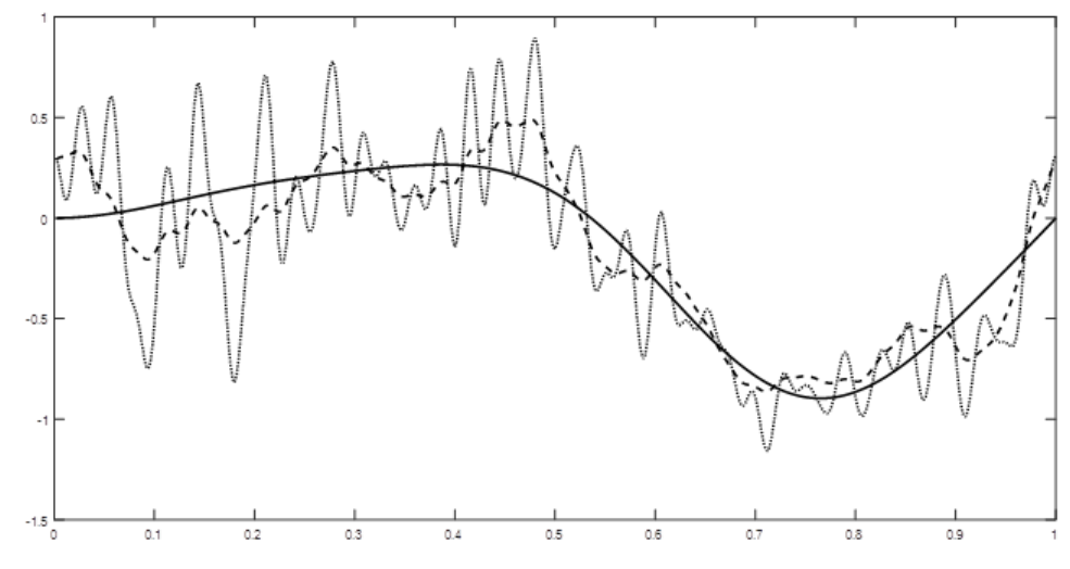
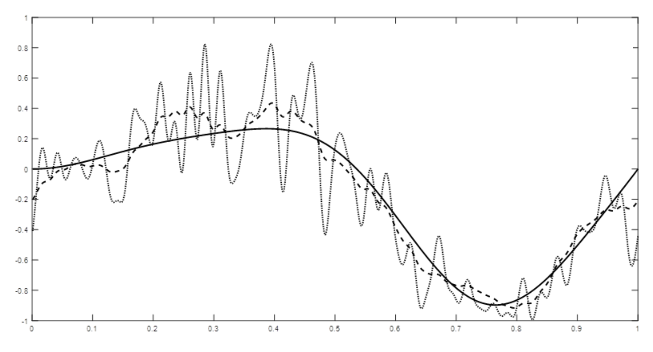
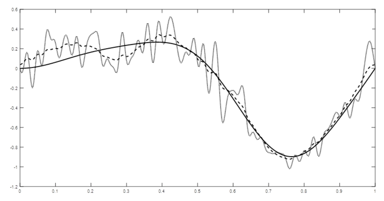
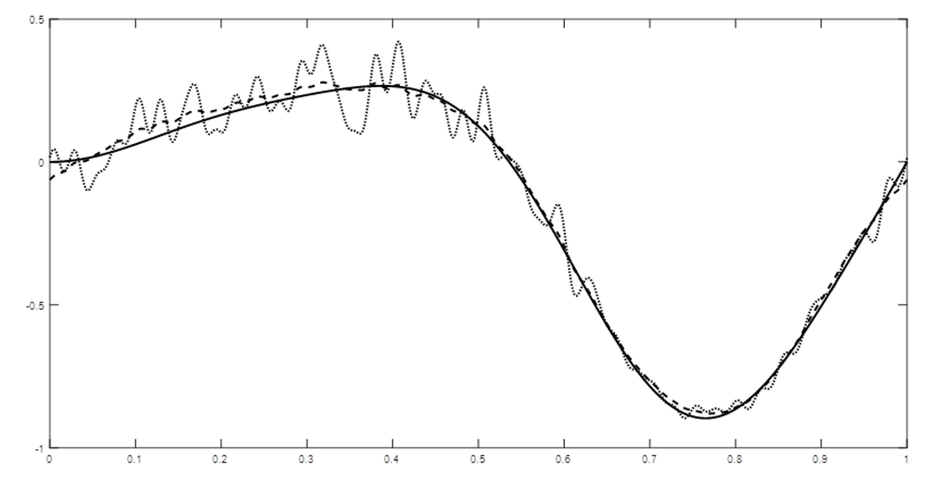
Remark 5.1.
Figures 1–4 show the behavior of the procedures (3.4) and (4.6) depending on the values of observation periods . The bold line is the function (5.1), the continuous line is the model selection procedure based on the least squares estimators and the dashed line is the improved model selection procedure . From the Table 2 for the same with various observations numbers we can conclude that theoretical result on the improvement effect (3.10) is confirmed by the numerical simulations. Moreover, for the proposed shrinkage procedure, Table 1 and Figures 1–4, we can conclude that the benefit is considerable for non large .
6 Asymptotic efficiency
In order to study the asymptotic efficiency we define the following functional Sobolev ball
where and are some unknown parameters, is the space of times differentiable - periodic functions such that for any
In order to formulate our asymptotic results we define the Pinsker constant which gives the lower bound for normalized asymptotic risks
| (6.1) |
It is well known that for any the optimal rate of convergence is (see, for example, [34, 32]). On the basis of the model selection procedure we construct the adaptive procedure for which we obtain the following asymptotic upper bound for the quadratic risk, i.e. we show that the parameter (6.1) gives a lower bound for the asymptotic normalized risks. To this end we denote by the set of all estimators of measurable with respect to the process (1.1), i.e. measurable with respect to -field .
Theorem 6.1.
The robust risk (2.8) admits the following asymptotic lower bound
We show that this lower bound is sharp in the following sense.
Theorem 6.2.
The quadratic risk (2.8) for the estimating procedure has the following asymptotic upper bound
Corollary 6.3.
The model selection procedure is asymptotically efficient, i.e.
| (6.2) |
Remark 6.1.
Remark 6.2.
It should be noted that the equality (6.2) means that the robust efficiency holds with the convergence rate
It is well known that for the simple risks the optimal (minimax) estimation convergence rate for the functions from the set is (see, for example, [34, 32, 15]). So, if the distribution upper bound as we obtain the more rapid rate, and if as we obtain the more slow rate. In the case when is constant the robust rate is the same as the classical non robust convergence rate.
Remark 6.3.
The property (6.2) means that the model selection procedure (4.6) asymptotically has the same efficiency property as the LSE model selection (see, [13, 20]). So, it means that the proposed shrinkage method non-asymptotically has benefit with respect to LSE and asymptotically the shrinkage methods keep the efficiency property.
7 Stochastic calculus for the Lévy processes
In this section we study the process (2.1). First we recall the Novikov inequalities, [31], also referred to as the Bichteler–Jacod inequalities, see [4, 30], providing bounds of the moments of the supremum of purely discontinuous local martingales for and for any
| (7.1) |
where is some positive constant. Further for any two functions and from with we use the following notations
| (7.2) |
Proposition 7.1.
Now we set
| (7.4) |
For any function we introduce the following uniform norm
Proposition 7.2.
Let and be two borel functions such that and . Then for any
| (7.5) |
Proof. Using (A.2) with we can obtain that the process satisfies the following stochastic equation
Note that from the definition of in (A.2) we can represent as
| (7.6) |
where and
Moreover, by the Ito formula
where . Using the last in condition (2.2) and the inequality (7.1) we can obtain that for any bounded measurable function
| (7.7) |
From this and the Hölder inequality we obtain that
Therefore, in view of Proposition (7.1)
From the definition of the discrete part of in (7.6) we can represent the jumps term as
| (7.8) |
where ,
and . In view of Proposition 7.1 and the upper bound (7.7) and taking into account that we calculate
Similarly, we obtain that
and . So,
and, therefore,
Taking into account here that and the conditions of the proposition we obtain the upper bound (7.5). Hence Proposition 7.2. ∎
Now for any we define the following function
| (7.9) |
For this we show the following property.
Proposition 7.3.
For any
| (7.10) |
8 The van Trees inequality for the Lévy processes
In this section we consider the following continuous time parametric regression model (1.1) with the function defined as
with the unknown parameters . Here we assume that the functions are -periodic and orthogonal functions.
Let us denote by the distribution of the process on the Skorokhod space . From Proposition A.2 it follows that in this space for any parameters , the distribution of the process (1.1) is absolutely continuous with respect to the and the corresponding Radon-Nikodym derivative, for any function from , is defined as
| (8.1) |
where
and for any measurable set in with
Let be a prior density on having the following form:
where is some continuously differentiable density in . Moreover, let be a continuously differentiable function such that, for each ,
| (8.2) |
where . For any -measurable integrable function we denote
where .
Lemma 8.1.
For any -measurable square integrable function and for any , the following inequality holds
where
Proof. First of all note that, the density (8.1) on the process is bounded with respect to and for any
Now, we set
Taking into account the condition (8.2) and integrating by parts yield
Now by the Bouniakovskii-Cauchy-Schwarz inequality we obtain the following lower bound for the quadratic risk
To study the denominator in the left hand of this inequality note that in view of the representation (8.1)
Therefore, for each ,
and
Using equality
we get
Hence Lemma 8.1. ∎
9 Proofs
9.1 Proof of Theorem 3.2
Consider the quadratic error of the estimate (3.9)
where for . Therefore, we can represent the risk for the improved estimate as
where . Now, taking into account that the vector is the conditionally gaussian vector in with mean and covariance matrix , we obtain
Here is the conditional distribution density of the vector , i.e.
Recall, that the denotes the transposition. Changing the variables by , one finds that
where and denotes the -th element of . Furthermore, integrating by parts, the integral can be rewritten as
In view of the inequality and Proposition 3.1 we obtain that
Moreover, using the Jensen inequality we can estimate the last expectation from below as
From Proposition 7.1 and the condition (2.6) we obtain
So, for
and, therefore,
Hence Theorem 3.2. ∎
9.2 Proof of Theorem 4.1
Using the definitions (4.1), (4.2) and (4.4), we obtain that for any
| (9.1) |
Now we set
| (9.2) |
where and . Taking into account the definition (4.5), we can rewrite (9.1) as
| (9.3) |
where the function is defined in (3.5), . Let be a fixed sequence in and be as in (4.6). Substituting and in (9.3), we consider the difference
where and
| (9.4) |
Note that . Moreover, note also that
| (9.5) |
where is defined in (4.7). Therefore, through the Cauchy–Schwarz inequality we can estimate the term as
where for . So, applying the elementary inequality
| (9.6) |
with some arbitrary , we get
Moreover, by the same method we estimate the term , i.e.
where
Note that from Proposition 7.3 we obtain that
| (9.7) |
Using the bounds above, one has
The setting and the estimating where this is possible by in this inequality imply
Moreover, taking into account here that
and that , we obtain that
| (9.8) |
Now we examine the third term in the right-hand side of this inequality. Firstly we note that
| (9.9) |
where and
We remind that the set is defined in (9.4). Using Proposition 7.1 we can obtain that for any fixed
| (9.10) |
and, therefore,
| (9.11) |
Moreover, the norm can be estimated from below as
where . Therefore, in view of (3.3)
where . Note that the first term in this inequality we can estimate as
Note that, similarly to (9.11) we can estimate the last term as
From this it follows that for any
| (9.12) |
Moreover, note now that the property (9.5) yields
| (9.13) |
Taking into account that and using the inequality (9.6), we get that for any
To estimate the last term in the right hand of (9.12) we use first the Cauchy – Schwarz inequality and then the bound (9.13), i.e.
Therefore,
So, using all these bounds in (9.12), we obtain that
Using in the inequality (9.9) this bound and the estimate
we obtain
Choosing here we obtain that
From here and (9.8), it follows that
Choosing here and estimating by where this is possible, we get
Taking the expectation and using the upper bound for in Lemma A.1 with yields
where . The inequality holds for each , this implies Theorem 4.1. ∎
9.3 Proof of Theorem 6.1
Firstly, note, that for any fixed
| (9.14) |
Now for any fixed we set
| (9.15) |
Next we approximate the unknown function by a trigonometric series with terms, i.e. for any array , we set
To define the Bayesian risk we choose a prior distribution on as
where are i.i.d. gaussian random variables and the coefficients
Furthermore, for any function , we denote by its projection in onto , i.e.
Since is a convex set, we obtain
Therefore,
Using the distribution we introduce the following Bayes risk
Taking into account now that we obtain
| (9.16) |
with
Therefore, in view of (9.14)
| (9.17) |
In Lemma A.3 we studied the last term in this inequality. Now it is easy to see that
where So, in view of Lemma 8.1 and reminding that we obtain
Therefore, using now the definition (9.15), Lemma A.3 and the inequality (9.17) we obtain that
Taking here limit as we come to the Theorem 6.1. ∎
9.4 Proof of Theorem 6.2
10 Conclusion
In the conclusion we would like to emphasize that in this paper we develop a new model selection method based on the improved versions of the least squares estimates. It turns out that the improvement effect in the nonparametric estimation given in (3.10) is more important than for the parameter estimation problems since the accuracy improvement is proportional to the parameter dimension which goes to infinity for nonparametric models. Recall that, the improved estimation methods was usually used for the parametric estimation problem only, where the parameter dimension is always fixed (see, for example, [8]). Therefore, the benefit in the non-asymptotic quadratic accuracy from the application of the improved estimation methods is more significant in statistical nonparametric signal processing. Moreover, for the proposed improved model selection procedures we obtain the sharp oracle inequalities. It should be emphasized that in this paper we obtain these inequalities without conditions on the jumps, i.e. without assumption that the Lévy measure is finite. To this end we developed a special analytical tool in Proposition 7.2 to study the non-asymptotic properties for the corresponding stochastic integrals with respect to the process (2.1). Moreover, asymptotically, as goes to infinity, we shown the adaptive efficiency for the improved model selection procedures. This is the meaning, that the proposed shrinkage model selection procedures have the benefit with respect to the least squares estimator in the non-asymptotic accuracy and asymptotically they possess the same efficient properties as the least squares methods. Moreover, the behavior of the constructed procedures is illustrated by the numerical simulations in Section 5.
Acknowledgements. This work was partially supported by the research project no. 2.3208.2017/4.6 (the Ministry of Education and Science of the Russian Federation), RFBR Grant 16-01-00121 A and ”The Tomsk State University competitiveness improvement programme” Grant 8.1.18.2018. The work of the last author was partially supported by the Russian Federal Professor program (project no. 1.472.2016/1.4, the Ministry of Education and Science of the Russian Federation) and by the European research project XterM - Feder, University of Havre (France).
11 Appendix
A.1 Proof of Proposition 3.1
Using (2.1) we put for any square integrated functions
From here and (3.3) we can see that the vector has the conditionally Gaussian distribution with respect to with zero mean and its covariance matrix can be rewritten as
where is the identity matrix and the -th element of the matrix is defined as . Using the celebrated inequality of Lidskii and Wieland (see, for example, in [29], G.3.a., p.334) we obtain
Now, using (2.6) we come to desire results. ∎
A.2 Proof of Proposition 4.2
We use here the same method as in [19]. Using the equality (3.3) for the trigonometric basis, we get
where
Therefore, the estimator (4.3) can be represented as
| (A.1) |
where . Note that for the continuously differentiable functions (see, for example, Lemma A.6 in [19]) the Fourrier coefficients for any satisfy the following inequality
and . The second term in (A.1) can be estimated through the equality (9.10), i.e.
Moreover, taking into account that the expectation we can represent the last term in (A.1) as
where the function is defined in (9.2) for . Therefore, similarly to (9.7) we find
This implies that
and, therefore, we obtain the bound (A.2). Hence Proposition 4.2. ∎
A.3 Proof of Proposition 7.1
Proof. Taking into account the definition of in (3.3) and (2.1) we obtain through the Ito formula that
| (A.2) |
where
and . Using now the inequality (7.1) with and we obtain that for any
Therefore, taking the expectation in (A.2) we obtain (7.3). Hence Proposition 7.1. ∎
A.4 Property of Penalty term
Lemma A.1.
A.5 The absolute continuity of distributions for the Lévy processes
In this section we study the absolute continuity for the the Lévy processes defined as
| (A.4) |
where is any arbitrary nonrandom square integrated function, i.e. from and is the Lévy process of the form (2.1) with nonzero constant . We denote by and the distributions of the processes and on the Skorokhod space . Now for any from we set
| (A.5) |
where is the continuous part of the process defined in (8.1). Now we study the measures and in .
Proposition A.2.
For any the measure in and the Radon-Nikodym derivative is
Proof. Note that to show this proposition it suffices to check that for any any for
taking into account that the processes and have the independent homogeneous increments, to this end one needs to check only that for any and
| (A.6) |
To check this equality note that the process
is the gaussian martingale. From here we directly obtain the squation (A.6). Hence Proposition A.2. ∎
A.6 Properties of the term
Lemma A.3.
For any the term introduced in (9.16) satisfies the following property
| (A.7) |
Proof. First, setting , we obtain that
Moreover, note that one can check directly that
So, for sufficiently large we obtain that
where ,
Through the correlation inequality from [14] we can get that for any there exists some constant for which
i.e. the expectation as . Therefore, using the Chebychev inequality we obtain that for any
Hence Lemma A.3. ∎
References
- [1] Akaike H. A new look at the statistical model identification. IEEE Trans. on Automatic Control 19 (1974) 716–723.
- [2] O. E. Barndorff-Nielsen and N. Shephard. Non-Gaussian Ornstein-Uhlenbeck-based models and some of their uses in financial mathematics. J. Royal Stat. Soc. B 63 (2001) 167–241.
- [3] Barron A., Birgé L. and Massart P. (1999) Risk bounds for model selection via penalization. Probab. Theory Relat. Fields 113, 301–415.
- [4] Bichteler K., Jacod J. Calcul de Malliavin pour les diffusions avec sauts: existence d’une densité dans le cas unidimensionnel. Séminaire de probabilité, XVII, Lecture Notes in Math., 986, Springer, Berlin, 1983, 132–157.
- [5] J. Bertoin. Lévy Processes. Cambridge University Press, Cambridge, 1996.
- [6] Comte, F. and Genon-Catalot, V. (2011) Estimation for Lévy processes from high frequency data within a long time interval. The Annals of Statistics, 39(2), 803 – 837.
- [7] Cont R., Tankov P. Financial Modelling with Jump Processes. Chapman & Hall, 2004.
- [8] Fourdrinier D., Strawderman W. E. (1996). A paradox concerning shrinkage estimators: should a known scale parameter be replaced by an estimated value in the shrinkage factor? Journal of Multivariate Analysis, 59(2), 109 –140.
- [9] Fourdrinier D., Pergamenshchikov S. (2007) Improved selection model method for the regression with dependent noise. Annals of the Institute of Statistical Mathematics, 59(3), 435–464.
- [10] Flaksman, A.G. (2002) Adaptive signal processing in antenna arrays with allowance for the rank of the impule-response matrix of a multipath channel Radiophysics and Quantum Electronics, 45 (12), 977 – 988.
- [11] Galtchouk L.I., Pergamenshchikov S.M. (2006) Asymptotically efficient estimates for nonparametric regression models. Statistics and Probability Letters, 76 (8), 852–860.
- [12] Galtchouk L.I., Pergamenshchikov S. M. (2009) Sharp non-asymptotic oracle inequalities for nonparametric heteroscedastic regression models. Journal of Nonparametric Statistics 21 (1), 1 - 16.
- [13] Galtchouk L., Pergamenshchikov S. (2009) Adaptive asymptotically efficient estimation in heteroscedastic nonparametric regression.Journal of Korean Statistical Society, 38(4), 305–322.
- [14] Galtchouk L., Pergamenshchikov S. (2013) Uniform concentration inequality for ergodic diffusion processes observed at discrete times. Stochastic Processes and their Applications, 123, 91–109
- [15] Ibragimov I. A., Khasminskii R. Z. Statistical Estimation: Asymptotic Theory. Springer, New York, 1981.
- [16] Jacod J., Shiryaev A.N. Limit theorems for stochastic processes. 2nd edition, Springer, Berlin, 2002.
- [17] James W., Stein C. (1961). Estimation with quadratic loss. In Proceedings of the Fourth Berkeley Symposium Mathematics, Statistics and Probability, University of California Press, Berkeley, 1, 361–380
- [18] Kassam S.A. Signal detection in non-Gaussian noise. – New York: Springer-Verlag Inc., IX, 1988.
- [19] Konev V. V., Pergamenshchikov S. M. Nonparametric estimation in a semimartingale regression model. Part 1. Oracle Inequalities. Journal of Mathematics and Mechanics of Tomsk State University 3 (2009) 23–41.
- [20] Konev V. V., Pergamenshchikov S. M. Nonparametric estimation in a semimartingale regression model. Part 2. Robust asymptotic efficiency. Journal of Mathematics and Mechanics of Tomsk State University 4 (2009) 31–45.
- [21] Konev V. V., Pergamenshchikov S. M. General model selection estimation of a periodic regression with a Gaussian noise. Annals of the Institute of Statistical Mathematics 62 (2010) 1083–1111.
- [22] Konev V. V., Pergamenshchikov S. M. Efficient robust nonparametric estimation in a semimartingale regression model. Ann. Inst. Henri Poincaré Probab. Stat., 48 (4), 2012, 1217–1244.
- [23] Konev V. V., Pergamenshchikov S. M. Robust model selection for a semimartingale continuous time regression from discrete data. Stochastic processes and their applications, 125, 2015, 294 – 326.
- [24] Konev V., Pergamenshchikov S. and Pchelintsev E. (2014) Estimation of a regression with the pulse type noise from discrete data. Theory Probab. Appl., 58 (3), 442–457.
- [25] Kutoyants Yu. A. Estimation of the signal parameter in a Gaussian Noise. Problems of Information Transmission, 1977, vol. 13 (4), p. 29 – 36.
- [26] Kutoyants Yu. A. Parameter Estimation for Stochastic Processes. Heldeman-Verlag, Berlin, 1984.
- [27] Jacod J., Shiryaev A. N. Limit theorems for stochastic processes. Vol.1, Springer, New York, 1987.
- [28] Mallows C. Some comments on .Technometrics 15 (1973) 661–675.
- [29] Marshall A.W., Olkin I. Inequalities: Theory of Majorization and Its Applications. Springer Series in Statistics, Springer, Academic.
- [30] Marinelli C., Röckner M. (2014) On maximal inequalities for purely discontinuous martingales in infinite dimensions. Séminaire de Probabilités, Lect. Notes Math., XLVI , 293–315.
- [31] Novikov A.A. (1975) On discontinuous martingales. Theory Probab. Appl., 20, 1, 11–26.
- [32] Nussbaum M. (1985) Spline smoothing in regression models and asymptotic efficiency in .- Ann. Statist. 13, 984–997.
- [33] Pchelintsev E. (2013) Improved estimation in a non-Gaussian parametric regression. Stat. Inference Stoch. Process., 16 (1), 15 – 28.
- [34] Pinsker M.S. (1981) Optimal filtration of square integrable signals in gaussian white noise. Problems of Transimission information 17, 120–133.
- [35] Proakis J. G. Digital Communications. McGraw-Hill, New York, 1995.