Homogenization of a class of one-dimensional nonconvex viscous Hamilton-Jacobi equations with random potential

Abstract.

We prove the homogenization of a class of one-dimensional viscous Hamilton-Jacobi equations with random Hamiltonians that are nonconvex in the gradient variable. Due to the special form of the Hamiltonians, the solutions of these PDEs with linear initial conditions have representations involving exponential expectations of controlled Brownian motion in a random potential. The effective Hamiltonian is the asymptotic rate of growth of these exponential expectations as time goes to infinity and is explicit in terms of the tilted free energy of (uncontrolled) Brownian motion in a random potential. The proof involves large deviations, construction of correctors which lead to exponential martingales, and identification of asymptotically optimal policies.

1. Introduction

1.1. Main results

Let $(\Omega,{\mathcal{F}},\mathbb{P})$ be a probability space and $\{T_{y}:\Omega\to\Omega\}_{y\in\mathbb{R}}$ a group of measure preserving transformations with $T_{0}=\text{Id},\ T_{x+y}=T_{x}T_{y}$. Furthermore, assume that the group action is ergodic, that is every set which is invariant under all $T_{y},\ y\in\mathbb{R}$, has measure $0$ or $1$.

We are interested in the behavior as $\varepsilon\to 0$ of a family of solutions $u^{\varepsilon}(t,x,\omega)$, $\varepsilon>0$, to the Cauchy problem

(1.1) $$\frac{\partial u^{\varepsilon}}{\partial t}=\frac{\varepsilon}{2}\frac{\partial^{2}u^{\varepsilon}}{\partial x^{2}}+H_{\beta,c}\left(\frac{\partial u^{\varepsilon}}{\partial x},T_{x/\varepsilon}\,\omega\right) ,\quad(t,x)\in(0,\infty)\times\mathbb{R},$$

(1.2) $$u^{\varepsilon}\Big{|}_{t=0}=g(x) ,\quad x\in\mathbb{R},$$

where $g$ is in $\text{UC}(\mathbb{R})$, the space of uniformly continuous functions, and the Hamiltonian

$$H_{\beta,c}:\mathbb{R}\times\Omega\to\mathbb{R},\quad H_{\beta,c}(p,\omega)=\frac{1}{2}\,p^{2}-c|p|+\beta V(\omega),$$

depends on two constant parameters $c\geq 0$ and $\beta>0$. An important feature of this Hamiltonian is that for all $\beta,c>0$ it is nonconvex (and not level-set convex) in $p$. The random environment enters $H_{\beta,c}$ and (1.1) through the potential $V\in L^{\infty}(\Omega,{\mathcal{F}},\mathbb{P})$ and its shifts $V(T_{x/\varepsilon}\omega),\ x\in\mathbb{R}$. We shall assume without further loss of generality that

(1.3) $$\mathrm{ess\,inf\,}V(\omega)=0\quad\text{and}\quad\mathrm{ess\,sup\,}V(\omega)=1.$$

The parameter $\beta$ is then just the “magnitude” of the potential. We shall also suppose that $\forall\omega\in\Omega$

(1.4) $$x\mapsto V(T_{x}\omega)\ \text{is in $C_{b}^{1}(\mathbb{R})$}.$$

Here and throughout, $C^{k}$ (resp. $C_{b}^{k}$), $k=1,2$, refers to the set of functions that are $k$ times differentiable with continuous (resp. continuous and uniformly bounded) derivatives up to order $k$ inclusively. The above conditions guarantee that the Cauchy problem (1.1)-(1.2) has a unique viscosity solution in $\text{UC}([0,\infty)\times\mathbb{R})$. See Section 5.1 for references.

To state our last assumption on $V$ we need the following definition.

Definition 1.1.

For any $\omega\in\Omega$ and $h\in(0,1)$, an interval $I$ is said to be an $h$-valley (resp. $h$-hill) if $V(T_{x}\omega)\leq h$ (resp. $V(T_{x}\omega)\geq h$) for every $x\in I$.

We shall assume that for every $h\in(0,1)$ and $y>0$

(1.5) $$\mathbb{P}(\text{$[0,y]$ is an $h$-valley})>0\ \ \text{and}\ \ \mathbb{P}(\text{$[0,y]$ is an $h$-hill})>0.$$

Condition (1.5) ensures (for $\mathbb{P}$-a.e. $\omega$ by the ergodicity assumption) the existence of arbitrarily long intervals where the potential is uniformly close to its “extremes”.

We prove the following homogenization result.

Theorem 1.2.

Assume that $V$ satisfies (1.3), (1.4) and (1.5). For every $\theta\in\mathbb{R}$, let $u^{\varepsilon}_{\theta}$ be the unique viscosity solution of the Cauchy problem (1.1)-(1.2) in $\text{UC}([0,\infty)\times\mathbb{R})$ with $g(x)=\theta x$. Then

$$\mathbb{P}\left(\forall R>0\ \forall T>0\ \lim_{\varepsilon\to 0}\max_{|x|\leq R}\max_{t\leq T}|u^{\varepsilon}_{\theta}(t,x,\omega)-\overline{H}_{\beta,c}(\theta)t-\theta x|=0\right)=1,$$

where a continuous function $\overline{H}_{\beta,c}$, the effective Hamiltonian, is given explicitly in terms of the (non-explicit) tilted free energy of a Brownian motion in the potential $\beta V$ (see (2.1), (4.7) and (4.8)).

Example 1.3.

Let $f\geq 0$ be a $C_{b}^{1}(\mathbb{R})$ function with compact support such that $\int_{-\infty}^{\infty}f(x)dx=1$. Define

$$\omega_{x}=\int_{-\infty}^{\infty}f(x-y)g(L_{y}-L_{y-1})dy$$

where $L$ is a standard two-sided Poisson or Wiener process with $L_{0}=0$ and $g(a)=(a\vee 0)\wedge 1$. Set $\omega=(\omega_{x})_{x\in\mathbb{R}}$ and denote the induced probability space by $(\Omega,\mathcal{F},\mathbb{P})$. Define $T_{x}$ naturally by $(T_{x}\omega)_{y}=\omega_{x+y}$ and let $V(\omega)=\omega_{0}$.

We leave it to the reader to check that Example 1.3 falls within our model and satisfies conditions (1.3)-(1.5). The potential in this example has a finite range of dependence. However, our assumptions in general do not imply that the potential is even weakly mixing. In the discrete setting, this was shown in [YZ17, Example 1.3] and the argument carries over easily to the continuous setting.

Note that the function $\overline{u}_{\theta}(t,x)=\overline{H}_{\beta,c}(\theta)t+\theta x$ satisfies the equation

(1.6) $$\frac{\partial\overline{u}}{\partial t}=\overline{H}_{\beta,c}\left(\frac{\partial\overline{u}}{\partial x}\right),\quad(t,x)\in(0,\infty)\times\mathbb{R},$$

and the initial condition $\overline{u}(0,x)=\theta x$. It is the unique viscosity solution of this Cauchy problem in $\text{UC}([0,\infty)\times\mathbb{R})$, see Section 5.1. Moreover, $\overline{H}_{\beta,c}(\theta)=\overline{u}_{\theta}(1,0)=\lim_{\varepsilon\to 0}u^{\varepsilon}_{\theta}(1,0,\omega)$. Using general results from [DK17] we deduce the following corollary.

Corollary 1.4.

Assume that $V$ satisfies the conditions in Theorem 1.2. For every $g\in\text{UC}(\mathbb{R})$, let $u^{\varepsilon}_{g}(t,x,\omega)$ be the unique viscosity solution of (1.1) in $\text{UC}([0,\infty)\times\mathbb{R})$ with the initial condition $g$. Then

$$\mathbb{P}\left(\forall g\in\text{UC}(\mathbb{R})\ \forall R>0\ \forall T>0\ \lim_{\varepsilon\to 0}\max_{|x|\leq R}\max_{t\leq T}|u^{\varepsilon}_{g}(t,x,\omega)-\overline{u}_{g}(t,x)|=0\right)=1,$$

where $\overline{u}_{g}$ is the unique viscosity solution of (1.6) in $\text{UC}([0,\infty)\times\mathbb{R})$ with the initial condition $g$.

Thus, we obtain a full homogenization result for a new class of viscous Hamilton-Jacobi equations with nonconvex (when $c>0$) Hamiltonians in dimension 1.

The solution of (1.1)-(1.2) rewritten as a terminal value problem is also known to characterize the value of a two-player, zero-sum stochastic differential game (see, for instance, [FS89]). But due to the special form of (1.1), our homogenization problem admits a simple and useful control interpretation, where, roughly speaking, the role of one of the players is implicitly assumed by the diffusion in the random environment. More precisely, let $(X_{t})_{t\geq 0}$ be a standard Brownian motion (BM) that is independent of the environment. We denote by $(\mathcal{G}_{t})_{t\geq 0}$ the natural filtration and by $P_{0}$ (resp. $E_{0}$) the probability (resp. expectation) corresponding to this BM when $X_{0}=0$. By the Hopf-Cole transformation and scaling, i.e., setting $u^{\varepsilon}_{\theta}(t,x,\omega)=\varepsilon\log v_{\theta}(t/\varepsilon,x/\varepsilon,\omega)$, we get that $v_{\theta}(t,x,\omega)$ satisfies the $\varepsilon$-independent equation

$$\frac{\partial v_{\theta}}{\partial t}=\frac{1}{2}\frac{\partial^{2}v_{\theta}}{\partial x^{2}}-c\left|\frac{\partial v_{\theta}}{\partial x}\right|+\beta V(T_{x}\omega)v_{\theta},\quad(t,x)\in(0,\infty)\times\mathbb{R},$$

and the initial condition $v_{\theta}(0,x,\omega)=e^{\theta x}$. Taking for simplicity $t=1$ and $x=0$ and using the control representation for $v_{\theta}$ (see (5.5)-(5.6)), the limiting behavior of $u^{\varepsilon}_{\theta}(1,0,\omega)$ as $\varepsilon\to 0$ boils down to showing the existence of the limit (with $S=1/\varepsilon$)

(1.7) $$\overline{H}_{\beta,c}(\theta)=\lim_{\varepsilon\to 0}u^{\varepsilon}_{\theta}(1,0,\omega)=\lim_{S\to\infty}\inf_{\alpha\in{\mathcal{P}}_{c}}\frac{1}{S}\log E_{0}\left[e^{\beta\int_{0}^{S}V(T_{X^{\alpha}_{s}}\omega)\,ds+\theta X^{\alpha}_{S}}\right],$$

where

$${\mathcal{P}}_{c}=\{\alpha=(\alpha_{s})_{s\geq 0}:\ \alpha\ \text{is $[-c,c]$-valued and $\mathcal{G}_{s}$-progressively measurable}\}$$

is the set of admissible controls, and $(X^{\alpha}_{s})_{s\geq 0}$ is defined by

(1.8) $$X^{\alpha}_{s}=\int_{0}^{s}\alpha_{r}\,dr+X_{s}.$$

The control interpretation (1.7) indicates that, contrary to the case $c=0$ for which the existence of the limit can be easily shown by subadditivity arguments, allowing $c>0$ destroys subadditivity. Hence, even the existence of the limit in (1.7) becomes a nontrivial statement. We are able not only to show that the limit in (1.7) exists and get a semi-explicit expression for it but also to provide asymptotically optimal controls (see Section 4.3).

Recall that the original Hamiltonian $H_{\beta,c}(p,\omega)$ is nonconvex in $p$ for all $\beta,c>0$. We show that in our setting the convexity/nonconvexity of the effective Hamiltonian depends only on the magnitude of the potential and the size of the control. More precisely, $\overline{H}_{\beta,c}$ is convex if and only if $\beta\geq c^{2}/2$ (see Figure 1). The “convexification” of the effective Hamiltonian has been previously observed for the first order Hamilton-Jacobi equations in [ATY15], [ATY16], [QTY17].

1.2. Broader context

We shall refer to the equation of the form

(1.9) $$\frac{\partial u^{\varepsilon}}{\partial t}=\frac{\varepsilon}{2}\text{tr\,}(A(T_{x/\varepsilon}\omega)D^{2}u^{\varepsilon})+H(Du^{\varepsilon},T_{x/\varepsilon}\omega),\quad(t,x)\in(0,\infty)\times\mathbb{R}^{d},$$

as a viscous Hamilton-Jacobi equation if the symmetric positive semi-definite matrix $A\not\equiv 0$ and as an inviscid Hamilton-Jacobi equation (or simply Hamilton-Jacobi equation) if $A\equiv 0$.

By change of variables we can always write $u^{\varepsilon}(t,x,\omega)=\varepsilon u(t/\varepsilon,x/\varepsilon,\omega)$ where $u(t,x,\omega)$ solves (1.9) for $\varepsilon=1$. Thus, we are interested in the existence of a scaling limit under the hyperbolic scaling of time and space. Note that linear initial conditions are invariant under this scaling. We shall say that (1.9) with initial condition $g(x)$ homogenizes if with probability one $u^{\varepsilon}(t,x,\omega)$ converges locally uniformly in $t$ and $x$ to the solution $\overline{u}(t,x)$ of a deterministic PDE with the same initial condition. If the convergence is only in probability then we shall say that the problem homogenizes in probability.

It has been shown that if the Hamiltonian $H(p,\omega)$ is convex in the momentum variables ($p\in\mathbb{R}^{d}$), then homogenization holds for very general viscous and inviscid Hamilton-Jacobi equations in all dimensions. The literature on the subject is vast. We shall focus primarily on the viscous case and refer the reader to [LS05], [KRV06], [AS12], [AT14], [AC15a], and the references therein.

If the Hamiltonian $H(p,x)$ is 1-periodic in each of the spatial variables, then there is a general method of proving homogenization due to [LPV87] (see [Eva92] for an extension to general first and second order fully nonlinear PDEs). The method is based on the construction of correctors. Correctors are sublinear (at infinity) solutions to a certain family of nonlinear eigenvalue problems, see (2.11) for our case. The applicability of the method does not depend on the convexity of the Hamiltonian but rather on the coercivity of the Hamiltonian in $p$ and the compactness of the space ($x$ changes on a torus). The method of correctors originated in the study of linear partial differential equations with periodic coefficients, and we refer the interested reader to the monographs [BLP78], [JKO94].

In the more general stochastic setting, [RT00, Theorem 4.1] asserted that if sublinear correctors exist for each vector in $\mathbb{R}^{d}$ then the (inviscid) stochastic problem homogenizes. However, soon it was shown ([LS03]) that in the stochastic case correctors need not exist in general. Thus, other methods were developed. One of them was introduced already in [LPV87] as an alternative method for the (inviscid) periodic problem with a convex Hamiltonian. Convexity played an important role. First of all, it allowed one to use the control representation of solutions. Furthermore, the convexity assumption implied the subadditivity of certain solution-defining quantities, and the homogenization result could be obtained from a subadditive ergodic theorem.

The first two papers which addressed the stochastic homogenization of viscous Hamilton-Jacobi equations, [LS05] and [KRV06], used variational representations of the solutions. In an attempt to steer away from representation formulas and following some ideas in [Szn94] and [LS10], the paper [AS12] introduced a method based on the so-called metric problem. The convexity assumption gives a subadditivity property to solutions of the metric problem and, thus, still essentially restricts the approach to convex Hamiltonians (level-set convex in the inviscid case, [AS13]). This approach was further developed in [AT14] and [AC15a] where some assumptions are relaxed and a rate of convergence is obtained.

For quite some time it was not clear whether the convexity assumption can be disposed of in the stochastic setting. Several classes of examples of nonconvex Hamiltonians for which homogenization holds were recently constructed: [ATY15], [ATY16], [Gao16], [FS16], [QTY17] for inviscid equations and [AC15b], [DK17] for viscous equations. On the other hand, the work [Zil15] has demonstrated that homogenization could fail for nonconvex Hamiltonians in the general stationary and ergodic setting for dimensions $d\geq 2$. (See also [FS16].) These results indicate that the homogenization or non-homogenization for nonconvex Hamiltonians depends significantly on the interplay between the nonconvexity and the random environment, and that one cannot expect a comprehensive solution. The case of viscous equations is particularly difficult, since the viscosity term adds yet another randomness, encoded in the diffusion. The critical scaling at which the diffusion enters the equation brings into play the large deviations for this diffusion and makes the analysis even more challenging.

In spite of the negative results of [LS03] on the existence of correctors for (1.9), the quest for them has never ended (see, for example, [DS09], [DS12], [AC15b]). In particular, the authors of [CS17] have shown under quite general conditions that if the equation (1.9) homogenizes in probability to an effective equation with some continuous and coercive Hamiltonian $\overline{H}(p)$ then correctors exist for every $p$ that is an extreme point of the convex hull of the sub-level set $\{q\in\mathbb{R}^{d}:\,\overline{H}(q)\leq\overline{H}(p)\}$. In discrete multidimensional settings such as first passage percolation, random walks in random environments and directed polymers, the existence of correctors (and closely related Busemann functions) also received a lot of attention (see, e.g., [Yil11], [DH14], [Kri16], [GRAS16], [BL16]).

1.3. Motivation, method and outline

Given the above developments and the complexity of the general homogenization problem with a nonconvex Hamiltonian, one can start with a more modest goal and look first at some model examples of viscous Hamilton-Jacobi equations in dimension 1. For the inviscid case in dimension 1 there are already quite general homogenization results, see [ATY15] and [Gao16]. It is natural to conjecture that homogenization in dimension 1 holds under general assumptions in the viscous case as well. Methods which were used in the inviscid case are not applicable to the viscous case due to the presence of the diffusion term.

In this paper we provide a new class of examples in the viscous one-dimensional case for which homogenization holds. Our examples, in a way, complement some of those considered earlier in [DK17, Theorem 4.10]. More precisely, the method of [DK17] is applicable to Hamiltonians which have one or more “pinning points” (i.e. values $p^{*}$ such that $H(p^{*},\cdot)\equiv\text{const}$) and are convex in $p$ in between the pinning points. For example, $H(p,\omega)=\frac{1}{2}\,p^{2}-b(\omega)|p|$, $b(\omega)>0$, is pinned at $p^{*}=0$ and is convex in $p$ on $(-\infty,0)$ and $(0,\infty)$. Adding a non-constant potential breaks the pinning property. Currently it is not known if (1.9) with

(1.10) $$H(p,\omega)=\frac{1}{2}\,|p|^{2}-b(\omega)|p|+\beta V(\omega)$$

and $A\equiv\text{const}\not\equiv 0$ homogenizes even in dimension 1. Our results give a positive answer in the case when $b(\omega)\equiv c>0$ and $V$ satisfies (1.3)-(1.5).

To prove Theorem 1.2 we first consider the convex case $c=0$ (no-control case for (1.7)) and construct a function $F_{\beta,\theta}$ for every $\theta$ outside of the closed interval where the tilted free energy $\Lambda_{\beta}(\theta)$ (see (2.1)) attains its minimum value $\beta$, i.e. outside of the so-called “flat piece” of the effective Hamiltonian $\overline{H}_{\beta,0}\equiv\Lambda_{\beta}$. The function $F_{\beta,\theta}$ is used to introduce the exponential martingale $M_{t}(\omega)$, see (2.12); for this reason we call $F_{\beta,\theta}$ a corrector. The martingale $M_{t}(\omega)$ immediately yields the desired limit. For each $c>0$ we build the effective Hamiltonian $\overline{H}_{\beta,c}$ by shifting and bridging together pieces of $\Lambda_{\beta}(\cdot\pm c)$ (see Section 4.3 and Figure 1). We note that in our setting correctors exist for all $\theta$ outside of the “flat pieces” of $\overline{H}_{\beta,c}(\theta)$ and coincide with those constructed in the no-control case for an appropriately shifted $\theta$. We use each of these correctors to define an exponential expression (see (4.4)) which turns out to be (i) a submartingale for arbitrary control policies and (ii) a martingale for specific control policies that we deduce to be asymptotically optimal.

The above approach was first proposed and implemented in [YZ17] in the discrete setting where the BM in the control problem (1.7) is replaced by a random walk, the analog of Theorem 1.2 is proved for a viscous Hamilton-Jacobi partial difference equation and the effective Hamiltonian is shown to have the same structure as in this paper. However, as it is often the case, the arguments in the continuous formulation differ noticeably. We believe that some of the ideas in [YZ17] and this paper can be extended to more general settings, for example, to Hamiltonians of the form (1.10) in one or more dimensions.

We end this introduction with a brief outline of the rest of the paper. Section 2 focuses on the no-control case. We obtain a uniform lower bound using the existence of arbitrarily long high hills, construct the aforementioned correctors, use them to give a self-contained proof of the existence of the tilted free energy (Theorem 2.9) and list some of the properties of the latter (Proposition 2.10). Section 3 contains upper bounds for the control problem. We restrict the infimum in (1.7) to bang-bang policies, consider the constant policies $\overleftarrow{\alpha}\equiv-c$ and $\overrightarrow{\alpha}\equiv c$ as well as a family of policies $\alpha^{(x_{*},h,y)}$ which tries to trap the particle to low valleys. These upper bounds produce the graphs in Figure 1. Section 4 provides matching lower bounds. We obtain a uniform lower bound similar to that in the no-control case, use the correctors outside of the flat pieces as mentioned above, give a scaling argument at the elevated flat piece centered at the origin when $\beta<c^{2}/2$, and thereby prove the existence of the effective Hamiltonian (Theorem 4.3). Finally, Section 5 wraps up the solution of the homogenization problem. We derive the control representation and put our limit results (Theorems 2.9 and 4.3) together with relevant results from [DK17] to prove Theorem 1.2 and Corollary 1.4. Note that the regularity assumption (1.4) on $V$ is used only in Section 5 and it is replaced by the weaker continuity assumption (2.2) in Sections 2, 3 and 4.

2. No control

We start our analysis with the special case of no control, $c=0$, where the limit on the RHS of (1.7) simplifies to

(2.1) $$\overline{H}_{\beta,0}(\theta)=\Lambda_{\beta}(\theta)=\lim_{t\to\infty}\frac{1}{t}\log E_{0}\left[e^{\beta\int_{0}^{t}V(T_{X_{s}}\omega)ds+\theta X_{t}}\right].$$

In this section, we assume that $V$ satisfies (1.3), (1.5) and $\forall\omega\in\Omega$

(2.2) $$x\mapsto V(T_{x}\omega)\ \text{is H\"{o}lder continuous with some positive exponent.}$$

Under these assumptions, we prove that the limit in (2.1) exists for all $\beta>0$, $\theta\in\mathbb{R}$ and $\mathbb{P}$-a.e. $\omega$. To this end, we define

(2.3) $$\Lambda_{\beta}^{L}(\theta) =\liminf_{t\to\infty}\frac{1}{t}\log E_{0}\left[e^{\beta\int_{0}^{t}V(T_{X_{s}}\omega)ds+\theta X_{t}}\right]$$

and

$$\Lambda_{\beta}^{U}(\theta) =\limsup_{t\to\infty}\frac{1}{t}\log E_{0}\left[e^{\beta\int_{0}^{t}V(T_{X_{s}}\omega)ds+\theta X_{t}}\right].$$

The quantity $\Lambda_{\beta}(\theta)$ is referred to as the tilted free energy of BM. Its existence is covered by the works [LS05, KRV06] on the homogenization of viscous Hamilton-Jacobi equations with convex Hamiltonians. We give a short and self-contained proof which relies on the construction of correctors and provides an implicit formula for $\Lambda_{\beta}(\theta)$. Introducing these correctors is in fact our main motivation here since they will play a key role in our solution of the control problem (i.e. showing the existence of the limit on the RHS of (1.7) for $c>0$) in Section 4.

2.1. Uniform lower bound (no control)

Throughout the paper, we make use of the hitting times

$$\tau_{y}=\inf\{t\geq 0:\,X_{t}=y\}\quad\text{and}\quad\tau_{\pm y}=\tau_{-y}\wedge\tau_{y},\quad y\in\mathbb{R}.$$

Lemma 2.1.

For every $y>0$,

$$\lim_{t\to\infty}\frac{1}{t}\log P_{0}(\tau_{\pm y}>t)=-\frac{\pi^{2}}{8y^{2}}.$$

Proof.

This follows immediately from the spectral analysis of the Laplace operator on $[-y,y]$ with Dirichlet boundary conditions (see [Var07, Section 5.8]). ∎

Lemma 2.2.

For every $\beta>0$, $\theta\in\mathbb{R}$ and $\mathbb{P}$-a.e. $\omega$, we have $\Lambda_{\beta}^{L}(\theta)\geq\beta$ with the notation in (2.3).

Proof.

By (1.5) and ergodicity, for every $h\in(0,1)$, $y>0$ and $\mathbb{P}$-a.e. $\omega$, there is an $h$-hill of the form $[x^{*}-y,x^{*}+y]$ for some $x^{*}\in\mathbb{R}$ (which depends on $\omega$). Using the strong Markov property and Lemma 2.1, we get

$$\Lambda_{\beta}^{L}(\theta)\geq\liminf_{t\to\infty}\frac{1}{t}\log E_{0}\left[e^{\beta\int_{0}^{t}V(T_{X_{s}}\omega)ds+\theta X_{t}}{{\rm 1\mkern-1.5mu}\!{\rm I}}_{\{\tau_{x^{*}}\leq 1\}\cap\{|X_{s}-x^{*}|<y\ \text{for every}\ s\in[\tau_{x^{*}},t]\}}\right]\geq\beta h-\frac{\pi^{2}}{8y^{2}}.$$

Finally, we send $h\to 1$ and $y\to\infty$. ∎

2.2. Correctors

For every $\beta>0$, $\lambda\geq\beta$, $\omega\in\Omega$ and $x,y\in\mathbb{R}$, let

$$v_{\beta}^{\lambda}(\omega,x;y)=E_{x}\left[e^{\beta\int_{0}^{\tau_{y}}V(T_{X_{s}}\omega)ds-\lambda\tau_{y}}\right].$$

We make two elementary observations. First,

(2.4) $$v_{\beta}^{\lambda}(\omega,x;z)=v_{\beta}^{\lambda}(\omega,x;y)\,v_{\beta}^{\lambda}(\omega,y;z)$$

by the strong Markov property of BM whenever $x\leq y\leq z$ or $x\geq y\geq z$. Second, since $V(\cdot)\in[0,1]$, it follows from Lemma 2.3 (below) that

(2.5) $$\sqrt{2(\lambda-\beta)}|x-y|\leq-\log v_{\beta}^{\lambda}(\omega,x;y)\leq\sqrt{2\lambda}|x-y|.$$

Lemma 2.3.

For every $a\geq 0$ and $x,y\in\mathbb{R}$,

$$E_{x}\left[e^{-a\tau_{y}}\right]=e^{-\sqrt{2a}|x-y|}.$$

Proof.

See [RY99, Chapter 2, Proposition 3.7]. ∎

For every $\beta>0$, $\theta\neq 0$, $\lambda\geq\beta$, $\omega\in\Omega$ and $x\in\mathbb{R}$, let

(2.6) $$F_{\beta,\theta}^{\lambda}(\omega,x) =\begin{cases}-\log v_{\beta}^{\lambda}(\omega,0;x)-\theta x&\text{if $\theta x\geq 0$,}\\ \quad\log v_{\beta}^{\lambda}(\omega,x;0)-\theta x&\text{if $\theta x<0$.}\end{cases}$$

It follows from (2.4) that

(2.7) $$F_{\beta,\theta}^{\lambda}(\omega,x)=\log v_{\beta}^{\lambda}(\omega,x;z)-\log v_{\beta}^{\lambda}(\omega,0;z)-\theta x$$

for every $z\in\mathbb{R}$ such that $(\theta x)^{+}\leq\theta z$. Using this representation, it is easy to check that

(2.8) $$F_{\beta,\theta}^{\lambda}(\omega,x)+F_{\beta,\theta}^{\lambda}(T_{x}\omega,y)=F_{\beta,\theta}^{\lambda}(\omega,x+y)$$

for every $\omega\in\Omega$ and $x,y\in\mathbb{R}$. We refer to this identity as the cocycle property.

In the following lemma and the rest of the paper, we use the notation $(\cdot)^{\prime}=\frac{\partial}{\partial x}(\cdot)$ and $(\cdot)^{\prime\prime}=\frac{\partial^{2}}{\partial x^{2}}(\cdot)$.

Lemma 2.4.

For every $\beta>0$, $\theta\neq 0$, $\lambda\geq\beta$ and $\omega\in\Omega$, the function $x\mapsto F_{\beta,\theta}^{\lambda}(\omega,x)$ is in $C^{2}(\mathbb{R})$ and

$$\frac{1}{2}\left(F_{\beta,\theta}^{\lambda}\right)^{\prime\prime}+\frac{1}{2}\left(\theta+\left(F_{\beta,\theta}^{\lambda}\right)^{\prime}\right)^{2}+\beta V(T_{x}\omega)=\lambda,\quad x\in\mathbb{R}.$$

Proof.

For every $\beta>0$, $\lambda\geq\beta$, $\omega\in\Omega$ and $y\in\mathbb{R}$, the function $x\mapsto v_{\beta}^{\lambda}(\omega,x;y)$ is in $C^{2}(\mathbb{R}\setminus\{y\})$ and

$$\frac{1}{2}\left(v_{\beta}^{\lambda}\right)^{\prime\prime}(\omega,x;y)+\left(\beta V(T_{x}\omega)-\lambda\right)v_{\beta}^{\lambda}(\omega,x;y)=0,\quad x\in\mathbb{R}\setminus\{y\},$$

by (1.3) and (2.2). See [Dyn02, Chapter 6, Section 3]. The desired result follows from taking the logarithm of $v_{\beta}^{\lambda}$ and using the representation in (2.7). ∎

So far we have been working with an arbitrary $\lambda\geq\beta$. In Lemma 2.6 below, we identify a particular choice of $\lambda$.

Lemma 2.5.

If $\theta>0$ and $\beta\leq\lambda<\Lambda_{\beta}^{U}(\theta)$, then $\mathbb{E}[F_{\beta,\theta}^{\lambda}(\cdot,1)]\leq 0$.

Proof.

For every $t>0$,

$$E_{0}\left[e^{\beta\int_{0}^{t}V(T_{X_{s}}\omega)ds+\theta X_{t}}\right]e^{-t\lambda} =\sum_{k=0}^{\infty}E_{0}\left[e^{\int_{0}^{t}[\beta V(T_{X_{s}}\omega)-\lambda]ds+\theta X_{t}}{{\rm 1\mkern-1.5mu}\!{\rm I}}_{\{\tau_{k}<t\leq\tau_{k+1}\}}\right]$$

$$\leq\sum_{k=0}^{\infty}E_{0}\left[e^{\int_{0}^{t}[\beta V(T_{X_{s}}\omega)-\lambda]ds+\theta(k+1)}{{\rm 1\mkern-1.5mu}\!{\rm I}}_{\{\tau_{k}<t\leq\tau_{k+1}\}}\right]$$

$$\leq\sum_{k=0}^{\infty}e^{\theta}E_{0}\left[e^{\int_{0}^{\tau_{k}}[\beta V(T_{X_{s}}\omega)-\lambda]ds+\theta k}\right]$$

(2.9) $$=\sum_{k=0}^{\infty}e^{\theta}\prod_{j=0}^{k-1}E_{j}\left[e^{\int_{0}^{\tau_{j+1}}[\beta V(T_{X_{s}}\omega)-\lambda]ds}\right]e^{\theta}$$

(2.10) $$=\sum_{k=0}^{\infty}e^{\theta+\sum_{j=0}^{k-1}[\log v_{\beta}^{\lambda}(T_{j}\omega,0;1)+\theta]}=\sum_{k=0}^{\infty}e^{\theta-\sum_{j=0}^{k-1}F_{\beta,\theta}^{\lambda}(T_{j}\omega,1)}.$$

The equality in (2.9) follows from the strong Markov property of BM. We take $\limsup$ as $t\to\infty$, use $\Lambda_{\beta}^{U}(\theta)-\lambda>0$ and deduce that the RHS of (2.10) is infinite. This implies that $\mathbb{E}[F_{\beta,\theta}^{\lambda}(\cdot,1)]\leq 0$, since otherwise the RHS of (2.10) would be finite by the Birkhoff ergodic theorem. ∎

Lemma 2.6.

If $\beta<\Lambda_{\beta}^{U}(\theta)$, then there exists a $\lambda_{o}=\lambda_{o}(\beta,\theta)\geq\Lambda_{\beta}^{U}(\theta)$ such that $\mathbb{E}[F_{\beta,\theta}^{\lambda_{o}}(\cdot,1)]=0$.

Proof.

Assume that $\theta>0$. The map $\lambda\mapsto\mathbb{E}[F_{\beta,\theta}^{\lambda}(\cdot,1)]$ is continuous and strictly increasing for $\lambda\geq\beta$. Moreover,

$$\lim_{\lambda\to\infty}\mathbb{E}\left[F_{\beta,\theta}^{\lambda}(\cdot,1)\right]=\infty.$$

These assertions follow from the $P_{0}$-a.s. positivity of $\tau_{1}$, the uniform (in $\omega$) bounds in (2.5) and the dominated convergence theorem. Recalling Lemma 2.5, we deduce the desired result. The $\theta<0$ case is similar. ∎

In the rest of this paper, we write $F_{\beta,\theta}(\omega,x)=F_{\beta,\theta}^{\lambda_{o}}(\omega,x)$ for notational brevity. We give two lemmas which are elementary but of central importance in our analysis both when $c=0$ and $c>0$.

Lemma 2.7.

Assume that $\beta<\Lambda_{\beta}^{U}(\theta)$. Then, the following bounds hold for every $\omega\in\Omega$ and $x\in\mathbb{R}$.

$$\theta+(F_{\beta,\theta})^{\prime}(\omega,x)\in\begin{cases}[\sqrt{2(\lambda_{o}(\beta,\theta)-\beta)},\sqrt{2\lambda_{o}(\beta,\theta)}]&\text{if $\theta>0$,}\\ [-\sqrt{2\lambda_{o}(\beta,\theta)},-\sqrt{2(\lambda_{o}(\beta,\theta)-\beta)}]&\text{if $\theta<0$.}\end{cases}$$

Proof.

For every $\omega\in\Omega$, $x\in\mathbb{R}$ and $y>0$, we use the cocycle property (2.8) to write

$$\frac{1}{y}\left(F_{\beta,\theta}(\omega,x+y)-F_{\beta,\theta}(\omega,x)\right)=\frac{1}{y}F_{\beta,\theta}(T_{x}\omega,y),$$

recall (2.5)-(2.6), send $y\to 0$ and deduce the desired bounds. ∎

Lemma 2.8.

If $\beta<\Lambda_{\beta}^{U}(\theta)$, then $\sup\{|F_{\beta,\theta}(\omega,x)|:|x|\leq t\}=o(t)$ for $\mathbb{P}$-a.e. $\omega$.

Proof.

For $\mathbb{P}$-a.e. $\omega$, $F_{\beta,\theta}(\omega,x)=o(|x|)$ by Lemma 2.6, the cocycle property (2.8) and the Birkhoff ergodic theorem. Hence, for every $\varepsilon>0$, there exists a $t_{0}=t_{0}(\varepsilon)$ such that $|F_{\beta,\theta}(\omega,x)|\leq\varepsilon|x|$ for $|x|\geq t_{0}$. From this we deduce that

$$t^{-1}\sup\{|F_{\beta,\theta}(\omega,x)|:|x|\leq t\} \leq t^{-1}\sup\{|F_{\beta,\theta}(\omega,x)|:|x|\leq t_{0}\}\vee|x|^{-1}\sup\{|F_{\beta,\theta}(\omega,x)|:|x|\geq t_{0}\}$$

$$\leq t^{-1}\sup\{|F_{\beta,\theta}(\omega,x)|:|x|\leq t_{0}\}\vee\varepsilon\leq\varepsilon$$

for sufficiently large $t>t_{0}$. ∎

To summarize, the function $x\mapsto F_{\beta,\theta}(\omega,x)$ is defined whenever $\beta<\Lambda_{\beta}^{U}(\theta)$ (see Lemma 2.6). For $\mathbb{P}$-a.e. $\omega$, it is a sublinear (at infinity) solution of

(2.11) $$\frac{1}{2}\left(F_{\beta,\theta}\right)^{\prime\prime}+\frac{1}{2}\left(\theta+\left(F_{\beta,\theta}\right)^{\prime}\right)^{2}+\beta V(T_{x}\omega)=\lambda_{o}(\beta,\theta),\quad x\in\mathbb{R},$$

by Lemmas 2.4 and 2.8. We refer to this family of functions as correctors.

2.3. The tilted free energy

For every $t\geq 0$, $\omega\in\Omega$, $\beta>0$ and $\theta\neq 0$ such that $\beta<\Lambda_{\beta}^{U}(\theta)$, let

(2.12) $$M_{t}(\omega)=M_{t}(\omega\,|\,\beta,\theta)=e^{\beta\int_{0}^{t}V(T_{X_{s}}\omega)ds+\theta X_{t}+F_{\beta,\theta}(\omega,X_{t})-\lambda_{o}(\beta,\theta)t}.$$

Observe that $M_{0}(\omega)=e^{\theta x+F_{\beta,\theta}(\omega,x)}$ when $X_{0}=x$. Since

(2.13) $$0<M_{t}(\omega)<e^{\theta X_{t}+F_{\beta,\theta}(\omega,X_{t})}\leq e^{\sqrt{2\lambda_{o}}|X_{t}|}$$

by Lemma 2.7, we have $E_{0}[(M_{t}(\omega))^{2}]<\infty$. Applying Itô’s lemma,

$$\frac{dM_{t}(\omega)}{M_{t}(\omega)} =(\theta+(F_{\beta,\theta})^{\prime}(\omega,X_{t}))dX_{t}$$

$$\quad+\frac{1}{2}(F_{\beta,\theta})^{\prime\prime}(\omega,X_{t})dt+\frac{1}{2}(\theta+(F_{\beta,\theta})^{\prime}(\omega,X_{t}))^{2}dt+(\beta V(T_{X_{t}}\omega)-\lambda_{o}(\beta,\theta))dt$$

$$=(\theta+(F_{\beta,\theta})^{\prime}(\omega,X_{t}))dX_{t}.$$

The last equality uses (2.11). Therefore, for every $\omega\in\Omega$, $(M_{t}(\omega))_{t\geq 0}$ is a (positive) martingale with respect to $(\mathcal{G}_{t})_{t\geq 0}$. In particular, $E_{0}[M_{t}(\omega)]=1$ for every $t\geq 0$.

We are now ready to prove the existence of the tilted free energy.

Theorem 2.9.

Assume that $V$ satisfies (1.3), (1.5) and (2.2). Then, the limit in (2.1) exists for every $\beta>0$, $\theta\in\mathbb{R}$ and $\mathbb{P}$-a.e. $\omega$. Moreover, $\Lambda_{\beta}(\theta)=\beta$ or $\Lambda_{\beta}(\theta)=\lambda_{o}(\beta,\theta)>\beta$.

Proof.

If $\Lambda_{\beta}^{U}(\theta)=\beta$, then we are done by Lemma 2.2. (This is the case, e.g., when $\theta=0$. See Proposition 2.10 below.) Otherwise, for every $t>0$, $a>0$ and $\mathbb{P}$-a.e. $\omega$,

$$E_{0}\left[e^{\beta\int_{0}^{t}V(T_{X_{s}}\omega)ds+\theta X_{t}}{{\rm 1\mkern-1.5mu}\!{\rm I}}_{\{|X_{t}|\leq at\}}\right] =E_{0}\left[e^{\beta\int_{0}^{t}V(T_{X_{s}}\omega)ds+\theta X_{t}+F_{\beta,\theta}(\omega,X_{t})}{{\rm 1\mkern-1.5mu}\!{\rm I}}_{\{|X_{t}|\leq at\}}\right]e^{o(t)}$$

$$=E_{0}\left[M_{t}(\omega){{\rm 1\mkern-1.5mu}\!{\rm I}}_{\{|X_{t}|\leq at\}}\right]e^{\lambda_{o}(\beta,\theta)t+o(t)}$$

$$=\left(1-E_{0}\left[M_{t}(\omega){{\rm 1\mkern-1.5mu}\!{\rm I}}_{\{|X_{t}|>at\}}\right]\right)e^{\lambda_{o}(\beta,\theta)t+o(t)}$$

by Lemma 2.8, where the $o(t)$ term depends on $a$ and $\omega$. Note that

$$0 \leq E_{0}\left[e^{\beta\int_{0}^{t}V(T_{X_{s}}\omega)ds+\theta X_{t}}{{\rm 1\mkern-1.5mu}\!{\rm I}}_{\{|X_{t}|>at\}}\right]\leq e^{t(\beta-a)}E_{0}\left[e^{(|\theta|+1)|X_{t}|}\right]\leq 2e^{t(\beta-a+(|\theta|+1)^{2})}\quad\text{and}$$

$$0 \leq E_{0}\left[M_{t}(\omega){{\rm 1\mkern-1.5mu}\!{\rm I}}_{\{|X_{t}|>at\}}\right]\leq E_{0}\left[e^{\sqrt{2\lambda_{o}}|X_{t}|}{{\rm 1\mkern-1.5mu}\!{\rm I}}_{\{|X_{t}|>at\}}\right]\leq e^{-at}E_{0}\left[e^{(\sqrt{2\lambda_{o}}+1)|X_{t}|}\right]\leq 2e^{t((\sqrt{2\lambda_{o}}+1)^{2}-a)}$$

by (2.13). Choosing $a$ sufficiently large concludes the proof. ∎

The following proposition (whose proof is deferred to Appendix A) lists some properties of the tilted free energy.

Proposition 2.10.

Assume that $V$ satisfies the conditions in Theorem 2.9. Then, the following properties are true.

• $\Lambda_{\beta}(\theta)$ is increasing in $\beta$, and even and convex in $\theta$.

• $\max\left\{\beta,\theta^{2}/2\right\}\leq\Lambda_{\beta}(\theta)\leq\beta+\theta^{2}/2$.

• $\{\theta\in\mathbb{R}:\,\Lambda_{\beta}(\theta)=\beta\}$ is a symmetric and closed interval with nonempty interior.

• The function $\theta\mapsto\Lambda_{\beta}(\theta)$ is $C^{1}$ on the complement of $\{\theta\in\mathbb{R}:\,\Lambda_{\beta}(\theta)=\beta\}$.

Proposition 2.10(d) is included here as an application of the implicit formula we provide for $\Lambda_{\beta}(\theta)$ in Theorem 2.9, and it is not used anywhere in the paper. Note that this proposition does not answer the question of whether the function $\theta\mapsto\Lambda_{\beta}(\theta)$ is differentiable at the endpoints of the interval $\{\theta\in\mathbb{R}:\,\Lambda_{\beta}(\theta)=\beta\}$. A negative answer to this question is given in [YZ17, Appendix D] in the discrete setting.

3. Upper bounds

Our next goal is to prove that the limit

(3.1) $$\overline{H}_{\beta,c}(\theta)=\lim_{t\to\infty}\inf_{\alpha\in\mathcal{P}_{c}}\frac{1}{t}\log E_{0}\left[e^{\beta\int_{0}^{t}V(T_{X_{s}^{\alpha}}\omega)ds+\theta X_{t}^{\alpha}}\right]$$

exists for every $\beta>0$, $c>0$, $\theta\in\mathbb{R}$ and $\mathbb{P}$-a.e. $\omega$. To this end, we define

(3.2) $$\overline{H}_{\beta,c}^{L}(\theta) =\liminf_{t\to\infty}\inf_{\alpha\in\mathcal{P}_{c}}\frac{1}{t}\log E_{0}\left[e^{\beta\int_{0}^{t}V(T_{X_{s}^{\alpha}}\omega)ds+\theta X_{t}^{\alpha}}\right]$$

and

$$\overline{H}_{\beta,c}^{U}(\theta) =\limsup_{t\to\infty}\inf_{\alpha\in\mathcal{P}_{c}}\frac{1}{t}\log E_{0}\left[e^{\beta\int_{0}^{t}V(T_{X_{s}^{\alpha}}\omega)ds+\theta X_{t}^{\alpha}}\right].$$

In this section, we give upper bounds for $\overline{H}_{\beta,c}^{U}(\theta)$ by considering specific (families of) policies. In Section 4, we obtain matching lower bounds for $\overline{H}_{\beta,c}^{L}(\theta)$ and thereby infer that the specific policies considered in Section 3 are in fact asymptotically optimal. We assume throughout these two sections that $V$ satisfies (1.3), (1.5) and (2.2).

3.1. Bang-bang policies

For every $c>0$, let

$${\mathcal{P}}_{c}^{BB}=\{\alpha=(\alpha_{s})_{s\geq 0}:\ \alpha\ \text{is $\pm c$-valued and $\mathcal{G}_{s}$-progressively measurable}\},$$

the set of admissible bang-bang policies. For every $\alpha\in\mathcal{P}_{c}^{BB}$, the Itô integral $\int_{0}^{t}\alpha_{s}dX_{s}$ defines a martingale with respect to $(\mathcal{G}_{t})_{t\geq 0}$. Since $\langle\int_{0}^{\cdot}\alpha_{s}dX_{s}\rangle_{t}=c^{2}t$, Novikov’s sufficient condition for Girsanov’s theorem (see [KS91, Section 3.5D]) is easily satisfied and

$$E_{0}\left[e^{\beta\int_{0}^{t}V(T_{X_{s}^{\alpha}}\omega)ds+\theta X_{t}^{\alpha}}\right]=E_{0}\left[e^{\beta\int_{0}^{t}V(T_{X_{s}}\omega)ds+\int_{0}^{t}\alpha_{s}dX_{s}+\theta X_{t}}\right]e^{-\frac{1}{2}c^{2}t}.$$

Therefore,

(3.3) $$\overline{H}_{\beta,c}^{U}(\theta)\leq\limsup_{t\to\infty}\inf_{\alpha\in\mathcal{P}_{c}^{BB}}\frac{1}{t}\log E_{0}\left[e^{\beta\int_{0}^{t}V(T_{X_{s}}\omega)ds+\int_{0}^{t}\alpha_{s}dX_{s}+\theta X_{t}}\right]-\frac{1}{2}c^{2}.$$

3.2. General upper bound

Substituting the bang-bang policies $\overleftarrow{\alpha}\equiv-c$ and $\overrightarrow{\alpha}\equiv c$ into the RHS of (3.3), we readily get the following bound:

(3.4) $$\overline{H}_{\beta,c}^{U}(\theta)\leq\min\{\Lambda_{\beta}(\theta-c),\Lambda_{\beta}(\theta+c)\}-\frac{1}{2}c^{2}.$$

3.3. Upper bound when $|\theta|\leq c$

For every $h\in(0,1)$, $y>0$ and $\mathbb{P}$-a.e. $\omega$, assumption (1.5) and the Birkhoff ergodic theorem ensure the existence of an $h$-valley of length $2y$ centered at some $x_{*}\in\mathbb{R}$. Consider the policy $\alpha^{(x_{*},h,y)}$ defined as

$$\alpha_{s}^{(x_{*},h,y)}=-c\,\mathrm{sign}\left(X_{s}^{\alpha^{(x_{*},h,y)}}-x_{*}\right).$$

Here, $X_{s}^{\alpha^{(x_{*},h,y)}}$ denotes the unique strong solution of (1.8) with $\alpha_{s}=\alpha_{s}^{(x_{*},h,y)}$. For one-dimensional stochastic differential equations with discontinuous drift and nondegenerate diffusion coefficients, strong existence and uniqueness follow from Zvonkin’s work [Zvo74] (see [RW00, Chapter 5, Section 28]). Therefore, $\alpha^{(x_{*},h,y)}\in\mathcal{P}_{c}^{BB}$. (We take $\mathrm{sign}(0)=1$ as a convention to get a bang-bang policy.)

Assume without loss of generality that $x_{*}=0$. (Starting the BM at $x_{*}$ instead of the origin does not change the rate of growth of the expectations below.) If $|\theta|\leq c$, then

(3.5) $$E_{0}\left[e^{\beta\int_{0}^{t}V(T_{X_{s}}\omega)ds+\int_{0}^{t}\alpha_{s}^{(0,h,y)}dX_{s}+\theta X_{t}}\right] =E_{0}\left[e^{\beta\int_{0}^{t}V(T_{X_{s}}\omega)ds-c\int_{0}^{t}\mathrm{sign}(X_{s})dX_{s}+\theta X_{t}}\right]$$

$$=E_{0}\left[e^{\beta\int_{0}^{t}V(T_{X_{s}}\omega)ds+c\ell(t,0)-c|X_{t}|+\theta X_{t}}\right] \leq E_{0}\left[e^{\beta\int_{0}^{t}{{\rm 1\mkern-1.5mu}\!{\rm I}}_{\{|X_{s}|\geq y\}}ds+c\ell(t,0)}\right]e^{\beta ht}$$

by Tanaka’s formula, where $\ell(t,0)$ is the local time of BM at $0$ up to time $t$.

For every $t^{\prime}\geq 0$, let

$$\sigma(t^{\prime})=\inf\{t\geq 0:\,L(t,[-y,y])\geq t^{\prime}\},$$

where $L(t,[-y,y])=\int_{0}^{t}{{\rm 1\mkern-1.5mu}\!{\rm I}}_{\{|X_{s}|\leq y\}}ds$. Observe that $\tilde{X}_{t^{\prime}}:=|X_{\sigma(t^{\prime})}|$ is a doubly-reflected BM on $[0,y]$ and denote its local time at $0$ up to time $t^{\prime}$ by $\tilde{\ell}^{y}(t^{\prime},0)$. It follows from [FKZ15, Proposition 3.2] that the limit

$$J_{y}(c):=\lim_{t^{\prime}\to\infty}\frac{1}{t^{\prime}}\log E_{0}\left[e^{c\tilde{\ell}^{y}(t^{\prime},0)}\right]$$

exists and satisfies

(3.6) $$\lim_{y\to\infty}J_{y}(c)=\frac{1}{2}c^{2}.$$

With this notation,

$$E_{0}\left[e^{\beta\int_{0}^{t}{{\rm 1\mkern-1.5mu}\!{\rm I}}_{\{|X_{s}|\geq y\}}ds+c\ell(t,0)}\right] =\sum_{m=0}^{[t]}E_{0}\left[e^{\beta\int_{0}^{t}{{\rm 1\mkern-1.5mu}\!{\rm I}}_{\{|X_{s}|\geq y\}}ds+c\ell(t,0)}{{\rm 1\mkern-1.5mu}\!{\rm I}}_{\{m\leq L(t,[-y,y])<m+1\}}\right]$$

$$\leq\sum_{m=0}^{[t]}E_{0}\left[e^{c\ell(t,0)}{{\rm 1\mkern-1.5mu}\!{\rm I}}_{\{m\leq L(t,[-y,y])<m+1\}}\right]e^{\beta(t-m)}$$

$$\leq\sum_{m=0}^{[t]}E_{0}\left[e^{c\tilde{\ell}^{y}(m+1,0)}\right]e^{\beta(t-m)}$$

$$=\sum_{m=0}^{[t]}e^{mJ_{y}(c)+\beta(t-m)+o(m)}=e^{t\max\{\beta,J_{y}(c)\}+o(t)}.$$

Using (3.6), we deduce that

$$\limsup_{y\to\infty}\limsup_{t\to\infty}\frac{1}{t}\log E_{0}\left[e^{\beta\int_{0}^{t}{{\rm 1\mkern-1.5mu}\!{\rm I}}_{\{|X_{s}|\geq y\}}ds+c\ell(t,0)}\right]\leq\max\left\{\beta,\frac{1}{2}c^{2}\right\}.$$

Finally, recalling (3.3), (3.5) and taking $h\to 0$, we obtain the following bound:

(3.7) $$\overline{H}_{\beta,c}^{U}(\theta)\leq\max\left\{\beta,\frac{1}{2}c^{2}\right\}-\frac{1}{2}c^{2}=\left(\beta-\frac{1}{2}c^{2}\right)^{+}.$$

4. Lower bounds and the effective Hamiltonian

In this section, we continue assuming that $c>0$ and $V$ satisfies (1.3), (1.5) and (2.2).

4.1. Uniform lower bound

For every $\alpha\in\mathcal{P}_{c}$,

$$E_{0}\left[e^{\beta\int_{0}^{t}V(T_{X_{s}^{\alpha}}\omega)ds+\theta X_{t}^{\alpha}}\right] =E_{0}\left[e^{\beta\int_{0}^{t}V(T_{X_{s}}\omega)ds+\int_{0}^{t}(\theta+\alpha_{s})dX_{s}-\frac{1}{2}\int_{0}^{t}\alpha_{s}^{2}ds}\right]$$

(4.1) $$\geq E_{0}\left[e^{\beta\int_{0}^{t}V(T_{X_{s}}\omega)ds+\int_{0}^{t}(\theta+\alpha_{s})dX_{s}}\right]e^{-\frac{1}{2}c^{2}t},$$

where the equality follows from Girsanov’s theorem as in Section 3.1. Let $Y_{t}=\int_{0}^{t}(\theta+\alpha_{s})dX_{s}$. For every $\xi\in\mathbb{R}$,

$$E_{0}\left[e^{\xi Y_{t}}\right] =E_{0}\left[e^{\int_{0}^{t}\xi(\theta+\alpha_{s})dX_{s}-\frac{1}{2}\int_{0}^{t}\xi^{2}(\theta+\alpha_{s})^{2}ds+\frac{1}{2}\int_{0}^{t}\xi^{2}(\theta+\alpha_{s})^{2}ds}\right]$$

$$\leq E_{0}\left[e^{\int_{0}^{t}\xi(\theta+\alpha_{s})dX_{s}-\frac{1}{2}\int_{0}^{t}\xi^{2}(\theta+\alpha_{s})^{2}ds}\right]e^{\frac{1}{2}\xi^{2}(|\theta|+c)^{2}t}=e^{\frac{1}{2}\xi^{2}(|\theta|+c)^{2}t}.$$

Applying the exponential Chebyshev inequality and optimizing over $\xi$, we see that

$$P_{0}(Y_{t}\leq-bt)\leq e^{-\frac{b^{2}t}{2(|\theta|+c)^{2}}}$$

for every $b>0$.

As we argued in the proof of the uniform lower bound when $c=0$ (Lemma 2.2), for every $h\in(0,1)$, $y>0$ and $\mathbb{P}$-a.e. $\omega$, there exists an $h$-hill of the form $[x^{*}-y,x^{*}+y]$ for some $x^{*}\in\mathbb{R}$. Using the strong Markov property and Lemma 2.1, we get

$$\lim_{t\to\infty}\frac{1}{t}\log P_{0}\left(\{\tau_{x^{*}}\leq 1\}\cap\{|X_{s}-x^{*}|<y\ \text{for every}\ s\in[\tau_{x^{*}},t]\}\right)=-\frac{\pi^{2}}{8y^{2}}.$$

Therefore,

$$\lim_{t\to\infty}\frac{1}{t}\log P_{0}\left(\{\tau_{x^{*}}\leq 1\}\cap\{|X_{s}-x^{*}|<y\ \text{for every}\ s\in[\tau_{x^{*}},t]\}\cap\{Y_{t}\leq-bt\}^{c}\right)=-\frac{\pi^{2}}{8y^{2}}$$

for every $y>0$ sufficiently large (depending on $b$) so that $\frac{\pi^{2}}{8y^{2}}<\frac{b^{2}}{2(|\theta|+c)^{2}}$. Restricting the expectation on the right-hand side of (4.1) on this intersection of events gives

$$\liminf_{t\to\infty}\frac{1}{t}\log E_{0}\left[e^{\beta\int_{0}^{t}V(T_{X_{s}}\omega)ds+\int_{0}^{t}(\theta+\alpha_{s})dX_{s}}\right]$$

$$\geq \liminf_{t\to\infty}\frac{1}{t}\log E_{0}\left[e^{\beta\int_{0}^{t}V(T_{X_{s}}\omega)ds+Y_{t}}{{\rm 1\mkern-1.5mu}\!{\rm I}}_{\{\tau_{x^{*}}\leq 1\}\cap\{|X_{s}-x^{*}|<y\ \text{for every}\ s\in[\tau_{x^{*}},t]\}\cap\{Y_{t}\leq-bt\}^{c}}\right]$$

$$\geq \beta h-\frac{\pi^{2}}{8y^{2}}-b.$$

Sending $h\to 1$, $y\to\infty$ and finally $b\to 0$, we get the following bound:

(4.2) $$\overline{H}_{\beta,c}^{L}(\theta)\geq\beta-\frac{1}{2}c^{2}.$$

4.2. Lower bound when $\theta\geq 0$ and $\Lambda_{\beta}(\theta-c)>\beta$

We start with recording a lower bound for the derivative of the relevant corrector from Section 2.2.

Lemma 4.1.

If

• $\theta>c$ and $\Lambda_{\beta}(\theta-c)>\beta$ or

• $0<\theta<c$ and $\beta<\Lambda_{\beta}(\theta-c)\leq c^{2}/2$,

then $\theta+(F_{\beta,\theta-c})^{\prime}(\omega,x)\geq 0$ for every $\omega\in\Omega$ and $x\in\mathbb{R}$.

Proof.

This is an immediate corollary of Lemma 2.7 now that we know from Theorem 2.9 that $\Lambda_{\beta}^{U}(\theta-c)=\Lambda_{\beta}(\theta-c)=\lambda_{o}(\beta,\theta-c)$. Indeed, if (i) holds, then

$$(\theta-c)+(F_{\beta,\theta-c})^{\prime}(\omega,x)\geq\sqrt{2(\Lambda_{\beta}(\theta-c)-\beta)}>0.$$

Similarly, if (ii) holds, then

$$(\theta-c)+(F_{\beta,\theta-c})^{\prime}(\omega,x)\geq-\sqrt{2\Lambda_{\beta}(\theta-c)}\geq-c.\qed$$

Lemma 4.2.

If condition (i) or condition (ii) in Lemma 4.1 holds, then

(4.3) $$\overline{H}_{\beta,c}^{L}(\theta)\geq\Lambda_{\beta}(\theta-c)-\frac{1}{2}c^{2}.$$

Proof.

Assume that (i) or (ii) in Lemma 4.1 holds. For every $\alpha\in\mathcal{P}_{c}$, $t\geq 0$ and $\omega\in\Omega$, let

(4.4) $$M_{t}^{\alpha}(\omega)=M_{t}^{\alpha}(\omega\,|\,\beta,c,\theta)=e^{\beta\int_{0}^{t}V(T_{X_{s}^{\alpha}}\omega)ds+\theta X_{t}^{\alpha}+F_{\beta,\theta-c}(\omega,X_{t}^{\alpha})-\left(\Lambda_{\beta}(\theta-c)-\frac{1}{2}c^{2}\right)t}.$$

Observe that $M_{0}^{\alpha}(\omega)=e^{\theta x+F_{\beta,\theta-c}(\omega,x)}$ when $X_{0}^{\alpha}=x$. Since

$$0<M_{t}^{\alpha}(\omega)<e^{cX_{t}^{\alpha}+(\theta-c)X_{t}^{\alpha}+F_{\beta,\theta-c}(\omega,X_{t}^{\alpha})+\frac{1}{2}c^{2}t}\leq e^{cX_{t}^{\alpha}+\sqrt{2\Lambda_{\beta}(\theta-c)}|X_{t}^{\alpha}|+\frac{1}{2}c^{2}t}$$

by Lemma 2.7, we have $E_{0}[(M_{t}^{\alpha}(\omega))^{2}]<\infty$. Applying Itô’s lemma (and using $d\langle X_{\cdot}^{\alpha}\rangle_{t}=dt$), we see that

$$\frac{dM_{t}^{\alpha}(\omega)}{M_{t}^{\alpha}(\omega)} =\left(\beta V(T_{X_{t}^{\alpha}}\omega)-\Lambda_{\beta}(\theta-c)+\frac{1}{2}c^{2}\right)dt+(\theta+(F_{\beta,\theta-c})^{\prime}(\omega,X_{t}^{\alpha}))(\alpha_{t}dt+dX_{t})$$

$$\quad\ +\frac{1}{2}(\theta+(F_{\beta,\theta-c})^{\prime}(\omega,X_{t}^{\alpha}))^{2}dt+\frac{1}{2}(F_{\beta,\theta-c})^{\prime\prime}(\omega,X_{t}^{\alpha})dt$$

$$=\left(\beta V(T_{X_{t}^{\alpha}}\omega)-\Lambda_{\beta}(\theta-c)\right)dt+(\theta+(F_{\beta,\theta-c})^{\prime}(\omega,X_{t}^{\alpha}))((\alpha_{t}+c)dt+dX_{t})$$

$$\quad\ +\frac{1}{2}(\theta-c+(F_{\beta,\theta-c})^{\prime}(\omega,X_{t}^{\alpha}))^{2}dt+\frac{1}{2}(F_{\beta,\theta-c})^{\prime\prime}(\omega,X_{t}^{\alpha})dt$$

$$=(\theta+(F_{\beta,\theta-c})^{\prime}(\omega,X_{t}^{\alpha}))((\alpha_{t}+c)dt+dX_{t}).$$

The last equality follows from (2.11) with $\theta$ replaced by $\theta-c$. Since $\theta+(F_{\beta,\theta-c})^{\prime}(\omega,X_{t}^{\alpha})\geq 0$ by Lemma 4.1 and $\alpha_{t}+c\geq 0$, we conclude that $(M_{t}^{\alpha}(\omega))_{t\geq 0}$ is a (positive) submartingale with respect to $(\mathcal{G}_{t})_{t\geq 0}$. In particular, $E_{0}[M_{t}^{\alpha}(\omega)]\geq 1$ for every $t\geq 0$.

Finally, for sufficiently large $a>0$,

$$\overline{H}_{\beta,c}^{L}(\theta) =\liminf_{t\to\infty}\inf_{\alpha\in\mathcal{P}_{c}}\frac{1}{t}\log E_{0}\left[e^{\beta\int_{0}^{t}V(T_{X_{s}^{\alpha}}\omega)ds+\theta X_{t}^{\alpha}}\right]$$

$$=\liminf_{t\to\infty}\inf_{\alpha\in\mathcal{P}_{c}}\frac{1}{t}\log E_{0}\left[e^{\beta\int_{0}^{t}V(T_{X_{s}^{\alpha}}\omega)ds+\theta X_{t}^{\alpha}}{{\rm 1\mkern-1.5mu}\!{\rm I}}_{\{|X_{t}^{\alpha}|\leq at\}}\right]$$

$$=\liminf_{t\to\infty}\inf_{\alpha\in\mathcal{P}_{c}}\frac{1}{t}\log E_{0}\left[e^{\beta\int_{0}^{t}V(T_{X_{s}^{\alpha}}\omega)ds+\theta X_{t}^{\alpha}+F_{\beta,\theta-c}(\omega,X_{t}^{\alpha})}{{\rm 1\mkern-1.5mu}\!{\rm I}}_{\{|X_{t}^{\alpha}|\leq at\}}\right]$$

$$=\liminf_{t\to\infty}\inf_{\alpha\in\mathcal{P}_{c}}\frac{1}{t}\log E_{0}\left[e^{\beta\int_{0}^{t}V(T_{X_{s}^{\alpha}}\omega)ds+\theta X_{t}^{\alpha}+F_{\beta,\theta-c}(\omega,X_{t}^{\alpha})}\right]$$

$$=\liminf_{t\to\infty}\inf_{\alpha\in\mathcal{P}_{c}}\frac{1}{t}\log\left(E_{0}\left[M_{t}^{\alpha}(\omega)\right]e^{\left(\Lambda_{\beta}(\theta-c)-\frac{1}{2}c^{2}\right)t}\right)\geq\Lambda_{\beta}(\theta-c)-\frac{1}{2}c^{2}.$$

Here, the second and the fourth equalities are easily justified as in the proof of Theorem 2.9, and the third equality follows from the sublinearity of the corrector (Lemma 2.8). ∎

It remains to consider the cases not covered by Lemma 4.2. If $\theta=0$, then (since $V(\cdot)\geq 0$) it is clear from (3.2) that

(4.5) $$\overline{H}_{\beta,c}^{L}(0)\geq 0.$$

If $0<\theta<c$ and $\beta<c^{2}/2<\Lambda_{\beta}(\theta-c)$, then it follows from Proposition 2.10 and the intermediate value theorem that there exists a unique $\bar{\theta}(\beta,c)\in(\theta,c)$ such that

$$\Lambda_{\beta}(\bar{\theta}(\beta,c)-c)=\frac{1}{2}c^{2}.$$

By Proposition 2.10(a), the map $\beta\mapsto\bar{\theta}(\beta,c)$ is increasing for $\beta\in(0,c^{2}/2)$, with $\bar{\theta}(0^{+},c)=0$, so there exists a unique $\bar{\beta}=\bar{\beta}(\theta,c)\in(0,\beta)$ such that $\bar{\theta}(\bar{\beta},c)=\theta$. With this notation, we get the following bound:

(4.6) $$\overline{H}_{\beta,c}^{L}(\theta)\geq\overline{H}_{\bar{\beta},c}^{L}(\theta)\geq\Lambda_{\bar{\beta}}(\theta-c)-\frac{1}{2}c^{2}=\Lambda_{\bar{\beta}}(\bar{\theta}(\bar{\beta},c)-c)-\frac{1}{2}c^{2}=0.$$

Here, the first inequality uses $V(\cdot)\geq 0$ and the second inequality follows from (4.3) which is now applicable since $\bar{\beta}<\Lambda_{\bar{\beta}}(\theta-c)=c^{2}/2$.

4.3. The effective Hamiltonian

We are ready to check that the lower bounds we have obtained in this section match the upper bounds from Section 3.

Theorem 4.3.

Assume that $V$ satisfies (1.3), (1.5) and (2.2). Then, the limit in (3.1) exists for every $\beta>0$, $c>0$, $\theta\in\mathbb{R}$ and $\mathbb{P}$-a.e. $\omega$. Moreover, there are two qualitatively distinct control regimes which are characterized by the comparison of $\beta$ and $c^{2}/2$ (see Figure 1).

• (Weak control) If $\beta\geq c^{2}/2$, then the effective Hamiltonian is given by

  (4.7) $$\overline{H}_{\beta,c}(\theta)=\begin{cases}\beta-\frac{1}{2}c^{2}&\ \text{if}\ |\theta|<c,\\ \Lambda_{\beta}(|\theta|-c)-\frac{1}{2}c^{2}&\ \text{if}\ |\theta|\geq c.\end{cases}$$

• (Strong control) If $\beta<c^{2}/2$, then there exists a unique $\bar{\theta}(\beta,c)\in(0,c)$ such that

  $$\Lambda_{\beta}(\bar{\theta}(\beta,c)-c)=\frac{1}{2}c^{2},$$

  and the effective Hamiltonian is given by

  (4.8) $$\overline{H}_{\beta,c}(\theta)=\begin{cases}0&\ \text{if}\ |\theta|<|\bar{\theta}(\beta,c)|,\\ \Lambda_{\beta}(|\theta|-c)-\frac{1}{2}c^{2}&\ \text{if}\ |\theta|\geq|\bar{\theta}(\beta,c)|.\end{cases}$$

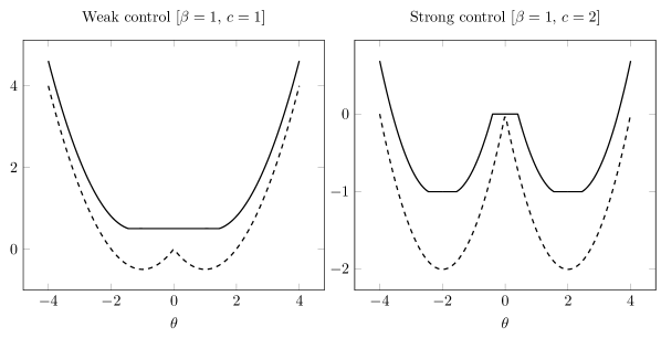
Figure 1. Representative graphs of $\frac{1}{2}\theta^{2}-c|\theta|$ (dashed) and $\overline{H}_{\beta,c}(\theta)$ (solid) against $\theta$ in each of the two control regimes. There is weak control if and only if $\beta\geq c^{2}/2$.

Proof.

We prove the existence of the limit in (3.1) separately in each of the two control regimes.

(a) (Weak control) Assume that $\beta\geq c^{2}/2$. By symmetry, it suffices to consider $\theta\geq 0$.

• If $0\leq\theta\leq c$, then the bounds (3.7) and (4.2) match,

  $$\overline{H}_{\beta,c}^{L}(\theta)=\overline{H}_{\beta,c}^{U}(\theta)=\beta-\frac{1}{2}c^{2},$$

  and taking the infimum in (3.1) over the set $\{\alpha^{(x_{*},h,y)}:\,0<h<h_{0},\ y>y_{0}\}$ for any $h_{0}>0$ and $y_{0}>0$ does not change the limit.

• If $\theta\geq 0$ and $\Lambda_{\beta}(\theta-c)=\beta$, then the bounds (3.4) and (4.2) match,

  $$\overline{H}_{\beta,c}^{L}(\theta)=\overline{H}_{\beta,c}^{U}(\theta)=\beta-\frac{1}{2}c^{2},$$

  and $\overleftarrow{\alpha}$ is asymptotically optimal.

• If $\theta>c$ and $\Lambda_{\beta}(\theta-c)>\beta$, then the bounds (3.4) and (4.3) match,

  $$\overline{H}_{\beta,c}^{L}(\theta)=\overline{H}_{\beta,c}^{U}(\theta)=\Lambda_{\beta}(\theta-c)-\frac{1}{2}c^{2},$$

  and $\overleftarrow{\alpha}$ is asymptotically optimal.

(b) (Strong control) Assume that $\beta<c^{2}/2$. By symmetry, it suffices to consider $\theta\geq 0$. Recall from Section 4.2 that there exists a unique $\bar{\theta}(\beta,c)\in(0,c)$ such that $\Lambda_{\beta}(\bar{\theta}(\beta,c)-c)=c^{2}/2$.

• If $0\leq\theta<\bar{\theta}(\beta,c)$, then the bounds (3.7), (4.5) and (4.6) match,

  $$\overline{H}_{\beta,c}^{L}(\theta)=\overline{H}_{\beta,c}^{U}(\theta)=0,$$

  and taking the infimum in (3.1) over the set $\{\alpha^{(x_{*},h,y)}:\,0<h<h_{0},\ y>y_{0}\}$ for any $h_{0}>0$ and $y_{0}>0$ does not change the limit.

• If $\theta\geq 0$ and $\Lambda_{\beta}(\theta-c)=\beta$, then the bounds (3.4) and (4.2) match,

  $$\overline{H}_{\beta,c}^{L}(\theta)=\overline{H}_{\beta,c}^{U}(\theta)=\beta-\frac{1}{2}c^{2},$$

  and $\overleftarrow{\alpha}$ is asymptotically optimal.

• If $\theta\geq\bar{\theta}(\beta,c)$ and $\Lambda_{\beta}(\theta-c)>\beta$, then the bounds (3.4) and (4.3) match,

  $$\overline{H}_{\beta,c}^{L}(\theta)=\overline{H}_{\beta,c}^{U}(\theta)=\Lambda_{\beta}(\theta-c)-\frac{1}{2}c^{2},$$

  and $\overleftarrow{\alpha}$ is asymptotically optimal.∎

5. Homogenization

In this section, we first state (and give references to) existence and uniqueness results for viscosity solutions to the Cauchy problems we have introduced in Section 1.1, then provide the control representation (5.5)-(5.6) for $v_{\theta}$ that we have mentioned there, and finally use (5.6) to prove our homogenization results (Theorem 1.2 and Corollary 1.4). We assume throughout the section that $V$ satisfies (1.3), (1.4) and (1.5). Since we work directly with the control representation rather than the equations themselves, we omit the definition of a viscosity solution and refer the reader to [CIL92, FS06].

5.1. Existence and uniqueness

The following results are well known in very general settings (see, for instance, [CIL92, CL86]). We state them here exactly in the form we need and give precise references for the convenience of the reader.

Lemma 5.1.

For every $g\in\text{UC}(\mathbb{R})$, $\varepsilon>0$ and $\omega\in\Omega$, the viscous Hamilton-Jacobi equation (1.1) subject to the initial condition $g$ has a unique viscosity solution $u^{\varepsilon}_{g}$ in $\text{UC}([0,\infty)\times\mathbb{R})$.

Proof.

For every $\omega\in\Omega$, the Hamiltonian $H_{\beta,c}(p,T_{x}\omega)=\frac{1}{2}p^{2}-c|p|+\beta V(T_{x}\omega)$ has the following three properties. First,

(5.1) $$\frac{1}{4}p^{2}-c^{2}\leq\frac{1}{2}p^{2}-c|p|\leq H_{\beta,c}(p,T_{x}\omega)\leq\frac{1}{2}p^{2}+\beta$$

for every $(p,x)\in\mathbb{R}\times\mathbb{R}$ since $0\leq(\frac{1}{2}|p|-c)^{2}=\frac{1}{4}p^{2}+c^{2}-c|p|$ and $V(T_{x}\omega)\in[0,1]$ by 1.3. Second,

(5.2) $$x\mapsto H_{\beta,c}(p,T_{x}\omega)$$ is Lipschitz continuous

by (1.4). Third,

(5.3) $$|H_{\beta,c}(p,T_{x}\omega)-H_{\beta,c}(q,T_{x}\omega)|=\left|\frac{1}{2}(|p|+|q|)-c\right|||p|-|q||\leq\left(\frac{1}{2}(|p|+|q|)+c\right)|p-q|$$

for every $p,q\in\mathbb{R}$. The desired result follows from [DK17, Theorem 2.8]. ∎

Lemma 5.2.

For every $g\in\text{UC}(\mathbb{R})$, the inviscid Hamilton-Jacobi equation (1.6) subject to the initial condition $g$ has a unique viscosity solution $\overline{u}_{g}$ in $\text{UC}([0,\infty)\times\mathbb{R})$.

Proof.

It is clear from (4.7)-(4.8) that the Hamiltonian $\overline{H}_{\beta,c}(p)$ is locally uniformly continuous in $p$. Moreover,

$$\frac{1}{4}p^{2}-c^{2}\leq\frac{1}{2}p^{2}-c|p|\leq\overline{H}_{\beta,c}(p)\leq\Lambda_{\beta}(p)\leq\frac{1}{2}p^{2}+\beta$$

for every $p\in\mathbb{R}$. Here, the first inequality is as in (5.1), the second inequality is easy to check by taking $\beta=0$ (see also Figure 1), the third inequality holds since $\alpha\equiv 0\in\mathcal{P}_{c}$, and the last inequality is part of Proposition 2.10(b). The desired result follows from [DK17, Theorem 2.5]. ∎

5.2. Control representation

For every $\theta\in\mathbb{R}$, $\varepsilon>0$, $(t,x)\in[0,\infty)\times\mathbb{R}$ and $\omega\in\Omega$, we will write $u_{\theta}^{\varepsilon}(t,x,\omega)$ to denote $u_{g}^{\varepsilon}(t,x,\omega)$ (see Lemma 5.1) when $g(x)=\theta x$. Note that

(5.4) $$u^{\varepsilon}_{\theta}(t,x,\omega)=\varepsilon u^{1}_{\theta}(t/\varepsilon,x/\varepsilon,\omega)$$

by the uniqueness part of Lemma 5.1. With this notation, we define

(5.5) $$v_{\theta}(t,x,\omega) =e^{u^{1}_{\theta}(t,x,\omega)}\quad\text{and}$$

$$\tilde{v}_{\theta}(t,x,\omega) =\inf_{\alpha\in\mathcal{P}_{c}}E_{x}\left[e^{\beta\int_{0}^{t}V(T_{X_{s}^{\alpha}}\omega)ds+\theta X_{t}^{\alpha}}\right].$$

Lemma 5.3.

For every $\theta\in\mathbb{R}$, $(t,x)\in[0,\infty)\times\mathbb{R}$ and $\omega\in\Omega$,

(5.6) $$v_{\theta}(t,x,\omega)=\tilde{v}_{\theta}(t,x,\omega).$$

Proof.

$\tilde{v}_{\theta}(t,x,\omega)$ is the value function of a finite horizon, risk-sensitive stochastic optimal control problem with running payoff function $x\mapsto\beta V(T_{x}\omega)$ and terminal payoff function $x\mapsto e^{\theta x}$. See [FS06, Chapter 6] for background. As we now show, $\tilde{v}_{\theta}$ is a viscosity solution of the associated Bellman equation

(5.7) $$\frac{\partial v}{\partial t} =\frac{1}{2}\frac{\partial^{2}v}{\partial x^{2}}+\inf_{|a|\leq c}\left(a\frac{\partial v}{\partial x}\right)+\beta V(T_{x}\omega)v$$

$$=\frac{1}{2}\frac{\partial^{2}v}{\partial x^{2}}-c\left|\frac{\partial v}{\partial x}\right|+\beta V(T_{x}\omega)v,\quad(t,x)\in(0,\infty)\times\mathbb{R}.$$

Indeed, when $\theta=0$ (i.e. the terminal payoff function is identically equal to $1$), the last statement follows directly from [FS06, Chapter 6, Theorem 8.1] which is applicable by our assumptions (1.3) and (1.4). On the other hand, when $\theta\neq 0$, we can absorb the terminal payoff into the running payoff as follows. For every $\alpha\in\mathcal{P}_{c}$,

$$E_{x}\left[e^{\beta\int_{0}^{t}V(T_{X_{s}^{\alpha}}\omega)ds+\theta X_{t}^{\alpha}}\right]=E_{x}\left[e^{\int_{0}^{t}[\beta V(T_{X_{s}^{\theta+\alpha}}\omega)+\theta\alpha_{s}+\frac{1}{2}\theta^{2}]ds}\right]e^{\theta x}$$

by Girsanov’s theorem. Here, $(\theta+\alpha)_{s}=\theta+\alpha_{s}$. Therefore,

$$\tilde{v}_{\theta}(t,x,\omega) =\inf_{\alpha\in\mathcal{P}_{c}}E_{x}\left[e^{\int_{0}^{t}[\beta V(T_{X_{s}^{\theta+\alpha}}\omega)+\theta\alpha_{s}+\frac{1}{2}\theta^{2}]ds}\right]e^{\theta x}$$

$$=\inf_{\alpha\in\mathcal{P}[\theta-c,\theta+c]}E_{x}\left[e^{\int_{0}^{t}[\beta V(T_{X_{s}^{\alpha}}\omega)+\theta\alpha_{s}-\frac{1}{2}\theta^{2}]ds}\right]e^{\theta x},$$

where

$${\mathcal{P}}[a,b]=\{\alpha=(\alpha_{s})_{s\geq 0}:\ \alpha\ \text{is $[a,b]$-valued and $\mathcal{G}_{s}$-progressively measurable}\}.$$

Now [FS06, Chapter 6, Theorem 8.1] is applicable and $\tilde{v}_{\theta}(t,x,\omega)e^{-\theta x}$ is a viscosity solution of

(5.8) $$\frac{\partial v}{\partial t}=\frac{1}{2}\frac{\partial^{2}v}{\partial x^{2}}+\inf_{|a-\theta|\leq c}\left(a\frac{\partial v}{\partial x}+a\theta v\right)+\left(\beta V(T_{x}\omega)-\frac{1}{2}\theta^{2}\right)v.$$

Expressing the derivatives of $\tilde{v}_{\theta}(t,x,\omega)$ in terms of those of $\tilde{v}_{\theta}(t,x,\omega)e^{-\theta x}$, we deduce that $\tilde{v}_{\theta}$ is a viscosity solution of (5.7).

Applying the inverse Hopf-Cole transformation to (5.8) (see [FS06, Chapter 6, Corollary 8.1]) and arranging the terms, we see that $\log\tilde{v}_{\theta}(t,x,\omega)-\theta x$ is a viscosity solution of

(5.9) $$\frac{\partial u}{\partial t}=\frac{1}{2}\frac{\partial^{2}u}{\partial x^{2}}+H_{\beta,c}\left(\theta+\frac{\partial u}{\partial x},T_{x}\omega\right),\quad(t,x)\in(0,\infty)\times\mathbb{R}.$$

Hence, $\log\tilde{v}_{\theta}$ is a viscosity solution of (1.1) with $\varepsilon=1$ and $\log\tilde{v}_{\theta}(0,x,\omega)=\theta x$. By Lemma 5.4 (see below) and the uniqueness part of Lemma 5.1, we deduce that $u_{\theta}^{1}=\log\tilde{v}_{\theta}$. Consequently, $v_{\theta}=e^{u_{\theta}^{1}}=\tilde{v}_{\theta}$. ∎

Lemma 5.4.

There exists a constant $\kappa$ depending only on $\beta$, $c$, $\theta$ and the Lipschitz constant of $x\mapsto V(T_{x}\omega)$ such that

$$|\log\tilde{v}_{\theta}(s,x,\omega)-\log\tilde{v}_{\theta}(t,y,\omega)|\leq\kappa(|s-t|+|x-y|)$$

for all $s,t\geq 0$, $x,y\in\mathbb{R}$ and $\omega\in\Omega$.

Proof.

Recall from the proof of Lemma 5.3 that $\log\tilde{v}_{\theta}(t,x,\omega)-\theta x$ is a viscosity solution of (5.9) and $\log\tilde{v}_{\theta}(0,x,\omega)-\theta x=0$. It follows from [Dav16, Theorem 3.2] that $\log\tilde{v}_{\theta}(t,x,\omega)-\theta x$ is Lipschitz continuous in $t\in[0,\infty)$ and $x\in\mathbb{R}$ with a Lipschitz constant $\kappa^{\prime}$ that depends only on $\beta,c,\theta$ and the Lipschitz constant of $x\mapsto V(T_{x}\omega)$ (which is finite by (1.4)). This implies the desired result. ∎

Remark 5.5.

If $x\mapsto V(T_{x}\omega)$ is in $C_{b}^{2}(\mathbb{R})$, then $u_{\theta}^{\varepsilon}$ is in fact a classical solution of the Cauchy problem (1.1)-(1.2) with $g(x)=\theta x$. See [FS06, Chapter 6, Remark 8.1].

5.3. Proofs of the homogenization results

We are finally ready to combine our results on the effective Hamiltonian (see Section 2.3 for $c=0$ and Section 4.3 for $c>0$) with the control representation of $v_{\theta}$ (see Section 5.2).

Proof of Theorem 1.2.

Recall from the proof of Lemma 5.1 that $H_{\beta,c}$ satisfies (5.1), (5.2) and (5.3). For every $\theta\in\mathbb{R}$ and $\mathbb{P}$-a.e. $\omega$,

$$\lim_{\varepsilon\to 0}u_{\theta}^{\varepsilon}(1,0,\omega)=\lim_{\varepsilon\to 0}\varepsilon u^{1}_{\theta}(1/\varepsilon,0,\omega)=\lim_{t\to\infty}\inf_{\alpha\in\mathcal{P}_{c}}\frac{1}{t}\log E_{0}\left[e^{\beta\int_{0}^{t}V(T_{X_{s}^{\alpha}}\omega)ds+\theta X_{t}^{\alpha}}\right]=\overline{H}_{\beta,c}(\theta)$$

by (5.4) and Lemma 5.3. The last equality is shown in Theorem 2.9 (resp. Theorem 4.3) for $c=0$ (resp. $c>0$). The desired result follows from [DK17, Lemma 4.1] where the remaining condition (4.2) there holds by Lemma 5.4. ∎

Proof of Corollary 1.4.

Recall from the proof of Lemma 5.1 that $H_{\beta,c}$ satisfies (5.1), (5.2) and (5.3). The desired result follows from [DK17, Theorem 3.1] where the remaining condition (L) there holds by Lemma 5.4. ∎

Appendix A Some properties of the tilted free energy

Proof of Proposition 2.10.

(a) These three properties follow from $V(\cdot)\geq 0$, the symmetry of the law of BM and a standard application of Hölder’s inequality, respectively.

(b) Since $V(\cdot)\in[0,1]$,

$$\frac{1}{2}\theta^{2}=\frac{1}{t}\log E_{0}\left[e^{\theta X_{t}}\right]\leq\frac{1}{t}\log E_{0}\left[e^{\beta\int_{0}^{t}V(T_{X_{s}}\omega)ds+\theta X_{t}}\right]\leq\frac{1}{t}\log E_{0}\left[e^{\beta t+\theta X_{t}}\right]=\beta+\frac{1}{2}\theta^{2}.$$

Sending $t\to\infty$ and recalling from Theorem 2.9 that $\Lambda_{\beta}(\theta)\geq\beta$, we obtain the desired bounds.

(c) For every $h\in(0,1)$,

$$v_{\beta}^{\beta}(\omega,0;1) =E_{0}\left[e^{\beta\int_{0}^{\tau_{1}}[V(T_{X_{s}}\omega)-1]ds}\right]$$

$$\leq E_{0}\left[e^{\beta(h-1)L(\tau_{1},[0,1])}\right]{{\rm 1\mkern-1.5mu}\!{\rm I}}_{\{[0,1]\ \text{is an $h$-valley}\}}+{{\rm 1\mkern-1.5mu}\!{\rm I}}_{\{[0,1]\ \text{is not an $h$-valley}\}}.$$

Here, $L(t,[a,b])=\int_{0}^{t}{{\rm 1\mkern-1.5mu}\!{\rm I}}_{\{X_{s}\in[a,b]\}}ds$ denotes the occupation time of BM on the interval $[a,b]$ up to time $t$. Since $P_{0}(L(\tau_{1},[0,1])>0)=1$, we have $E_{0}\left[e^{\beta(h-1)L(\tau_{1},[0,1])}\right]<1$. Therefore, $\mathbb{E}[\log v_{\beta}^{\beta}(\cdot,0;1)]<0$ by (1.5). Take any sufficiently small $\theta\geq 0$ so that

(A.1) $$\mathbb{E}[\log v_{\beta}^{\beta}(\cdot,0;1)]+\theta<0.$$

Recall from the proof of Lemma 2.5 (with $\lambda=\beta$) that

$$e^{t(\Lambda_{\beta}(\theta)-\beta)+o(t)}=E_{0}\left[e^{\beta\int_{0}^{t}V(T_{X_{s}}\omega)ds+\theta X_{t}}\right]e^{-t\beta}\leq\sum_{k=0}^{\infty}e^{\theta+\sum_{j=0}^{k-1}[\log v_{\beta}^{\beta}(T_{j}\omega,0;1)+\theta]}.$$

The RHS is a convergent series since the exponent in the kth term grows linearly in $k$ (with a negative sign) by (A.1) and the Birkhoff ergodic theorem. We deduce that $\Lambda_{\beta}(\theta)\leq\beta$ and conclude by appealing to parts (a) and (b).

(d) Recall from (2.6) that

$$F_{\beta,\theta}^{\lambda}(\omega,1)=-\log v_{\beta}^{\lambda}(\omega,0;1)-\theta=-\log E_{0}\left[e^{\beta\int_{0}^{\tau_{1}}V(T_{X_{s}}\omega)ds-\lambda\tau_{1}}\right]-\theta$$

for every $\omega\in\Omega$, $\theta>0$ and $\lambda\geq\beta$. Since $V(\cdot)\in[0,1]$, it follows from the dominated convergence theorem (DCT) that the function $\lambda\mapsto F_{\beta,\theta}^{\lambda}(\omega,1)$ is differentiable for $\lambda>\beta$. By a second application of the DCT, we deduce that the function $\lambda\mapsto\mathbb{E}[F_{\beta,\theta}^{\lambda}(\cdot,1)]$ is differentiable and

$$\frac{\partial}{\partial\lambda}\mathbb{E}[F_{\beta,\theta}^{\lambda}(\cdot,1)]=\mathbb{E}\left[\frac{E_{0}\left[\tau_{1}e^{\beta\int_{0}^{\tau_{1}}V(T_{X_{s}}\omega)ds-\lambda\tau_{1}}\right]}{E_{0}\left[e^{\beta\int_{0}^{\tau_{1}}V(T_{X_{s}}\omega)ds-\lambda\tau_{1}}\right]}\right]>0.$$

Using the DCT for a third time, we see that $\lambda\mapsto\mathbb{E}[F_{\beta,\theta}^{\lambda}(\cdot,1)]$ is continuously differentiable. The function $\theta\mapsto\mathbb{E}[F_{\beta,\theta}^{\lambda}(\cdot,1)]$ is linear, and hence continuously differentiable, too. Recall from Lemma 2.6 and Theorem 2.9 that

$$0=\mathbb{E}[F_{\beta,\theta}(\cdot,1)]=\mathbb{E}[F_{\beta,\theta}^{\lambda_{o}(\beta,\theta)}(\cdot,1)]=\mathbb{E}[F_{\beta,\theta}^{\Lambda_{\beta}(\theta)}(\cdot,1)]$$

for $\theta>0$ and $\Lambda_{\beta}(\theta)>\beta$. Thus, by the implicit function theorem, the function $\theta\mapsto\Lambda_{\beta}(\theta)$ is continuously differentiable on the set $\{\theta\in\mathbb{R}:\,\theta>0\ \text{and}\ \Lambda_{\beta}(\theta)>\beta\}$. Since $\Lambda_{\beta}(-\theta)=\Lambda_{\beta}(\theta)$ and $\Lambda_{\beta}(0)=\beta$ by parts (a) and (c), this concludes the proof.∎

References

• [AC15a] Scott N. Armstrong and Pierre Cardaliaguet. Quantitative stochastic homogenization of viscous Hamilton-Jacobi equations. Comm. Partial Differential Equations, 40(3):540–600, 2015.
• [AC15b] Scott N. Armstrong and Pierre Cardaliaguet. Stochastic homogenization of quasilinear Hamilton-Jacobi equations and geometric motions, April 2015. Eprint arXiv:math.PR/1504.02045. To appear, J. Eur. Math. Soc. (JEMS).
• [AS12] Scott N. Armstrong and Panagiotis E. Souganidis. Stochastic homogenization of Hamilton-Jacobi and degenerate Bellman equations in unbounded environments. J. Math. Pures Appl. (9), 97(5):460–504, 2012.
• [AS13] Scott N. Armstrong and Panagiotis E. Souganidis. Stochastic homogenization of level-set convex Hamilton-Jacobi equations. Int. Math. Res. Not. IMRN, (15):3420–3449, 2013.
• [AT14] Scott N. Armstrong and Hung V. Tran. Stochastic homogenization of viscous Hamilton-Jacobi equations and applications. Anal. PDE, 7(8):1969–2007, 2014.
• [ATY15] Scott N. Armstrong, Hung V. Tran, and Yifeng Yu. Stochastic homogenization of a nonconvex Hamilton-Jacobi equation. Calc. Var. Partial Differential Equations, 54(2):1507–1524, 2015.
• [ATY16] Scott N. Armstrong, Hung V. Tran, and Yifeng Yu. Stochastic homogenization of nonconvex Hamilton-Jacobi equations in one space dimension. J. Differential Equations, 261(5):2702–2737, 2016.
• [BL16] Yuri Bakhtin and Liying Li. Thermodynamic limit for directed polymers and stationary solutions of the Burgers equation, July 2016. Eprint arXiv:math.PR/1607.04864.
• [BLP78] Alain Bensoussan, Jacques-Louis Lions, and George Papanicolaou. Asymptotic analysis for periodic structures, volume 5 of Studies in Mathematics and its Applications. North-Holland Publishing Co., Amsterdam-New York, 1978.
• [CIL92] Michael G. Crandall, Hitoshi Ishii, and Pierre-Louis Lions. User’s guide to viscosity solutions of second order partial differential equations. Bull. Amer. Math. Soc. (N.S.), 27(1):1–67, 1992.
• [CL86] Michael G. Crandall and Pierre-Louis Lions. On existence and uniqueness of solutions of Hamilton-Jacobi equations. Nonlinear Anal., 10(4):353–370, 1986.
• [CS17] Pierre Cardaliaguet and Panagiotis E. Souganidis. On the existence of correctors for the stochastic homogenization of viscous Hamilton–Jacobi equations. C. R. Math. Acad. Sci. Paris, 355(7):786–794, 2017.
• [Dav16] Andrea Davini. Existence and uniqueness of solutions to parabolic equations with superlinear Hamiltonians, August 2016. Eprint arXiv:math.PR/1608.04043.
• [DH14] Michael Damron and Jack Hanson. Busemann functions and infinite geodesics in two-dimensional first-passage percolation. Comm. Math. Phys., 325(3):917–963, 2014.
• [DK17] Andrea Davini and Elena Kosygina. Homogenization of viscous and non-viscous HJ equations: a remark and an application. Calc. Var. Partial Differential Equations, 56(4):Art. 95, 21, 2017.
• [DS09] Andrea Davini and Antonio Siconolfi. Exact and approximate correctors for stochastic Hamiltonians: the 1-dimensional case. Math. Ann., 345(4):749–782, 2009.
• [DS12] Andrea Davini and Antonio Siconolfi. Weak KAM Theory topics in the stationary ergodic setting. Calc. Var. Partial Differential Equations, 44(3-4):319–350, 2012.
• [Dyn02] E. B. Dynkin. Diffusions, superdiffusions and partial differential equations, volume 50 of American Mathematical Society Colloquium Publications. American Mathematical Society, Providence, RI, 2002.
• [Eva92] Lawrence C. Evans. Periodic homogenisation of certain fully nonlinear partial differential equations. Proc. Roy. Soc. Edinburgh Sect. A, 120(3-4):245–265, 1992.
• [FKZ15] Martin Forde, Rohini Kumar, and Hongzhong Zhang. Large deviations for the boundary local time of doubly reflected Brownian motion. Statist. Probab. Lett., 96:262–268, 2015.
• [FS89] Wendell H. Fleming and Panagiotis E. Souganidis. On the existence of value functions of two-player, zero-sum stochastic differential games. Indiana Univ. Math. J., 38(2):293–314, 1989.
• [FS06] Wendell H. Fleming and H. Mete Soner. Controlled Markov processes and viscosity solutions, volume 25 of Stochastic Modelling and Applied Probability. Springer, New York, second edition, 2006.
• [FS16] William M. Feldman and Panagiotis E. Souganidis. Homogenization and non-homogenization of certain non-convex Hamilton-Jacobi equations, September 2016. Eprint arXiv:math.PR/1609.09410.
• [Gao16] Hongwei Gao. Random homogenization of coercive Hamilton-Jacobi equations in 1d. Calc. Var. Partial Differential Equations, 55(2):Paper No. 30, 39, 2016.
• [GRAS16] Nicos Georgiou, Firas Rassoul-Agha, and Timo Seppäläinen. Variational formulas and cocycle solutions for directed polymer and percolation models. Comm. Math. Phys., 346(2):741–779, 2016.
• [JKO94] V. V. Jikov, S. M. Kozlov, and O. A. Oleĭnik. Homogenization of differential operators and integral functionals. Springer-Verlag, Berlin, 1994. Translated from the Russian by G. A. Yosifian [G. A. Iosif’yan].
• [Kri16] Arjun Krishnan. Variational formula for the time constant of first-passage percolation. Comm. Pure Appl. Math., 69(10):1984–2012, 2016.
• [KRV06] Elena Kosygina, Fraydoun Rezakhanlou, and S. R. S. Varadhan. Stochastic homogenization of Hamilton-Jacobi-Bellman equations. Comm. Pure Appl. Math., 59(10):1489–1521, 2006.
• [KS91] Ioannis Karatzas and Steven E. Shreve. Brownian motion and stochastic calculus, volume 113 of Graduate Texts in Mathematics. Springer-Verlag, New York, second edition, 1991.
• [LPV87] Pierre-Louis Lions, George Papanicolaou, and S. R. S. Varadhan. Homogenization of Hamilton-Jacobi equation. unpublished preprint, circa 1987.
• [LS03] Pierre-Louis Lions and Panagiotis E. Souganidis. Correctors for the homogenization of Hamilton-Jacobi equations in the stationary ergodic setting. Comm. Pure Appl. Math., 56(10):1501–1524, 2003.
• [LS05] Pierre-Louis Lions and Panagiotis E. Souganidis. Homogenization of “viscous” Hamilton-Jacobi equations in stationary ergodic media. Comm. Partial Differential Equations, 30(1-3):335–375, 2005.
• [LS10] Pierre-Louis Lions and Panagiotis E. Souganidis. Stochastic homogenization of Hamilton-Jacobi and “viscous”-Hamilton-Jacobi equations with convex nonlinearities—revisited. Commun. Math. Sci., 8(2):627–637, 2010.
• [QTY17] Jianliang Qian, Hung V. Tran, and Yifeng Yu. Min-max formulas and other properties of certain classes of nonconvex effective Hamiltonians, January 2017. Eprint arXiv:math.PR/1701.01065.
• [RT00] Fraydoun Rezakhanlou and James E. Tarver. Homogenization for stochastic Hamilton-Jacobi equations. Arch. Ration. Mech. Anal., 151(4):277–309, 2000.
• [RW00] L. C. G. Rogers and David Williams. Diffusions, Markov processes, and martingales. Vol. 2. Cambridge Mathematical Library. Cambridge University Press, Cambridge, 2000. Itô calculus, Reprint of the second (1994) edition.
• [RY99] Daniel Revuz and Marc Yor. Continuous martingales and Brownian motion, volume 293 of Grundlehren der Mathematischen Wissenschaften [Fundamental Principles of Mathematical Sciences]. Springer-Verlag, Berlin, third edition, 1999.
• [Szn94] Alain-Sol Sznitman. Shape theorem, Lyapounov exponents, and large deviations for Brownian motion in a Poissonian potential. Comm. Pure Appl. Math., 47(12):1655–1688, 1994.
• [Var07] S. R. S. Varadhan. Stochastic processes, volume 16 of Courant Lecture Notes in Mathematics. Courant Institute of Mathematical Sciences, New York; American Mathematical Society, Providence, RI, 2007.
• [Yil11] Atilla Yilmaz. Harmonic functions, $h$-transform and large deviations for random walks in random environments in dimensions four and higher. Ann. Probab., 39(2):471–506, 2011.
• [YZ17] Atilla Yilmaz and Ofer Zeitouni. Nonconvex homogenization for one-dimensional controlled random walks in random potential, May 2017. Eprint arXiv:math.PR/1705.07613.
• [Zil15] Bruno Ziliotto. Stochastic homogenization of nonconvex Hamilton-Jacobi equations: a counterexample, December 2015. Eprint arXiv:math.AP/1512.06375. To appear, Comm. Pure Appl. Math.
• [Zvo74] A. K. Zvonkin. A transformation of the phase space of a diffusion process that will remove the drift. Mat. Sb. (N.S.), 93(135):129–149, 152, 1974.