Boundary charges and integral identities for solitons in $(d+1)$-dimensional field theories

Abstract

We establish a 3-parameter family of integral identities to be used on a class of theories possessing solitons with spherical symmetry in $d$ spatial dimensions. The construction provides five boundary charges that are related to certain integrals of the profile functions of the solitons in question. The framework is quite generic and we give examples of both topological defects (like vortices and monopoles) and topological textures (like Skyrmions) in 2 and 3 dimensions. The class of theories considered here is based on a kinetic term and three functionals often encountered in reduced Lagrangians for solitons. One particularly interesting case provides a generalization of the well-known Pohozaev identity. Our construction, however, is fundamentally different from scaling arguments behind Derrick’s theorem and virial relations. For BPS vortices, we find interestingly an infinity of integrals simply related to the topological winding number.

1 Introduction

Solitons play an important role in non-perturbative physics of all kinds. Except for a few special cases, such as self-dual instantons or dimensional reductions thereof, solitonic systems are often not integrable in more than one codimension. Vortices at critical coupling are described by the Taubes equation Taubes:1979tm which is not integrable. The exception, however, is the case where they are placed on a hyperbolic plane of a particular constant curvature and the Taubes equation is modified into the Liouville equation and hence becomes integrable Witten:1976ck . This case corresponds, however, to the self-dual instanton equation on the background $S^{2}\times\mathbb{H}^{2}$ and thus it is not surprising that it is integrable.

Hence most soliton solutions can only be obtained by means of numerical techniques and in case of numerically challenging parts of the parameter space, mathematical identities other than the equation of motion can be useful to check the validity and precision of the obtained numerical solutions, because the former often involve lower-order derivatives.

For simplicity, we focus on a simple class of theories with spherical symmetry, that consists of a single profile function, $f$, which has a Lagrangian description that involves a standard kinetic term, two functionals of $f$: one purely dependent on the field and one that also allows for the coordinate ($r$), and finally a modified kinetic term, that is simply parametrized by a functional of $f$ and $r$. The potential term that allows for a dependence on $r$ can be thought of as a standard kinetic term, where the derivatives act on the angular parts of the underlying field configuration; for sigma model fields, this looks in the reduced Lagrangian like an $r$-dependent potential. Since we will be interested in topological solitons, we will not consider time dependence; this makes our results applicable for both relativistic as well as non-relativistic theories. The reason for imposing spherical symmetry is simply to reduce the equation of motion to a one-dimensional one. We do, however, keep the number of spatial dimensions general, so that spherically symmetric systems in $d$ dimensions are treated on equal footing.

In practice our construction is based on the equation of motion along the radial coordinate, multiplied by an appropriately chosen weight function, that allows us to turn the standard “conjugate momentum”, $\frac{\partial\mathcal{L}}{\partial f^{\prime}}$, into a generalized function which remains as a boundary term (total derivative) in the equation. Once we integrate the equation, we get the first boundary charge, which we shall denote as the type-0 boundary charge.

A more interesting outcome of our construction of identities than simply making relations that can be used for checking numerical solutions, is that – in the class of theories that we are considering – we find five different types of boundary terms, yielding the possibility of picking up what we call boundary charges. The boundary charge consists of some combination of solution parameters, Lagrangian parameters, coupling constants or boundary conditions – evaluated at the endpoint(s) of the integration range. We would like to promote the boundary charges to be thought of as topological boundary charges, although we do not have a mathematical understanding (definition) of them yet. There are two reasons for this promotion; the first is due to the fact that any angular dependence in the higher-dimensional soliton will often contribute the winding number or topological degree to exactly these boundary charges. The second reason is the similarity of the boundary charges and so-called domain wall topological charges (although in the case of the domain wall, it is not a difference of the potential, but of the superpotential, evaluated on the endpoints of the field values).

After setting up the general framework of identities and illustrating various flavors or simplifications of the main identity, we consider some examples of solitons in 2 and 3 dimensions. We obtain many interesting relations; in particular, we find a generalization of the Pohozaev identity Pohozaev:1965 , see e.g. Eq. (24) below. The generalization picks up three different boundary charges, that we call type 0, type IIa and type IIb, respectively, and relates them to the potential energy of the system as well as other terms that are generically non-vanishing with respect to Derrick scaling Derrick:1964ww (that means classically non-conformal).

The most general form of our identity is a 3-parameter family of relations that nontrivially provide different integrals of the fields. The three parameters can be used to pick up the desired boundary charges of the theory at hand (if possible), but also it can be used to avoid unwanted divergences that often plague global solitons (as a consequence of Derrick’s theorem).

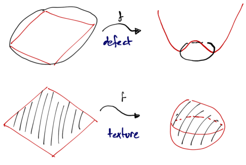
Figure 1: Topological defects versus topological textures.

Since the boundary charges crucially depend on the solutions and in turn on their boundary conditions, it will prove useful to define the following notation for topological solitons (which we will refer to throughout the paper): we distinguish between topological defects and topological textures, see Fig. 1. The topological defect in $d$ spatial dimensions, is defined by having a nontrivial $(d-1)$-th homotopy group of the target space of the theory

$$\pi_{d-1}(G/H),$$ (1)

because the soliton solution is a map from the boundary of space $\partial\mathbb{R}^{d}\simeq S^{d-1}$ to $G/H$, where $G$ is an internal symmetry group and $H$ is a stabilizer. The prime example is a vortex in $d=2$ dimensions in a theory where an internal U(1) symmetry is completely broken

$$\pi_{1}(S^{1})=\mathbb{Z},$$ (2)

which constitutes the group of integers.

The topological texture, on the other hand, is by construction a map of the whole space with infinity compactified to a point, $\mathbb{R}^{d}\cup\{\infty\}\simeq S^{d}$ to the target space $G/H$. This yields the homotopy group for a topological texture

$$\pi_{d}(G/H),$$ (3)

which is clearly different from that of a defect.

For BPS vortices of both standard Abelian-Higgs type and Chern-Simons type, we find type-0 boundary charges proportional to the winding number, due to the logarithmic singularity at the origin of the auxiliary profile function. We find what we later will define as type-II boundary charges for global vortices, the Skyrme vortices and the global monopoles, but not for the topological textures (such as the baby Skyrmions and the Skyrmions). On the other hand, we find type-I boundary charges for the baby Skyrmions, the Skyrme vortices and the Skyrmions, viz. only for theories with higher-order derivative terms (for the definition of the types of boundary charges, see the next section).

A comment in store is about the origin of the boundary charges. We would like to stress that naive scaling arguments may miss the boundary charges and hence, in certain cases with nontrivial boundary conditions or topological winding at infinity, will get the wrong answer. Therefore, our relations are not simply based on scaling arguments, like Derrick’s theorem or virial theorems. Our identities are also not directly related to the Noether theorem. As mentioned above, the exact mathematical origin of the boundary charges are not yet known.

Although the relations we find are interesting themselves, we flesh out many details of the framework of finding the boundary charges in the hope that the interested reader will better understand the mechanisms at work and perhaps further generalize the framework.

The paper is organized as follows. In Sec. 2 we derive the identity and illustrate the cases giving rise to the five boundary charges as well as many cases that simplify the main identity for our class of theories. Secs. 3 and 4 illustrate the framework of identities with examples of topological solitons of both defect type and texture type in two and three dimensions, respectively. Finally, Sec. 5 concludes the paper with a discussion and outlook on how the results can be generalized. Some selected numerical checks are delegated to appendix A.

2 The identity

Let us consider the static Lagrangian density in $d$ spatial dimensions (i.e on $\mathbb{R}^{d}$) of the form

$$\mathcal{L}[f,f^{\prime},r]=-\frac{1}{2}f^{{}^{\prime}2}-F[f,r]-\frac{1}{2}G[f,r]f^{{}^{\prime}2}-V[f],$$ (4)

where $f=f(r)$ is a radial profile function and $f^{\prime}\equiv\frac{\operatorname{d}\!{f}}{\operatorname{d}\!{r}}$. The Euler-Lagrange equation associated with the action $\int_{0}^{\infty}\operatorname{d}\!{r}\;r^{d-1}\mathcal{L}$ reads

$$\frac{1}{r^{d-1}}\frac{\operatorname{d}\!{}}{\operatorname{d}\!{r}}\left(r^{d-1}(1+G)f^{\prime}\right)-\frac{\partial F}{\partial f}-\frac{1}{2}\frac{\partial G}{\partial f}f^{{}^{\prime}2}-\frac{\partial V}{\partial f}=0.$$ (5)

The basic construction of our class of identities is to multiply the equation of motion by $r^{(d-1)\kappa}f^{{}^{\prime}\mu-1}(1+G)^{\nu-1}$ and rearrange the terms into total derivatives where possible

$$\frac{1}{\lambda}\frac{\operatorname{d}\!{}}{\operatorname{d}\!{r}}\left(r^{(d-1)\kappa}(1+G)^{\nu}f^{{}^{\prime}\mu}\right)+(d-1)\left(1-\frac{\kappa}{\lambda}\right)r^{(d-1)\kappa-1}(1+G)^{\nu}f^{{}^{\prime}\mu}$$

$$+\left(1-\frac{\mu}{\lambda}\right)r^{(d-1)\kappa}(1+G)^{\nu}f^{{}^{\prime}\mu-1}f^{\prime\prime}+\left(\frac{1}{2}-\frac{\nu}{\lambda}\right)r^{(d-1)\kappa}(1+G)^{\nu-1}\frac{\partial G}{\partial f}f^{{}^{\prime}\mu+1}$$

$$+\left(1-\frac{\nu}{\lambda}\right)r^{(d-1)\kappa}(1+G)^{\nu-1}\frac{\partial G}{\partial r}f^{{}^{\prime}\mu}-r^{(d-1)\kappa}\frac{\partial F}{\partial f}(1+G)^{\nu-1}f^{{}^{\prime}\mu-1}$$

$$-r^{(d-1)\kappa}(1+G)^{\nu-1}\frac{\partial V}{\partial f}f^{{}^{\prime}\mu-1}=0.$$ (6)

In the above equation, we formally take all parameters such that all terms are real and well-defined quantities. The first term, proportional to $1/\lambda$ is added as a total derivative and subtracted again as integrals of the derivative acting on each factor. $\lambda$ should be chosen to be equal to one of the other three parameters ($\kappa$, $\mu$ or $\nu$), see below. Integrating the above equation with respect to $r$ yields

$$\left.\frac{1}{\lambda}r^{(d-1)\kappa}(1+G)^{\nu}f^{{}^{\prime}\mu}\right|_{0}^{\infty}+(d-1)\left(1-\frac{\kappa}{\lambda}\right)\int_{0}^{\infty}\operatorname{d}\!{r}\;r^{(d-1)\kappa-1}(1+G)^{\nu}f^{{}^{\prime}\mu}$$

$$+\left(1-\frac{\mu}{\lambda}\right)\int_{0}^{\infty}\operatorname{d}\!{r}\;r^{(d-1)\kappa}(1+G)^{\nu}f^{{}^{\prime}\mu-1}f^{\prime\prime}+\left(\frac{1}{2}-\frac{\nu}{\lambda}\right)\int_{0}^{\infty}\operatorname{d}\!{r}\;r^{(d-1)\kappa}(1+G)^{\nu-1}\frac{\partial G}{\partial f}f^{{}^{\prime}\mu+1}$$

$$+\left(1-\frac{\nu}{\lambda}\right)\int_{0}^{\infty}\operatorname{d}\!{r}\;r^{(d-1)\kappa}(1+G)^{\nu-1}\frac{\partial G}{\partial r}f^{{}^{\prime}\mu}-\int_{0}^{\infty}\operatorname{d}\!{r}\;r^{(d-1)\kappa}\frac{\partial F}{\partial f}(1+G)^{\nu-1}f^{{}^{\prime}\mu-1}$$

$$-\int_{0}^{\infty}\operatorname{d}\!{r}\;r^{(d-1)\kappa}(1+G)^{\nu-1}\frac{\partial V}{\partial f}f^{{}^{\prime}\mu-1}=0.$$ (7)

which is the basic identity and $\kappa,\mu,\nu$ and $\lambda$ are real (not necessarily integer) parameters. Although it is very complicated in its most general form, we will see that certain choices for $\kappa,\mu,\nu$ and $\lambda$, will give interesting subclasses of integral identities depending on the theory under study.

The first boundary term is found by integrating the total derivative in Eq. (6); we will call this the boundary charge of type 0.

Keeping $\lambda$ as a parameter is the most general case. One can always integrate the third term by parts to get rid of $f^{\prime\prime}$; that is, however, exactly the same as setting $\lambda=\mu$, which also eliminates $f^{\prime\prime}$ from the identity. Not having to know $f^{\prime\prime}$ can be advantageous numerically, because it is often easier to calculate $f^{\prime}$ than $f^{\prime\prime}$. $\lambda$ is not a genuine parameter on the same footing as $\kappa$, $\mu$ and $\nu$, because the terms that $1/\lambda$ multiplies add up to zero. The purpose of $\lambda$ is to leave the choice of setting $\lambda=\mu$, $\lambda=\kappa$ or $\lambda=\nu$ open and $\lambda$ is thus left as a free parameter to make a unified framework of identities.

In the construction, we have assumed a standard kinetic term ($-\tfrac{1}{2}f^{\prime 2}$) in the Lagrangian density. If such term is not present, a simple substitution can be made to get the appropriate identity: $(1+G)\to G$.

Let us discuss different possibilities where the general identity (7) simplifies:

1. $\lambda=\kappa$ makes the second term vanish,

2. $\lambda=\mu$ makes the third term vanish,

3. $\lambda=2\nu$ eliminates the fourth term; if $G$ is a function of only $f$, this may be useful,

4. $\lambda=\nu$ eliminates the fifth term; if $G$ is a function of only $r$, this may be useful,

5. $G=0$ simplifies all terms and eliminates the second and third terms,

6. if $G\neq 0$, then $\nu=1$ simplifies the $(1+G)$ factors in the last four terms,

7. $\mu=1$ allows for integration by parts of the second and fifth terms,

8. $\mu=2$ allows for the possibility to rewrite the last (two) term(s) into an integral over $V$ (and $F$); this is desirable if one wants to determine the potential energy.

Let us write out the simplified identities in turn, starting with the identity I ($\lambda=\kappa$):

$$\left.\frac{1}{\kappa}r^{(d-1)\kappa}(1+G)^{\nu}f^{{}^{\prime}\mu}\right|_{0}^{\infty}+\left(1-\frac{\mu}{\kappa}\right)\int_{0}^{\infty}\operatorname{d}\!{r}\;r^{(d-1)\kappa}(1+G)^{\nu}f^{{}^{\prime}\mu-1}f^{\prime\prime}$$

$$+\left(\frac{1}{2}-\frac{\nu}{\kappa}\right)\int_{0}^{\infty}\operatorname{d}\!{r}\;r^{(d-1)\kappa}(1+G)^{\nu-1}\frac{\partial G}{\partial f}f^{{}^{\prime}\mu+1}$$

$$+\left(1-\frac{\nu}{\kappa}\right)\int_{0}^{\infty}\operatorname{d}\!{r}\;r^{(d-1)\kappa}(1+G)^{\nu-1}\frac{\partial G}{\partial r}f^{{}^{\prime}\mu}-\int_{0}^{\infty}\operatorname{d}\!{r}\;r^{(d-1)\kappa}\frac{\partial F}{\partial f}(1+G)^{\nu-1}f^{{}^{\prime}\mu-1}$$

$$-\int_{0}^{\infty}\operatorname{d}\!{r}\;r^{(d-1)\kappa}(1+G)^{\nu-1}\frac{\partial V}{\partial f}f^{{}^{\prime}\mu-1}=0.$$ (8)

Identity II ($\lambda=\mu$):

$$\left.\frac{1}{\mu}r^{(d-1)\kappa}(1+G)^{\nu}f^{{}^{\prime}\mu}\right|_{0}^{\infty}+(d-1)\left(1-\frac{\kappa}{\mu}\right)\int_{0}^{\infty}\operatorname{d}\!{r}\;r^{(d-1)\kappa-1}(1+G)^{\nu}f^{{}^{\prime}\mu}$$

$$+\left(\frac{1}{2}-\frac{\nu}{\mu}\right)\int_{0}^{\infty}\operatorname{d}\!{r}\;r^{(d-1)\kappa}(1+G)^{\nu-1}\frac{\partial G}{\partial f}f^{{}^{\prime}\mu+1}$$

$$+\left(1-\frac{\nu}{\mu}\right)\int_{0}^{\infty}\operatorname{d}\!{r}\;r^{(d-1)\kappa}(1+G)^{\nu-1}\frac{\partial G}{\partial r}f^{{}^{\prime}\mu}-\int_{0}^{\infty}\operatorname{d}\!{r}\;r^{(d-1)\kappa}\frac{\partial F}{\partial f}(1+G)^{\nu-1}f^{{}^{\prime}\mu-1}$$

$$-\int_{0}^{\infty}\operatorname{d}\!{r}\;r^{(d-1)\kappa}(1+G)^{\nu-1}\frac{\partial V}{\partial f}f^{{}^{\prime}\mu-1}=0.$$ (9)

Identity III ($\lambda=2\nu$):

$$\left.\frac{1}{2\nu}r^{(d-1)\kappa}(1+G)^{\nu}f^{{}^{\prime}\mu}\right|_{0}^{\infty}+(d-1)\left(1-\frac{\kappa}{2\nu}\right)\int_{0}^{\infty}\operatorname{d}\!{r}\;r^{(d-1)\kappa-1}(1+G)^{\nu}f^{{}^{\prime}\mu}$$

$$+\left(1-\frac{\mu}{2\nu}\right)\int_{0}^{\infty}\operatorname{d}\!{r}\;r^{(d-1)\kappa}(1+G)^{\nu}f^{{}^{\prime}\mu-1}f^{\prime\prime}+\frac{1}{2}\int_{0}^{\infty}\operatorname{d}\!{r}\;r^{(d-1)\kappa}(1+G)^{\nu-1}\frac{\partial G}{\partial r}f^{{}^{\prime}\mu}$$

$$-\int_{0}^{\infty}\operatorname{d}\!{r}\;r^{(d-1)\kappa}\frac{\partial F}{\partial f}(1+G)^{\nu-1}f^{{}^{\prime}\mu-1}-\int_{0}^{\infty}\operatorname{d}\!{r}\;r^{(d-1)\kappa}(1+G)^{\nu-1}\frac{\partial V}{\partial f}f^{{}^{\prime}\mu-1}=0.$$ (10)

Identity IV ($\lambda=\nu$):

$$\left.\frac{1}{\nu}r^{(d-1)\kappa}(1+G)^{\nu}f^{{}^{\prime}\mu}\right|_{0}^{\infty}+(d-1)\left(1-\frac{\kappa}{\nu}\right)\int_{0}^{\infty}\operatorname{d}\!{r}\;r^{(d-1)\kappa-1}(1+G)^{\nu}f^{{}^{\prime}\mu}$$

$$+\left(1-\frac{\mu}{\nu}\right)\int_{0}^{\infty}\operatorname{d}\!{r}\;r^{(d-1)\kappa}(1+G)^{\nu}f^{{}^{\prime}\mu-1}f^{\prime\prime}-\frac{1}{2}\int_{0}^{\infty}\operatorname{d}\!{r}\;r^{(d-1)\kappa}(1+G)^{\nu-1}\frac{\partial G}{\partial f}f^{{}^{\prime}\mu+1}$$

$$-\int_{0}^{\infty}\operatorname{d}\!{r}\;r^{(d-1)\kappa}\frac{\partial F}{\partial f}(1+G)^{\nu-1}f^{{}^{\prime}\mu-1}-\int_{0}^{\infty}\operatorname{d}\!{r}\;r^{(d-1)\kappa}(1+G)^{\nu-1}\frac{\partial V}{\partial f}f^{{}^{\prime}\mu-1}=0.$$ (11)

Identity V ($G=0$):

$$\left.\frac{1}{\lambda}r^{(d-1)\kappa}f^{{}^{\prime}\mu}\right|_{0}^{\infty}+(d-1)\left(1-\frac{\kappa}{\lambda}\right)\int_{0}^{\infty}\operatorname{d}\!{r}\;r^{(d-1)\kappa-1}f^{{}^{\prime}\mu}+\left(1-\frac{\mu}{\lambda}\right)\int_{0}^{\infty}\operatorname{d}\!{r}\;r^{(d-1)\kappa}f^{{}^{\prime}\mu-1}f^{\prime\prime}$$

$$-\int_{0}^{\infty}\operatorname{d}\!{r}\;r^{(d-1)\kappa}\frac{\partial F}{\partial f}f^{{}^{\prime}\mu-1}-\int_{0}^{\infty}\operatorname{d}\!{r}\;r^{(d-1)\kappa}\frac{\partial V}{\partial f}f^{{}^{\prime}\mu-1}=0.$$ (12)

Identity VI ($\nu=1$):

$$\left.\frac{1}{\lambda}r^{(d-1)\kappa}(1+G)f^{{}^{\prime}\mu}\right|_{0}^{\infty}+(d-1)\left(1-\frac{\kappa}{\lambda}\right)\int_{0}^{\infty}\operatorname{d}\!{r}\;r^{(d-1)\kappa-1}(1+G)f^{{}^{\prime}\mu}$$

$$+\left(1-\frac{\mu}{\lambda}\right)\int_{0}^{\infty}\operatorname{d}\!{r}\;r^{(d-1)\kappa}(1+G)f^{{}^{\prime}\mu-1}f^{\prime\prime}+\left(\frac{1}{2}-\frac{1}{\lambda}\right)\int_{0}^{\infty}\operatorname{d}\!{r}\;r^{(d-1)\kappa}\frac{\partial G}{\partial f}f^{{}^{\prime}\mu+1}$$

$$+\left(1-\frac{1}{\lambda}\right)\int_{0}^{\infty}\operatorname{d}\!{r}\;r^{(d-1)\kappa}\frac{\partial G}{\partial r}f^{{}^{\prime}\mu}-\int_{0}^{\infty}\operatorname{d}\!{r}\;r^{(d-1)\kappa}\frac{\partial F}{\partial f}f^{{}^{\prime}\mu-1}$$

$$-\int_{0}^{\infty}\operatorname{d}\!{r}\;r^{(d-1)\kappa}\frac{\partial V}{\partial f}f^{{}^{\prime}\mu-1}=0.$$ (13)

Identity VII ($\mu=1$):

$$\left.\frac{1}{\lambda}r^{(d-1)\kappa}(1+G)^{\nu}f^{\prime}\right|_{0}^{\infty}+\left.(d-1)\left(1-\frac{\kappa}{\lambda}\right)r^{(d-1)\kappa-1}(1+G)^{\nu}f\right|_{0}^{\infty}$$

$$+\left.\left(1-\frac{\nu}{\lambda}\right)r^{(d-1)\kappa}(1+G)^{\nu-1}\frac{\partial G}{\partial r}f\right|_{0}^{\infty}$$

$$-(d-1)\left(1-\frac{\kappa}{\lambda}\right)\left[(d-1)\kappa-1\right]\int_{0}^{\infty}\operatorname{d}\!{r}\;r^{(d-1)\kappa-2}(1+G)^{\nu}f$$

$$-(d-1)\left(1-\frac{\kappa}{\lambda}\right)\nu\int_{0}^{\infty}\operatorname{d}\!{r}\;r^{(d-1)\kappa-1}(1+G)^{\nu-1}\frac{\partial G}{\partial f}ff^{\prime}$$

$$+\left(1-\frac{1}{\lambda}\right)\int_{0}^{\infty}\operatorname{d}\!{r}\;r^{(d-1)\kappa}(1+G)^{\nu}f^{\prime\prime}+\left(\frac{1}{2}-\frac{\nu}{\lambda}\right)\int_{0}^{\infty}\operatorname{d}\!{r}\;r^{(d-1)\kappa}(1+G)^{\nu-1}\frac{\partial G}{\partial f}f^{{}^{\prime}2}$$

$$-(d-1)\left(\kappa+\nu-\frac{2\kappa\nu}{\lambda}\right)\int_{0}^{\infty}\operatorname{d}\!{r}\;r^{(d-1)\kappa-1}(1+G)^{\nu-1}\frac{\partial G}{\partial r}f$$

$$-\left(1-\frac{\nu}{\lambda}\right)(\nu-1)\int_{0}^{\infty}\operatorname{d}\!{r}\;r^{(d-1)\kappa}(1+G)^{\nu-2}\frac{\partial G}{\partial r}\left(\frac{\partial G}{\partial f}f^{\prime}+\frac{\partial G}{\partial r}\right)f$$

$$-\left(1-\frac{\nu}{\lambda}\right)\int_{0}^{\infty}\operatorname{d}\!{r}\;r^{(d-1)\kappa}(1+G)^{\nu-1}\left(\frac{\partial^{2}G}{\partial f\partial r}f^{\prime}+\frac{\partial^{2}G}{\partial r^{2}}\right)f-\int_{0}^{\infty}\operatorname{d}\!{r}\;r^{(d-1)\kappa}\frac{\partial F}{\partial f}(1+G)^{\nu-1}$$

$$-\int_{0}^{\infty}\operatorname{d}\!{r}\;r^{(d-1)\kappa}(1+G)^{\nu-1}\frac{\partial V}{\partial f}=0.$$ (14)

Identity VIII ($\mu=2$):

$$\left.\frac{1}{\lambda}r^{(d-1)\kappa}(1+G)^{\nu}f^{{}^{\prime}2}\right|_{0}^{\infty}\left.\mathop{-}r^{(d-1)\kappa}F(1+G)^{\nu-1}\right|_{0}^{\infty}\left.\mathop{-}r^{(d-1)\kappa}(1+G)^{\nu-1}V\right|_{0}^{\infty}$$

$$+(d-1)\left(1-\frac{\kappa}{\lambda}\right)\int_{0}^{\infty}\operatorname{d}\!{r}\;r^{(d-1)\kappa-1}(1+G)^{\nu}f^{{}^{\prime}2}+\left(1-\frac{2}{\lambda}\right)\int_{0}^{\infty}\operatorname{d}\!{r}\;r^{(d-1)\kappa}(1+G)^{\nu}f^{\prime}f^{\prime\prime}$$

$$+\left(\frac{1}{2}-\frac{\nu}{\lambda}\right)\int_{0}^{\infty}\operatorname{d}\!{r}\;r^{(d-1)\kappa}(1+G)^{\nu-1}\frac{\partial G}{\partial f}f^{{}^{\prime}3}+\left(1-\frac{\nu}{\lambda}\right)\int_{0}^{\infty}\operatorname{d}\!{r}\;r^{(d-1)\kappa}(1+G)^{\nu-1}\frac{\partial G}{\partial r}f^{{}^{\prime}2}$$

$$+\int_{0}^{\infty}\operatorname{d}\!{r}\;r^{(d-1)\kappa}\frac{\partial F}{\partial r}(1+G)^{\nu-1}+(d-1)\kappa\int_{0}^{\infty}\operatorname{d}\!{r}\;r^{(d-1)\kappa-1}F(1+G)^{\nu-1}$$

$$+(\nu-1)\int_{0}^{\infty}\operatorname{d}\!{r}\;r^{(d-1)\kappa}F(1+G)^{\nu-2}\left(\frac{\partial G}{\partial f}f^{\prime}+\frac{\partial G}{\partial r}\right)$$

$$+(d-1)\kappa\int_{0}^{\infty}\operatorname{d}\!{r}\;r^{(d-1)\kappa-1}(1+G)^{\nu-1}V$$

$$+(\nu-1)\int_{0}^{\infty}\operatorname{d}\!{r}\;r^{(d-1)\kappa}(1+G)^{\nu-2}\left(\frac{\partial G}{\partial f}f^{\prime}+\frac{\partial G}{\partial r}\right)V=0.$$ (15)

Of course many combinations of the above six simplifications can be made, depending on the case at hand.

The last two cases also provide boundary charges, by integrating by parts. The $\mu=1$ (identity VII) case gives two new boundary charges: the first (second term in Eq. (14)) is due to the derivative in the equation of motion acting on the $r^{d-1}$ factor of the volume form; this term is sometimes called the centrifugal term. We will denote this the type Ia boundary charge. The next boundary term (third term in Eq. (14)) comes from integrating by parts the term due to the (partial) radial derivative acting on the function $G$. This happens only to $G$ because $G$ is the prefactor of $f^{{}^{\prime}2}$ in the Lagrangian (4). We will denote this as the type Ib boundary charge.

The next case giving boundary terms is the case of $\mu=2$ (identity VIII), again yielding two new boundary terms: the first boundary term (second term in Eq. (15)) is due to the variation of $F$ with respect to the profile function $f$; once it is multiplied by $f^{\prime}$, it can be integrated by parts yielding a boundary charge involving $F$ itself. We denote this the type IIa boundary charge. Finally, there is the last boundary term (third term in Eq. (15)), which is exactly as the latter, except for $V$. Once integrated by parts the boundary charge depends on $V$ (as opposed to the variation of $V$). We denote this the type IIb boundary charge.

Let us illustrate a few combinations of identities, as useful examples:
Identity II+V ($\lambda=\mu$ and $G=0$):

$$\left.\frac{1}{\mu}\left(r^{(d-1)\kappa}f^{{}^{\prime}\mu}\right)\right|_{0}^{\infty}+(d-1)\left(1-\frac{\kappa}{\mu}\right)\int_{0}^{\infty}\operatorname{d}\!{r}\;r^{(d-1)\kappa-1}f^{{}^{\prime}\mu}-\int_{0}^{\infty}\operatorname{d}\!{r}\;r^{(d-1)\kappa}\frac{\partial F}{\partial f}f^{{}^{\prime}\mu-1}$$

$$-\int_{0}^{\infty}\operatorname{d}\!{r}\;r^{(d-1)\kappa}\frac{\partial V}{\partial f}f^{{}^{\prime}\mu-1}=0.$$ (16)

This combination is useful for theories with $G=0$ where one does not want to include $f^{\prime\prime}$.

Identity I+II+V ($\lambda=\kappa=\mu$ and $G=0$):

$$\left.\frac{1}{\kappa}r^{(d-1)\kappa}f^{{}^{\prime}\kappa}\right|_{0}^{\infty}-\int_{0}^{\infty}\operatorname{d}\!{r}\;r^{(d-1)\kappa}\frac{\partial F}{\partial f}f^{{}^{\prime}\kappa-1}-\int_{0}^{\infty}\operatorname{d}\!{r}\;r^{(d-1)\kappa}\frac{\partial V}{\partial f}f^{{}^{\prime}\kappa-1}=0.$$ (17)

This combination is particularly useful for auxiliary Lagrangians reproducing BPS solitons because the boundary term (the first term) can pick up powers of the topological number $N$ of the soliton (i.e. a type-0 boundary charge) and is simply related to integrals of $\frac{\partial F}{\partial f}$ and $\frac{\partial V}{\partial f}$. See the examples in Secs. 3.1 and 3.2.

Identity II+VI ($\lambda=\mu$ and $\nu=1$):

$$\left.\frac{1}{\mu}r^{(d-1)\kappa}(1+G)f^{{}^{\prime}\mu}\right|_{0}^{\infty}+(d-1)\left(1-\frac{\kappa}{\mu}\right)\int_{0}^{\infty}\operatorname{d}\!{r}\;r^{(d-1)\kappa-1}(1+G)f^{{}^{\prime}\mu}$$

$$+\left(\frac{1}{2}-\frac{1}{\mu}\right)\int_{0}^{\infty}\operatorname{d}\!{r}\;r^{(d-1)\kappa}\frac{\partial G}{\partial f}f^{{}^{\prime}\mu+1}+\left(1-\frac{1}{\mu}\right)\int_{0}^{\infty}\operatorname{d}\!{r}\;r^{(d-1)\kappa}\frac{\partial G}{\partial r}f^{{}^{\prime}\mu}$$

$$-\int_{0}^{\infty}\operatorname{d}\!{r}\;r^{(d-1)\kappa}\frac{\partial F}{\partial f}f^{{}^{\prime}\mu-1}-\int_{0}^{\infty}\operatorname{d}\!{r}\;r^{(d-1)\kappa}\frac{\partial V}{\partial f}f^{{}^{\prime}\mu-1}=0.$$ (18)

This simplifies the $(1+G)$ factors and removes the dependence on $f^{\prime\prime}$.

Identity I+II+VI ($\lambda=\kappa=\mu$ and $\nu=1$):

$$\left.\frac{1}{\kappa}r^{(d-1)\kappa}(1+G)f^{{}^{\prime}\kappa}\right|_{0}^{\infty}+\left(\frac{1}{2}-\frac{1}{\kappa}\right)\int_{0}^{\infty}\operatorname{d}\!{r}\;r^{(d-1)\kappa}\frac{\partial G}{\partial f}f^{{}^{\prime}\kappa+1}$$

$$+\left(1-\frac{1}{\kappa}\right)\int_{0}^{\infty}\operatorname{d}\!{r}\;r^{(d-1)\kappa}\frac{\partial G}{\partial r}f^{{}^{\prime}\kappa}-\int_{0}^{\infty}\operatorname{d}\!{r}\;r^{(d-1)\kappa}\frac{\partial F}{\partial f}f^{{}^{\prime}\kappa-1}$$

$$-\int_{0}^{\infty}\operatorname{d}\!{r}\;r^{(d-1)\kappa}\frac{\partial V}{\partial f}f^{{}^{\prime}\kappa-1}=0.$$ (19)

In addition to the previous simplification, this one also eliminates the second term and yields a one-parameter family of identities.

Identity I+VII ($\lambda=\kappa$ and $\mu=1$):

$$\left.\frac{1}{\kappa}r^{(d-1)\kappa}(1+G)^{\nu}f^{\prime}\right|_{0}^{\infty}+\left.\left(1-\frac{\nu}{\kappa}\right)r^{(d-1)\kappa}(1+G)^{\nu-1}\frac{\partial G}{\partial r}f\right|_{0}^{\infty}$$

$$+\left(1-\frac{1}{\kappa}\right)\int_{0}^{\infty}\operatorname{d}\!{r}\;r^{(d-1)\kappa}(1+G)^{\nu}f^{\prime\prime}+\left(\frac{1}{2}-\frac{\nu}{\kappa}\right)\int_{0}^{\infty}\operatorname{d}\!{r}\;r^{(d-1)\kappa}(1+G)^{\nu-1}\frac{\partial G}{\partial f}f^{{}^{\prime}2}$$

$$-(d-1)(\kappa-\nu)\int_{0}^{\infty}\operatorname{d}\!{r}\;r^{(d-1)\kappa-1}(1+G)^{\nu-1}\frac{\partial G}{\partial r}f$$

$$-\left(1-\frac{\nu}{\kappa}\right)(\nu-1)\int_{0}^{\infty}\operatorname{d}\!{r}\;r^{(d-1)\kappa}(1+G)^{\nu-2}\frac{\partial G}{\partial r}\left(\frac{\partial G}{\partial f}f^{\prime}+\frac{\partial G}{\partial r}\right)f$$

$$-\left(1-\frac{\nu}{\kappa}\right)\int_{0}^{\infty}\operatorname{d}\!{r}\;r^{(d-1)\kappa}(1+G)^{\nu-1}\left(\frac{\partial^{2}G}{\partial f\partial r}f^{\prime}+\frac{\partial^{2}G}{\partial r^{2}}\right)f-\int_{0}^{\infty}\operatorname{d}\!{r}\;r^{(d-1)\kappa}\frac{\partial F}{\partial f}(1+G)^{\nu-1}$$

$$-\int_{0}^{\infty}\operatorname{d}\!{r}\;r^{(d-1)\kappa}(1+G)^{\nu-1}\frac{\partial V}{\partial f}=0.$$ (20)

This identity possesses an extra boundary term for theories with $G\neq 0$ when $\kappa\neq\nu$. This is the type-Ib boundary charge.

Identity IV+VII ($\lambda=\nu$ and $\mu=1$):

$$\left.\frac{1}{\nu}r^{(d-1)\kappa}(1+G)^{\nu}f^{\prime}\right|_{0}^{\infty}+\left.(d-1)\left(1-\frac{\kappa}{\nu}\right)r^{(d-1)\kappa-1}(1+G)^{\nu}f\right|_{0}^{\infty}$$

$$-(d-1)\left(1-\frac{\kappa}{\nu}\right)\left[(d-1)\kappa-1\right]\int_{0}^{\infty}\operatorname{d}\!{r}\;r^{(d-1)\kappa-2}(1+G)^{\nu}f$$

$$-(d-1)\left(1-\frac{\kappa}{\nu}\right)\nu\int_{0}^{\infty}\operatorname{d}\!{r}\;r^{(d-1)\kappa-1}(1+G)^{\nu-1}\frac{\partial G}{\partial f}ff^{\prime}$$

$$+\left(1-\frac{1}{\nu}\right)\int_{0}^{\infty}\operatorname{d}\!{r}\;r^{(d-1)\kappa}(1+G)^{\nu}f^{\prime\prime}-\frac{1}{2}\int_{0}^{\infty}\operatorname{d}\!{r}\;r^{(d-1)\kappa}(1+G)^{\nu-1}\frac{\partial G}{\partial f}f^{{}^{\prime}2}$$

$$+(d-1)\left(\kappa-\nu\right)\int_{0}^{\infty}\operatorname{d}\!{r}\;r^{(d-1)\kappa-1}(1+G)^{\nu-1}\frac{\partial G}{\partial r}f-\int_{0}^{\infty}\operatorname{d}\!{r}\;r^{(d-1)\kappa}\frac{\partial F}{\partial f}(1+G)^{\nu-1}$$

$$-\int_{0}^{\infty}\operatorname{d}\!{r}\;r^{(d-1)\kappa}(1+G)^{\nu-1}\frac{\partial V}{\partial f}=0.$$ (21)

Identity I+IV+VII ($\lambda=\kappa=\nu$ and $\mu=1$):

$$\left.\frac{1}{\kappa}r^{(d-1)\kappa}(1+G)^{\kappa}f^{\prime}\right|_{0}^{\infty}+\left(1-\frac{1}{\kappa}\right)\int_{0}^{\infty}\operatorname{d}\!{r}\;r^{(d-1)\kappa}(1+G)^{\kappa}f^{\prime\prime}$$

$$-\frac{1}{2}\int_{0}^{\infty}\operatorname{d}\!{r}\;r^{(d-1)\kappa}(1+G)^{\kappa-1}\frac{\partial G}{\partial f}f^{{}^{\prime}2}-\int_{0}^{\infty}\operatorname{d}\!{r}\;r^{(d-1)\kappa}\frac{\partial F}{\partial f}(1+G)^{\kappa-1}$$

$$-\int_{0}^{\infty}\operatorname{d}\!{r}\;r^{(d-1)\kappa}(1+G)^{\kappa-1}\frac{\partial V}{\partial f}=0.$$ (22)

Finally, another interesting combination is:
Identity VI+VIII ($\mu=2$ and $\nu=1$):

$$\left.\frac{1}{\lambda}r^{(d-1)\kappa}(1+G)f^{{}^{\prime}2}\right|_{0}^{\infty}\left.\mathop{-}r^{(d-1)\kappa}F\right|_{0}^{\infty}\left.\mathop{-}r^{(d-1)\kappa}V\right|_{0}^{\infty}$$

$$+(d-1)\left(1-\frac{\kappa}{\lambda}\right)\int_{0}^{\infty}\operatorname{d}\!{r}\;r^{(d-1)\kappa-1}(1+G)f^{{}^{\prime}2}+\left(1-\frac{2}{\lambda}\right)\int_{0}^{\infty}\operatorname{d}\!{r}\;r^{(d-1)\kappa}(1+G)f^{\prime}f^{\prime\prime}$$

$$+\left(\frac{1}{2}-\frac{1}{\lambda}\right)\int_{0}^{\infty}\operatorname{d}\!{r}\;r^{(d-1)\kappa}\frac{\partial G}{\partial f}f^{{}^{\prime}3}+\left(1-\frac{1}{\lambda}\right)\int_{0}^{\infty}\operatorname{d}\!{r}\;r^{(d-1)\kappa}\frac{\partial G}{\partial r}f^{{}^{\prime}2}+\int_{0}^{\infty}\operatorname{d}\!{r}\;r^{(d-1)\kappa}\frac{\partial F}{\partial r}$$

$$+(d-1)\kappa\int_{0}^{\infty}\operatorname{d}\!{r}\;r^{(d-1)\kappa-1}F+(d-1)\kappa\int_{0}^{\infty}\operatorname{d}\!{r}\;r^{(d-1)\kappa-1}V=0.$$ (23)

The above identity is particularly useful because it can be used to calculate radial moments of the potential energy, which can be interpreted as the size of the soliton. In order to calculate the $n$-th radial moment of $V$, we set $\kappa=\frac{d+n}{d-1}$ and get:

$$\left.\frac{1}{\lambda}r^{d+n}(1+G)f^{{}^{\prime}2}\right|_{0}^{\infty}\left.\mathop{-}r^{d+n}F\right|_{0}^{\infty}\left.\mathop{-}r^{d+n}V\right|_{0}^{\infty}$$

$$+\left(d-1-\frac{d+n}{\lambda}\right)\int_{0}^{\infty}\operatorname{d}\!{r}\;r^{d-1+n}(1+G)f^{{}^{\prime}2}+\left(1-\frac{2}{\lambda}\right)\int_{0}^{\infty}\operatorname{d}\!{r}\;r^{d+n}(1+G)f^{\prime}f^{\prime\prime}$$

$$+\left(\frac{1}{2}-\frac{1}{\lambda}\right)\int_{0}^{\infty}\operatorname{d}\!{r}\;r^{d+n}\frac{\partial G}{\partial f}f^{{}^{\prime}3}+\left(1-\frac{1}{\lambda}\right)\int_{0}^{\infty}\operatorname{d}\!{r}\;r^{d+n}\frac{\partial G}{\partial r}f^{{}^{\prime}2}+\int_{0}^{\infty}\operatorname{d}\!{r}\;r^{d+n}\frac{\partial F}{\partial r}$$

$$+(d+n)\int_{0}^{\infty}\operatorname{d}\!{r}\;r^{d-1+n}F+(d+n)\int_{0}^{\infty}\operatorname{d}\!{r}\;r^{d-1+n}V=0.$$ (24)

A further simplification can be made by setting $\lambda=2$ yielding identity II+VI+VIII ($\lambda=\mu=2$ and $\nu=1$) again with $\kappa=\frac{d+n}{d-1}$:

$$\left.\frac{1}{2}r^{d+n}(1+G)f^{{}^{\prime}2}\right|_{0}^{\infty}\left.\mathop{-}r^{d+n}F\right|_{0}^{\infty}\left.\mathop{-}r^{d+n}V\right|_{0}^{\infty}$$

$$+\left(\frac{d-n}{2}-1\right)\int_{0}^{\infty}\operatorname{d}\!{r}\;r^{d-1+n}(1+G)f^{{}^{\prime}2}+\frac{1}{2}\int_{0}^{\infty}\operatorname{d}\!{r}\;r^{d+n}\frac{\partial G}{\partial r}f^{{}^{\prime}2}+\int_{0}^{\infty}\operatorname{d}\!{r}\;r^{d+n}\frac{\partial F}{\partial r}$$

$$+(d+n)\int_{0}^{\infty}\operatorname{d}\!{r}\;r^{d-1+n}F+(d+n)\int_{0}^{\infty}\operatorname{d}\!{r}\;r^{d-1+n}V=0.$$ (25)

This identity is particularly useful as it gives the $n$-th radial moment of the potential ($V+F$) and it contains three boundary terms – of type 0, type IIa and type IIb, respectively – that may yield the topological number or other parameters of the solution (see examples below).

We note that in $d=2$ spatial dimensions, for the zeroth moment ($n=0$), which is equivalent to the potential energy, the fourth term (first term on the second line) vanishes; that case is also equal to the combination I+II+VI+VIII of the identities.

Up till now we have kept all identities completely general (of the form given in Eq. (4)) so that they can be applied to a vast number of theories possessing solitons in $d$ dimensions. Although the capability of all the identities to yield physically or mathematically interesting relations is not yet clear, we will show in the examples in the next section that the various boundary terms can yield either the topological number or other parameters characterizing the soliton solutions, like the boundary conditions or, in principle, parameters like the shooting parameters. In the last example above, we have shown that a particular combination of the identity parameters ($\mu,\nu,\lambda$) yields a one-parameter family of identities that generalize the famous Pohozaev identity Pohozaev:1965 , although it is not guaranteed that it relates the integrals to the topological number of the soliton. In fact, we will see in the examples that it yields the winding number for defect solitons, but not for texture solitons.

In general, the identities are meant to be applied with identity parameters chosen such that all integrals converge. In numerically difficult parts of parameter space, the identities may be used to check the validity of the numerical solutions. Another usage may be to reduce the number of integrals needed to evaluate for instance the total energy. This may be useful for obtaining a faster way of numerically calculate the (say) energy for a large number of numerical solutions. Finally, in some cases, solitons may have infinite energy but a finite energy density. In such cases it may be difficult to check that the numerical solutions are precise and in such case, the identities can be used with a finite radial cut off $R$ and can then again be used to check the numerics.

In the following sections we will demonstrate the identities with some examples in various dimensions.

3 Examples in two dimensions

3.1 Abelian-Higgs BPS vortices

Let us consider the Abelian Higgs model at critical coupling Jaffe:1980 ; Manton:2004

$$\mathcal{L}=-\frac{1}{4e^{2}}F_{\alpha\beta}F^{\alpha\beta}-(D_{\alpha}\phi)\overline{D^{\alpha}\phi}-\frac{e^{2}}{2}(|\phi|^{2}-v^{2})^{2},$$ (26)

whose static energy density can by the Bogomol’nyi trick be written as a sum of squares

$$\mathcal{E}^{\rm static}=\frac{1}{2e^{2}}\left(F_{12}-e^{2}(|\phi|^{2}-v^{2})\right)^{2}+\left|D_{1}\phi+\mbox{i}D_{2}\phi\right|^{2}-v^{2}F_{12}-\mbox{i}\epsilon^{ij}\frac{\partial}{\partial x^{i}}\big{[}\phi^{\dagger}D_{j}\phi\big{]},$$ (27)

where $D_{i}=\frac{\partial}{\partial x^{i}}+\mbox{i}A_{i}$ is the gauge-covariant derivative (note that the total-derivative term vanishes due to the finite-energy condition $\lim_{r\to\infty}D_{j}\phi=0$), $F_{12}=\frac{\partial A_{2}}{\partial x^{1}}-\frac{\partial A_{1}}{\partial x^{2}}$ is the field strength, $A_{i}$ is the gauge potential and is a real two-vector, $\phi\in\mathbb{C}$ is a complex-valued field, $e>0$ and $v>0$ are real constants, and $i,j$ are summed over $1,2$. Setting the first two terms to zero yields the so-called BPS equations and if we use the Ansatz

$$\phi=vh(r)\mbox{e}^{\mbox{i}N\theta},\qquad A_{i}=\epsilon_{ij}\frac{Nx^{j}}{r^{2}}a(r),$$ (28)

they read

$$h^{\prime}=\frac{N}{r}(1-a)h,\qquad\frac{N}{r}a^{\prime}=e^{2}v^{2}(1-h^{2}),$$ (29)

where we have used the standard polar coordinates $x^{1}+\mbox{i}x^{2}=r\mbox{e}^{\mbox{i}\theta}$. Combining the above two BPS equations, we get the master equation

$$f^{\prime\prime}+\frac{1}{r}f^{\prime}+m^{2}(1-\mbox{e}^{f})=0,$$ (30)

which is the famous Taubes equation Taubes:1979tm and we have defined

$$f\equiv 2\log h,\qquad m\equiv\sqrt{2}ev.$$ (31)

The Taubes equation has an auxiliary Lagrangian density

$$\mathcal{L}=-\frac{1}{2}f^{{}^{\prime}2}-m^{2}(\mbox{e}^{f}-1-f),$$ (32)

whose equation of motion is exactly the Taubes equation (30). The solutions of this equation are called BPS vortices and are prime examples of topological defects.

Comparing to the Lagrangian density (4), we can identify

$$F=G=0,\qquad V=m^{2}(\mbox{e}^{f}-1-f).$$ (33)

Finally, we need to know the behaviors of $f$ at large and small radii in order to evaluate the total derivative terms in the identity. The solutions obey the boundary conditions $h(0)=0$ and $h(\infty)=1$. The behavior at small $r$ for $h$ is $h=Ar^{N}+\mathcal{O}(r^{N+2})$ and thus $f=2N\log r+2\log A$. At large $r$, we can linearize Eq. (30) (because $f$ needs to be close to its vacuum value, $0$, at large radii) to get the solution $f=-BK_{0}(mr)$, which behaves like $f=-B\sqrt{\frac{\pi}{2mr}}\mbox{e}^{-mr}$ at large $r$.

Using the identity V (12), we get

$$\frac{1}{\lambda}(2N)^{\mu}\delta^{\kappa\mu} =m^{2}\int_{0}^{\infty}\operatorname{d}\!{r}\;r^{\kappa}(1-\mbox{e}^{f})f^{{}^{\prime}\mu-1}-\left(\frac{\kappa}{\lambda}-1\right)\int_{0}^{\infty}\operatorname{d}\!{r}\;r^{\kappa-1}f^{{}^{\prime}\mu}$$

$$\phantom{=\ }+\left(1-\frac{\mu}{\lambda}\right)\int_{0}^{\infty}\operatorname{d}\!{r}\;r^{\kappa}f^{{}^{\prime}\mu-1}f^{\prime\prime},$$ (34)

valid for $\kappa\geq\mu>1$, $\delta$ is the Kronecker-delta, and $\lambda$ is a free real parameter. One can show that all solutions satisfy $f\leq 0$ and $f^{\prime}\geq 0$ and hence the first two integrals on the right-hand side are positive definite.

This is a prime example of an identity yielding a type-0 boundary charge, which in this case is proportional to $N^{\mu}$ when $\kappa=\mu$.

A natural choice is to set $\lambda=\mu$ to get identity II+V:

$$\frac{1}{\mu}(2N)^{\mu}\delta^{\kappa\mu} =m^{2}\int_{0}^{\infty}\operatorname{d}\!{r}\;r^{\kappa}(1-\mbox{e}^{f})f^{{}^{\prime}\mu-1}-\left(\frac{\kappa}{\mu}-1\right)\int_{0}^{\infty}\operatorname{d}\!{r}\;r^{\kappa-1}f^{{}^{\prime}\mu}.$$ (35)

A special case is $\kappa=\mu$ (i.e. identity I+II+V), which gives infinitely many integrals simply related to the topological winding number $N$:

$$N^{\kappa}=\frac{\kappa m^{2}}{2^{\kappa}}\int_{0}^{\infty}\operatorname{d}\!{r}\;r^{\kappa}(1-\mbox{e}^{f})f^{{}^{\prime}\kappa-1},$$ (36)

for $\kappa\geq 1$. Consider in particular the cases $\kappa=1,2$ (i.e. identities I+II+V+VII and I+II+V+VIII, respectively), for which we can write

$$N =\frac{m^{2}}{2}\int_{0}^{\infty}\operatorname{d}\!{r}\;r(1-\mbox{e}^{f}),$$ (37)

$$N^{2} =\frac{m^{2}}{2}\int_{0}^{\infty}\operatorname{d}\!{r}\;r^{2}(1-\mbox{e}^{f})f^{\prime}=-m^{2}\int_{0}^{\infty}\operatorname{d}\!{r}\;r(1-\mbox{e}^{f}+f),$$ (38)

Comparing the above two equations, we can determine the area integral of $f$ as

$$N(N+2)=-m^{2}\int_{0}^{\infty}\operatorname{d}\!{r}\;rf>0.$$ (39)

Two more special cases arise, because we can integrate the two integrals by parts in Eq. (35) for $\mu=2$ and $\mu=1$, respectively. Let us write them out, explicitly, as identity II+V+VIII:

$$N^{2}\delta^{\kappa 2}=\frac{\kappa m^{2}}{2}\int_{0}^{\infty}\operatorname{d}\!{r}\;r^{\kappa-1}(\mbox{e}^{f}-1-f)-\frac{1}{2}\left(\frac{\kappa}{2}-1\right)\int_{0}^{\infty}\operatorname{d}\!{r}\;r^{\kappa-1}f^{{}^{\prime}2},\quad\kappa\geq 2,$$ (40)

and identity II+V+VII:

$$N\delta^{\kappa 1}=\frac{m^{2}}{2}\int_{0}^{\infty}\operatorname{d}\!{r}\;r^{\kappa}(1-\mbox{e}^{f})+\frac{1}{2}(\kappa-1)^{2}\int_{0}^{\infty}\operatorname{d}\!{r}\;r^{\kappa-2}f,\quad\kappa\geq 1.$$ (41)

The above expression gives the $n$-th radial moment of $f$ in terms of the $(n+2)$-th moment of $\frac{\partial V}{\partial f}$. The case $\kappa=1$ reduces to Eq. (37).

For some of the identities, one may consider forming a geometric series and summing it up, yielding new functional forms. As an example, we can multiply Eq. (36) by $\beta^{\kappa}$ and sum over $\kappa$:

$$\sum_{\kappa=1}^{\infty}(\beta N)^{\kappa}=m^{2}\int_{0}^{\infty}\operatorname{d}\!{r}\;\frac{(1-\mbox{e}^{f})}{f^{\prime}}\sum_{\kappa=1}^{\infty}\frac{\kappa\left(\beta rf^{\prime}\right)^{\kappa}}{2^{\kappa}},$$ (42)

and so we arrive at

$$\frac{\beta N}{1-\beta N}=2\beta m^{2}\int_{0}^{\infty}\operatorname{d}\!{r}\;\frac{r(1-\mbox{e}^{f})}{(\beta rf^{\prime}-2)^{2}},$$ (43)

where $0<\beta<\frac{1}{N}$ is a small real parameter. Note that we assume $\beta rf^{\prime}<2$, which is always possible for small enough values of $\beta$ as $f^{\prime}$ asymptotically is exponentially suppressed.

3.2 Abelian Chern-Simons-Higgs BPS vortices

Let us consider the Abelian Chern-Simons-Higgs model at critical coupling (see e.g. Dunne:1995 ; Yang:2001 ; Tarantello:2008 ),

$$\mathcal{L}=-\frac{k}{4}\epsilon^{\alpha\beta\gamma}A_{\alpha}F_{\beta\gamma}-(D_{\alpha}\phi)\overline{D^{\alpha}\phi}-\frac{1}{k^{2}}|\phi|^{2}(|\phi|^{2}-v^{2})^{2},$$ (44)

whose energy density

$$\mathcal{E}=|D_{0}\phi|^{2}+|D_{i}\phi|^{2}+\frac{1}{k^{2}}|\phi|^{2}(|\phi|^{2}-v^{2}),$$ (45)

can be written by Bogomol’nyi completion as

$$\mathcal{E}=\left|D_{0}\phi-\frac{\mbox{i}}{k}\phi(|\phi|^{2}-v^{2})\right|^{2}+|D_{1}\phi+\mbox{i}D_{2}\phi|^{2}-v^{2}F_{12}-\mbox{i}\epsilon^{ij}\frac{\partial}{\partial x^{i}}\big{[}\phi^{\dagger}D_{j}\phi\big{]},$$ (46)

which holds due to the Gauss’ law

$$kF_{12}=-\mbox{i}\phi^{\dagger}D_{0}\phi+\mbox{i}\phi(D_{0}\phi)^{\dagger},$$ (47)

and $k$ and $v$ are real nonzero parameters (which we take to be positive here). $\phi\in\mathbb{C}$ is still a complex-valued field, but the gauge field $A_{\alpha}$ now is a real three-vector; this is because – as we shall see shortly – Gauss’ law relates a magnetic flux with an electric charge for nonzero $k>0$, which in turn requires a nontrivial $A_{0}$ component of the gauge field.

Solving the above equation for $A_{0}$,

$$A_{0}=\frac{kF_{12}}{2|\phi|^{2}}+\frac{\mbox{i}\phi^{\dagger}\frac{\partial\phi}{\partial x^{0}}-\mbox{i}\phi\frac{\partial\phi^{\dagger}}{\partial x^{0}}}{2|\phi|^{2}},$$ (48)

and substituting into the BPS equations (obtained by setting the first two terms in Eq. (46) to zero), we get the static equations

$$F_{12}=\frac{2}{k^{2}}|\phi|^{2}(|\phi|^{2}-v^{2}),\qquad D_{1}\phi+\mbox{i}D_{2}\phi=0.$$ (49)

Using the Ansatz (28), the above BPS equations read

$$h^{\prime}=\frac{N}{r}(1-a)h,\qquad\frac{N}{r}a^{\prime}=\frac{2v^{4}}{k^{2}}(1-h^{2})h^{2},$$ (50)

which can be combined into the master equation

$$f^{\prime\prime}+\frac{1}{r}f^{\prime}+m^{2}(1-\mbox{e}^{f})\mbox{e}^{f}=0,$$ (51)

where we have defined

$$f\equiv 2\log h,\qquad m\equiv\frac{2v^{2}}{k}.$$ (52)

The master equation (51) has the following auxiliary Lagrangian density

$$\mathcal{L}=-\frac{1}{2}f^{{}^{\prime}2}-\frac{m^{2}}{2}(1-\mbox{e}^{f})^{2},$$ (53)

whose equation of motion is exactly the master equation. The solutions of this master equation are called BPS Chern-Simons vortices and also topological defects. Comparing to the Lagrangian (4), we identify

$$F=G=0,\qquad V=\frac{m^{2}}{2}(1-\mbox{e}^{f})^{2}.$$ (54)

Finally, we need the behaviors of $f$ at small and large radii. It is easy to see that they are exactly the same in this case as in the previous section and hence $f=2N\log r+2\log A$ at small $r$ and $f=-BK_{0}(mr)$ at large $r$ (with the mass defined in Eq. (52)).

We are now ready to apply the identity. Let us start with the most general one, i.e. identity V (12) (as $G$ vanishes):

$$\frac{1}{\lambda}(2N)^{\mu}\delta^{\kappa\mu} =m^{2}\int_{0}^{\infty}\operatorname{d}\!{r}\;r^{\kappa}(1-\mbox{e}^{f})\mbox{e}^{f}f^{{}^{\prime}\mu-1}-\left(\frac{\kappa}{\lambda}-1\right)\int_{0}^{\infty}\operatorname{d}\!{r}\;r^{\kappa-1}f^{{}^{\prime}\mu}$$

$$\phantom{=\ }+\left(1-\frac{\mu}{\lambda}\right)\int_{0}^{\infty}\operatorname{d}\!{r}\;r^{\kappa}f^{{}^{\prime}\mu-1}f^{\prime\prime},$$ (55)

valid for $\kappa\geq\mu>1$. Again a natural choice is to set $\lambda=\mu$ to get identity II+V:

$$\frac{1}{\mu}(2N)^{\mu}\delta^{\kappa\mu}=m^{2}\int_{0}^{\infty}\operatorname{d}\!{r}\;r^{\kappa}(1-\mbox{e}^{f})\mbox{e}^{f}f^{{}^{\prime}\mu-1}-\left(\frac{\kappa}{\mu}-1\right)\int_{0}^{\infty}\operatorname{d}\!{r}\;r^{\kappa-1}f^{{}^{\prime}\mu}.$$ (56)

This is again an example of an identity yielding a type-0 boundary charge, which is proportional to $N^{\mu}$ when $\kappa=\mu$.

As in the case of the standard Abelian BPS vortices, a special case is $\kappa=\mu$ (i.e. identity I+II+V), which gives infinitely many integrals simply related to the winding number $N$:

$$N^{\kappa}=\frac{\kappa m^{2}}{2^{\kappa}}\int_{0}^{\infty}\operatorname{d}\!{r}\;r^{\kappa}(1-\mbox{e}^{f})\mbox{e}^{f}f^{{}^{\prime}\kappa-1},$$ (57)

for $\kappa\geq 1$. Let us write out a few examples of $\kappa=1,2$, explicitly

$$N =\frac{m^{2}}{2}\int_{0}^{\infty}\operatorname{d}\!{r}\;r(1-\mbox{e}^{f})\mbox{e}^{f},$$ (58)

$$N^{2} =\frac{m^{2}}{2}\int_{0}^{\infty}\operatorname{d}\!{r}\;r^{2}(1-\mbox{e}^{f})\mbox{e}^{f}f^{\prime}=\frac{m^{2}}{2}\int_{0}^{\infty}\operatorname{d}\!{r}\;r(1-\mbox{e}^{f})^{2}.$$ (59)

These two relations can also be found in Ref. Tarantello:2008 . The first one is well known as it is the winding number where the BPS equation has been used. Comparing the above two equations, we get

$$N(N+1)=\frac{m^{2}}{2}\int_{0}^{\infty}\operatorname{d}\!{r}\;r(1-\mbox{e}^{f}),$$ (60)

and

$$N(N+2)=\frac{m^{2}}{2}\int_{0}^{\infty}\operatorname{d}\!{r}\;r(1-\mbox{e}^{2f}).$$ (61)

Again, two more special cases arise because we can integrate the two integrals in Eq. (56) by parts for $\mu=2$ and $\mu=1$, respectively. Writing them out explicitly, we get identity II+V+VIII:

$$N^{2}\delta^{\kappa 2}=\frac{\kappa m^{2}}{4}\int_{0}^{\infty}\operatorname{d}\!{r}\;r^{\kappa-1}(1-\mbox{e}^{f})^{2}-\frac{1}{2}\left(\frac{\kappa}{2}-1\right)\int_{0}^{\infty}\operatorname{d}\!{r}\;r^{\kappa-1}f^{{}^{\prime}2},\qquad\kappa\geq 2,$$ (62)

and identity II+V+VII:

$$N\delta^{\kappa 1}=\frac{m^{2}}{2}\int_{0}^{\infty}\operatorname{d}\!{r}\;r^{\kappa}(1-\mbox{e}^{f})\mbox{e}^{f}+\frac{1}{2}(\kappa-1)^{2}\int_{0}^{\infty}\operatorname{d}\!{r}\;r^{\kappa-2}f,\qquad\kappa\geq 1.$$ (63)

The latter expression again gives the $n$-th radial moment of $f$ in terms of the $(n+2)$-th moment of $\frac{\partial V}{\partial f}$. As a consistency check, we can see that $\kappa=1$ reduces the latter to Eq. (58) and $\kappa=2$ reduces the first to Eq. (59).

3.3 Global Abelian vortices

Let us now consider the global (i.e. ungauged) Abelian vortex Vilenkin:1994 ; Manton:2004 described by the Lagrangian

$$\mathcal{L}=-(\partial_{\alpha}\phi)\overline{\partial^{\alpha}\phi}-\frac{\xi}{4}(|\phi|^{2}-v^{2})^{2},$$ (64)

where $\phi\in\mathbb{C}$ is a complex-valued field, $\partial_{\alpha}\phi\equiv\frac{\partial\phi}{\partial x^{\alpha}}$ and $\xi>0$, $v>0$ are two positive real parameters. Inserting the Ansatz for a vortex with winding number $N\in\mathbb{Z}_{>0}$,

$$\phi=vf(r)\mbox{e}^{\mbox{i}N\theta},$$ (65)

and using rescaled coordinates $x^{1}+\mbox{i}x^{2}=\frac{\sqrt{2}r}{v}\mbox{e}^{\mbox{i}\theta}$, we get the reduced Lagrangian density

$$\frac{1}{v^{4}}\mathcal{L}=-\frac{1}{2}f^{{}^{\prime}2}-\frac{N^{2}}{2r^{2}}f^{2}-\frac{\xi}{4}(f^{2}-1)^{2},$$ (66)

which is the simplest example in two dimensions. The prime denotes derivative with respect to the radial coordinate as usual $f^{\prime}=\frac{\operatorname{d}\!{f}}{\operatorname{d}\!{r}}$. Unfortunately, as well-known, the global vortex has infinite energy (logarithmically divergent with the cut-off) due to the second term in the above Lagrangian density. The coincident (axially symmetric) $N$-vortex with $N>1$ is also unstable; here we will leave $N$ as a free parameter of the system, but the reader should bear in mind that the multivortex ($N>1$) will eventually decay into $N$ spatially separated 1-vortices.

Comparing to the Lagrangian density (4), we can identify

$$F=\frac{N^{2}}{2r^{2}}f^{2},\qquad G=0,\qquad V=\frac{\xi}{4}(f^{2}-1)^{2}.$$ (67)

The equation of motion is

$$f^{\prime\prime}+\frac{1}{r}f^{\prime}-\frac{N^{2}}{r^{2}}f-\xi(f^{2}-1)f=0.$$ (68)

The solutions of the above equation are called global vortices and are topological defects. The asymptotic behavior of $f$ for $r\to\infty$ can be found by linearizing the above equation around $f=1-\delta$, which gives the solution

$$f=1-BK_{N}(\sqrt{2\xi}r),$$ (69)

which at asymptotically large radii is well approximated by

$$f=1-\sqrt{\frac{\pi}{2\sqrt{2\xi}r}}B\mbox{e}^{-\sqrt{2\xi}r},$$ (70)

and hence $f^{\prime}$ goes to zero as $f^{\prime}\simeq\sqrt{\frac{\pi\sqrt{2\xi}}{2r}}B\mbox{e}^{-\sqrt{2\xi}r}$. At small $r$, the behavior is

$$f=Ar^{N}+\mathcal{O}(r^{N+2}).$$ (71)

We are now ready to apply the identity. Since $G=0$, we start with the most general case, which is given by identity V:

$$\left(\frac{\kappa}{\lambda}-1\right)\int_{0}^{\infty}\operatorname{d}\!{r}\;r^{\kappa-1}f^{{}^{\prime}\mu}+\left(\frac{\mu}{\lambda}-1\right)\int_{0}^{\infty}\operatorname{d}\!{r}\;r^{\kappa}f^{{}^{\prime}\mu-1}f^{\prime\prime}+N^{2}\int_{0}^{\infty}\operatorname{d}\!{r}\;r^{\kappa-2}ff^{{}^{\prime}\mu-1}$$

$$-\xi\int_{0}^{\infty}\operatorname{d}\!{r}\;r^{\kappa}(1-f^{2})ff^{{}^{\prime}\mu-1}=0,$$ (72)

which is valid for $\kappa+\mu(N-1)>0$ and $\mu>1$. Note that there is no type-0 boundary charge in this case.

A natural choice is to set $\lambda=\mu$, which is identity II+V:

$$\left(\frac{\kappa}{\mu}-1\right)\int_{0}^{\infty}\operatorname{d}\!{r}\;r^{\kappa-1}f^{{}^{\prime}\mu}+N^{2}\int_{0}^{\infty}\operatorname{d}\!{r}\;r^{\kappa-2}ff^{{}^{\prime}\mu-1}-\xi\int_{0}^{\infty}\operatorname{d}\!{r}\;r^{\kappa}(1-f^{2})ff^{{}^{\prime}\mu-1}=0.$$ (73)

A special case is again $\kappa=\mu$, which is identity I+II+V:

$$N^{2}\int_{0}^{\infty}\operatorname{d}\!{r}\;r^{\kappa-2}ff^{{}^{\prime}\kappa-1}=\xi\int_{0}^{\infty}\operatorname{d}\!{r}\;r^{\kappa}(1-f^{2})ff^{{}^{\prime}\kappa-1},$$ (74)

which is valid for $\kappa>1$. In particular, for $\kappa=2$, we can integrate by parts to get identity I+II+V+VIII:

$$N^{2}=\xi\int_{0}^{\infty}\operatorname{d}\!{r}\;r(1-f^{2})^{2},$$ (75)

which is the well-known Pohozaev identity Pohozaev:1965 , relating the potential energy to the winding number of the vortex solution. In our language, the latter is a type-IIa boundary charge. This identity is especially useful, since the total energy is infinite, hence this finite quantity can be used to check the accuracy of the solutions.

Similarly to the other models, also here two more special cases arise where we can integrate the first and the last two integrals by parts in Eq. (73) for $\mu=1$ and $\mu=2$, respectively. Starting with the $\mu=2$ case, writing it out explicitly we get identity II+V+VIII ($\mu=2$):

$$-\int_{0}^{\infty}\frac{\operatorname{d}\!{r}}{r}f^{{}^{\prime}2}+N^{2}\int_{0}^{\infty}\frac{\operatorname{d}\!{r}}{r^{3}}f^{2} =\frac{\xi}{4},\qquad N>1,$$ (76)

$$\left(1-\frac{\kappa}{2}\right)\int_{0}^{\infty}\operatorname{d}\!{r}\;r^{\kappa-1}f^{{}^{\prime}2}-\left(1-\frac{\kappa}{2}\right)N^{2}\int_{0}^{\infty}\operatorname{d}\!{r}\;r^{\kappa-3}f^{2}$$

$$\mathop{+}\frac{\kappa\xi}{4}\int_{0}^{\infty}\operatorname{d}\!{r}\;r^{\kappa-1}(f^{2}-1)^{2} =0,\qquad 0<\kappa<2,$$ (77)

$$\left(\frac{\kappa}{2}-1\right)\int_{0}^{\infty}\operatorname{d}\!{r}\;r^{\kappa-1}f^{{}^{\prime}2}-\left(\frac{\kappa}{2}-1\right)N^{2}\int_{0}^{\infty}\operatorname{d}\!{r}\;r^{\kappa-3}(f^{2}-1)$$

$$\mathop{-}\frac{\kappa\xi}{4}\int_{0}^{\infty}\operatorname{d}\!{r}\;r^{\kappa-1}(f^{2}-1)^{2} =-\frac{N^{2}}{2}\delta^{\kappa 2},\qquad\kappa\geq 2.$$ (78)

Two boundary charges of type IIb and type IIa are recovered in Eq. (76) and Eq. (78), respectively.

Eq. (78) gives the $n$-th radial moment (with $n=\kappa-2$) of the terms in the Lagrangian density; more precisely, let us define

$$\frac{\widetilde{\mathcal{L}}}{v^{4}}\equiv+\frac{1}{2}f^{{}^{\prime}2}-\frac{N^{2}}{2r^{2}}f^{2}-\frac{\xi}{4}(f^{2}-1)^{2},$$ (79)

in terms of which we can write

$$\frac{\kappa-2}{v^{4}}\int_{0}^{R}\operatorname{d}\!{r}\;r^{\kappa-1}\widetilde{\mathcal{L}}=-\frac{N^{2}}{2}\delta^{\kappa 2}-\frac{N^{2}}{2}(\kappa-2)\int_{0}^{R}\operatorname{d}\!{r}\;r^{\kappa-3}+\frac{\xi}{2}\int_{0}^{R}\operatorname{d}\!{r}\;r^{\kappa-1}(f^{2}-1)^{2},$$ (80)

for $R\to\infty$. The special case $\kappa=2$ is, of course, still the Pohozaev identity. Obviously, the above equation diverges on both sides (unlike all terms in Eqs. (76-78)) since $\widetilde{\mathcal{L}}$ is just as divergent as $\mathcal{L}$. Nevertheless, for a finite cut-off radius $R$, we can calculate each side and treat $R$ as an infrared regulator; in this case the above equation can be used to test numerical solutions for large enough $R$ (that is, in the regime where $(1-f)\ll 1$). We note that $\widetilde{\mathcal{L}}$ is not the energy (minus the Lagrangian density), but it is the Legendre transform of the Lagrangian in the radial direction; it does not have any known interpretation in physics though (recall the Hamiltonian is the Legendre transform of the Lagrangian in the temporal direction). The divergence on the left-hand side comes from the second term in $\widetilde{\mathcal{L}}$ while on the right-hand side it also comes from the second term. The advantage of the original form of Eqs. (76-78) is that every term is convergent.

We consider now the other case, i.e. $\mu=1$, for which we get identity II+V+VI:

$$\left(N^{2}-(\kappa-1)^{2}\right)\int_{0}^{\infty}\operatorname{d}\!{r}\;r^{\kappa-2}f=\xi\int_{0}^{\infty}\operatorname{d}\!{r}\;r^{\kappa}(1-f^{2})f,\qquad-N+1<\kappa<1.$$ (81)

This equation is an example where we utilize a negative range of $\kappa$ by having a large enough winding number $N>1$. For the physically stable case $N=1$, $\kappa$ remains restricted to the positive range $0<\kappa<1$, of course.

3.4 Baby Skyrmions

Let us next consider the baby-Skyrme model which is a 2-dimensional Skyrme model using just an O(3) vector field Leese:1989gi ; Piette:1994jt ; Piette:1994ug , whereas the full Skyrme model (see Sec. 4.2) is a full 3-dimensional model with an O(4) vector field. The Lagrangian density reads

$$\mathcal{L}=-\frac{1}{2}\partial_{\alpha}\mathbf{n}\cdot\partial^{\alpha}\mathbf{n}-\frac{c_{4}}{4}(\partial_{\alpha}\mathbf{n}\times\partial_{\beta}\mathbf{n})\cdot(\partial^{\alpha}\mathbf{n}\times\partial^{\beta}\mathbf{n})-V[n^{3}],$$ (82)

where $\partial_{\alpha}\mathbf{n}\equiv\frac{\partial\mathbf{n}}{\partial x^{\alpha}}$, $\mathbf{n}\cdot\mathbf{n}=\sum_{a=1}^{3}n^{a}n^{a}=1$, $c_{4}>0$ is a constant and finally, the potential is only a functional of the third component of the vector field $\mathbf{n}$. Using the Ansatz

$$\mathbf{n}=(\sin f(r)\cos(N\theta),\sin f(r)\sin(N\theta),\cos f(r)),$$ (83)

the reduced Lagrangian density simplifies to

$$\mathcal{L}=-\frac{1}{2}f^{{}^{\prime}2}-\frac{N^{2}}{2r^{2}}\sin^{2}f-\frac{c_{4}N^{2}}{2r^{2}}\sin^{2}(f)f^{{}^{\prime}2}-V[\cos f],$$ (84)

where $N$ is the topological degree and also the number of baby Skyrmions. Baby Skyrmions are an example of topological textures. We should again warn the reader, that the baby Skyrmions for $N>1$ energetically prefer to form a chain or other shapes, instead of an axially symmetric configuration Foster:2009vk ; Hen:2007in ; Weidig:1998ii (although the details depend on the potential, of course). It will, nevertheless, be instructive to leave $N$ as a free parameter in the following, to get a feel for where the topological degree plays a role.

The equation of motion is

$$f^{\prime\prime}+\frac{1}{r}f^{\prime}+\frac{c_{4}N^{2}}{r^{2}}\sin^{2}(f)f^{\prime\prime}-\frac{c_{4}N^{2}}{r^{3}}\sin^{2}(f)f^{\prime}+\frac{c_{4}N^{2}}{2r^{2}}\sin(2f)f^{{}^{\prime}2}-\frac{N^{2}}{2r^{2}}\sin 2f$$

$$+\sin(f)V^{\prime}[\cos f]=0,$$ (85)

and the boundary conditions for the baby Skyrmions are $f(0)=\pi$ and $f(\infty)=0$.

Comparing the Lagrangian density (84) to Eq. (4), we can read off

$$F=\frac{N^{2}}{2r^{2}}\sin^{2}f,\qquad G=\frac{c_{4}N^{2}}{r^{2}}\sin^{2}f,\qquad V=V.$$ (86)

This is the first example with a non-vanishing $G$ functional.

There are many interesting potentials utilized in the literature; therefore we will keep $V$ general in the following. Among a few possibilities is the standard mass term

$$V=m^{2}(1-\cos f),$$ (87)

or the modified mass term Kudryavtsev:1997nw ; Weidig:1998ii

$$V=\frac{1}{2}m^{2}(1-\cos^{2}f)=\frac{1}{2}m^{2}\sin^{2}f,$$ (88)

or the “holomorphic” mass term Leese:1989gi ; Sutcliffe:1991aua

$$V=\frac{1}{4}m^{2}(1-\cos f)^{4},$$ (89)

or a linear combination of the standard mass and holomorphic mass term

$$V=m^{2}\alpha(1-\cos f)+m^{2}(1-\alpha)(1-\cos f)^{4},$$ (90)

dubbed the aloof mass term in Ref. Salmi:2014hsa due to its properties that entails short-distance repulsion and long-distance attraction among spatially separated baby Skyrmions.

We should mention that due to the kinetic term being (classically) conformal (scale invariant), stability of the model requires a potential and we will require the potential to have a global vacuum (not necessarily the only one) at $f=0$.

Finally, we need the behavior of the field $f$ at small and large radii. At small $r$, one can determine

$$f=\pi-Ar^{N}+\mathcal{O}(r^{N+2}),$$ (91)

while at large $r$ it depends crucially on the potential. For the massive case, corresponding to Eqs. (87), (88) and (90) with $\alpha>0$, we get by linearizing the equation of motion (84):

$$f^{\prime\prime}+\frac{1}{r}f^{\prime}-\frac{N^{2}}{r^{2}}f+f\left(\left.V^{\prime}[\cos f]\right|_{f=0}\right)=0,$$ (92)

the solution

$$f\simeq BK_{N}(mr),$$ (93)

but in the case of (87), the mass is modified as $m\to\sqrt{\alpha}m$. In the massless case, which corresponds – in the examples we outlined above – to Eq. (89), the fall off becomes polynomial

$$f\simeq\frac{B}{r^{N}}.$$ (94)

Therefore, we need to analyze the massive and the massless cases separately in the following. That means the valid range of the powers $\mu$, $\nu$ and $\kappa$ depends on whether the potential is of massive or massless type.

Let us apply the identity (7), obtaining

$$\left(1-\frac{\kappa}{\lambda}\right)\int_{0}^{\infty}\operatorname{d}\!{r}\;r^{\kappa-1}(1+G)^{\nu}f^{{}^{\prime}\mu}+\left(1-\frac{\mu}{\lambda}\right)\int_{0}^{\infty}\operatorname{d}\!{r}\;r^{\kappa}(1+G)^{\nu}f^{{}^{\prime}\mu-1}f^{\prime\prime}$$

$$\mathop{+}c_{4}N^{2}\left(\frac{1}{2}-\frac{\nu}{\lambda}\right)\int_{0}^{\infty}\operatorname{d}\!{r}\;r^{\kappa-2}(1+G)^{\nu-1}\sin(2f)f^{{}^{\prime}\mu+1}$$

$$\mathop{-}2c_{4}N^{2}\left(1-\frac{\nu}{\lambda}\right)\int_{0}^{\infty}\operatorname{d}\!{r}\;r^{\kappa-3}(1+G)^{\nu-1}\sin^{2}ff^{{}^{\prime}\mu}$$

$$\mathop{-}\frac{N^{2}}{2}\int_{0}^{\infty}\operatorname{d}\!{r}\;r^{\kappa-2}(1+G)^{\nu-1}\sin(2f)f^{{}^{\prime}\mu-1}-\int_{0}^{\infty}\operatorname{d}\!{r}\;r^{\kappa}(1+G)^{\nu-1}\frac{\partial V}{\partial f}f^{{}^{\prime}\mu-1}=0,$$ (95)

generically valid for $\kappa>\mu(1-N)$ and $\mu>0$.

As the potential is unspecified at this point, it will also provide a constraint on $\kappa$ for the massless case. Let us for concreteness consider the potentials mentioned above. For the potentials (87), (88) and (90) the field is massive and there is thus no upper bound on $\kappa$ at all. For the “massless” potential or so-called holomorphic potential (89), the field is massless and the upper limit on $\kappa$ coming from the potential is $\kappa<7N-1$; that bound is weaker than that coming from the other terms in Eq. (98) and so the upper bound on $\kappa$ remains $\kappa<N+1$ in this case.

As usual a natural choice is to eliminate $f^{\prime\prime}$ by setting $\lambda=\mu$ obtaining identity II:

$$\left(1-\frac{\kappa}{\mu}\right)\int_{0}^{\infty}\operatorname{d}\!{r}\;r^{\kappa-1}(1+G)^{\nu}f^{{}^{\prime}\mu}+c_{4}N^{2}\left(\frac{1}{2}-\frac{\nu}{\mu}\right)\int_{0}^{\infty}\operatorname{d}\!{r}\;r^{\kappa-2}(1+G)^{\nu-1}\sin(2f)f^{{}^{\prime}\mu+1}$$

$$\mathop{-}2c_{4}N^{2}\left(1-\frac{\nu}{\mu}\right)\int_{0}^{\infty}\operatorname{d}\!{r}\;r^{\kappa-3}(1+G)^{\nu-1}\sin^{2}ff^{{}^{\prime}\mu}$$

$$\mathop{-}\frac{N^{2}}{2}\int_{0}^{\infty}\operatorname{d}\!{r}\;r^{\kappa-2}(1+G)^{\nu-1}\sin(2f)f^{{}^{\prime}\mu-1}-\int_{0}^{\infty}\operatorname{d}\!{r}\;r^{\kappa}(1+G)^{\nu-1}\frac{\partial V}{\partial f}f^{{}^{\prime}\mu-1}=0.$$ (96)

Let us consider the simplification provided by identity II+VI (i.e. setting $\nu=1$):

$$\left(1-\frac{\kappa}{\mu}\right)\int_{0}^{\infty}\operatorname{d}\!{r}\;r^{\kappa-1}f^{{}^{\prime}\mu}\mathop{+}c_{4}N^{2}\left(\frac{1}{2}-\frac{1}{\mu}\right)\int_{0}^{\infty}\operatorname{d}\!{r}\;r^{\kappa-2}\sin(2f)f^{{}^{\prime}\mu+1}$$

$$\mathop{-}c_{4}N^{2}\left(1+\frac{\kappa}{\mu}-\frac{2}{\mu}\right)\int_{0}^{\infty}\operatorname{d}\!{r}\;r^{\kappa-3}\sin^{2}(f)f^{{}^{\prime}\mu}-\frac{N^{2}}{2}\int_{0}^{\infty}\operatorname{d}\!{r}\;r^{\kappa-2}\sin(2f)f^{{}^{\prime}\mu-1}$$

$$-\int_{0}^{\infty}\operatorname{d}\!{r}\;r^{\kappa}\frac{\partial V}{\partial f}f^{{}^{\prime}\mu-1}=0.$$ (97)

We can simplify this identity further by setting $\mu=1$ or $\mu=2$. Let us start with the $\mu=1$ case, which is identity II+VI+VII:

$$(1-\kappa)^{2}\int_{0}^{\infty}\operatorname{d}\!{r}\;r^{\kappa-2}f+\frac{1}{2}c_{4}N^{2}(1-\kappa)(3-\kappa)\int_{0}^{\infty}\operatorname{d}\!{r}\;r^{\kappa-4}(f-\cos f\sin f)$$

$$\mathop{-}\frac{1}{2}c_{4}N^{2}\int_{0}^{\infty}\operatorname{d}\!{r}\;r^{\kappa-2}\sin(2f)f^{{}^{\prime}2}-\frac{N^{2}}{2}\int_{0}^{\infty}\operatorname{d}\!{r}\;r^{\kappa-2}\sin(2f)-\int_{0}^{\infty}\operatorname{d}\!{r}\;r^{\kappa}\frac{\partial V}{\partial f}$$

$$=-c_{4}N^{2}f(0)\delta^{\kappa 3},$$ (98)

which is valid (converging) for $\kappa=1$, $\kappa=3$ and $\kappa\geq 4$; the usual boundary condition for the baby Skyrmions is $f(0)=\pi$. This identity picks up a type-Ia boundary charge. A nice simple example occurs for $\kappa=1$ which is identity I+II+VI+VII:

$$\frac{1}{2}c_{4}N^{2}\int_{0}^{\infty}\frac{\operatorname{d}\!{r}}{r}\sin(2f)f^{{}^{\prime}2}+\frac{N^{2}}{2}\int_{0}^{\infty}\frac{\operatorname{d}\!{r}}{r}\sin(2f)=-\int_{0}^{\infty}\operatorname{d}\!{r}\;r\frac{\partial V}{\partial f},$$ (99)

while for $\kappa=3$ we have

$$4\int_{0}^{\infty}\operatorname{d}\!{r}\;rf-\frac{1}{2}c_{4}N^{2}\int_{0}^{\infty}\operatorname{d}\!{r}\;r\sin(2f)f^{{}^{\prime}2}-\frac{N^{2}}{2}\int_{0}^{\infty}\operatorname{d}\!{r}\;r\sin(2f)$$

$$\mathop{-}\int_{0}^{\infty}\operatorname{d}\!{r}\;r^{3}\frac{\partial V}{\partial f} =-c_{4}N^{2}f(0).$$ (100)

For the massive case there is no upper limit on $\kappa$, while for the massless case, $\kappa$ is bounded from above as $\kappa<N+1$.

We will now consider the case of $\mu=2$, for which the identity II+VI+VIII reads

$$-\left(\frac{\kappa}{2}-1\right)\int_{0}^{\infty}\operatorname{d}\!{r}\;r^{\kappa-1}f^{{}^{\prime}2}-\frac{\kappa c_{4}N^{2}}{2}\int_{0}^{\infty}\operatorname{d}\!{r}\;r^{\kappa-3}\sin^{2}(f)f^{{}^{\prime}2}$$

$$\mathop{-}\frac{N^{2}}{2}\left(\frac{\kappa}{2}-1\right)\int_{0}^{\infty}\operatorname{d}\!{r}\;r^{\kappa-3}\left(\cos(2f)-1\right)+\kappa\int_{0}^{\infty}\operatorname{d}\!{r}\;r^{\kappa-1}V=0,$$ (101)

valid for $0<\kappa<2(N+1)$ for the massless case and just $\kappa>0$ for the massive case. The baby Skyrmions, thus, have no type-II boundary charges. This can be understood by the fact that the baby Skyrmion is a topological texture and not a defect.

A particularly elegant example is given by setting $\kappa=2$, yielding

$$-c_{4}N^{2}\int_{0}^{\infty}\frac{\operatorname{d}\!{r}}{r}\sin^{2}(f)f^{{}^{\prime}2}+2\int_{0}^{\infty}\operatorname{d}\!{r}\;rV=0.$$ (102)

This example is particularly nice because it relates an integral of the field to the potential energy (the last term); more precisely, it is a virial relation relating the potential energy to the pressure term (fourth-order derivative term).

In some sense the above relation is a generalization of the Pohozaev identity for baby Skyrmions. From scaling arguments – which Derrick’s theorem is based on – it is intuitively clear why the kinetic term is absent; it is, as mentioned above, classically conformal and hence does not play a role in stabilizing the classical soliton. This identity is a nice simple example that can be used to check the accuracy of numerical solutions.

The last example we will consider here explicitly, is $\mu=\kappa$ which is identity I+II+VI:

$$c_{4}N^{2}\left(\frac{1}{2}-\frac{1}{\kappa}\right)\int_{0}^{\infty}\operatorname{d}\!{r}\;r^{\kappa-2}\sin(2f)f^{{}^{\prime}\kappa+1}-2c_{4}N^{2}\left(1-\frac{1}{\kappa}\right)\int_{0}^{\infty}\operatorname{d}\!{r}\;r^{\kappa-3}\sin^{2}(f)f^{{}^{\prime}\kappa}$$

$$-\frac{N^{2}}{2}\int_{0}^{\infty}\operatorname{d}\!{r}\;r^{\kappa-2}\sin(2f)f^{{}^{\prime}\kappa-1}-\int_{0}^{\infty}\operatorname{d}\!{r}\;r^{\kappa}\frac{\partial V}{\partial f}f^{{}^{\prime}\kappa-1}=0,$$ (103)

which is valid for $\kappa\geq 1$. There is no upper limit on $\kappa$, except coming from the last term, which in turn depends on the chosen (massless) potential. For the massive case, there is no upper bound on $\kappa$ of course. Let us consider the potential (89) as an example of a massless potential; this potential yields no upper bound either.

3.5 Skyrme vortices

We will now consider the example of vortices in the Skyrme theory, see Gudnason:2016yix . The Lagrangian is given by the Skyrme Lagrangian, which we can write as

$$\mathcal{L}=-\frac{1}{2}\partial_{\alpha}\mathbf{n}\cdot\partial^{\alpha}\mathbf{n}-\frac{c_{4}}{4}\left(\partial_{\alpha}\mathbf{n}\cdot\partial^{\alpha}\mathbf{n}\right)\big{(}\partial_{\beta}\mathbf{n}\cdot\partial^{\beta}\mathbf{n}\big{)}+\frac{c_{4}}{4}\left(\partial_{\alpha}\mathbf{n}\cdot\partial_{\beta}\mathbf{n}\right)\big{(}\partial^{\alpha}\mathbf{n}\cdot\partial^{\beta}\mathbf{n}\big{)}-V[n^{4}+\mbox{i}n^{3}],$$ (104)

where $\mathbf{n}$ now is an O(4) vector field of unit length, $\mathbf{n}\cdot\mathbf{n}=1$. By choosing an appropriate Ansatz for the field

$$\mathbf{n}=\left(\cos f(r)\sin\chi,-\cos f(r)\cos\chi,\sin f(r)\sin(N\theta),\sin f(r)\cos(N\theta)\right),$$ (105)

where $\chi$ is a constant and using the following vortex potential

$$V[n^{4}+\mbox{i}n^{3}]=\frac{m^{2}}{2}\left(1-|n^{4}+\mbox{i}n^{3}|^{2}\right),$$ (106)

the Lagrangian density reduces to

$$\mathcal{L}=-\frac{1}{2}f^{{}^{\prime}2}-\frac{N^{2}}{2r^{2}}\sin^{2}f-\frac{c_{4}N^{2}}{2r^{2}}\sin^{2}(f)f^{{}^{\prime}2}-\frac{m^{2}}{2}\cos^{2}f,$$ (107)

which is exactly the same reduced Lagrangian as for the baby Skyrmions, see Eq. (84), except for a different potential, i.e.,

$$V=\frac{m^{2}}{2}\cos^{2}f.$$ (108)

The two solitons belonging to each Lagrangian are, however, topologically very different. The baby Skyrmion is a texture, which means that the entire two-dimensional space that is mapped to the target space; in particular, the two-dimensional configuration space $\mathbb{R}^{2}$ is point-compactified by identifying infinity as one point on the manifold, such that $\mathbb{R}^{2}\cup\{\infty\}\simeq S^{2}$ is topologically a 2-sphere. The target space is also a 2-sphere and hence the number of textures, that is baby Skyrmions, is given by $\pi_{2}(S^{2})=\mathbb{Z}\ni N$. For the Skyrme vortices, on the other hand, the solitons are defects. This means that only the boundary of the two-dimensional space is mapped to the target space; in particular the boundary is a circle $S^{1}$ which is mapped to $S^{1}$ and hence the number of Skyrme vortices is given by $\pi_{1}(S^{1})=\mathbb{Z}\ni N$. Note that although the full target space of the Skyrme model is $S^{3}$, the construction in Gudnason:2016yix breaks the SU(2) symmetry explicitly down to U(1), thus providing a target space with the topology of a circle. For more details, see Gudnason:2016yix .

From the point of view of the equations of motion there is no difference of course, except for a crucial point: they obey different boundary conditions. In particular, the baby Skyrmion obeys $f(0)=\pi$ and $f(\infty)=0$, whereas the Skyrme vortex obeys $f(0)=0$ and $f(\infty)=\pi/2$. This means that the integration by parts and the ranges of $\mu$, $\nu$ and $\kappa$ should be reconsidered carefully.

Since the boundary conditions are different with respect to the baby Skyrmions, we need to analyze the asymptotic behavior of $f$ for this case of Skyrme vortices. For small radii, we get

$$f=Ar^{N}+\mathcal{O}(r^{N+2}),$$ (109)

while at large radii, the linearized equation of motion for $f=\pi/2-\delta$ reads:

$$\delta^{\prime\prime}+\frac{1}{r}\delta^{\prime}+\frac{c_{4}N^{2}}{r^{2}}\delta^{\prime\prime}-\frac{c_{4}N^{2}}{r^{3}}\delta^{\prime}+\frac{N^{2}}{r^{2}}\delta-m^{2}\delta=0,$$ (110)

and when expanded (truncated) to leading order in $1/r$, it gives rise to the following approximate solution

$$f\simeq\frac{\pi}{2}-BK_{0}\left(mr\right).$$ (111)

It is worthwhile to mention that this vortex is not a gauged vortex, and thus the vortex tension diverges logarithmically Gudnason:2016yix .

Since the system is almost identical to that of the last subsection, we simply get Eq. (95) again as the main identity with the same condition $\kappa>\mu(1-N)$. In this case we will fix the potential to $\frac{\partial V}{\partial f}=-\frac{m^{2}}{2}\sin(2f)$. Setting again $\lambda=\mu$ and $\nu=1$, simplifies the identity to identity II+VI as given in Eq. (97). The main difference between the baby Skyrmion (texture) and the Skyrme vortex (defect) is the boundary conditions and this comes into play when fixing the integration constants upon integrating by parts. We see this e.g. upon setting $\mu=1$, which is identity II+VI+VII:

$$(1-\kappa)^{2}\int_{0}^{\infty}\operatorname{d}\!{r}\;r^{\kappa-2}(f-f(\infty))$$

$$\mathop{+}\frac{1}{2}c_{4}N^{2}(1-\kappa)(3-\kappa)\int_{0}^{\infty}\operatorname{d}\!{r}\;r^{\kappa-4}(f-\cos f\sin f-f(\infty))$$

$$\mathop{-}\frac{1}{2}c_{4}N^{2}\int_{0}^{\infty}\operatorname{d}\!{r}\;r^{\kappa-2}\sin(2f)f^{{}^{\prime}2}-\frac{N^{2}}{2}\int_{0}^{\infty}\operatorname{d}\!{r}\;r^{\kappa-2}\sin(2f)$$

$$+\frac{m^{2}}{2}\int_{0}^{\infty}\operatorname{d}\!{r}\;r^{\kappa}\sin(2f) =c_{4}N^{2}f(\infty)\delta^{\kappa 3},$$ (112)

which is again valid for $\kappa=1$, $\kappa=3$ and $\kappa\geq 4$; the boundary conditions for the vortices used in Ref. Gudnason:2016yix are $f(\infty)=\pi/2$. This is an example of a type-Ia boundary charge. Setting $\kappa=1$, yields again Eq. (99). However, the case $\kappa=3$ differs from the baby Skyrmions because of the boundary conditions and it reads

$$4\int_{0}^{\infty}\operatorname{d}\!{r}\;r(f-f(\infty))-\frac{1}{2}c_{4}N^{2}\int_{0}^{\infty}\operatorname{d}\!{r}\;r\sin(2f)f^{{}^{\prime}2}$$

$$\mathop{-}\frac{N^{2}}{2}\int_{0}^{\infty}\operatorname{d}\!{r}\;r\sin(2f)+\frac{m^{2}}{2}\int_{0}^{\infty}\operatorname{d}\!{r}\;r^{3}\sin(2f) =c_{4}N^{2}f(\infty).$$ (113)

We will now turn to the case of $\mu=2$, which is identity II+VI+VIII; again the differences with respect to the baby Skyrmions are due to the different boundary conditions and the identity reads

$$-\left(\frac{\kappa}{2}-1\right)\int_{0}^{\infty}\operatorname{d}\!{r}\;r^{\kappa-1}f^{{}^{\prime}2}-\frac{\kappa c_{4}N^{2}}{2}\int_{0}^{\infty}\operatorname{d}\!{r}\;r^{\kappa-3}\sin^{2}(f)f^{{}^{\prime}2}$$

$$\mathop{-}\frac{N^{2}}{2}\left(\frac{\kappa}{2}-1\right)\int_{0}^{\infty}\operatorname{d}\!{r}\;r^{\kappa-3}\left(\cos(2f)+1\right)+\frac{\kappa m^{2}}{2}\int_{0}^{\infty}\operatorname{d}\!{r}\;r^{\kappa-1}\cos^{2}f =\frac{N^{2}}{2}\delta^{\kappa 2},$$ (114)

where we have used the boundary conditions $f(0)=0$ and $f(\infty)=\pi/2$ (only the value of $\cos(2f)$ at the boundaries matters). This identity picks up a type-IIa boundary charge. Again, a particularly elegant example is the case of $\kappa=2$, for which we get identity I+II+VI+VIII:

$$-c_{4}N^{2}\int_{0}^{\infty}\frac{\operatorname{d}\!{r}}{r}\sin^{2}(f)f^{{}^{\prime}2}+m^{2}\int_{0}^{\infty}\operatorname{d}\!{r}\;r\cos^{2}f=\frac{N^{2}}{2}.$$ (115)

The above identity is very interesting as it is clear from the vortices that this is indeed a generalization of the Pohozaev identity, where the winding number is related to the potential energy. Since the vortices at hand here enjoy a higher-derivative correction in the form of the Skyrme term, we indeed see that the effect of the higher derivative term is to enlarge the vortex (“internal pressure”), which in turn requires a larger potential energy to keep the right-hand side equal to the topological winding number.

Finally, the example of $\mu=\kappa$, i.e. identity I+II+VI is simply given by Eq. (103).

The example of the Skyrme vortex versus the baby Skyrmion is a nice demonstration of the importance of the boundary conditions in our class of integral identities; in particular this also demonstrates the difference between a topological defect and a texture. Case in point is the case of $\nu=1$, $\lambda=\kappa=\mu=2$ (identity I+II+VI+VIII), which is the generalized Pohozaev identity: the sum of the two integrals vanish in the baby Skyrmion case (see Eq. (102)) while they equal $N^{2}/2$ in the Skyrme-vortex case (see Eq. (115)). In other words, we confirm that the boundary charges of type-IIa vanish at infinity for a texture due to its trivial behavior there, while for the defect it is proportional to the winding number squared.

4 Examples in three dimensions

4.1 Global monopoles

As the first example in three dimensions, let us consider global monopoles Vilenkin:1994 – which are a classic example of topological defects – with the following Lagrangian density

$$\mathcal{L}=-\frac{1}{2}\partial_{\alpha}\boldsymbol{\phi}\cdot\partial^{\alpha}\boldsymbol{\phi}-\frac{\xi}{4}\left(\boldsymbol{\phi}\cdot\boldsymbol{\phi}-v^{2}\right)^{2},$$ (116)

where $\boldsymbol{\phi}$ is an O(3) vector field. Using the following hedgehog Ansatz

$$\phi^{a}=\frac{vf(r)x^{a}}{r},$$ (117)

with $a=1,2,3$, the reduced Lagrangian density reads

$$\mathcal{L}=-\frac{v^{2}}{2}f^{{}^{\prime}2}-\frac{v^{2}}{r^{2}}f^{2}-\frac{\xi v^{4}}{4}(f^{2}-1)^{2}.$$ (118)

For convenience, we will now make a rescaling of the length scales, $r\to r/v$, which will give the energy density in units of $v^{4}$ and thus we arrive at

$$\frac{\mathcal{L}}{v^{4}}=-\frac{1}{2}f^{{}^{\prime}2}-\frac{1}{r^{2}}f^{2}-\frac{\xi}{4}(f^{2}-1)^{2}.$$ (119)

Although the reduced Lagrangian looks very similar to that giving rise to global vortices, this defect lives in three spatial dimensions and it is just like the global vortex only stable for a single isolated soliton (i.e. topological degree $N=1$). The Ansatz (117) is a hedgehog which corresponds to a single monopole in isolation. The generalization to higher-winding monopoles is not straightforward; the simplest case is to assume axial symmetry and “wind” it $N$ times around the symmetry axis, yielding a 2-cycle of topological degree $N$ Gudnason:2015lia . However, only the single monopole has spherical symmetry and thus we can only consider that for now.

The equation of motion is

$$f^{\prime\prime}+\frac{2}{r}f^{\prime}-\frac{2}{r^{2}}f-\xi(f^{2}-1)f=0.$$ (120)

At small $r$,

$$f=Ar-\frac{A\xi}{10}r^{3}+\mathcal{O}(r^{5}),$$ (121)

while at large $r$, the linearized equation of motion gives the following exact solution

$$f=1-\frac{1}{\xi r^{2}},$$ (122)

and hence the derivative of $f$, $f^{\prime}$, goes to zero asymptotically as

$$f^{\prime}=\frac{2}{\xi r^{3}}.$$ (123)

Applying identity V (12), (as $G=0$), we get:

$$2\left(1-\frac{\kappa}{\lambda}\right)\int_{0}^{\infty}\operatorname{d}\!{r}\;r^{2\kappa-1}f^{{}^{\prime}\mu}+\left(1-\frac{\mu}{\lambda}\right)\int_{0}^{\infty}\operatorname{d}\!{r}\;r^{2\kappa}f^{{}^{\prime}\mu-1}f^{\prime\prime}-2\int_{0}^{\infty}\operatorname{d}\!{r}\;r^{2\kappa-2}ff^{{}^{\prime}\mu-1}$$

$$\mathop{+}\xi\int_{0}^{\infty}\operatorname{d}\!{r}\;r^{2\kappa}(1-f^{2})f^{{}^{\prime}\mu-1}=0,$$ (124)

valid for $\kappa>0$ and $2\kappa-3\mu<-3$. Setting $\lambda=\mu$, we get identity II+V:

$$2\left(1-\frac{\kappa}{\mu}\right)\int_{0}^{\infty}\operatorname{d}\!{r}\;r^{2\kappa-1}f^{{}^{\prime}\mu}-2\int_{0}^{\infty}\operatorname{d}\!{r}\;r^{2\kappa-2}ff^{{}^{\prime}\mu-1}+\xi\int_{0}^{\infty}\operatorname{d}\!{r}\;r^{2\kappa}(1-f^{2})f^{{}^{\prime}\mu-1}=0.$$ (125)

First, we can consider $\kappa=\mu$, yielding identity I+II+V:

$$-2\int_{0}^{\infty}\operatorname{d}\!{r}\;r^{2\kappa-2}ff^{{}^{\prime}\kappa-1}+\xi\int_{0}^{\infty}\operatorname{d}\!{r}\;r^{2\kappa}(1-f^{2})f^{{}^{\prime}\kappa-1}=0,$$ (126)

valid for $\kappa>3$.

Usually, the two special cases of interest are $\mu=1$ and $\mu=2$, due to the integration of parts yielding boundary terms. However, the case of $\mu=1$ (i.e. identity II+V+VI) does not yield convergent integrals for the single global monopole.

The case of $\mu=2$ (i.e. identity II+V+VIII), however, yields interesting convergent relations:

$$(2-\kappa)\int_{0}^{\infty}\operatorname{d}\!{r}\;r^{2\kappa-1}f^{{}^{\prime}2}+(2\kappa-2)\int_{0}^{\infty}\operatorname{d}\!{r}\;r^{2\kappa-3}(f^{2}-1)$$

$$\mathop{+}\frac{\xi\kappa}{2}\int_{0}^{\infty}\operatorname{d}\!{r}\;r^{2\kappa-1}(f^{2}-1)^{2} =\delta^{\kappa 1},$$ (127)

valid for $1\leq\kappa<2$. The right-hand side of the above identity has picked up a type-IIa boundary charge. In particular, the case of $\kappa=1$ yields a very simple relation:

$$\int_{0}^{\infty}\operatorname{d}\!{r}\;rf^{{}^{\prime}2}+\frac{\xi}{2}\int_{0}^{\infty}\operatorname{d}\!{r}\;r(f^{2}-1)^{2}=1,$$ (128)

where the right-hand side is the topological degree of the (single) monopole. This is not quite a virial relation as the integral measure is not $r^{2}\operatorname{d}\!{r}$, thus the terms do not correspond to energy densities. Nevertheless, this relation picks up a nontrivial boundary charge.

4.2 Skyrmions

Now let us consider the Skyrmion Skyrme:1961vq ; Skyrme:1962vh ; Manton:2004 – being the prime example of a texture – which has the Lagrangian density given in Eq. (104), however with $V=V[n^{4}]$. Using a hedgehog Ansatz

$$\mathbf{n}=\left(\sin f(r)\sin\theta\cos\phi,\sin f(r)\sin\theta\sin\phi,\sin f(r)\cos\theta,\cos f(r)\right)$$ (129)

and choosing the standard pion mass term

$$V=m^{2}(1-n^{4}),$$ (130)

the Skyrme Lagrangian reduces to

$$\mathcal{L}=-\frac{1}{2}f^{{}^{\prime}2}-\frac{1}{r^{2}}\sin^{2}f-\frac{c_{4}}{r^{2}}\sin^{2}(f)f^{{}^{\prime}2}-\frac{c_{4}}{2r^{4}}\sin^{4}f-m^{2}(1-\cos f).$$ (131)

From the point of view of the (radially) reduced Lagrangian, the difference between the baby Skyrmion and the Skyrmion lies in the fourth-order derivative term; that term for the baby Skyrmion is also the baby-Skyrmion topological number density (its integrated value is the topological degree of the soliton), whereas the fourth-order term in the case of the Skyrmion is geometrically similar to a curvature term. The boundary conditions for the Skyrmion(s) are $f(0)=\pi N$ and $f(\infty)=0$. However, only the single Skyrmion is stable in the spherically symmetric case and thus we will fix $N=1$ in the following.

Comparing to the Lagrangian density (4), we can identify

$$F=\frac{1}{r^{2}}\sin^{2}f+\frac{c_{4}}{2r^{4}}\sin^{4}f,\qquad G=\frac{2c_{4}}{r^{2}}\sin^{2}(f),\qquad V=m^{2}(1-\cos f).$$ (132)

The equation of motion reads

$$f^{\prime\prime}+\frac{2}{r}f^{\prime}-\frac{1}{r^{2}}\sin(2f)+\frac{2c_{4}}{r^{2}}\sin^{2}(f)f^{\prime\prime}+\frac{c_{4}}{r^{2}}\sin(2f)f^{{}^{\prime}2}-\frac{c_{4}}{r^{4}}\sin(2f)\sin^{2}f-m^{2}\sin f=0.$$ (133)

For small $r$, the profile function (chiral angle function) behaves like

$$f=\pi-Ar+\mathcal{O}(r^{3}),$$ (134)

while at large $r$, $f$ tends to zero and hence we can linearize the equation of motion, getting

$$f^{\prime\prime}+\frac{2}{r}f^{\prime}-\frac{2}{r^{2}}f-m^{2}f=0,$$ (135)

which has the following solutions

$$f=\left\{\begin{array}[]{ll}Bh_{-2}^{(1)}(\mbox{i}mr),&m>0,\\ B/r^{2},&m=0,\end{array}\right.$$ (138)

depending on whether the mass term is turned on, viz. $m=0$ or $m>0$ and $h_{n}^{(1)}$ is the spherical Hankel function of the first kind. The spherical Hankel function of the first kind with $n=-2$, can be written as

$$h_{-2}^{(1)}(\mbox{i}r)=\left(\frac{1}{r}+\frac{1}{r^{2}}\right)\mbox{e}^{-r},$$ (139)

and so is exponentially suppressed.

We are now ready to apply the identity (7), which yields

$$2\left(1-\frac{\kappa}{\lambda}\right)\int_{0}^{\infty}\operatorname{d}\!{r}\;r^{2\kappa-1}(1+G)^{\nu}f^{{}^{\prime}\mu}+\left(1-\frac{\mu}{\lambda}\right)\int_{0}^{\infty}\operatorname{d}\!{r}\;r^{2\kappa}(1+G)^{\nu}f^{{}^{\prime}\mu-1}f^{\prime\prime}$$

$$+2c_{4}\left(\frac{1}{2}-\frac{\nu}{\lambda}\right)\int_{0}^{\infty}\operatorname{d}\!{r}\;r^{2\kappa-2}(1+G)^{\nu-1}\sin(2f)f^{{}^{\prime}\mu+1}$$

$$-4c_{4}\left(1-\frac{\nu}{\lambda}\right)\int_{0}^{\infty}\operatorname{d}\!{r}\;r^{2\kappa-3}(1+G)^{\nu-1}\sin^{2}(f)f^{{}^{\prime}\mu}-\int_{0}^{\infty}\operatorname{d}\!{r}\;r^{2\kappa-2}(1+G)^{\nu-1}\sin(2f)f^{{}^{\prime}\mu-1}$$

$$-c_{4}\int_{0}^{\infty}\operatorname{d}\!{r}\;r^{2\kappa-4}(1+G)^{\nu-1}\sin^{2}(f)\sin(2f)f^{{}^{\prime}\mu-1}$$

$$-m^{2}\int_{0}^{\infty}\operatorname{d}\!{r}\;r^{2\kappa}(1+G)^{\nu-1}\sin(f)f^{{}^{\prime}\mu-1}=0,$$ (140)

valid for $\kappa>0$ and $\mu\geq 1$ for the massive case $m>0$, while for the massless case, $m=0$, we have the additional condition $2\kappa<3\mu$.

As usual, a natural choice is to set $\lambda=\mu$ and $\nu=1$, for which we obtain identity II+VI:

$$2\left(1-\frac{\kappa}{\mu}\right)\int_{0}^{\infty}\operatorname{d}\!{r}\;r^{2\kappa-1}f^{{}^{\prime}\mu}+2c_{4}\left(\frac{1}{2}-\frac{1}{\mu}\right)\int_{0}^{\infty}\operatorname{d}\!{r}\;r^{2\kappa-2}\sin(2f)f^{{}^{\prime}\mu+1}$$

$$+4c_{4}\frac{1-\kappa}{\mu}\int_{0}^{\infty}\operatorname{d}\!{r}\;r^{2\kappa-3}\sin^{2}(f)f^{{}^{\prime}\mu}-\int_{0}^{\infty}\operatorname{d}\!{r}\;r^{2\kappa-2}\sin(2f)f^{{}^{\prime}\mu-1}$$

$$-c_{4}\int_{0}^{\infty}\operatorname{d}\!{r}\;r^{2\kappa-4}\sin^{2}(f)\sin(2f)f^{{}^{\prime}\mu-1}-m^{2}\int_{0}^{\infty}\operatorname{d}\!{r}\;r^{2\kappa}\sin(f)f^{{}^{\prime}\mu-1}=0.$$ (141)

As usual, in our construction, we can get boundary terms by choosing $\mu=1$ or $\mu=2$. We will start with the case of $\mu=1$, getting identity II+VI+VII:

$$-2(1-\kappa)(2\kappa-1)\int_{0}^{\infty}\operatorname{d}\!{r}\;r^{2\kappa-2}f-c_{4}\int_{0}^{\infty}\operatorname{d}\!{r}\;r^{2\kappa-2}\sin(2f)f^{{}^{\prime}2}$$

$$-2c_{4}(1-\kappa)(2\kappa-3)\int_{0}^{\infty}\operatorname{d}\!{r}\;r^{2\kappa-4}\left(f-\frac{1}{2}\sin(2f)\right)-\int_{0}^{\infty}\operatorname{d}\!{r}\;r^{2\kappa-2}\sin(2f)$$

$$-c_{4}\int_{0}^{\infty}\operatorname{d}\!{r}\;r^{2\kappa-4}\sin^{2}(f)\sin(2f)-m^{2}\int_{0}^{\infty}\operatorname{d}\!{r}\;r^{2\kappa}\sin(f)=-c_{4}\pi\delta^{\kappa\frac{3}{2}},$$ (142)

valid for $\kappa\geq 3/2$ or $\kappa=1$. The right-hand side of the above identity picks up a type-Ia boundary charge. In the massless case, $m=0$, however, there is the additional condition $\kappa<3/2$, which leaves as the only possibility $\kappa=1$:

$$-c_{4}\int_{0}^{\infty}\operatorname{d}\!{r}\;\sin(2f)f^{{}^{\prime}2}-\int_{0}^{\infty}\operatorname{d}\!{r}\;\sin(2f)-c_{4}\int_{0}^{\infty}\frac{\operatorname{d}\!{r}}{r^{2}}\;\sin^{2}(f)\sin(2f)$$

$$-m^{2}\int_{0}^{\infty}\operatorname{d}\!{r}\;r^{2}\sin(f)=0,$$ (143)

valid both for $m=0$ and $m>0$ (but it is the only valid identity for $m=0$). When $m>0$, we have another special case of $\kappa=3/2$, yielding

$$2\int_{0}^{\infty}\operatorname{d}\!{r}\;rf-c_{4}\int_{0}^{\infty}\operatorname{d}\!{r}\;r\sin(2f)f^{{}^{\prime}2}-\int_{0}^{\infty}\operatorname{d}\!{r}\;r\sin(2f)-c_{4}\int_{0}^{\infty}\frac{\operatorname{d}\!{r}}{r}\;\sin^{2}(f)\sin(2f)$$

$$-m^{2}\int_{0}^{\infty}\operatorname{d}\!{r}\;r^{3}\sin(f)=-c_{4}\pi.$$ (144)

This illustrates nicely that a texture can also pick up boundary charges; in this case a type-Ia boundary charge proportional to the Skyrme-term coefficient.

Actually, there is another type-Ia boundary charge, that we missed because we integrated the third term in Eq. (141) by parts, which in turn changes the valid range of $\kappa$ from $\kappa>0$ to $\kappa\geq 3/2$. If we only integrate the first term in (141) by parts, we can write

$$-2(1-\kappa)(2\kappa-1)\int_{0}^{\infty}\operatorname{d}\!{r}\;r^{2\kappa-2}f-c_{4}\int_{0}^{\infty}\operatorname{d}\!{r}\;r^{2\kappa-2}\sin(2f)f^{{}^{\prime}2}$$

$$+4c_{4}(1-\kappa)\int_{0}^{\infty}\operatorname{d}\!{r}\;r^{2\kappa-3}\sin^{2}(f)f^{\prime}-\int_{0}^{\infty}\operatorname{d}\!{r}\;r^{2\kappa-2}\sin(2f)$$

$$-c_{4}\int_{0}^{\infty}\operatorname{d}\!{r}\;r^{2\kappa-4}\sin^{2}(f)\sin(2f)-m^{2}\int_{0}^{\infty}\operatorname{d}\!{r}\;r^{2\kappa}\sin(f)=\pi\delta^{\kappa\frac{1}{2}},$$ (145)

which is now valid for $\kappa\geq 1/2$ for the massive case $m>0$ and in the massless case $\kappa<3/2$ as before. The special case is now $\kappa=1/2$, i.e.,

$$-c_{4}\int_{0}^{\infty}\frac{\operatorname{d}\!{r}}{r}\;\sin(2f)f^{{}^{\prime}2}+2c_{4}\int_{0}^{\infty}\frac{\operatorname{d}\!{r}}{r^{2}}\;\sin^{2}(f)f^{\prime}-\int_{0}^{\infty}\frac{\operatorname{d}\!{r}}{r}\;\sin(2f)$$

$$-c_{4}\int_{0}^{\infty}\frac{\operatorname{d}\!{r}}{r^{3}}\;\sin^{2}(f)\sin(2f)-m^{2}\int_{0}^{\infty}\operatorname{d}\!{r}\;r\sin(f)=\pi,$$ (146)

which picks up a different type-Ia boundary charge which is due to the kinetic term instead of the Skyrme-term coefficient.

The next interesting case, is $\mu=2$ which yields the identity II+VI+VIII:

$$2\left(1-\frac{\kappa}{2}\right)\int_{0}^{\infty}\operatorname{d}\!{r}\;r^{2\kappa-1}f^{{}^{\prime}2}+2c_{4}(1-\kappa)\int_{0}^{\infty}\operatorname{d}\!{r}\;r^{2\kappa-3}\sin^{2}(f)f^{{}^{\prime}2}$$

$$+2(\kappa-1)\int_{0}^{\infty}\operatorname{d}\!{r}\;r^{2\kappa-3}\sin^{2}f+\frac{c_{4}}{2}(2\kappa-4)\int_{0}^{\infty}\operatorname{d}\!{r}\;r^{2\kappa-5}\sin^{4}f$$

$$-2m^{2}\kappa\int_{0}^{\infty}\operatorname{d}\!{r}\;r^{2\kappa-1}\left(\cos f-1\right)=0,$$ (147)

valid for $\kappa>0$ in the massive case ($m>0$), while for the massless case we have the additional condition $\kappa<3$. This case does not pick up any boundary charges. Two particularly simple cases of the above identity are $\kappa=1$:

$$\int_{0}^{\infty}\operatorname{d}\!{r}\;rf^{{}^{\prime}2}-c_{4}\int_{0}^{\infty}\frac{\operatorname{d}\!{r}}{r^{3}}\;\sin^{4}f-2m^{2}\int_{0}^{\infty}\operatorname{d}\!{r}\;r\left(\cos f-1\right)=0,$$ (148)

and $\kappa=2$:

$$-2c_{4}\int_{0}^{\infty}\operatorname{d}\!{r}\;r\sin^{2}(f)f^{{}^{\prime}2}+2\int_{0}^{\infty}\operatorname{d}\!{r}\;r\sin^{2}f-4m^{2}\int_{0}^{\infty}\operatorname{d}\!{r}\;r^{3}\left(\cos f-1\right)=0.$$ (149)

None of them provide the right weight of $r$ to yield the potential energy (the integrated value of the mass term), that is found by setting $\kappa=3/2$:

$$\frac{1}{2}\int_{0}^{\infty}\operatorname{d}\!{r}\;r^{2}f^{{}^{\prime}2}-c_{4}\int_{0}^{\infty}\operatorname{d}\!{r}\;\sin^{2}(f)f^{{}^{\prime}2}+\int_{0}^{\infty}\operatorname{d}\!{r}\;\sin^{2}f-\frac{c_{4}}{2}\int_{0}^{\infty}\frac{\operatorname{d}\!{r}}{r^{2}}\;\sin^{4}f$$

$$+3m^{2}\int_{0}^{\infty}\operatorname{d}\!{r}\;r^{2}\left(1-\cos f\right)=0.$$ (150)

The latter is a generalization of the Pohozaev identity applied to Skyrmions. Interestingly, it does provide the integrated potential energy density, i.e. the integral over the mass term with the standard volume measure. Because the Skyrmion is a topological texture as opposed to a topological defect, the right-hand side is not the topological degree, but just zero.

Note, that the above identity, in fact, is the volume integral over the total energy density, but with the signs flipped on the second and the fourth term.

It is somewhat interesting that the angular part of the kinetic term (the third term) comes with a plus sign, whereas the radial derivative part of the Skyrme term (second term) comes with a minus sign. Therefore, the above relation is not just the Legendre transform in the radial direction of the total energy density.

In fact, the Derrick scaling is evident from the above relation; the kinetic term and the mass term both come with the same sign and are only countered by the Skyrme term, which comes with the opposite sign. It is thus clear that without the Skyrme term, the solution has to vanish (the same conclusion is drawn, of course, from Derrick’s theorem).

The last example, we will consider for the Skyrmion, is the case of $\kappa=\mu$, i.e. identity I+II+VI:

$$2c_{4}\left(\frac{1}{2}-\frac{1}{\kappa}\right)\int_{0}^{\infty}\operatorname{d}\!{r}\;r^{2\kappa-2}\sin(2f)f^{{}^{\prime}\kappa+1}-4c_{4}\left(1-\frac{1}{\kappa}\right)\int_{0}^{\infty}\operatorname{d}\!{r}\;r^{2\kappa-3}\sin^{2}(f)f^{{}^{\prime}\kappa}$$

$$-\int_{0}^{\infty}\operatorname{d}\!{r}\;r^{2\kappa-2}\sin(2f)f^{{}^{\prime}\kappa-1}-c_{4}\int_{0}^{\infty}\operatorname{d}\!{r}\;r^{2\kappa-4}\sin^{2}(f)\sin(2f)f^{{}^{\prime}\kappa-1}$$

$$-m^{2}\int_{0}^{\infty}\operatorname{d}\!{r}\;r^{2\kappa}\sin(f)f^{{}^{\prime}\kappa-1}=0.$$ (151)

5 Discussion and conclusions

In this paper, we have put forward a framework to work out families of integral identities based on the equation of motion of a single field profile function of a soliton solution. The main results are the derivation of five boundary charges that are constants which can depend on the Lagrangian parameters, the boundary conditions or even in principle on the solution parameters (characteristics of the solution); in particular the winding number.

Although we have derived 5 boundary charges, we have only been able to realize 4 of them in convergent integral identities based on known soliton systems. It would be interesting to either find an example of the last boundary charge or prove that it cannot be realized (although that seems a bit unlikely).

Another very interesting future direction was mentioned in the introduction; namely, investigating if there is a deeper topological origin in the boundary charges. Considering the mathematical definition of the boundary charges as topological invariants would definitely be interesting, but we will leave it for future work.

For the BPS vortices, we find infinitely many integrals that are simply related to the topological winding number (see Eqs. (36) and (57)). Although the solutions of these vortices on flat space are unknown; in principle, we have indirectly found the solutions with these relations; that is, we have infinitely many relations and thus enough to determine some representation of the solutions, for any winding number. In practice, however, we do not – at the present time – know how to neatly organize all this information in a definition of the exact analytic profile function, that we would call the exact solution.

The five boundary charges are not a fundamental number of boundary charges; as should be clear from the construction, more boundary charges can in principle be constructed by generalizing the Lagrangian class of systems.

In all the examples we considered in this paper, the solitons have support over the entire space, $\mathbb{R}^{d}$. In the case the soliton solutions have compact support, the identities can still be applied by changing the integration range, but special care may need to be taken for the boundary.

As for generalizations, obvious ideas to generalize our framework is to extend the single equation of motion case to systems of equations. Such generalization should be straightforward and certainly reveal new interesting properties.

Another and possibly more interesting generalization of our framework of identities would be to consider partial differential equations instead of ordinary differential equations. This relaxation of the spherical (or axial) symmetry, would make the identities much more powerful for real-world soliton calculations. This is because the ODEs are usually easier to handle than the PDEs and as we have mentioned at several places in the examples, many soliton systems do not possess energetically preferred (stable) solutions for winding numbers (topological degrees) higher than one. Obviously, the multi-soliton solutions are of much interest and are generically a very complicated topic of numerical research. It is clear that the total derivative in 2 or 3 dimensions will also, due to Stokes’ theorem, give rise to what we denoted as boundary charges in this paper. Therefore the generalization to higher dimensions (to PDEs) should be possible, albeit more complicated of course.

Although we considered only flat spaces, $\mathbb{R}^{d}$, it should be straightforward to generalize the identities to curved spaces. In case the curved spaces become compact, the comment above applies; one can still use the identities by taking the compact region of support into account when performing the integrations.

In all the examples we considered in this paper, we only considered cases giving convergent integrals. It may be possible to extend our framework of identities outside the range of where the integrals converge by introducing regularizations. Such attempt should be treated with care and checked carefully.

The class of theories that we considered is based on quite generic functionals of the field profile, but with a standard kinetic term. It is possible to generalize the standard kinetic term to e.g. a Dirac-Born-Infeld kinetic term. In some preliminary calculations, we have already found that such case can easily be constructed as well.

Finally, another possible generalization of our identities, that may find powerful applications for studies using the AdS/CFT correspondence, is to apply the integral identities to gravitational systems. This can still be restricted to cases of ODEs, but certainly needs the extension to systems of equations, rather than single equation identities. What may be discovered in such cases could be very interesting.

Acknowledgments

We thank Ken Konishi for discussion. The work of S. B. G. is supported by the National Natural Science Foundation of China (Grant No. 11675223). The work of Z. G. is supported by the National Natural Science Foundation of China (Grant No. U1504102). Y. Y. was partially supported by National Natural Science Foundation of China (Grant No. 11471100).

Appendix A Some numerical checks

As an illustration of the identities, we perform some numerical checks with Mathematica using its built-in NDSolve routine. The results are shown in the tables below. For the calculations, we have set $m=1$, $c_{4}=1$, $\xi=1$. The discrepancies between the left- and right-hand sides are displayed with red colors for convenience.

Abelian-Higgs BPS vortices, Sec. 3.1
Eq.	$N$	LHS	RHS
(37)	1	1	1.00000000452
(37)	2	2	1.99999999914
(38)	1	1	1.00000004983
(38)	2	4	3.99999999916
(39)	1	3	3.00000005818
(39)	2	8	7.99999999734
(43) ($\beta=1/2$)	1	1	1.00000008708
(43) ($\beta=1/4$)	2	1	0.99999999972

Abelian Chern-Simons-Higgs BPS vortices, Sec. 3.2
Eq.	$N$	LHS	RHS
(58)	1	1	1.00000000024
(58)	2	2	1.99999998585
(59)	1	1	1.00000000296
(59)	2	4	4.00000000011
(60)	1	2	2.00000000320
(60)	2	6	5.99999998595
(61)	1	3	3.00000000344
(61)	2	8	7.99999997179

Global Abelian vortices, Sec. 3.3
Eq.	$N$	LHS	RHS
(75)	1	1	0.99999963
(75)	2	4	3.99999114
(76)	2	0.24999815	$1/4$
(81) ($\kappa=1/2$)	1	2.11781	2.10217
(81) ($\kappa=0$)	2	2.00514	2.00412

Baby Skyrmions, Sec. 3.4
Eq.	$N$	LHS	RHS
(99)	1	$-2.649{\color[rgb]{1,0,0}19449617}$	$-2.649{\color[rgb]{1,0,0}23747115}$
(99)	2	$-3.851600{\color[rgb]{1,0,0}40134}$	$-3.851600{\color[rgb]{1,0,0}38448}$
(100)	1	$-3.1415926535{\color[rgb]{1,0,0}5}$	$-3.1415926535{\color[rgb]{1,0,0}9}=-\pi$
(100)	2	$-12.56637061{\color[rgb]{1,0,0}54}$	$-12.56637061{\color[rgb]{1,0,0}44}=-4\pi$
(102)	1	${\color[rgb]{1,0,0}1.88937\times 10^{-8}}$	0
(102)	2	${\color[rgb]{1,0,0}2.14248\times 10^{-9}}$	0

Skyrme vortices, Sec. 3.5
Eq.	$N$	LHS	RHS
(113)	1	1.57079984771	$1.57079{\color[rgb]{1,0,0}632679}=\pi/2$
(113)	2	6.28318598699	$6.283185{\color[rgb]{1,0,0}30718}=2\pi$
(115)	1	0.50000000163	$1/2$
(115)	2	2.00000000244	2

Global monopoles, Sec. 4.1
Eq.	$N$	LHS	RHS
(128)	1	0.999999069	1

Skyrmions, Sec. 4.2
Eq.	$N$	LHS	RHS
(143)	1	${\color[rgb]{1,0,0}-6.79267\times 10^{-8}}$	0
(144)	1	$-3.1415926{\color[rgb]{1,0,0}2093}$	$-3.1415926{\color[rgb]{1,0,0}5359}=-\pi$
(146)	1	3.1411627552	$3.141{\color[rgb]{1,0,0}59265359}=\pi$
(148)	1	${\color[rgb]{1,0,0}1.91595\times 10^{-7}}$	0
(149)	1	${\color[rgb]{1,0,0}-1.24723\times 10^{-10}}$	0
(150)	1	${\color[rgb]{1,0,0}-3.17547\times 10^{-10}}$	0

References

- (1) C. H. Taubes, “Arbitrary N: Vortex Solutions to the First Order Landau-Ginzburg Equations,” Commun. Math. Phys. 72, 277 (1980). doi:10.1007/BF01197552
- (2) E. Witten, “Some Exact Multi - Instanton Solutions of Classical Yang-Mills Theory,” Phys. Rev. Lett. 38, 121 (1977). doi:10.1103/PhysRevLett.38.121
- (3) S. I. Pohozaev, “On the eigenfunctions of the equation ,” Dokl. Akad. Nauk SSSR. 165: 36–39 (1965). S. Pohozaev “Eigenfunctions of the equation ,” Soviet Math. Docl. 165, 1408-1412 (1965).
- (4) G. H. Derrick, “Comments on nonlinear wave equations as models for elementary particles,” J. Math. Phys. 5, 1252 (1964). doi:10.1063/1.1704233
- (5) A. Jaffe and C. Taubes, “Vortices and Monopoles – Structures of Static Gauge Theories,” Birkhäuser, Boston (1980).
- (6) N. Manton and P. Sutcliffe, “Topological Solitons,” Cambridge Monographs on Mathematical Physics, Cambridge University Press (2004).
- (7) G. Dunne, “Self-Dual Chern-Simons Theories,” Springer-Verlag, Berlin (1995).
- (8) Y. Yang, “Solitons in Field Theory and Nonlinear Analysis,” Springer-Verlag, New York (2001).
- (9) G. Tarantello, “Selfdual Gauge Field Vortices: An Analytical Approach,” Progress in Nonlinear Differential Equations and Their Applications, Birkhäuser, Boston (2008).
- (10) A. Vilenkin and E. P. S. Shellard, “Cosmic Strings and other Topological Defects,” Cambridge Monographs on Mathematical Physics, Cambridge University Press (1994).
- (11) S. B. Gudnason and M. Nitta, “Skyrmions confined as beads on a vortex ring,” Phys. Rev. D 94, no. 2, 025008 (2016) doi:10.1103/PhysRevD.94.025008 [arXiv:1606.00336 [hep-th]].
- (12) R. A. Leese, M. Peyrard and W. J. Zakrzewski, “Soliton Scatterings in Some Relativistic Models in (2+1)-dimensions,” Nonlinearity 3, 773 (1990). doi:10.1088/0951-7715/3/3/011
- (13) B. M. A. G. Piette, W. J. Zakrzewski, H. J. W. Mueller-Kirsten and D. H. Tchrakian, “A Modified Mottola-Wipf model with sphaleron and instanton fields,” Phys. Lett. B 320, 294 (1994). doi:10.1016/0370-2693(94)90659-9
- (14) B. M. A. G. Piette, B. J. Schroers and W. J. Zakrzewski, “Multi - solitons in a two-dimensional Skyrme model,” Z. Phys. C 65, 165 (1995) doi:10.1007/BF01571317 [hep-th/9406160].
- (15) D. Foster, “Baby Skyrmion chains,” Nonlinearity 23, 465 (2010) doi:10.1088/0951-7715/23/3/001 [arXiv:0904.3846 [hep-th]].
- (16) I. Hen and M. Karliner, “Rotational symmetry breaking in baby Skyrme models,” Nonlinearity 21, 399 (2008) doi:10.1088/0951-7715/21/3/002 [arXiv:0710.3939 [hep-th]].
- (17) T. Weidig, “The Baby skyrme models and their multiskyrmions,” Nonlinearity 12, 1489 (1999) doi:10.1088/0951-7715/12/6/303 [hep-th/9811238].
- (18) A. E. Kudryavtsev, B. M. A. G. Piette and W. J. Zakrzewski, “Skyrmions and domain walls in (2+1)-dimensions,” Nonlinearity 11, 783 (1998) doi:10.1088/0951-7715/11/4/002 [hep-th/9709187].
- (19) P. M. Sutcliffe, “The interaction of Skyrme-like lumps in (2+1) dimensions,” Nonlinearity 4, no. 4, 1109 (1991). doi:10.1088/0951-7715/4/4/004
- (20) P. Salmi and P. Sutcliffe, “Aloof Baby Skyrmions,” J. Phys. A 48, no. 3, 035401 (2015) doi:10.1088/1751-8113/48/3/035401 [arXiv:1409.8176 [hep-th]].
- (21) S. B. Gudnason and J. Evslin, “Global monopoles of charge 2,” Phys. Rev. D 92, no. 4, 045044 (2015) doi:10.1103/PhysRevD.92.045044 [arXiv:1507.03400 [hep-th]].
- (22) T. H. R. Skyrme, “A Nonlinear field theory,” Proc. Roy. Soc. Lond. A 260, 127 (1961). doi:10.1098/rspa.1961.0018
- (23) T. H. R. Skyrme, “A Unified Field Theory of Mesons and Baryons,” Nucl. Phys. 31, 556 (1962). doi:10.1016/0029-5582(62)90775-7