Gibbs Markov Random Fields with Continuous Values based on the Modified Planar Rotator Model

Abstract

We introduce a novel Gibbs Markov random field for spatial data on Cartesian grids based on the modified planar rotator (magentaMPR) model of statistical physics. The magentaMPR captures spatial correlations using nearest-neighbor interactions of continuously-valued spins and does not rely on Gaussian assumptions. The only model parameter is the reduced temperature, which we estimate by means of an ergodic specific energy matching principle. We propose an efficient hybrid Monte Carlo simulation algorithm that leads to fast relaxation of the magentaMPR model and allows vectorization. Consequently, the magentaMPR computational time for inference and simulation scales approximately linearly with system size. This makes it more suitable for big data sets, such as satellite and radar images, than conventional geostatistical approaches. The performance (accuracy and computational speed) of the magentaMPR model is validated with conditional simulation of Gaussian synthetic and non-Gaussian real data (atmospheric heat release measurements and Walker-lake DEM-based concentrations) and comparisons with standard gap-filling methods.

I Introduction

The steadily increasing volume of Earth observation data collected by remote sensing techniques requires the development of new methods capable of efficient (often real time) and preferably automated processing. Such processing includes filling of gaps that may arise due to various reasons, such as instrument malfunctions and obstacles between the remote sensing device and the sensed object (clouds, snow, heavy precipitation, ground vegetation coverage, undersea topography, terrain blockage, etc.) (Kadlec and Ames,, 2017; Lehman et al.,, 2004; Bechle et al.,, 2013; Coleman et al.,, 2011; Sun et al.,, 2017; Yoo et al.,, 2010). Filling gaps is desirable to obtain continuous maps of observed variables and to avoid the adverse missing-data impact on statistical estimates of means and trends (Sickles and Shadwick,, 2007). Traditional kriging methods (Wackernagel,, 2003) have favorable statistical properties (optimality, linearity, and unbiasedness under ideal conditions) and can thus outperform other gap-filling methods in prediction accuracy (Sun et al.,, 2009). However, they are not suitable for large data sets due to high computational cost. In addition, they require several user-specified inputs (variogram model, parameter inference method, kriging neighborhood) (Diggle and Ribeiro,, 2007; Pebesma and Wesseling,, 1998).

To alleviate the computational burden of kriging, several modifications (Cressie and Johannesson,, 2008; Furrer et al.,, 2006; Kaufman et al.,, 2008; Zhong et al.,, 2016; Marcotte and Allard,, 2017; Ingram et al.,, 2008) and parallelized schemes (Cheng,, 2013; Gutiérrez de Ravé et al.,, 2014; Hu and Shu,, 2015; Pesquer et al.,, 2011) have been implemented. Recently an alternative approach to traditional geostatistical methods, inspired from statistical physics, has been proposed (Hristopulos,, 2003; Hristopulos and Elogne,, 2007). It employs Boltzmann-Gibbs random fields with joint densities that model spatial correlations by means of short-range interactions instead of the empirical variogram used in geostatistics. These so-called Spartan spatial random field models have been shown to be computationally efficient and applicable to both gridded and scattered Gaussian data. Furthermore, the concept of deriving correlations from local interactions was extended to non-Gaussian gridded data by means of classical spin models (Žukovič and Hristopulos, 2009a, ; Žukovič and Hristopulos, 2009b, ). The latter are defined in terms of discrete-valued processes and thus require discretization for application to continuous processes. The spin-based approach is non-parametric and captures the spatial correlations in terms of interactions between the “spins”. The predictions are determined by matching the energy of the entire (filled) grid with that of the sample data. In a similar spirit, non-parametric models that capture the spatial correlations via geometric constraints have also been proposed (Žukovič and Hristopulos, 2013a, ; Žukovič and Hristopulos, 2013b, ).

Spatial data on regular grids are often modeled by means of Gaussian Markov random fields (GMRFs) (Rue and Held,, 2005). GMRFs are based on the principles of conditional independence and the imposition of spatial correlations via local interactions. The local interaction structure translates into sparse precision matrices, which allow for computationally efficient representations. While there has been considerable activity in the development of GMRFs [for a review see Chapters 12-15 in (Gelfand et al.,, 2010)], there is considerably less progress on non-Gaussian Markov random fields (NGMRFs). The prototypical non-Gaussian Markov random field is the binary-valued Ising model, widely studied in statistical physics. The Ising model has been introduced in the statistical community by Julian Besag (Besag,, 1974) and its application to an image restoration problem, mostly within the spin-glass theory, has been proposed in a series of papers Nishimori and Wong, (1999); Wong and Nishimori, (2000); Inoue, (2001, 2001); Tadaki and Inoue, (2001). The Ising model is most suitable for data with binary values, even though it is possible to apply it to multi-valued discretized data by means of successive thresholding operations (Žukovič and Hristopulos, 2009a, ; Žukovič and Hristopulos, 2009b, ).

This paper presents a novel Gibbs Markov random field for spatial processes that take continuous values in a closed subset of the real numbers. The NGMRF is based on the parametric planar rotator spin model from statistical physics, which has successfully been applied to binary image restoration (Saika and Nishimori,, 2002). The spatial prediction method proposed herein was prompted by our recent study which revealed that a suitably modified planar rotator model changes its low-temperature quasi-critical behavior (which is characterized by power-law decaying correlation function) to a regime characterized by a flexible short-range spatial correlation function (Žukovič and Hristopulos,, 2015). In particular, the planar rotator model is modified to account for spatial correlations that are typical in geophysical and environmental data sets. In thermodynamic equilibrium, the modified planar rotator (magentaMPR) model is shown to display flexible short-range correlations controlled by the temperature (which is the only model parameter). A hybrid Monte Carlo algorithm for parameter estimation and conditional simulation of the model on regular grids is presented. The spatial prediction of missing data is based on the mean of the respective conditional distribution at the target site given the incomplete measurements. The magentaMPR-based prediction is shown to be computationally efficient (due to sparse precision matrix structure and vectorization), and thus particularly suitable for remote-sensing data that are typically massive and collected in raster data format.

The remainder of the paper consists of five sections. Section II has three goals. First, we present the magentaMPR Gibbs Markov random field model. Then, we propose a method for estimating the key model parameter (temperature) based on the matching of sample-based and expected (ensemble averaged) constraints. Finally, we develop an algorithm for the computationally efficient conditional simulation of magentaMPR realizations on regular grids. The conditional mean of the simulation ensemble is proposed as the magentaMPR prediction of the missing grid data. In section III we present the design of the validation approach that employs comparisons between the magentaMPR predictions with those of commonly used spatial interpolators in terms of various statistical measures. Section IV presents and analyzes the results of the validation studies based on both synthetic data (Gaussian random fields with Whittle-Matérn covariance function) and real data (non-Gaussian measurements of latent heat release and Walker lake data). Section V further explores the proposed specific-energy-matching parameter inference method and comments on the computational efficiency of the magentaMPR method. Finally, Section VI lists our conclusions and highlights certain topics for further research.

II Model Definition, Parameter Inference, and Simulation

Let $(\Omega,\mathcal{F},P)$ denote a probability space and $G\subseteq\mathbb{Z}^{2}$ a two-dimensional (2D) rectangular grid $G$ of size $N_{G}=L_{x}\times L_{y}$. $L_{x}$ and $L_{y}$ represent the number of nodes in the horizontal and vertical directions, respectively. For simplicity, but without loss of generality, we will consider square grids, i.e., $L_{x}=L_{y}\equiv L$. The grid sites are denoted by the vectors $\mathbf{r}_{i}=(x_{i},y_{i})\in{\mathbb{R}}^{2}$, where $i=1,\ldots,N_{G}$ and $\mathbb{R}$ is the set of real numbers.

We consider continuously-valued 2D lattice random fields $Z(\mathbf{r};\omega)$ that represent mappings from $\Omega\times\,\mathbb{Z}^{d}$, where here and in the following $d=2$, into $V=[v_{1},v_{2}]\subset\mathbb{R}$. We assume that the data represent a realization of the random field $Z(\mathbf{r};\omega)$ sampled on $G_{s}\subset G$, where $G_{s}=\{\mathbf{r}_{i}\}_{i=1}^{N}$ and $N<N_{G}$. The values of the data set are denoted by $Z_{s}=\{z_{i}\in{\mathbb{R}}\}_{i=1}^{N}$. The set of prediction points is denoted by $G_{p}=\{\mathbf{r}_{p}\,\}_{p=1}^{P}$ such that $G_{s}\cup G_{p}=G$, $G_{s}\cap G_{p}=\emptyset$, and $P+N=N_{G}$. The set of the random field values at the prediction sites will be denoted by $Z_{p}$.

The joint density of the lattice random field is assumed to follow the Boltzmann-Gibbs functional form, i.e.,

$$f=\frac{1}{{\mathcal{Z}}}\exp(-{\mathcal{H}}/k_{B}T),$$ (1)

where the normalization constant ${{\mathcal{Z}}}$ is the partition function, $k_{B}$ is the Boltzmann constant, $T$ is the temperature parameter (higher temperature favors larger fluctuation variance), and ${\mathcal{H}}$ is an energy term that measures the “cost” of each configuration, so that higher cost configurations have a lower occurrence probability than lower cost ones. As we show below, the Boltzmann constant can be absorbed in the coupling parameter.

II.1 Data transformation to spin space

Let the lattice spin vector random field $\mathbf{S}(\mathbf{r};\omega)=\left(S_{1}(\mathbf{r};\omega),S_{2}(\mathbf{r};\omega)\right)^{\top}$ denote a mapping $\Omega\times\,\mathbb{Z}^{d}\mapsto\mathbf{S}_{2}$, where $\mathbf{S}_{2}$ denotes the set of all unit vectors in the plane. This field is uniquely determined by the scalar spin angle field $\Phi(\mathbf{r};\omega):\Omega\times\,\mathbb{Z}^{d}\mapsto[0,2\pi]$ that represents the orientation of the unit spin vector in the plane.

Let a monotonic transformation $U:V\to[0,2\pi]$ so that $Z(\mathbf{r};\omega)\mapsto U[Z(\mathbf{r};\omega)]=\Phi(\mathbf{r};\omega)$ provide the mapping from the original space $V$ to the spin angle space $[0,2\pi]$. Assuming ergodicity so that the data sample the entire space $V$, the following linear transformation can be used

$$Z_{s}\mapsto\Phi_{s}=\frac{2\pi(Z_{s}-z_{s,\min})}{(z_{s,\max}-z_{s,\min})},$$ (2)

where $z_{s,\min}$ and $z_{s,\max}$ are the minimum and maximum sample values and $\Phi_{s}=\{\phi_{i}\}_{i=1}^{N}$ and $\phi_{i}\in[0,2\pi]$, for $i=1,\ldots,N$.

II.2 Definition of the magentaMPR Gibbs Markov random field

The magentaMPR Gibbs Markov random field is defined by means of the Boltzmann-Gibbs distribution (1) with energy ${\mathcal{H}}$ given by the following expression

$${\mathcal{H}}=-J\sum_{\langle i,j\rangle}\cos[q(\phi_{i}-\phi_{j})],$$ (3)

where $J>0$ is the exchange interaction parameter, $\langle i,j\rangle$ denotes the sum over nearest neighbor spins on the grid, and $q\leq 1/2$ is the modification factor. The exponent of the joint density (1) contains the factor $J/k_{B}T$ which combines the temperature with the constants $k_{B}$ and $T$. Without loss of generality, we replace $k_{B}T/J$ with a “reduced temperature” $T$ by setting $J=k_{B}=1$. We use open boundary conditions, so that the boundary nodes have a reduced number of nearest neighbors.

Equation (3) differs from the well known in physics planar rotator (or classical XY) spin model (Chaikin and Lubensky,, 2000) due to the modification factor $q$ ($q=1$ corresponds to the standard planar rotator model.) Non-integer values of $q$ allow the emergence of correlations that are typical in geophysical and environmental applications (Žukovič and Hristopulos,, 2015). In particular, the slowly (power-law) decaying correlation function that is characteristic of the Kosterlitz-Thouless phase in the standard XY model (Kosterlitz and Thouless,, 1973), changes in the magentaMPR model to short-range dependence that is reasonably well modeled by Whittle-Matérn covariance functions (a more detailed study will be presented elsewhere).

The choice $q\leq 1/2$ enables a monotonic mapping between the spin values corresponding to the angles $\phi_{i}$ and the actual process values. In the standard planar rotator model, spin pairs with contrast angles $\Delta\phi_{ij}=\phi_{i}-\phi_{j}$ and $2\pi-\Delta\phi_{ij}$ are degenerate (indistinguishable); i.e., if $q=1$ both terms contribute the same amount to the energy in (3). However, such combinations correspond to significantly different pair contrasts $z_{i}-z_{j}$ in terms of actual process values according to (2). This is not satisfactory for geostatistical data, since neighbors with similar values (lower contrast) are more likely (i.e., have lower energy) than neighbors with higher contrast. The undesirable degeneracy is lifted in the magentaMPR model with $q\leq 1/2$, which renders the energy (3) a monotonically increasing function of $\Delta\phi_{ij}\in[0,2\pi]$ as illustrated in Fig. 1. In the following, we arbitrarily set the value of the modification factor to $q=1/2$.

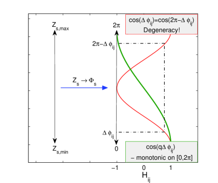
Figure 1: Mapping of continuous data $Z_{s}=\{z_{i}\}_{i=1}^{N}$ where $z_{s,\min}\leq z_{i}\leq z_{s,\max}$, for $i=1,\ldots,N$, to the spin angle set $\Phi_{s}=\{\phi_{i}\}_{i=1}^{N}$, where $0\leq\phi_{i}\leq 2\pi.$ The modified pair interaction $H_{ij}=\cos(q\Delta\phi_{ij})$, with $q=1/2$ (thick green curve) removes the degeneracy of $q=1$ in the standard planar rotator energy $H_{ij}=\cos(\Delta\phi_{ij})$ (thin red curve) and provides a one-to-one mapping $[z_{s,\min},z_{s,\max}]\mapsto[0,2\pi]$.

The sample magentaMPR specific energy of the data is equal to the sample energy per spin pair and is estimated by means of the following sample average

$$e_{s}=-\frac{1}{N_{SP}}\sum_{i=1}^{N}\sum_{j\in nn(i)}\cos[q(\phi_{i}-\phi_{j})],$$ (4)

where $j\in nn(i)$ denotes the sum over the non-missing nearest neighbors of the point $i$, and $N_{SP}$ represents the total number of the nearest-neighbor sample pairs on $G_{s}$.

II.3 Parameter estimation

The two characteristic parameters of the magentaMPR model are the grid size $L$, which is fixed, and the reduced temperature $T$. The latter needs to be estimated from the gappy data in agreement with the sample constraints and the magentaMPR model. We propose a temperature estimation method that is based on matching the sample magentaMPR specific energy defined by (4) with the respective equilibrium magentaMPR specific energy defined by (5) below. We will refer to this estimation method as specific energy matching (SEM).

The equilibrium magentaMPR specific energy is given by

$$e(T,L)=\frac{\langle{\mathcal{H}}\rangle}{N_{GP}},$$ (5)

where $\langle{\mathcal{H}}\rangle$ is the expectation of the magentaMPR energy over all probable states, and $N_{GP}=2L(L-1)$ is the number of nearest-neighbor pairs on the $L\times L$ grid with open boundary conditions. The equilibrium magentaMPR specific energy varies as a function of $L$ and $T$. The expectation $\langle{\mathcal{H}}\rangle$ is numerically evaluated using unconditional simulation of the magentaMPR model as described in Section II.4 below.

The principle of specific energy matching is analogous to the method of moments: assuming ergodic conditions, it posits that $e_{s}=e(\hat{T},L)$, where $e_{s}$ is given by (4), $e(\hat{T},L)$ by (5), and $\hat{T}$ is the characteristic temperature of the gappy sample. If $e(T,L)$ is a known invertible function, so that $e(T,L)=x$, then $T=e^{-1}(x|L)$, where $e^{-1}(\cdot\,|L)$ is the inverse specific energy for fixed $L$. Thus, we can uniquely identify the temperature of the gappy data configuration from $e_{s}$ and $e(T,L)$ by means of $\hat{T}=e^{-1}(e_{s}|L)$.

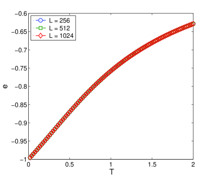
Figure 2: Parametric curves of magentaMPR equilibrium specific energy $e(T,L)$ based on (5) as a function of temperature for three different grid sizes with length per side $L=256,512,1024$. The curves corresponding to the three values of $L$ collapse on each other.

The function $e(T,L)$ is determined by calculating the equilibrium magentaMPR specific energy over any desired domain $[L_{\min},L_{\max}]\times[T_{\min},T_{\max}]$ of the $L$-$T$ parameter plane with some fixed resolution $\Delta L,\Delta T$ that can be further refined by interpolation if needed. As shown in Fig. 2, the specific energy varies smoothly with $T$ and is virtually independent of $L$. Therefore, the curve $e(T,L)$ is calculated once, resulting in a look up table that can be used to estimate the temperature for all magentaMPR applications.

II.4 Hybrid Monte Carlo update algorithm

The estimation of the energy expectation $\langle{\mathcal{H}}\rangle$ involves generating the ensemble of probable states by means of unconditional simulation of the magentaMPR model. The magentaMPR-based gap filling procedure involves the conditional simulation of the magentaMPR model at the estimated temperature $\hat{T}$. Both of these operations require a method for the efficient exploration of the magentaMPR ensemble of states (i.e., the configuration space).

We propose a hybrid Monte Carlo (MC) approach that combines the deterministic over-relaxation (Creutz,, 1987) and the stochastic Metropolis (Metropolis et al.,, 1953) methods (summarized in Algorithm 1). This approach can be used for both conditional and unconditional simulation. The main difference is that the sample set is empty and all the spins can vary in the latter case. This implies significantly longer Monte Carlo sequences for unconditional simulation (typically $10^{6}$ MC sweeps for calculating equilibrium mean values at fixed temperature in addition to approximately $2\times 10^{5}$ MC initial sweeps to reach equilibrium.)

In the initialization phase the sampling locations are assigned the sample-derived values $\Phi_{s}$ that are kept fixed throughout the simulation. The remaining (prediction) locations are first initialized by spins with the set of spin angles $\hat{\Phi}_{p}^{(0)}$, where each angle is in the interval $[0,2\pi]$, and each spin angle value is updated according to the hybrid algorithm. The initial angle assignment is further discussed below.

In the over-relaxation update, new spin angle values are obtained by a simple reflection of the spin about its local molecular field, generated by its nearest neighbors, that conserves the energy. This is accomplished by means of the following transformation

$$\phi^{\prime}_{i}= \,(2\,\Phi_{i}-\phi_{i})\mod{2\pi},$$ (6a)

$$\Phi_{i}= \arctan 2\left(\sum_{j\in nn(i)}\sin{\phi_{j}},\sum_{j\in nn(i)}\cos{\phi_{j}}\right),$$ (6b)

where $nn(i)$ denotes the nearest neighbors of $\phi_{i}$, $i=1,\ldots,N$, and $\arctan 2(\cdot)$ is the four-quadrant inverse tangent: for any $x,y\in\mathbb{R}$ such that $|x|+|y|>0$, $\arctan 2(y,x)$ is the angle (in radians) between the positive horizontal axis and the point $(x,y)$. The over-relaxation transformation reduces autocorrelations, and thus it can significantly speed up the relaxation process (approach to equilibrium). However, since it is energy-conserving and non-ergodic, it has to be mixed with Metropolis updates to achieve ergodicity and explore the probable energy states. In the standard $XY$ model such a hybrid update that uses an optimal ratio of Metropolis and over-relaxation sweeps achieves the correct dynamical critical exponent $z\approx 1.2$, in contrast with $z\approx 2$ for the pure Metropolis algorithm (Gupta et al.,, 1988).

The standard Metropolis local update is rather inefficient, especially at low temperatures: At low $T$ most of the proposed local updates get rejected, implying a very low acceptance ratio $A$ (ratio of accepted updates over the total number of proposed updates). This regime is highly relevant to geostatistical simulations, because the presence of spatial correlations in the data implies a rather low magentaMPR temperature $T$. To increase the efficiency of the relaxation procedure we implement a so-called restricted Metropolis algorithm that generates a proposal spin-angle state according to the rule $\phi^{\prime}=\phi+\alpha(r-0.5)$, where $r$ is a uniformly distributed random number $r\in[0,1)$ and $\alpha=2\pi/a\in(0,2\pi)$ is an adjustable scale factor (tunable parameter). The latter is automatically reset during the equilibration (typically reduced at lower $T$ and increased at higher $T$) to maintain the acceptance ratio $A$ close to a target value $A_{\textrm{targ}}$. Empirically, it is found that $A$ is controlled reasonably well by increasing the perturbation control factor $a$ in linear proportion to the simulation time, when $A$ drops below $A_{\textrm{targ}}$.

The proposed Metropolis state is then accepted or rejected with probability

$$P(\Delta\mathcal{H}_{i})=\min\{1,\exp(-\Delta\mathcal{H}_{i}/T)\},$$

where $\Delta\mathcal{H}_{i}$ is the energy difference between the “new state,” generated by changing the value of the i-th spin angle and the old, i.e.,

$$\Delta\mathcal{H}_{i}=\mathcal{H}_{i}^{\textrm{new}}-\mathcal{H}_{i}^{\textrm{old}}=-\sum_{j\in nn(i)}\{\cos[q(\phi^{\prime}_{i}-\phi_{j})]-\cos[q(\phi_{i}-\phi_{j})]\}.$$

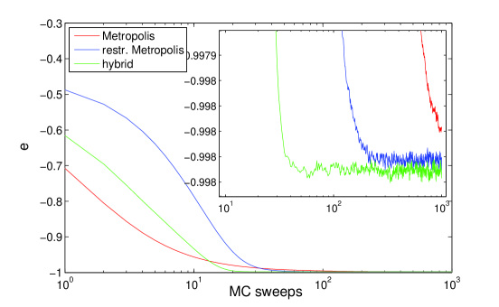
Figure 3: Relaxation process demonstrated by the magentaMPR energy evolution under the application of the standard Metropolis, restricted Metropolis and hybrid (restricted Metropolis combined with over-relaxation) algorithms. Synthetic data are generated by simulating a Gaussian random field with Whittle-Matérn covariance having parameters $\kappa=0.5$ and $\nu=0.5$ on a square grid of size $L=512$ and by randomly removing $p=90\%$ of the data.

The hybrid algorithm combining the restricted Metropolis with over-relaxation dynamics can reduce the magentaMPR relaxation time by several orders of magnitude. Fig. 3 demonstrates the efficiency of the hybrid MC method with respect to standard and restricted Metropolis updates. The synthetic data are simulated from a Gaussian random field with Whittle-Matérn covariance ($\kappa=0.5$ and $\nu=0.5$), on a grid with $L=512$ followed by random removal of $p=90\%$ of the data (see Section IV.1 for details). After an initial phase (up to about $10^{3}$ MC sweeps) of fast relaxation, standard Metropolis significantly slows down due to extremely low acceptance ratio (true equilibrium is not reached even after $10^{6}$ MC sweeps), while hybrid dynamics drives the magentaMPR model to equilibrium after $\approx 50$ MC sweeps. Moreover, our numerical experiments show that the number of hybrid MC sweeps necessary to reach the magentaMPR equilibrium is insensitive to grid size, requiring roughly the same number of MC sweeps for equilibration even for the largest $L$ considered.

In the initial non-equilibrium phase the energy follows a decreasing trend. To automatically detect the crossover to equilibrium (flat regime in the curves of Fig. 3), the energy is periodically evaluated every $n_{f}$ MC sweeps and the variable-degree polynomial Savitzky-Golay (SG) filter is applied (Savitzky and Golay,, 1964). The sampling of equilibrium configurations for the evaluation of ensemble averages (unconditional simulation) or conditional probability distributions (conditional simulation) begins at the point where the trend disappears and the energy shows only fluctuations around a stable level.

Algorithm 1 Hybrid updating algorithm that combines deterministic over-relaxation with the stochastic Metropolis step. $\mathbf{\hat{\Phi}}^{\mathrm{old}}$ is the initial spin state, and $\mathbf{\hat{\Phi}}^{\mathrm{new}}$ is the new spin state. $\mathbf{\hat{\Phi}}^{\mathrm{old}}_{-p}$ is the initial spin state excluding the point labeled by $p$. $U(0,1)$ denotes the uniform probability distribution in $[0,1]$.

procedure Update($\mathbf{\hat{\Phi}}^{\mathrm{new}},\mathbf{\hat{\Phi}}^{\mathrm{old}},a,\hat{T}$)

     for $p=1,\ldots,P$ do $\triangleright$ Loop over prediction sites

         1: ${\hat{\Phi}^{\prime}}_{p}\leftarrow\mathcal{R}\{\hat{\Phi}_{p}^{\mathrm{old}}\}$ $\triangleright$ Over-relaxation step according to (6)

         2: $u\leftarrow U(0,1)$ $\triangleright$ Generate uniform random number

         3: ${\hat{\Phi}^{\prime\prime}}_{p}\leftarrow{\hat{\Phi}^{\prime}}_{p}+2\pi(u-0.5)/a\pmod{2\pi}$ $\triangleright$ Propose spin update

         4: $\Delta\mathcal{H}=\mathcal{H}({\hat{\Phi}^{\prime\prime}}_{p},\mathbf{\hat{\Phi}}^{\mathrm{old}}_{-p})-\mathcal{H}({\hat{\Phi}^{\prime}}_{p},\mathbf{\hat{\Phi}}^{\mathrm{old}}_{-p})$ $\triangleright$ Calculate energy change

         5: $AP=\min\{1,\exp(-\Delta\mathcal{H}/\hat{T})\}$ $\triangleright$ Calculate acceptance probability

         6: $\mathbf{\hat{\Phi}}^{\mathrm{new}}_{-p}\leftarrow\mathbf{\hat{\Phi}}^{\mathrm{old}}_{-p}$ $\triangleright$ Perform Metropolis update

         if $AP>r\leftarrow U(0,1)$ then

              6.1: $\hat{\Phi}_{p}^{\mathrm{new}}\leftarrow{\hat{\Phi}^{\prime\prime}}_{p}$ $\triangleright$ Update the state

         else

              6.2: $\hat{\Phi}_{p}^{\mathrm{new}}\leftarrow{\hat{\Phi}^{\prime}}_{p}$ $\triangleright$ Keep the current state

         end if

     end for$\triangleright$ End of prediction loop

     7: return $\mathbf{\hat{\Phi}}^{\mathrm{new}}$ $\triangleright$ Return the “updated” state

end procedure

II.5 Details of hybrid Monte Carlo magentaMPR simulation

Algorithm 2 Simulation of magentaMPR model. The algorithm involves the hybrid updating procedure Update described in Algorithm 1. $\mathbf{\Phi}_{s}$ is the vector of known spin values at the sample sites. $\mathbf{\hat{\Phi}}$ represents the vector of estimated spin values at the prediction sites. $\hat{T}$ is the estimated reduced temperature. $G(\cdot)$ is the transformation from the original field to the spin field and $G^{-1}(\cdot)$ is its inverse. $\mathbf{\hat{Z}}(j)$, $j=1,\ldots,M$ is the $j$-th realization of the original field. $\mathbf{U}(0,2\pi)$ denotes a vector of random numbers from the uniform probability distribution in $[0,2\pi]$.

1: Initialize simulation parameters

1.1: Set $M$ $\triangleright$ $\#$ equilibrium configurations for statistics collection

1.2: Set $n_{f}$ $\triangleright$ verification frequency of equilibrium conditions

1.3: Set $n_{\textrm{fit}}$ $\triangleright$ $\#$ fitting points of energy evolution function

1.4: Set $A_{\textrm{targ}}$ $\triangleright$ target acceptance ratio of Metropolis update

1.5: Set $k_{a}$ $\triangleright$ defines variation rate of perturbation control factor $a$

1.6: Set $i_{\max}$ $\triangleright$ Monte Carlo relaxation-to-equilibrium steps (optional)

1.7: $i\leftarrow 0$ $\triangleright$ Initialize simulated state counter

1.8: $\mathbf{\hat{\Phi}}(0)\leftarrow\mathbf{U}(0,2\pi)$ $\triangleright$ Initialize missing spin values from uniform distribution

1.9: $k(0)\leftarrow-1$ $\triangleright$ Initialize slope of energy evolution function

1.10: $a(0)\leftarrow 1$ $\triangleright$ Set spin angle perturbation control factor

2: Data transformation

2.1: $\mathbf{\Phi}_{s}\leftarrow G(\mathbf{Z}_{s})$ using (2) $\triangleright$ Set data spin angles

3: Parameter Inference

3.1: Estimate $e_{s}$ using (4) $\triangleright$ Find sample specific energy

3.2: $\hat{T}\leftarrow e^{-1}(e_{s}|L)$ $\triangleright$ Estimate reduced temperature based on $e(\hat{T},L)=e_{s}$

4: Non-equilibrium spin relaxation procedure

while $[k(i)<0]\wedge[i\leq i_{\max}]$  do $\triangleright$ Spin updating with hybrid step

     4.1: Update($\mathbf{\hat{\Phi}}(i+1),\mathbf{\hat{\Phi}}(i),a(i),\hat{T}$)

     if $A<A_{\textrm{targ}}$ then $\triangleright$ Check if Metropolis acceptance ratio is low

         4.2: $a(i+1)\leftarrow 1+(i+1)/k_{a}$ $\triangleright$ Update perturbation control factor

     end if

     4.3: Calculate $e(i+1)\leftarrow\mathcal{H}(G)/N_{GP}$ $\triangleright$ Obtain current specific energy

     if $[i\geq n_{\textrm{fit}}]\wedge[i\equiv 0\pmod{n_{f}}]$ then $\triangleright$ Check frequency for slope update of $e$

         4.4: $k(i+1)\leftarrow\mathrm{SG}$ $\triangleright$ Update slope of $e$ by SG filter using last $n_{\textrm{fit}}$ values

     end if

     4.5: $i\leftarrow i+1$ $\triangleright$ Update MC counter

end while

5. Equilibrium state simulation

5.1: $\mathbf{\hat{\Phi}}^{\mathrm{eq}}(0)\leftarrow\mathbf{\hat{\Phi}}(i)$ $\triangleright$ Initialize the equilibrium state

for $j=0,\ldots,M-1$ do

     5.2: Update($\mathbf{\hat{\Phi}}^{\mathrm{eq}}(j+1),\mathbf{\hat{\Phi}}^{\mathrm{eq}}(j),1,\hat{T}$) $\triangleright$ Generate equilibrium realizations

     5.3: $\mathbf{\hat{Z}}(j+1)\leftarrow G^{-1}\left[\mathbf{\hat{\Phi}}^{\mathrm{eq}}(j+1)\right]$ $\triangleright$ Back-transform spin states

end for

6: return Statistics of $M$ realizations $\mathbf{\hat{Z}}(j),\,j=1,\ldots,M$

Algorithm 2 summarizes the main steps of the magentaMPR method for conditional simulation of gappy data. To avoid undesirable boundary effects, we add auxiliary nodes around the grid that are assigned the same values as their nearest grid neighbors. The augmented grid is used with open boundary conditions. Therefore, if ${\mathbf{s}}_{i,j}$ is a spin in the $i$-th row and $j$-th column of the grid, where $i,j=1,\dots,L$, then ${\mathbf{s}}_{i,L+1}={\mathbf{s}}_{i,L}$, ${\mathbf{s}}_{L+1,j}={\mathbf{s}}_{L,j}$, ${\mathbf{s}}_{i,0}={\mathbf{s}}_{i,1}$ and ${\mathbf{s}}_{0,j}={\mathbf{s}}_{1,j}$, where the indices $0$ and $L+1$ refer to auxiliary nodes.

Algorithm 2 involves several control factors that include: the number of equilibrium configurations for collecting statistics, $M$, the frequency of verification of equilibrium conditions, $n_{f}$, the number of points used for fitting the energy evolution function, $n_{\textrm{fit}}$, the maximum number of Monte Carlo steps $i_{\max}$ (optional), and the parameters $A_{\textrm{targ}}$ and $k_{a}$ used in the restricted Metropolis update. Below, we comment on the selection of these factors and their impact on prediction performance.

• $M$ is set arbitrarily, depending on whether the main goal is computational efficiency or prediction performance. Lower (higher) values of $M$ increase (decrease) the computational speed and decrease (increase) accuracy and precision. For the conditional simulations we set $M=100$.

• High-frequency checking of equilibrium conditions (small $n_{f}$) slightly slows down the simulation but can also lead to earlier onset of equilibrium calculations. A reasonable value of $n_{f}$ is determined based on the maximum total equilibration time. In conditional simulation the latter is about 50 MCS and $n_{f}=5$ in all cases.

• The parameter $n_{\textrm{fit}}$ defines the memory length of the energy time series used to test the onset of equilibrium. Close to equilibrium, where fluctuations can be considerable, $n_{\textrm{fit}}$ should be sufficiently large to ensure a robust fit (i.e., to distinguish the fluctuations from the trend). We found empirically that $n_{\textrm{fit}}=20$ is adequate for this purpose.

• The factor $i_{\max}$ prevents very long equilibration times, if the convergence is very slow. Since the employed hybrid algorithm leads to very fast equilibration, the value of $i_{\max}$ is practically irrelevant.

• We tested several initialization approaches for the spin angle state, including uniform and random assignments that correspond respectively to the “ferromagnetic” (cold start) and “paramagnetic” (hot start) initializations, typically used in spin system simulations. In conditional simulation we also tried configurations obtained by simple and fast interpolation of the sample data, e.g., nearest neighbors and bilinear methods. Since different initializations did not produce significant differences, we use the “paramagnetic” state as default with random values drawn from the uniform distribution in $[0,2\pi]$.

• The adjustable scale parameters $A_{\textrm{targ}}$ and $k_{a}$ are introduced to avoid low-temperature inefficiency due to the Metropolis acceptance ratio dropping to low values. Since their actual values appear to have little influence on the prediction performance, we arbitrarily set them to $A_{\textrm{targ}}=0.3$ and $k_{a}=3$.

In conclusion, the effect of the Monte Carlo simulation control factors on prediction performance is marginal. Thus, the default values set above can be safely used in general. Combined with the fact that the temperature estimation is straightforward and does not require parameter tuning, this means that the magentaMPR conditional simulation method can be automatically applied without user intervention.

III Design of MPR-Prediction Validation and Comparison

The magentaMPR model and Algorithms 1-2 provide a framework for fast conditional simulation. The magentaMPR predictions are based on the conditional mean as evaluated from the conditionally simulated reconstructions. We assess the magentaMPR performance as a gap-filling method by comparison with established interpolation methods using both synthetic and real data. We simulate missing values by setting aside a portion of the complete data to use as validation set.

The magentaMPR comparison with interpolation methods is implemented in the Matlab® environment running on a desktop computer with 16.0 GB RAM and an Intel®Core™2 i7-4790 CPU processor with an 3.60 GHz clock. The methods tested involve the triangulation-based nearest neighbor (NN), bilinear (BL) and bicubic (BC) interpolation using the built-in function griddata, as well as the minimum curvature (MC) (or biharmonic spline) method (Sandwell,, 1987). We also include the deterministic inverse distance weighted (IDW) (Shepard,, 1968) interpolation, using the Matlab®  function fillnans (Howat,, 2007), and the stochastic ordinary kriging (OK) method (Wackernagel,, 2003), using the routines available in the Matlab®  library vebyk (Sidler,, 2003). We note that a number of functions useful in spatial and spatio-temporal geostatistical modelling can be also found in the freely distributed R programming environment, such as the package gstat (Pebesma,, 2004; Pebesma et al.,, 2016). The IDW, MC and OK methods are applied using the entire sample data set (without search neighborhoods). OK is applied to the Gaussian data using the “true” covariance parameters. Thus, it provides optimal predictions that serve as a standard for comparison with the magentaMPR estimates. The above spatial interpolation methods are commonly used in the environmental sciences (Li and Heap,, 2014).

We employ several validation measures for performance comparison. Let $Z(\mathbf{r}_{p})$ be the true value at $\mathbf{r}_{p}$ and $\hat{Z}(\mathbf{r}_{p})$ its estimated value. The estimation error is defined as $\epsilon(\mathbf{r}_{p})=Z(\mathbf{r}_{p})-\hat{Z}(\mathbf{r}_{p})$. The following validation measures are then defined:

Average absolute error

$${\rm AAE}=(1/P)\sum_{\mathbf{r}_{p}\in G_{p}}|\epsilon(\mathbf{r}_{p})|$$ (7)

Average relative error

$${\rm ARE}=(1/P)\sum_{\mathbf{r}_{p}\in G_{p}}\epsilon(\mathbf{r}_{p})/Z(\mathbf{r}_{p})$$ (8)

Average absolute relative error

$${\rm AARE}=(1/P)\sum_{\mathbf{r}_{p}\in G_{p}}|\epsilon(\mathbf{r}_{p})|/Z(\mathbf{r}_{p})$$ (9)

Root average squared error

$${\rm RASE}=\sqrt{\frac{1}{P}\sum_{\mathbf{r}_{p}\in G_{p}}\,\epsilon^{2}(\mathbf{r}_{p})}.$$ (10)

The above are complemented by the linear correlation coefficient $R$. Furthermore, for each method we record the required CPU time, $t_{\mathrm{cpu}}$. For each complete data set we generate $S$ different sample configurations with missing data and calculate the above validation measures. Global statistics, denoted by MAAE, MARE, MAARE, MRASE, MR and $\langle t_{\mathrm{cpu}}\rangle$, are then calculated by averaging over all the sample configurations.

IV Gap-filling Validation Results

IV.1 Synthetic data

Synthetic data are simulated on the square grid from the Gaussian random field $Z\sim N(m=50,\sigma=10)$ with Whittle-Matérn (WM) covariance given by

$$G_{\rm Z}(\|\mathbf{h}\|)=\frac{{2}^{1-\nu}\,\sigma^{2}}{\Gamma(\nu)}(\kappa\,\|\mathbf{h}\|)^{\nu}K_{\nu}(\kappa\,\|\mathbf{h}\|),$$ (11)

where $\|\mathbf{h}\|$ is the Euclidean two-point distance, $\sigma^{2}$ is the variance, $\nu$ is the smoothness parameter, $\kappa$ is the inverse autocorrelation length, and $K_{\nu}$ is the modified Bessel function of index $\nu$. Hereafter, only the parameters $\kappa$ and $\nu$ will change. For such data we use the abbreviation WM($\kappa,\nu)$. The field is sampled on a square grid $G$ using the spectral method (Drummond and Horgan,, 1987). Incomplete samples ${Z}(G_{s})$ of size $N=N_{G}-\lfloor(p/100\%)\,N_{G}\rfloor$ are generated by removing (i) randomly $P=\lfloor(p/100\%)\,N_{G}\rfloor$ points or (ii) a randomly selected solid square block of side length $L_{B}$. For different degrees of thinning ($p=33\%$ and $66\%$) and block size ($L_{B}=5$ and $20$), we generate $S=100$ different sampling configurations. The predictions at the removed (validation) points are calculated and compared with the true values.

The WM family is flexible and includes several variogram models (Minasny and McBratney,, 2005; Pardo-Igúzquiza and Chica-Olmo,, 2008; Pardo-Igúzquiza et al.,, 2009). Small values of $\nu$, e.g., $\nu=1/2$, which is equivalent to the exponential model, imply that the spatial process is rough. On the other hand, large values, e.g., $\nu\to\infty$, which is equivalent to the Gaussian model, generate smooth processes. In our simulations we use $\nu=0.25-0.5$, which is appropriate for modeling rough spatial processes such as soil data (Minasny and McBratney,, 2005).

Table 1: Interpolation validation measures for the magentaMPR method and relative values, ${\rm XX^{*}=\textcolor{magenta}{MPR}/XX}$, for all other methods. $S=100$ samples are generated from a Gaussian random field with mean equal to 50 on a square grid with side length $L=16$. Two covariance models, WM($\kappa=0.5,\nu=0.5$) and WM($\kappa=0.5,\nu=0.25$) are used. Missing data are generated by (a) $p=33\%$ (b) $p=66\%$ random thinning and (c) random removal of square data block with side length $L_{B}=5$. Boldfaced values denote that the respective method performs better than magentaMPR for the specific validation measure.

		MAAE			MARE [%]			MAARE [%]			MRASE			MR [%]			$\langle t_{\mathrm{cpu}}\rangle$
$\nu$		(a)	(b)	(c)	(a)	(b)	(c)	(a)	(b)	(c)	(a)	(b)	(c)	(a)	(b)	(c)	(a)	(b)	(c)
	magentaMPR	5.17	5.92	6.38	$-$1.89	$-$2.37	$-$0.10	11.11	12.75	12.70	6.56	7.47	7.89	73.01	63.90	37.62	0.01	0.02	0.01
	${\rm NN^{*}}$	0.75	0.81	0.80	1.26	1.13	$-$0.39	0.76	0.82	0.81	0.76	1.16	0.80	1.23	1.16	1.26	10.63	15.69	7.89
	${\rm BL^{*}}$	0.94	0.98	0.88	1.37	2.08	$-$0.21	0.96	1.01	0.89	0.96	0.99	0.89	1.23	1.17	1.25	8.00	14.08	5.45
$0.5$	${\rm BC^{*}}$	0.95	0.97	0.86	1.29	1.56	$-$0.27	0.96	1.00	0.87	0.96	0.98	0.87	1.02	1.00	1.35	12.99	21.40	8.83
	${\rm MC^{*}}$	0.96	0.97	0.93	1.62	1.65	0.08	0.96	0.98	0.93	0.97	0.96	0.93	1.00	0.97	1.01	3.36	6.74	2.13
	${\rm IDW^{*}}$	0.99	1.01	0.99	0.82	0.93	0.26	0.99	1.01	0.99	0.99	1.00	0.99	1.01	0.99	0.96	4.49	5.23	7.50
	${\rm OK^{*}}$	1.04	1.05	1.03	1.00	0.99	1.06	1.04	1.04	1.03	1.04	1.05	1.03	0.97	0.94	0.89	1e$-$4	5e$-$4	5e$-$5
	magentaMPR	7.04	7.63	7.90	$-$3.19	$-$3.60	$-$3.90	15.21	16.62	17.12	8.75	9.44	9.59	47.87	36.69	29.77	0.01	0.02	0.01
	${\rm NN^{*}}$	0.78	0.81	0.78	1.01	1.02	1.02	0.79	0.82	0.80	0.78	0.81	0.79	1.37	1.17	1.43	10.99	15.92	7.45
	${\rm BL^{*}}$	0.96	0.96	0.89	1.16	1.11	0.85	0.97	0.97	0.89	0.95	0.96	0.89	1.35	1.13	1.40	8.29	14.04	5.13
$0.25$	${\rm BC^{*}}$	0.94	0.94	0.87	1.18	1.12	0.88	0.95	0.95	0.87	0.93	0.93	0.86	1.04	1.00	1.58	13.33	21.23	8.52
	${\rm MC^{*}}$	0.94	0.92	0.88	1.20	1.07	1.18	0.94	0.92	0.89	0.93	0.91	0.88	0.99	0.97	1.08	3.44	6.66	2.01
	${\rm IDW^{*}}$	1.01	0.99	0.98	0.98	1.00	0.88	1.01	0.99	0.98	1.01	0.99	0.98	0.98	0.95	0.98	4.54	5.27	6.70
	${\rm OK^{*}}$	1.01	1.02	1.01	0.94	0.91	0.88	1.00	1.01	1.01	1.02	1.03	1.02	0.97	0.92	0.91	1e$-$4	5e$-$4	4e$-$5

IV.1.1 Small grid size

In Table 1 we present the magentaMPR interpolation validation measures for the smallest ($L=16$) grid size using an autocorrelation length $1/\kappa=2$. For this data size we compare the performance of the magentaMPR model with all the methods presented above, including the optimal but computationally intensive OK method. The actual values of the validation measures are shown only for the magentaMPR method. For other methods XX (= NN, BL, BC, MC, IDW, OK) the validation measures are expressed relative to the magentaMPR method, i.e., ${\rm XX^{*}=\textcolor{magenta}{MPR}/XX}$. Therefore, MAAE, MARE, MAARE, MRASE and $\langle t_{\mathrm{cpu}}\rangle$ less than one and correlation coefficient values higher than one indicate superior performance of magentaMPR. Boldfaced values denote that the respective method performs better than magentaMPR with respect to the specific validation measure or $\langle t_{\mathrm{cpu}}\rangle$.

The magentaMPR method performs better than the NN, BL and BC methods in terms of most measures, except for the MARE errors in the case of randomly thinned data and the CPU time. The relative “slowness” of magentaMPR is due to the fact that the method performs conditional simulation (hence, it generates considerably more information than an “optimal” prediction). The MC method returns better MARE while its MR is comparable with the magentaMPR method. Even better results are obtained with IDW, albeit still slightly worse than the magentaMPR (except for the MR indicator and the CPU time). Comparing the magentaMPR and OK methods, OK is optimal with respect to all the measures except for the MARE errors and the CPU time. The superior prediction performance of OK is not surprising, considering that it is the optimal model for Gaussian data with known covariance parameters. On the other hand, if a search neighborhood is not specified, the CPU time required by OK exceeds that of magentaMPR by about four orders of magnitude.

IV.1.2 Larger grids

Table 2: Interpolation validation measures for the magentaMPR method and relative values, ${\rm XX^{*}=\textcolor{magenta}{MPR}/XX}$, for the other methods except OK. $S=100$ samples are generated from a Gaussian random field with mean equal to 50 on a square grid with side length $L=32,64,128$. The covariance model WM($\kappa=0.2,\nu=0.5$) is used. Missing data are generated by (a) $p=33\%$ (b) $p=66\%$ random thinning and (c) random removal of square data block with side length $L_{B}=20$. Boldfaced values denote that the respective method performs better than magentaMPR for the specific validation measure.

		MAAE			MARE [%]			MAARE [%]			MRASE			MR [%]			$\langle t_{\mathrm{cpu}}\rangle$
$L$		(a)	(b)	(c)	(a)	(b)	(c)	(a)	(b)	(c)	(a)	(b)	(c)	(a)	(b)	(c)	(a)	(b)	(c)
	magentaMPR	3.48	4.03	6.95	$-$1.08	$-$1.46	$-$4.64	7.41	8.70	16.12	4.36	5.10	8.98	90.66	87.12	45.73	0.02	0.04	0.03
	${\rm NN^{*}}$	0.70	0.77	0.79	1.48	1.82	1.02	0.70	0.78	0.81	0.70	0.78	0.79	1.11	1.10	1.30	9.47	17.67	7.72
	${\rm BL^{*}}$	0.95	0.97	0.85	1.14	1.07	0.86	0.95	0.98	0.85	0.95	0.97	0.87	1.11	1.09	1.27	5.31	12.71	6.46
$32$	${\rm BC^{*}}$	0.96	0.98	0.84	1.57	1.45	0.93	0.97	1.00	0.85	0.96	0.98	0.86	1.01	1.01	1.29	10.05	23.06	12.20
	${\rm MC^{*}}$	1.01	1.02	0.90	1.88	1.90	2.59	1.03	1.04	0.94	1.00	1.02	0.91	1.00	1.00	1.00	0.59	1.72	0.74
	${\rm IDW^{*}}$	0.97	0.98	1.00	0.89	1.17	0.75	0.96	0.98	0.99	0.97	0.98	1.00	1.01	1.01	0.94	0.69	1.11	0.73
	magentaMPR	3.38	3.86	6.69	$-$0.92	$-$1.28	$-$3.29	7.13	8.16	14.55	4.27	4.89	8.42	89.38	85.92	49.09	0.07	0.13	0.03
	${\rm NN^{*}}$	0.70	0.77	0.84	1.43	1.62	1.18	0.71	0.78	0.85	0.70	0.78	0.83	1.12	1.10	1.21	8.30	17.55	2.99
	${\rm BL^{*}}$	0.94	0.97	0.88	1.09	1.17	0.96	0.94	0.97	0.88	0.94	0.97	0.88	1.13	1.10	1.21	4.14	11.39	1.45
$64$	${\rm BC^{*}}$	0.94	0.97	0.86	1.34	1.43	1.04	0.95	0.98	0.87	0.95	0.97	0.87	1.01	1.01	1.36	8.40	22.79	2.98
	${\rm MC^{*}}$	0.98	0.99	0.90	1.61	1.70	1.47	0.99	1.00	0.92	0.98	1.00	0.89	1.00	1.00	1.04	0.09	0.36	0.02
	${\rm IDW^{*}}$	0.97	0.97	0.98	0.88	1.12	0.94	0.97	0.98	0.98	0.97	0.98	0.98	1.01	1.01	1.08	0.20	0.25	0.27
	magentaMPR	3.45	3.89	6.21	$-$1.05	$-$1.36	$-$3.89	7.37	8.34	13.75	4.34	4.90	7.86	90.50	87.71	55.40	0.27	0.49	0.05
	${\rm NN^{*}}$	0.71	0.77	0.82	1.27	1.47	1.38	0.71	0.78	0.85	0.71	0.77	0.81	1.10	1.09	1.24	6.95	14.94	1.08
	${\rm BL^{*}}$	0.94	0.97	0.87	1.08	1.15	1.15	0.94	0.97	0.89	0.94	0.97	0.88	1.10	1.09	1.24	3.43	9.54	0.44
$128$	${\rm BC^{*}}$	0.94	0.96	0.86	1.28	1.37	1.16	0.95	0.97	0.87	0.94	0.96	0.87	1.01	1.01	1.31	6.94	18.79	0.95
	${\rm MC^{*}}$	0.98	0.98	0.85	1.51	1.65	1.06	0.99	0.99	0.88	0.98	0.98	0.86	1.00	1.00	1.10	0.01	0.07	8e$-$4
	${\rm IDW^{*}}$	0.97	0.97	0.98	0.89	1.08	1.12	0.97	0.98	0.98	0.97	0.97	0.98	1.01	1.01	1.04	0.08	0.15	0.08

Table 3: Interpolation validation measures for the magentaMPR method and relative values, ${\rm XX^{*}=\textcolor{magenta}{MPR}/XX}$, for the other methods except OK. $S=100$ samples are generated from a Gaussian random field with mean equal to 50 on a square grid with side length $L=32,64,128$. The covariance model WM($\kappa=0.2,\nu=0.25$) is used. Missing data are generated by (a) $p=33\%$ (b) $p=66\%$ random thinning and (c) random removal of square data block with side length $L_{B}=20$. Boldfaced values denote that the respective method performs better than magentaMPR for the specific validation measure.

		MAAE			MARE [%]			MAARE [%]			MRASE			MR [%]			$\langle t_{\mathrm{cpu}}\rangle$
$L$		(a)	(b)	(c)	(a)	(b)	(c)	(a)	(b)	(c)	(a)	(b)	(c)	(a)	(b)	(c)	(a)	(b)	(c)
	magentaMPR	5.50	5.81	6.62	$-$1.74	$-$1.90	$-$2.32	11.54	12.19	13.70	6.86	7.32	8.34	65.93	59.84	31.26	0.02	0.04	0.03
	${\rm NN^{*}}$	0.76	0.79	0.75	1.21	1.35	1.84	0.77	0.80	0.76	0.77	0.80	0.75	1.28	1.23	1.48	9.59	17.94	7.60
	${\rm BL^{*}}$	0.93	0.94	0.82	0.88	0.95	1.75	0.93	0.94	0.83	0.93	0.94	0.82	1.28	1.22	1.43	5.40	12.79	6.42
$32$	${\rm BC^{*}}$	0.91	0.91	0.78	0.99	1.09	1.68	0.91	0.91	0.80	0.91	0.92	0.79	1.08	1.07	1.74	10.29	23.45	12.19
	${\rm MC^{*}}$	0.92	0.90	0.66	1.19	1.27	1.19	0.93	0.91	0.67	0.92	0.91	0.68	1.05	1.06	1.29	0.60	1.78	0.75
	${\rm IDW^{*}}$	1.00	0.97	0.99	0.95	1.07	2.45	1.00	0.98	1.01	1.00	0.98	0.99	1.00	1.02	1.01	0.71	1.13	0.74
	magentaMPR	5.53	5.88	7.18	$-$2.24	$-$2.51	$-$4.11	11.88	12.69	0.16	6.94	7.41	9.05	72.02	67.21	36.33	0.07	0.13	0.03
	${\rm NN^{*}}$	0.75	0.79	0.78	1.17	1.23	1.06	0.76	0.80	0.79	0.75	0.79	0.78	1.25	1.21	1.32	8.29	17.64	3.01
	${\rm BL^{*}}$	0.93	0.94	0.87	1.03	1.08	1.07	0.93	0.95	0.88	0.93	0.94	0.87	1.25	1.21	1.32	4.13	11.39	1.46
$64$	${\rm BC^{*}}$	0.91	0.91	0.83	1.12	1.16	1.14	0.92	0.93	0.85	0.91	0.91	0.84	1.07	1.07	1.51	8.38	22.89	2.99
	${\rm MC^{*}}$	0.93	0.91	0.73	1.20	1.19	1.49	0.94	0.92	0.75	0.92	0.91	0.74	1.04	1.05	1.32	0.09	0.36	0.02
	${\rm IDW^{*}}$	1.00	0.97	0.99	0.95	1.06	0.84	0.99	0.98	0.99	1.00	0.97	1.00	1.00	1.02	1.01	0.20	0.25	0.27
	magentaMPR	5.53	5.84	7.32	$-$2.11	$-$2.43	$-$3.18	11.85	12.58	15.87	6.92	7.31	9.16	74.04	70.40	39.38	0.28	0.50	0.05
	${\rm NN^{*}}$	0.76	0.78	0.78	1.15	1.21	1.26	0.77	0.79	0.80	0.76	0.78	0.78	1.22	1.20	1.39	7.29	15.39	1.10
	${\rm BL^{*}}$	0.93	0.94	0.86	1.05	1.08	1.14	0.93	0.94	0.87	0.93	0.94	0.87	1.22	1.20	1.39	3.47	9.73	0.45
$128$	${\rm BC^{*}}$	0.90	0.91	0.83	1.13	1.16	1.19	0.91	0.92	0.84	0.90	0.91	0.83	1.06	1.07	1.62	7.04	19.34	0.96
	${\rm MC^{*}}$	0.92	0.91	0.77	1.20	1.23	0.88	0.93	0.92	0.79	0.92	0.90	0.78	1.04	1.06	1.28	0.01	0.07	8e$-$4
	${\rm IDW^{*}}$	1.00	0.97	0.99	0.95	1.04	1.06	1.00	0.97	0.99	1.00	0.97	0.99	1.00	1.02	1.00	0.08	0.15	0.09

Table 4: Interpolation validation measures for the magentaMPR method. $S=100$ samples are generated from a Gaussian random field with mean equal to 50 on a square grid with side length $L=2^{n}$, where $n=8,9,10,11$. Two covariance models, WM($\kappa=0.2,\nu=0.5$) and WM($\kappa=0.2,\nu=0.25$) are used. Missing data are generated by (a) $p=33\%$ (b) $p=66\%$ random thinning and (c) random removal of square data block with side length $L_{B}=20$.

		MAAE			MARE [%]			MAARE [%]			MRASE			MR [%]			$\langle t_{\mathrm{cpu}}\rangle$
$\nu$	$L$	(a)	(b)	(c)	(a)	(b)	(c)	(a)	(b)	(c)	(a)	(b)	(c)	(a)	(b)	(c)	(a)	(b)	(c)
	$256$	3.39	3.83	6.33	$-$0.98	$-$1.29	$-$3.34	7.19	8.16	14.02	4.26	4.84	7.95	90.47	87.62	52.90	0.89	1.58	0.10
0.5	$512$	3.38	3.83	6.27	$-$0.98	$-$1.29	$-$2.41	7.16	8.16	13.29	4.24	4.83	7.91	90.49	87.55	54.36	3.47	6.71	0.51
	$1024$	3.38	3.83	6.34	$-$0.99	$-$1.30	$-$3.78	7.17	8.16	13.87	4.24	4.82	7.99	90.70	87.89	54.52	19.47	35.83	2.24
	$2048$	3.38	3.83	6.32	$-$0.99	$-$1.29	$-$2.86	7.17	8.15	13.71	4.24	4.82	7.98	90.59	87.74	52.41	85.83	149.11	9.12
.	$256$	5.51	5.82	7.20	$-$2.10	$-$2.39	$-$4.19	11.79	12.51	15.90	6.92	7.31	9.01	72.24	68.23	36.05	0.88	1.55	0.11
0.25	$512$	5.50	5.80	7.39	$-$2.09	$-$2.39	$-$3.56	11.77	12.45	16.18	6.90	7.27	9.28	72.69	68.87	36.32	3.59	6.42	0.51
	$1024$	5.48	5.79	7.25	$-$2.08	$-$2.38	$-$5.06	11.72	12.42	16.03	6.87	7.26	9.06	72.88	69.02	36.34	20.08	36.50	2.40
	$2048$	5.48	5.78	7.17	$-$2.08	$-$2.37	$-$3.76	11.71	12.40	15.50	6.87	7.25	8.97	72.70	68.83	36.08	85.04	148.77	9.28

For larger data sizes, we exclude the OK method from the comparison due to its high computational cost. In Tables 2 and 3 we present similar comparisons as those in Table 1, for square grids with side lengths $L=32,64$ and $128$. As $L$ increases, the relative performance of the magentaMPR method improves (except for the MARE errors). Thus, for $L=64$ and $128$, the magentaMPR approach is superior to NN, BL, BC, MC and IDW methods in terms of validation measures (except MARE). magentaMPR also has significantly shorter CPU times than MC and IDW. The lower MARE of the magentaMPR method is due to a less symmetric error distribution.

Finally, we study the performance of the magentaMPR method on increasing grid sizes $L=2^{n}$ where $n=8,9,10,11$. The results are summarized in Table 4. Increasing $L$ does not impact the validation measures. However, a closer look reveals a small but noticeable improving trend (more apparent for $\nu=0.25$), in agreement with the trend observed in Tables 2 and 3. On the other hand, the CPU time increases drastically with $L$. Nevertheless, the scaling of the magentaMPR CPU time with $L$ is competitive with the alternative approaches, as we discuss in more detail below.

IV.1.3 Single sample statistics

(a) Original

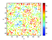
(b) $p=66\%$ missing

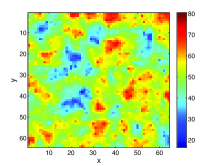
(c) Interpolated

(d) Standard deviation

(e) Interpolation error

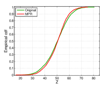
(f) Empirical cdf

Figure 4: magentaMPR interpolation results for WM($\kappa=0.2,\nu=0.5$), with $L=64$, generated by $p=66\%$ random thinning. Subfigures include (a) original field, (b) thinned sample, (c) interpolated data, (d) local standard deviation $\sigma(\mathbf{r}_{p})$, (e) local estimation error $\epsilon(\mathbf{r}_{p})$, and (f) comparison of the empirical cumulative distribution functions of the original and interpolated data.

In Fig. 4 we investigate the prediction performance of the magentaMPR model based on a single synthetic sample. The sample is generated by simulating a random field with WM($\kappa=0.2,\nu=0.5$) covariance model on a square grid of size $L=64$. Then, $p=66\%$ of the field values are randomly removed to generate the sample. Panels (a) and (b) show the simulated random field realization and the sample obtained after random thinning, respectively. The remaining panels illustrate the prediction performance in terms of (c) the interpolated data over the entire grid (d) the standard deviation and (e) the interpolation error $\epsilon(\mathbf{r}_{p})$ at the missing points, as well as (f) the empirical cumulative distribution functions of the original and the interpolated data. It is evident that the magentaMPR predictor fairly accurately reconstructs basic statistical features of the original data. On the other hand, panels (c) and (f) provide evidence that the interpolated field is overly smooth. The issue of over-smoothing and the ability of magentaMPR to capture the spatial data variability will be discussed more below in the context of block-missing real data.

IV.2 Real data

IV.2.1 Data descriptive statistics

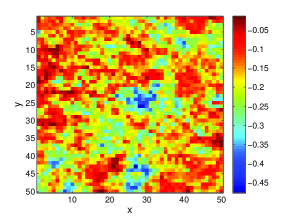
(a) Latent heat map

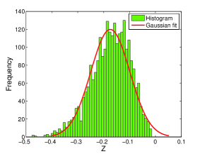
(b) Latent heat histogram

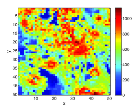
(c) Walker lake map

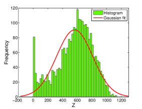
(d) Walker lake histogram

Figure 5: (a,b) Latent heat and (c,d) Walker lake data maps and histograms.

We assess the performance of magentaMPR prediction by means of two real-world environmental data sets that follow non-Gaussian distributions. The first set represents the monthly mean of vertically averaged atmospheric latent heat release measurements in January 2006 (Tao et al.,, 2006; TRMM,, 2011). The data are on an $L=50$ grid with a $0.5^{\circ}\times 0.5^{\circ}$ cell size, extending in latitude from 16S to 8.5N and in longitude from 126.5E to 151E. The measurement units are C/hr (degrees Celsius per hour), and their summary statistics are as follows: $N=2500$, $z_{\min}=-0.4772$, $z_{\max}=-0.0141$, $\bar{z}=-0.1743$, $z_{0.50}=-0.1680$, $\sigma_{z}=0.0755$, skewness coefficient equal to $-0.5153$, and kurtosis coefficient equal to $3.1218$. Negative (positive) values correspond to latent heat absorption (release).

The second example is a subset of the DEM-based data from Walker lake area in Nevada (Isaak and Srivastava,, 1989). The data denote chemical concentrations with units in parts per million (ppm). They are sampled on an $L=50$ grid, and they exhibit the following summary statistics: $N=2500$, $z_{\min}=0$, $z_{\max}=1138.6$, $\bar{z}=564.1435$, $z_{0.50}=601.0950$, $\sigma_{z}=245.7724$, skewness coefficient equal to $-0.5295$, and kurtosis coefficient equal to $2.7351$.

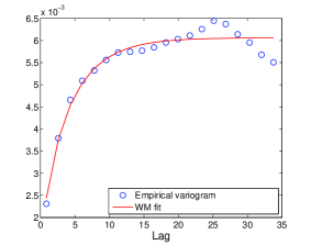
(a) Latent heat variogram

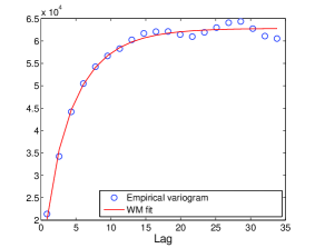
(b) Walker lake variogram

Figure 6: Empirical (circles) and fitted (solid line) variograms of (a) latent heat and (b) Walker lake data. The estimated parameters of the WM variogram model are as follows: (a) $\sigma=0.07$, $\kappa=0.21$, and $\nu=0.34$; (b) $\sigma=250.62$, $\kappa=0.18$, and $\nu=0.29$.

Surface and histogram plots for both data sets are shown in Fig. 5. The histograms clearly show the deviations from the Gaussian distribution. Fig. 6 presents the empirical variograms and their respective fits with the WM model using the weighted least squares method (Cressie,, 1985). The estimated parameter values indicate that both data sets are examples of relatively rough spatial processes ($\nu=0.34$ and $\nu=0.29$ respectively), with similar spatial variability to the synthetic data.

IV.2.2 Gap-filling performance

The magentaMPR prediction performance evaluation is summarized for both data sets and different patterns of missing data in Table 5. Due to the presence of negative and zero values, the relative errors MARE and MAARE are excluded from the comparison. Table 5 shows that in terms of prediction accuracy the magentaMPR method is superior to all other methods (NN, BL, BC, IDW, MC), except for a few cases where IDW performs slightly better (cf. bold figures in the MAAE and MRASE columns). In terms of computational time, magentaMPR is more efficient than MC and IDW but less efficient than NN, BL and BC (cf. bold figures in the $\langle t_{\mathrm{cpu}}\rangle$ column).

In Figs. 7 and 8 we present examples of interpolated maps for different patterns of missing data, using three methods that give the best prediction performance, i.e., the magentaMPR, IDW and MC. For randomly thinned data, visual differences between predictions obtained by individual methods are not so obvious. All methods display smoothing that naturally increases with the fraction of missing data. The biggest differences between the methods appear in the case of missing solid data blocks.

Table 5: Interpolation validation measures for real data based on $S=100$ missing-data samples generated by (a) $p=33\%$, (b) $p=66\%$ random thinning and (c) random removal of square data block with side length $L_{B}=20$.

		MAAE			MRASE			MR [%]			$\langle t_{\mathrm{cpu}}\rangle$
Data set		(a)	(b)	(c)	(a)	(b)	(c)	(a)	(b)	(c)	(a)	(b)	(c)
Latent heat	magentaMPR	0.04	0.04	0.06	0.05	0.05	0.07	79.25	72.40	38.14	0.05	0.09	0.03
	${\rm NN^{*}}$	0.72	0.80	0.80	0.71	0.79	0.78	1.25	1.17	1.35	9.01	18.82	4.31
	${\rm BL^{*}}$	0.95	0.96	0.87	0.94	0.95	0.87	1.25	1.16	1.36	4.59	12.35	2.33
	${\rm BC^{*}}$	0.95	0.95	0.85	0.94	0.94	0.84	1.03	1.04	1.57	9.28	24.85	4.79
	${\rm MC^{*}}$	1.00	0.97	0.81	0.99	0.96	0.80	1.00	1.01	1.21	0.18	0.65	0.08
	${\rm IDW^{*}}$	0.98	1.00	1.02	0.98	0.99	1.01	1.01	1.01	1.01	0.25	0.43	0.40
Walker lake	magentaMPR	102.02	117.52	167.93	138.97	156.57	212.55	82.79	77.51	45.32	0.05	0.09	0.03
	${\rm NN^{*}}$	0.76	0.85	0.83	0.73	0.80	0.80	1.17	1.14	1.27	9.00	18.79	4.32
	${\rm BL^{*}}$	0.96	0.99	0.91	0.93	0.96	0.88	1.17	1.14	1.27	4.59	12.43	2.35
	${\rm BC^{*}}$	0.96	0.98	0.89	0.93	0.94	0.86	1.03	1.04	1.33	9.24	24.71	4.82
	${\rm MC^{*}}$	0.99	0.98	0.76	0.97	0.95	0.75	1.01	1.02	1.24	0.18	0.63	0.08
	${\rm IDW^{*}}$	0.98	1.01	1.00	0.98	0.99	0.99	1.01	1.01	1.02	0.25	0.43	0.41

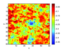
(a) magentaMPR, $p=33\%$

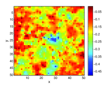
(b) magentaMPR, $p=66\%$

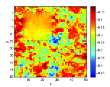
(c) magentaMPR, $L_{B}=20$

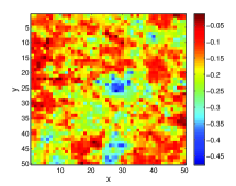
(d) IDW, $p=33\%$

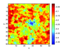
(e) IDW, $p=66\%$

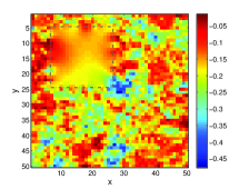
(f) IDW, $L_{B}=20$

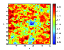
(g) MC, $p=33\%$

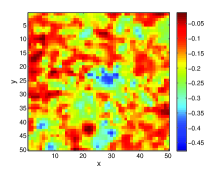
(h) MC, $p=66\%$

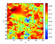
(i) MC, $L_{B}=20$

Figure 7: Visual comparison of magentaMPR, IDW and MC interpolated maps for the latent heat data shown in Fig. 5(a). Three different patterns of missing data are used: 33% random thinning (left column), 66% random thinning (middle column) and solid block removal (right column). The perimeter of the missing data block is marked by the dashed line.

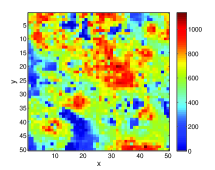
(a) magentaMPR, $p=33\%$

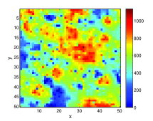
(b) magentaMPR, $p=66\%$

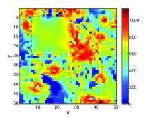
(c) magentaMPR, $L_{B}=20$

(d) IDW, $p=33\%$

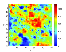
(e) IDW, $p=66\%$

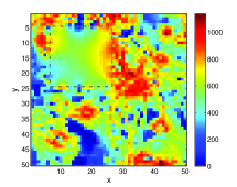
(f) IDW, $L_{B}=20$

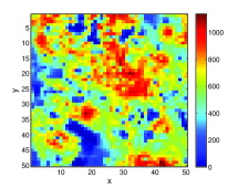
(g) MC, $p=33\%$

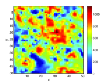
(h) MC, $p=66\%$

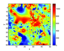
(i) MC, $L_{B}=20$

Figure 8: Visual comparison of magentaMPR, IDW and MC interpolated maps for the Walker lake data shown in Fig. 5(c). Three different patterns of missing data are used: 33% random thinning (left column), 66% random thinning (middle column) and solid block removal (right column). The perimeter of the missing data block is marked by the dashed-line.

The magentaMPR predictions represent conditional means over $M$ equilibrium realizations generated by means of conditional simulation. Hence, even though the magentaMPR predictions are relatively smooth, the prediction variance is appreciable, as shown in Fig. 9(a) for the Walker lake data. In addition, visual supervision of individual magentaMPR-reconstructed realizations in Figs. 9(b)-9(d) demonstrate that the intra-block spatial variability is well reconstructed and that the patterns look “natural”.

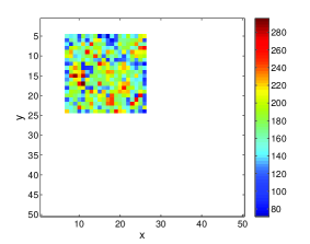
(a) Standard deviation

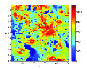
(b) Realization 1

(c) Realization 2

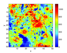
(d) Realization 3

Figure 9: Investigation of magentaMPR conditional simulations of Walker lake data with a missing square block: (a) Standard deviation of block values based on $M=100$ equilibrium realizations. (b)-(d) Three selected realizations (the area of the missing block in the upper left corner is indicated by means of the thin dashed line).

IV.3 Comparison with the Gaussian model

Given the resemblance of the magentaMPR energy function (3) with the quadratic form, one may wonder if the magentaMPR model has any advantages over the simpler Gaussian model. The latter is analytically solvable and has been applied in data reconstruction problems such as the image restoration (Tanaka and J. Inoue,, 2002; Kuwatani et al.,, 2014; Katakami et al.,, 2017). There are two approaches for implementing the latter. In the first, the energy is expressed as a quadratic function of the original field values $z_{i}$, and in the second as a quadratic function of the respective spin angles. Since the first approach strongly penalizes large deviations from the mean, we opted for the second.

In the following, we compare the gap-filling performance of the magentaMPR model, which is defined by the pair interactions $H_{ij}=\cos[q\Delta\phi_{ij}]$ with the GMRF, which is defined by the pair interactions $H_{ij}=-\Delta\phi_{ij}^{2}/2\pi^{2}+1$. In both cases, the energy is given by ${\mathcal{H}}=-\sum_{\langle i,j\rangle}H_{ij}$, while the spin angle contrast takes values $\Delta\phi_{ij}=\phi_{i}-\phi_{j}\in[-2\pi,2\pi]$, and the pair interactions $H_{ij}\in[-1,1]$.

Based on the comparison between the SEM method and maximum likelihood estimation (MLE) that give practically identical results for the one-dimensional magentaMPR model (see Section V.1.2 below), we estimated parameters for both the magentaMPR and the GMRF using SEM. The magentaMPR sample specific energy for temperature inference is given by (4), while the corresponding GMRF sample specific energy is given by

$$e_{s}=\frac{1}{N_{SP}}\sum_{i=1}^{N}\sum_{j\in nn(i)}(\phi_{i}-\phi_{j})^{2}/2\pi^{2}-1.$$

As evidenced in the upper part of Table 6, for synthetic Gaussian data with various WM covariance parameters, there are no significant differences between the gap filling performance of the two models. This is not surprising, since for symmetric Gaussian data the two models behave quite similarly.

However, the differences between the two models can be substantial for data with non-Gaussian distributions. In the lower part of Table 6 we present results for synthetic data that follow the lognormal distribution, i.e., $\log Z\sim N(m=5,\sigma=1)$ and different parametrization of the WM covariance. Hence, the lognormal random field that generates the data has a median $z_{0.50}=\exp(m)\approx 148.41$ and a respective standard deviation of $\sigma_{Z}=\left[\exp(\sigma^{2})-1\right]^{1/2}\exp(\mu+\sigma^{2}/2)\approx 320.75$. The resulting probability distribution thus has a right tail that extends to large positive values.

For all the cases examined, the magentaMPR model validation measures are clearly superior to the GMRF. In addition, the CPU time is practically the same for both models, in spite of the higher computational cost of the cosine compared to the quadratic function. The reason is that the evaluation of the energy function represents a relatively small fraction of the total CPU time. Nevertheless, as mentioned above, the GMRF admits an explicit solution that does not require MC simulations (Tanaka and J. Inoue,, 2002; Kuwatani et al.,, 2014; Katakami et al.,, 2017).

As stated above, in 1D systems the SEM and ML parameter estimation methods yield similar results. Nonetheless, in order to eliminate any potential impact of parameter inference in the 2D system on prediction performance, in Fig. 10 we plot the validation measures for both the magentaMPR and the GMRF models as functions of the temperature. For the Gaussian data (left column) the validation measures and their optimal values are similar for both models (notice the scale of the vertical axes). On the other hand, for the lognormal data (right column) all the magentaMPR validation measures are superior to their GMRF counterparts over the entire temperature range.

Table 6: Comparison of the interpolation validation measures for the magentaMPR method with the magentaMPR $H_{ij}=\cos[q(\phi_{i}-\phi_{j})]$ and GMRF $H_{ij}=-(\phi_{i}-\phi_{j})^{2}/2\pi^{2}+1$ pair interaction functions. $S=100$ samples are generated from the Gaussian $Z\sim N(m=50,\sigma=10)$ and lognormal $\log Z\sim N(m=5,\sigma=1)$ random fields, on a square grid with side length $L=32$. Four covariance models, WM($\kappa,\nu$), with $\kappa=0.2,0.5$ and $\nu=0.25,0.5$ are used. Missing data are generated by (a) $p=33\%$ (b) $p=66\%$ random thinning and (c) random removal of a square data block with side length $L_{B}=20$.

				MAAE			MARE [%]			MAARE [%]			MRASE			MR [%]			$\langle t_{\mathrm{cpu}}\rangle$
Distr.	$\nu$	$\kappa$	$H_{ij}$	(a)	(b)	(c)	(a)	(b)	(c)	(a)	(b)	(c)	(a)	(b)	(c)	(a)	(b)	(c)	(a)	(b)	(c)
Gaussian	0.5	$0.5$	magentaMPR	5.23	5.77	7.34	$-$2.06	$-$2.47	$-$4.16	11.14	12.34	15.98	6.63	7.29	9.23	70.54	62.42	24.47	0.03	0.04	0.03
			Gauss	5.22	5.78	7.32	$-$2.08	$-$2.47	$-$3.99	11.14	12.37	15.93	6.63	7.31	9.20	70.53	62.26	25.17	0.03	0.04	0.03
		$0.2$	magentaMPR	3.48	4.03	7.05	$-$1.08	$-$1.46	$-$5.60	7.41	8.70	16.49	4.36	5.10	9.10	90.66	87.12	45.95	0.03	0.04	0.03
			Gauss	3.49	4.05	7.10	$-$1.09	$-$1.46	$-$5.46	7.43	8.73	16.56	4.37	5.12	9.17	90.59	87.00	45.10	0.03	0.04	0.03
	0.25	$0.5$	magentaMPR	6.83	7.11	7.74	$-$2.95	$-$3.41	$-$8.77	14.67	15.35	17.66	8.64	9.07	9.74	45.59	37.30	11.64	0.03	0.04	0.03
			Gauss	6.83	7.11	7.74	$-$2.96	$-$3.42	$-$9.07	14.67	15.35	17.70	8.64	9.07	9.73	45.68	37.23	12.17	0.03	0.04	0.03
		$0.2$	magentaMPR	5.50	5.81	6.72	$-$1.74	$-$1.90	$-$2.20	11.54	12.19	13.88	6.86	7.32	8.47	65.93	59.84	27.53	0.03	0.04	0.03
			Gauss	5.50	5.82	6.62	$-$1.77	$-$1.92	$-$2.38	11.55	12.21	13.72	6.87	7.33	8.35	65.84	59.72	29.52	0.03	0.04	0.043
lognormal	0.5	$0.5$	magentaMPR	129.27	159.53	385.47	$-$75.82	$-$137.23	$-$477.32	101.91	157.80	482.10	204.73	226.69	430.15	58.55	48.92	9.67	0.03	0.04	0.03
			Gauss	135.63	175.26	464.64	$-$91.84	$-$167.22	$-$571.52	114.82	184.28	574.94	208.11	237.41	509.93	57.49	47.10	7.05	0.03	0.04	0.03
		$0.2$	magentaMPR	94.29	122.05	304.22	$-$45.68	$-$102.72	$-$468.40	66.46	120.65	474.34	152.03	178.21	345.64	83.48	77.53	29.67	0.03	0.04	0.03
			Gauss	98.39	133.20	348.69	$-$58.12	$-$128.42	$-$540.95	76.84	144.03	545.85	153.72	185.62	388.15	83.19	76.31	25.66	0.03	0.04	0.03
	0.25	$0.5$	magentaMPR	174.32	214.51	641.86	$-$111.63	$-$203.28	$-$826.90	142.83	224.25	829.20	311.83	336.86	708.91	25.58	15.30	-2.11	0.03	0.04	0.03
			Gauss	188.23	251.07	833.25	$-$141.66	$-$264.21	$-$1051.75	167.57	280.22	1053.09	325.58	365.79	900.42	22.04	13.07	2.62	0.03	0.04	0.03
		$0.2$	magentaMPR	134.54	166.64	414.54	$-$69.55	$-$131.57	$-$442.22	96.93	151.55	442.22	220.83	244.32	462.01	50.44	39.63	10.08	0.03	0.04	0.03
			Gauss	142.19	188.23	521.53	$-$87.84	$-$168.33	$-$548.43	111.19	184.30	551.04	225.85	259.71	569.52	48.61	37.24	8.41	0.03	0.04	0.03

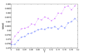
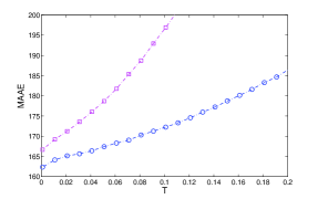
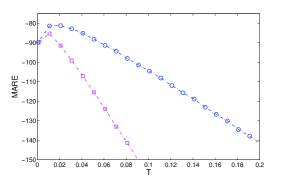
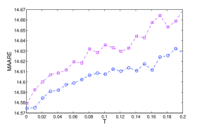
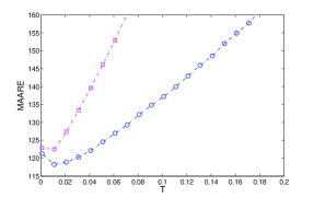
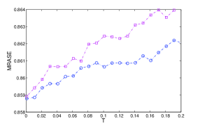
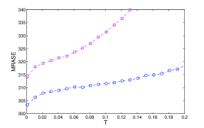
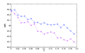
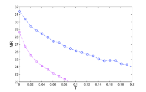
Figure 10: Validation measures versus temperature for the GMRF (magenta squares) and magentaMPR (blue circles) energy functions, using samples from the Gaussian distribution, $Z\sim N(m=5,\sigma=1,\kappa=0.5,\nu=0.25)$ (left column), and the lognormal distribution, i.e., $\log Z\sim N(m=5,\sigma=1)$ (right column) on a square grid of size $L=32$ with $p=33\%$ random thinning.

The advantage of the magentaMPR over the GMRF is due to the fact that the former has higher probability for larger spin angle contrasts, i.e., larger differences between neighboring values of the spin angles. Since skewed data with heavier than normal right tail (e.g., following the lognormal distribution) can lead to spatial configurations with larger contrasts, the magentaMPR model is more suitable than the GMRF.

We conducted a number of numerical experiments to confirm and investigate the above hypothesis. In particular, we generated $S=500$ spatial configurations with $p=33\%$ missing data from the same lognormal random field realization with WM correlations determined by $\kappa=0.5$ and $\nu=0.25$. We sampled the spin angle contrasts $\Delta\phi$ at all the prediction sites in the equilibrium regime of the simulations. We then constructed the spin angle contrast histogram based on the contrast values sampled in the equilibrium regime. The histogram frequencies are obtained by dividing the cumulative frequency of occurrence with the number of the prediction sites, the number of nearest neighbors (four) per site, and the number of MC sweeps in the equilibrium regimes. The resulting histograms approximate the probability density function of the nearest-neighbor spin-angle contrast $\Delta\phi$. We also compare in Fig. 11 the histograms obtained from the GMRF and magentaMPR model predictions with histograms of the true values at the prediction sites. The latter are obtained based on the 500 data sets that are removed from the full realization to generate the missing data configurations.

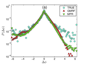
Figure 11: Histograms of (a) spin-angle contrast, $\Delta\phi$, and (b) spin angle, $\phi$, obtained by simulations of the GMRF and magentaMPR energy functions as well as true values, for lognormal data. The inset in (b) shows a magnified view at small $\phi$. The histograms are based on results obtained from 500 missing data configurations that are generated from the same field realization by means of 33% random thinning.

As it is evident in Fig. 11 both the GMRF and magentaMPR histograms overestimate smaller contrasts and underestimate the larger ones. Nevertheless, it is apparent that extremely large contrasts of about $|\Delta\phi|\gtrsim 5$ are better reproduced using the magentaMPR model. Inspection of the spin angle ($\phi$) histograms, shown in Fig. 11, reveals slightly fatter tails in the magentaMPR histogram, which better approximate those of the true values. Note that the histogram of the true values exhibit considerable fluctuations. This is due to the significant variance of the simulated lognormal distribution and the finite probability for very large (extreme) values as discussed above.

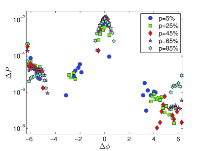
Figure 12: Difference of the spin-angle contrast histograms, $\Delta P=P_{\rm MPR}(\Delta\phi)-P_{\rm GMRF}(\Delta\phi)$, for lognormal data obtained using the magentaMPR and GMRF models for datasets with different degrees of sparsity (percentage of missing points). The histograms are based on results from 500 missing data configurations that are generated from the same field realization.

Differences between the magentaMPR and GMRF spin-angle contrast histograms also appear at other contrasts and persist even when the data sparsity changes. Fig. 12 shows the difference $\Delta P=P_{\rm MPR}(\Delta\phi)-P_{\rm GMRF}(\Delta\phi)$ between the magentaMPR and GMRF histograms for the cases when $P_{\rm MPR}(\Delta\phi)>P_{\rm GMRF}(\Delta\phi)$  and for different thinning degrees $p$. It is evident that the thicker tails in the magentaMPR histogram observed for $p=33\%$ (cf. Fig. 11) persist for all the studied sparsity values. Small contrast values of $|\Delta\phi|\lesssim 0.65$ are also more frequent in the magentaMPR realizations, while the GMRF model has higher frequency at certain intermediate values.

Based on the evidence examined above, we conclude that the magentaMPR model has the advantage over the GMRF with respect to filling gaps in skewed, non-Gaussian spatial data. The magentaMPR’s performance is due to a combination of factors that include the probability distribution of the dataset as well as the properties of the spatial correlation function (the latter has not been investigated).

In future research it is possible to generalize the magentaMPR model by introducing additional parameters to control non-linearity, e.g., by including higher-order interactions (Žukovič and Kalagov,, 2017), and to capture other common features of spatial data, such as geometric anisotropy and non-stationarity.

V Discussion

V.1 Model parameter inference

The reduced temperature is the only parameter of the magentaMPR model that needs to be inferred from the data. In the case of spin models, standard statistical inference procedures, e.g., maximum likelihood estimation, are not easy to apply. The problem is the calculation of the partition function (normalizing factor), which is intractable even for moderately large systems. Consequently, one has to resort to tractable approximations. However, some approximate solutions, such as the maximum pseudolikelihood approach or Markov chain Monte Carlo techniques, can be inaccurate or/and prohibitively slow for large data sets. As described in Section II.3, we use the SEM principle to estimate the temperature, ${\hat{T}}$, used in the magentaMPR conditional simulation.

V.1.1 Performance of the SEM approach

To test the performance of the SEM temperature estimator, we compare ${\hat{T}}$ inferred from various samples with the “optimal” temperature $T_{\textrm{opt}}$. For each sample, $T_{\textrm{opt}}$ is defined by means of

$$T_{\textrm{opt}}=\sum_{i}w_{i}T_{\textrm{opt},i},$$ (12)

where $T_{\textrm{opt},i}$ is the temperature that optimizes the i-th validation measure, ${\rm VM}_{\textrm{opt},i}$, and VM= { AAE, ARE, AARE, RASE, R }. Hence, the lowest values are optimal for AAE, ARE, AARE, and RASE, while the highest value is optimal for $R$. The coefficients $w_{i}$ $(i=1,\ldots,5)$ represent weights defined as follows

$$w_{i}={\Big{|}}({\rm VM}_{\textsc{SEM},i}-{\rm VM}_{\textrm{opt},i})/{\rm VM}_{\textsc{SEM},i}{\Big{|}}{\Big{/}}\sum_{i}{\Big{|}}({\rm VM}_{\textsc{SEM},i}-{\rm VM}_{\textrm{opt},i})/{\rm VM}_{\textsc{SEM},i}{\Big{|}},$$ (13)

where ${\rm VM}_{\textsc{SEM},i}$ is the validation measure at the temperature ${\hat{T}}$ inferred by SEM.

As evidenced in the results for the synthetic WM($\kappa=0.2,\nu=0.5$) data that are presented in Fig. 13, there is considerable variation between the inferred temperatures using SEM and the optimal values $T_{\textrm{opt}}$. Namely, SEM tends to overestimate $T_{\textrm{opt}}$, especially in the case of randomly thinned data.

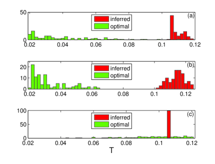
Figure 13: Histograms of temperature values ${\hat{T}}$, inferred from the energy, vs. the optimal values ${T}_{\textrm{opt}}$, giving overall the best validation measures, based on $S=100$ samples of WM($\kappa=0.2,\nu=0.5$) data with $L=256$, generated by (a) $p=33\%$, (b) $p=66\%$ random thinning and (c) random removal of a solid block of data of the side length $L_{B}=20$.

Next, we investigate the impact on prediction performance of using optimal temperatures instead of the SEM estimates by repeating the magentaMPR simulations at temperatures $T_{\textrm{opt}}$ and analyzing the validation measures thus obtained. Table 7 lists the relative validation measures ${\rm VM^{*}}={\rm VM}_{\textrm{opt}}/{\rm VM}_{\textsc{SEM}}$ for the synthetic data with $L=256$. As expected, the overall prediction performance improves by using $T_{\textrm{opt}}$. Nevertheless, considering the large differences between the ${\hat{T}}$ inferred from SEM and $T_{\textrm{opt}}$, the relative differences between the respective validation measures are surprisingly small, typically $\approx 0.1\%$. These results support the robustness of the magentaMPR method against fluctuations of $\hat{T}$ that might result from the presence of noise and outliers, or from limited inference precision due to small sample size or data sparsity.

Table 7: Relative validation measures ${\rm VM^{*}}={\rm VM}_{\textrm{opt}}/{\rm VM}_{\textsc{SEM}}$ obtained as the ratio of the validation measure based on the optimal temperature $T_{\textrm{opt}}$ over the same measure based on the temperature ${\hat{T}}$ estimated by means of specific energy matching. $S=100$ samples are generated from a Gaussian random field with mean equal to 50 on a square grid with side length $L=256$. Two covariance models, WM($\kappa=0.2,\nu=0.5$) and WM($\kappa=0.2,\nu=0.25$) are used. Missing data are generated by (a) $p=33\%$ (b) $p=66\%$ random thinning and (c) random removal of square data block with side length $L_{B}=20$ (same data as in Table 4 for $L=256$). Boldfaced values mark cases for which the validation measure obtained at $T_{\textrm{opt}}$ is inferior to that obtained at ${\hat{T}}$.

	${\rm MAAE^{*}}$			${\rm MARE^{*}}$			${\rm MAARE^{*}}$			${\rm MRASE^{*}}$			MR∗
$\nu$	(a)	(b)	(c)	(a)	(b)	(c)	(a)	(b)	(c)	(a)	(b)	(c)	(a)	(b)	(c)
$0.25$	1.00	1.00	1.00	1.00	1.00	0.94	1.00	1.00	0.99	1.00	1.00	1.00	1.00	1.00	1.02
$0.5$	1.00	1.00	1.00	1.00	1.00	1.02	1.00	1.00	1.00	1.00	1.00	1.00	1.00	1.00	1.01

V.1.2 Comparison of SEM and MLE approaches in 1D

As stated above, the SEM-based procedure seems to overestimate the temperature with respect to the “optimal” value, at least in configurations involving randomly missing data. This effect diminishes in denser data sets. However, the “optimality criterion” (12) is based on an ad hoc linear combination of various validation measures, since the standard MLE procedure cannot be applied to 2D data.

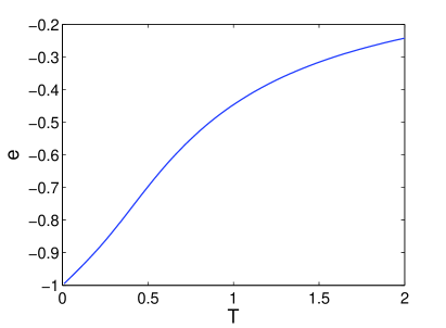
Figure 14: Specific energy of the 1D magentaMPR model as a function of temperature based on (16).

To test the reliability of SEM parameter inference, we compare it below with MLE for the one-dimensional (1D) magentaMPR model. The partition function of the magentaMPR chain with an open boundary condition admits a closed-form expression (Tanemura,, 1994) as

$$Z(\beta)=I_{0}(\beta)^{N-1},$$ (14)

where $\beta=1/T$ is the inverse temperature, $N$ is the chain length, and $I_{0}$ is the modified Bessel function of the first kind, which leads to the following log-likelihood function

$$\log L(\beta,\Phi_{s})=-\beta E_{s}-N_{SP}\log I_{0}(\beta).$$ (15)

In the above, $\Phi_{s}$ represent the sample data, $E_{s}=-\sum_{i=1}^{N}\cos[q(\phi_{i}-\phi_{i+1})]$ is the total sample energy calculated from the nearest-neighbor sample values and $N_{SP}$ is the number of the nearest-neighbor sample pairs.

The MLE estimates $\hat{T}=1/\hat{\beta}$ are obtained by minimizing numerically $-\log L(\beta,\Phi_{s})$, i.e., the negative log-likelihood (NLL). We perform the optimization with the gradient-free Nelder-Mead simplex search algorithm. The termination criteria are that both $\beta$ and the NLL cost function change less than $\epsilon=10^{-6}$ between consecutive steps. The initial guess for the inverse temperature is $\beta^{(0)}=1$. The algorithm was implemented using the Matlab® function fminsearch.

For the SEM method we need the specific (internal) energy. Knowing the partition function, the latter can be obtained in closed form as follows

$$e=-\frac{1}{N-1}\frac{\partial}{\partial\beta}\log Z(\beta)=-I_{1}(\beta)/I_{0}(\beta).$$ (16)

The temperature dependence of the 1D-magentaMPR specific energy is plotted in Fig. 14. The SEM temperature for a given sample is obtained as the value corresponding to the sample’s specific energy $e_{s}=E_{s}/N_{SP}$, i.e., by means of $\hat{T}=e^{-1}(e_{s})$.

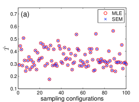
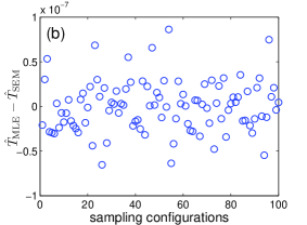
Figure 15: (a) Temperature estimates for the 1D magentaMPR model obtained by means of MLE (red circles) and SEM (blue crosses). (b) Difference of the respective SEM and MLE estimates.

To compare the MLE and SEM temperature estimates, we performed tests on synthetic data mirroring those used for the 2D case. Namely, we first generated a 1D data (time series) of length $N=100$ from the Gaussian distribution $Z\sim N(m=50,\sigma=10)$ with WM covariance parameters $\kappa=0.5,\nu=0.25$. Then we randomly removed $p=33\%$ of the data to generate $S=100$ different sampling configurations. As shown in Fig. 15 both MLE and SEM lead to practically identical estimates. Fig. 15 displays the difference between the respective SEM and MLE estimates, the values are smaller in magnitude than the tolerance $\epsilon=10^{-6}$ used for MLE optimization. These results demonstrate that the SEM estimates are as reliable as the MLE ones, at least in the 1D case.

V.2 Computational efficiency

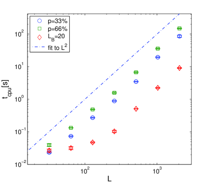
Figure 16: CPU time scaling versus the grid size $L$ based on $S=100$ samples of WM($\kappa=0.2,\nu=0.5$) data. Three plots generated by $p=33\%$ random thinning (circles), $p=66\%$ random thinning (squares), and random removal of a solid block with side length $L_{B}=20$ (diamonds) are shown. The dash-dot line is a guide to the eye for linear dependence.

The computational efficiency of the magentaMPR approach crucially depends on an efficient updating scheme that can bring the system to thermodynamic equilibrium as fast as possible. After equilibrium is established, a predefined number of realizations can be sampled to derive predictive means. The hybrid algorithm that combines restricted Metropolis and over-relaxation dynamics provides such an updating scheme. The resulting relaxation time in terms of MC sweeps is of the order of tens of hybrid sweeps even for the largest grid sizes considered, and it seems to plateau at this level. Additionally, the short-range nature of the interaction between the spin variables enables vectorization by means of the checkerboard algorithm, so that each sweep can be completed in just two steps. Naturally, the physical CPU time per sweep, and thus also the total CPU time $t_{\mathrm{cpu}}$ (including both the relaxation and sampling time), is expected to increase with data size. In Fig. 16 we plot the total CPU time as a function of the data size obtained based on $S=100$ simulations of Gaussian data with WM($\kappa=0.2,\nu=0.5$) and different patterns of missing values. The log-log plots indicate that, at least on grids with side length up to $L=2048$, the CPU time does grow at most linearly with the data size.

VI Conclusions and Further Research

We have introduced a novel Gibbs Markov random field based on the modified planar rotator (magentaMPR) model. Unlike the well-known non-Gaussian Ising model that is suitable for binary-valued data, the magentaMPR model is applicable to continuous data that take values in a closed subset of the real numbers. The magentaMPR is amenable to computationally efficient conditional simulation suitable for the reconstruction of missing data on regular spatial grids. Hence, it is useful for the imputation of missing data in remote sensing datasets (e.g., satellite and airborne lidar data). The computational efficiency derives from the local nature of the spin interactions and the use of a hybrid Monte Carlo simulation algorithm.

Using empirical tests on both randomly missing and contiguous missing block data, we have demonstrated the competitiveness of magentaMPR with respect to several interpolation methods used for gap filling. The magentaMPR model is promising for automated processing of partially sampled data sets due to its simplicity, computational efficiency, and dependence on a single tunable parameter (temperature). The latter can be estimated without user supervision, thus making the magentaMPR model suitable for the automated prediction of missing data.

Another important feature is the potential of the magentaMPR algorithm to process big data in near real-time. This goal requires further gains in efficiency and memory use optimization that can be achieved through parallelization of the algorithm. Such parallelization is feasible due to the short-range (nearest-neighbor) nature of the interactions between the magentaMPR variables (spins). Recent developments in spin model simulations (Weigel,, 2012), as well as our preliminary tests, have demonstrated that much larger data sizes can be handled, and significant speed-ups by factors of up to $1000$ can be achieved by using a highly parallel architecture of graphics processing units (GPUs).

One may wonder whether the advantage of the magentaMPR model that derives from its dependence on a single parameter limits the scope of its applications. The flexibility of the model can be enhanced at some computational cost. One possibility is to allow the model to automatically select the optimal value of $q$ in the interval $[0,1/2]$ by means of a cross-validation procedure —instead of arbitrarily setting it equal to $1/2$. In order to better capture additional spatial features, such as geometric anisotropy or non-stationarity, potentially necessary for huge Earth observation data sets over extended spatial domains, additional coupling parameters can be introduced. Possible extensions in this direction include the generalization of the magentaMPR Hamiltonian by incorporating (i) exchange interaction anisotropy (ii) an external “magnetic” field that can generate spatial trends and (iii) interactions beyond nearest neighbors. Furthermore, the double-checkerboard decomposition that enables processing data in several non-overlapping windows can provide computational benefits for the modeling of nonstationary and/or anisotropic data (Weigel,, 2012).

The magentaMPR model could also be extended to irregularly spaced data by means of kernel functions, in the spirit of stochastic local interaction models (Hristopulos,, 2015). However, in the case of irregularly spaced data some of the computational efficiency that derives from the lattice geometry will be sacrificed. Another appealing direction is the extension of the present approach to three dimensions, where efficient methods for modeling large spatio-temporal data sets are still lacking (Wang et al.,, 2012).

References

- Bechle et al., (2013) M. J. Bechle, D. B. Millet, and J. D. Marshall, Remote sensing of exposure to NO2: satellite versus ground based measurement in a large urban area, Atmos. Environ. 69, 345 (2013).
- Coleman et al., (2011) J. B. Coleman, X. Yao, T. R. Jordan, and M. Madden, Holes in the ocean: Filling voids in bathymetric lidar data. Comput. Geosci. 37, 474 (2011).
- Kadlec and Ames, (2017) J. Kadlec and D. P. Ames, Using crowdsourced and weather station data to fill cloud gaps in MODIS snow cover datasets, Environ. Model. Softw. 95, 258 (2017).
- Lehman et al., (2004) J. Lehman, K. Swinton, S. Bortnick, C. Hamilton, E. Baldridge, B. Eder, and B. Cox, Spatio-temporal characterization of tropospheric ozone across the eastern United States., Atmos. Environ. 38 (26), 4357 (2004).
- Sun et al., (2017) L. Sun, Z. Chen, F. Gao, M. Anderson, L. Song, L. Wang, B. Hu, and Y. Yang, Reconstructing daily clear-sky land surface temperature for cloudy regions from MODIS data, Comput. Geosci. 105, 10 (2017).
- Yoo et al., (2010) C, Yoo, J. Yoon, and E. Ha, Sampling error of areal average rainfall due to radar partial coverage, Stoch. Environ. Res. Risk Assess. 24, 1097 (2010).
- Sickles and Shadwick, (2007) J. E. Sickles and D. S. Shadwick, Effects of missing seasonal data on estimates of period means of dry and wet deposition, Atmos. Environ. 41 (23), 4931 (2007).
- Wackernagel, (2003) H. Wackernagel, Multivariate Geostatistics (Springer, New York, 2003).
- Sun et al., (2009) Y. Sun, S. Kang, F. Li, and L. Zhang, Comparison of interpolation methods for depth to groundwater and its temporal and spatial variations in the Minqin oasis of northwest China, Environ. Model. Softw. 24, 1163 (2009).
- Diggle and Ribeiro, (2007) P. J. Diggle, P. J. Ribeiro, Jr., Model-based Geostatistics, (Springer series in statistics, New York, 2007).
- Pebesma and Wesseling, (1998) E. J. Pebesma and C. G. Wesseling, Gstat: a program for geostatistical modelling, prediction and simulation, Comput. Geosci. 24 (1), 17 (1998).
- Cressie and Johannesson, (2008) N. Cressie and G. Johannesson, Fixed rank kriging for very large spatial data sets, J. R. Stat. Soc.: Ser. B (Stat. Methodol.) 70 (1), 209 (2008).
- Furrer et al., (2006) R Furrer, M. G. Genton, and D. Nychka, Covariance tapering for interpolation of large spatial datasets, J. Comput. Graph. Stat. 15 (3), 502 (2006).
- Ingram et al., (2008) B. Ingram, D. Cornford, and D. Evans, Fast algorithms for automatic mapping with space-limited covariance functions, Stoch. Environ. Res. Risk Assess. 22, 661 (2008).
- Kaufman et al., (2008) C. G. Kaufman, M. J. Schervish, and D. W. Nychka, Covariance tapering for likelihood-based estimation in large spatial data sets, J. Am. Stat. Assoc. 103 (484), 1545 (2008).
- Marcotte and Allard, (2017) D. Marcotte and D. Allard, Half-tapering strategy for conditional simulation with large datasets, Stoch Environ Res Risk Assess 32, 279 (2018).
- Zhong et al., (2016) X. Zhong, A. Kealy, and M. Duckham, Stream Kriging: Incremental and recursive ordinary Kriging over spatiotemporal data streams, Comput. Geosci. 90, 134 (2016).
- Cheng, (2013) T. Cheng, Accelerating universal Kriging interpolation algorithm using CUDA-enabled GPU, Comput. Geosci. 54, 178 (2013).
- Gutiérrez de Ravé et al., (2014) E. Gutiérrez de Ravé, F. J. Jiménez-Hornero, A. B. Ariza-Villaverde, and J. M. Gómez-López, Using general-purpose computing on graphics processing units (GPGPU) to accelerate the ordinary kriging algorithm, Comput. Geosci. 64, 1 (2014).
- Hu and Shu, (2015) H. Hu and H. Shu, An improved coarse-grained parallel algorithm for computational acceleration of ordinary Kriging interpolation, Comput. Geosci. 78, 44 (2015).
- Pesquer et al., (2011) L. Pesquer, A. Cortés, and X. Pons, Parallel ordinary kriging interpolation incorporating automatic variogram fitting, Comput. Geosci. 37, 464 (2011).
- Hristopulos, (2003) D. T. Hristopulos, Spartan Gibbs random field models for geostatistical applications, SIAM J. Scient. Comput. 24 (6), 2125 (2003).
- Hristopulos and Elogne, (2007) D. T. Hristopulos and S. N. Elogne, Analytic properties and covariance functions for a new class of generalized Gibbs random fields, IEEE Trans. Inform. Theor. 53 (12), 4467 (2007).
- (24) M. Žukovič and D. T. Hristopulos, Classification of missing values in spatial data using spin models. Phys. Rev. E 80, 011116-1-23 (2009).
- (25) M. Žukovič and D. T. Hristopulos, Multilevel discretized random field models with “spin” correlations for the simulation of environmental spatial data. J. Stat. Mech.: Theory and Experiment, P02023-1-20 (2009).
- (26) M. Žukovič and D. T. Hristopulos, Reconstruction of missing data in remote sensing images using conditional stochastic optimization with global geometric constraints, Stoch. Environ. Res. Risk Assess. 27 (4), 785 (2013).
- (27) M. Žukovič and D. T. Hristopulos, A Directional Gradient-Curvature method for gap filling of gridded environmental spatial data with potentially anisotropic correlations, Atmos. Environ. 77, 901 (2013).
- Rue and Held, (2005) H. Rue and L. Held, Gaussian Markov Random Fields: Theory and Applications, (CRC press, Boca Raton, FL, 2005).
- Gelfand et al., (2010) A. E. Gelfand, P. Diggle, P. Guttorp, and M. Fuentes (eds.), Handbook of Spatial Statistics, (CRC Press, Boca Raton, FL, 2010).
- Besag, (1974) J. Besag, Spatial interaction and the statistical analysis of lattice systems, J. R. Stat. Soc. Ser. B 36 (2), 192 (1974).
- Nishimori and Wong, (1999) H. Nishimori and K. Y. M. Wong, Statistical mechanics of image restoration and error-correcting codes, Phys. Rev. E 60, 132 (1999).
- Wong and Nishimori, (2000) K. Y. M. Wong and H. Nishimori, Error-correcting codes and image restoration with multiple stages of dynamics, Phys. Rev. E 62, 179 (2000).
- Inoue, (2001) J. Inoue, Application of the quantum spin glass theory to image restoration, Phys. Rev. E 63, 046114-1-10 (2001).
- Inoue, (2001) J. Inoue, and D. M. Carlucci, Image restoration using the Q-Ising spin glass, Phys. Rev. E 64, 036121-1-18 (2001).
- Tadaki and Inoue, (2001) T. Tadaki and J. Inoue, Multistate image restoration by transmission of bit-decomposed data, Phys. Rev. E 65, 016101-1-13 (2001).
- Saika and Nishimori, (2002) Y. Saika and H. Nishimori, Statistical mechanics of image restoration by the plane rotator model, J. Phys. Soc. Jpn. 71, 1052 (2002).
- Žukovič and Hristopulos, (2015) M. Žukovič and D. T. Hristopulos, Short-range correlations in modified planar rotator model, J. Phys.: Conf. Ser. 633, 012105-1-8 (2015).
- Chaikin and Lubensky, (2000) P. M. Chaikin and T. C. Lubensky, Principles of Condensed Matter Physics, (Cambridge University press, 2000).
- Kosterlitz and Thouless, (1973) J. M. Kosterlitz and D. J. Thouless, Ordering, metastability and phase transitions in two-dimensional systems, J. Phys. C 6, 1181 (1973).
- Creutz, (1987) M. Creutz, Overrelaxation and Monte Carlo simulation, Phys. Rev. D 36, 515 (1987).
- Metropolis et al., (1953) N. Metropolis, A. W. Rosenbluth, M. N. Rosenbluth, A. H. Teller, and E. Teller, Equation of State Calculations by Fast Computing Machines, J. Chem. Phys. 21, 1087 (1953).
- Gupta et al., (1988) R. Gupta, J. DeLapp, G. G. Batrouni, G. C. Fox, C. F. Baillie, and J. Apostolakis, Phase transition in the 2D model, Phys. Rev. Lett. 61 (17), 1996 (1988).
- Savitzky and Golay, (1964) A. Savitzky and M. J. E. Golay, Smoothing and differentiation of data by simplified least squares procedures, Anal. Chem. 36, 1627 (1964).
- Sandwell, (1987) D. T. Sandwell, Biharmonic spline interpolation of GEOS-3 and SEASAT altimeter data, Geophys. Res. Lett. 14, 139 (1987).
- Shepard, (1968) D. Shepard, A two-dimensional interpolation function for irregularly-spaced data, Proceedings of the 1968 ACM National Conference, 517 (1968).
- Howat, (2007) I. M. Howat, Filling NaNs in array using inverse-distance weighting. (http://www.mathworks.com/matlabcentral/fileexchange/15590-fillnans), MATLAB Central File Exchange. Retrieved June 15, 2009.
- Sidler, (2003) R. Sidler, Kriging and conditional geostatistical simulation based on scale-invariant covariance models, Diploma thesis, ETH Zurich, Zurich, Switzerland (2003).
- Pebesma, (2004) E. J. Pebesma, Multivariable geostatistics in S: the gstat package. Comput. Geosci. 30, 683 (2003).
- Pebesma et al., (2016) B. Gräler, E. Pebesma and G. Heuvelink, Spatio-Temporal Interpolation using gstat. The R Journal 8, 204 (2016).
- Li and Heap, (2014) J. Li and A. D. Heap, Spatial interpolation methods applied in the environmental sciences: A review, Environ. Model. Softw. 53, 173 (2014).
- Drummond and Horgan, (1987) I. T. Drummond and R. R. Horgan, The effective permeability of a random medium, J. Phys. A 20, 4661 (1987).
- Minasny and McBratney, (2005) B. Minasny and A. B. McBratney, The Matérn function as a general model for soil variograms, Geoderma 128, 192 (2005).
- Pardo-Igúzquiza and Chica-Olmo, (2008) E. Pardo-Igúzquiza and M. Chica-Olmo, Geostatistics with the Matern semivariogram model: A library of computer programs for inference, kriging and simulation, Comput. Geosci. 34 (9), 1073 (2008).
- Pardo-Igúzquiza et al., (2009) E. Pardo-Igúzquiza, K. V. Mardia, and M. Chica-Olmo, MLMATERN: A computer program for maximum likelihood inference with the spatial Matérn covariance model, Comput. Geosci. 35 (6), 1139 (2009).
- Tao et al., (2006) W.-K. Tao, et al., Retrieval of latent heating from TRMM measurements, Bull. Am. Meteor. Soc. 87 (11), 1555 (2006).
- TRMM, (2011) Tropical Rainfall Measuring Mission (TRMM) (2011), TRMM Microwave Imager Precipitation Profile L3 1 month 0.5 degree x 0.5 degree V7, Greenbelt, MD, Goddard Earth Sciences Data and Information Services Center (GES DISC), Accessed [Sept. 30, 2008] https://disc.gsfc.nasa.gov/datasets/TRMM_3A12_7/summary
- Isaak and Srivastava, (1989) E. Isaak and R. Srivastava, An Introduction to Applied Geostatistics, (Oxford University Press, New York, 1989).
- Cressie, (1985) N. Cressie, Fitting variogram models by weighted least squares, Math. Geol. 17, 563 (1985).
- Žukovič and Kalagov, (2017) M. Žukovič and G. Kalagov, model with higher-order exchange, Phys. Rev. E 96, 022158-1-8 (2017).
- Tanaka and J. Inoue, (2002) K. Tanaka and J. Inoue, Maximum Likelihood Hyperparameter Estimation for Solvable Markov Random Field Model in Image Restoration. IEICE Transactions on Information and Systems 85, 546 (2002).
- Kuwatani et al., (2014) T. Kuwatani, K. Nagata, M. Okada, and M. Toriumi, Markov random field modeling for linear seismic tomography, Phys. Rev. E 90, 042137 (2014).
- Katakami et al., (2017) S. Katakami, H. Sakamoto, S. Murata, and M. Okada, Gaussian Markov random field model without boundary conditions, J. Phys. Soc. Jpn. 86, 064801 (2017).
- Tanemura, (1994) Tanemura, M. (1994): Likelihood estimation of directional interaction. in H. Bozdogan (ed.) Proceedings of the First US/Japan Conference on Frontiers of Statistical Modeling: An Informational Approach, Kluwer, Amsterdam, pp.293-313.
- Weigel, (2012) M. Weigel, Performance potential for simulating spin models on GPU, J. Comput. Phys. 231, 3064 (2012).
- Hristopulos, (2015) D. T. Hristopulos, Stochastic Local Interaction (SLI) model: Bridging machine learning and geostatistics, Comput. Geosci. 85, 26 (2015).
- Wang et al., (2012) G. Wang, D. Garcia, Y. Liu, R. de Jeu, and A. J. Dolman, A three-dimensional gap filling method for large geophysical datasets: Application to global satellite soil moisture observations, Environ. Model. Softw. 30, 139 (2012).