Correlations of cascaded photons: An analytical study in the two-photon Mollow regime

Abstract

Mollow physics in the two-photon regime shows interesting features such as path-controlled time-reordering of photon pairs without the need to delay them. Here, we calculate analytically the two-photon correlations $g^{(2)}(\tau)$, essential to discuss and study such phenomena in the resonant-driven dressed-state regime. It is shown that there exists upper and lower bounds of the $g^{(2)}(\tau)-$ function for certain spectrally-selected photon pairs. Recent reported experiments agree with the presented theory and thereby it is shown that the resonant-driven four-level system is an interesting source for steerable quantum light in quantum cascade setups. We furthermore discuss the unlikeliness to observe antibunching for the delay time $\tau=0$ in the exciton-biexciton correlation functions in such experiments, since antibunching stems from a coherent and in-phase superposition of different photon emission events. Due to the occuring laser photon scattering, this coherent superposition state is easily disturbed and leads to correlation functions of $g^{(2)}(0)=1$.

1 Introduction

Two-photon states are of particular interest to study non-linear phenomena in quantum optics and lie at the heart of the pursuit to exploit nonlocal properties in quantum mechanics itself [1, 2, 3, 4]. Two-photon states generated in an atomic cascade allowed the first experiments to test Bell’s inequality [5, 6, 7, 8] and have paved the way to significant-loophole free tests in other material platforms recently [9, 10]. Nowadays semiconductor based biexciton-cascade processes generate on demand polarized-entangled photon pairs to a very high degree of purity due to recent progresses in nanotechnology fabrication [11, 12, 13, 14]. They also gave rise to test the indistinguishability of photons created in the spontaneous parametric downconversion via Hong-Ou-Mandel type of experiments [15, 16, 1], and semiconductor growth techniques allow now high extraction efficiencies and close to perfect visibilities [17, 18, 19, 20]. Furthermore, two-photon signatures reveal the true quantum character of cavity quantum electrodynamics via anharmonic, second-rung features that scale non-linearly with the photon number. Experimentally, higher-order rungs have been extracted in superconducting circuit platforms [21, 22], atom cavity-QED systems [23, 24] and also in semiconductor nano-emitters clear signatures have been observed [25, 26]. Thus, two-photon sources have a wide application domain and allow to test a broad range of quantum behavior. It is therefore highly feasible to understand two-photon generation processes based on incoherent and coherent driving on an analytical and fundamental level.

Recently, a proposal has drawn interest, which allows one to coherently generate photon bundles in leap-frog processes [27, 28, 29]. The idea behind is to drive the emitter in resonance with the N-photon transition but off-resonant with a single photon coherence [30, 31]. This way, single-photon processes are suppressed which tend to degrade two- or N-photon coherences. Furthermore, the polarization degree of freedom can be used to probe only emission processes without scattered photons from the driving laser field. This idea has been experimentally realized recently with a semiconductor quantum dot [32, 33, 34] . Here, the biexciton is coherently driven in a two-photon process and via only one of the two possible polarization transitions. In the strong driving regime, dressed state become visible and allow for frequency-selected photon-photon correlation measurements [34]. This way, path-controlled time-reordering of photon pairs can be steered. As a measure whether there is and there is no time-order, we use the correlation function and investigate whether the function is symmetric under sign exchange $g^{(2)}(\tau)=g^{(2)}(-\tau)$ or not. If the correlation function is symmetric, the time-order of the emission sequence is erased. Such a vanishing time-reordering is only possible, when the emitter is driven into a superposition state with long coherence times.

Here, we give the theoretical background for the experiment [34] and calculate the correlation functions analytically. We discuss symmetries and also limits for given measurement detection sequences and show, when and under which circumstances perfect time-reordering can be reached, or when anti-correlation is inevitable and bunching will always be the case. We also reveal, which values of the correlation functions values are inaccessible for certain measurement sequences and provide therefore a toolbox to interpret these kind of multi-photon processes with the correlation function data at hand.

The analysis below shows that the physics behind this experiment can still be described with two-level physics, but with a two-photon substructure [3, 35, 36, 37, 38]. The article is organized as follows: After this introduction, cf. 1, we continue in Sec. 2 with presenting the model and discuss the Hamiltonian of the system. The chosen excitation frequency allows to adiabatically eliminate the the exciton levels of the four-level system up to moderate driving strengths. Without the excitonic degrees of freedom, the effective model is isomorph to a two-level system, which can be solved in various ways. We solve it via a Laplace transformation in contrast to most diagonalization approaches common in literature, e.g. [2]. These solutions are interpreted with respect to their two-photon substructure and used to calculate the photon-photon correlation function in the bare state basis in Sec. 3. The results will be a very asymmetric correlation function around $\tau=0$ with antibunching to one side and bunching to the other side. However, in the dressed state basis, derived in Sec. 4, certain contributions show a symmetric behavior. Sec. 5 is dedicated to the calculation of the correlation in the dressed-state basis. Those are the main result of the paper and explain the experimental data of Ref. [34] in case of resonant two-photon excitation. To complete the discussion, intensity dependent experimental data are qualitatively compared to the theory in Sec. 6. The symmetrization of the correlation is clearly seen, now supported additionally via the analytical calculations, before we conclude in Sec. 7.

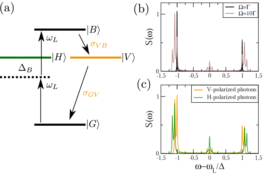
Figure 1: (a) The energy schema of the setup. The biexciton state is driven via a continuous two-photon, $H-$polarized excitation, while the exciton transitions are far detuned. (b) The power spectrum $S(\omega)$ of the full emission, including $H-$ and $V-$polarized photons for two excitation strengths. In the strong excitation limit (grey), triplets appear. (c) Differentiating the spectrum in the strong excitation limit between $H-$ (green,shaded) and $V-$ emission (orange, solid) events. Due to the ignored fine structure splitting $\Delta_{\text{FSS}}=0$ two peaks overlap.

2 Model

The quantum dot is modelled as a four-level system consisting of a ground state $|G\rangle$, two excitonic states $|H\rangle,|V\rangle$ and a biexcitonic state $|B\rangle$. The ground state energy $\omega_{G}=0$ is set to zero, cf. Fig. 1. The two excitonic states may differ in their energies $\omega_{H}-\omega_{V}=\Delta_{\text{FSS}}$ due to the fine structure splitting. This splitting is of great importance in experiments probing photon polarization entanglement generated in a biexciton cascade. Here, we focus on a driven experiment, where photon correlations in the Mollow regime are studied and the fine structure splitting is of minor importance. So, we set it, out of convenience, to zero for the following discussion: $\Delta_{\text{FSS}}=0$, i.e. $\omega_{H}=\omega_{V}=\omega_{X}$. In contrast, the biexciton shift is of particular interest, as only due to this shift it is possible to drive the biexciton population without driving necessarily at the same time the excitonic transitions. The biexciton shift ($\Delta_{B}$) can be attractive or repulsive and is defined as the difference between the sum of the exciton energies and the bare biexciton resonance, rendering the biexciton energy $\omega_{B}=\omega_{H}+\omega_{V}+2\Delta_{B}=2(\omega_{X}+\Delta_{B})$. Here, the external laser field drives only the horizontal polarization with frequency $\omega_{L}$ and amplitude $\Omega_{H}$, the full Hamiltonian reads therefore $(\hbar=1)$ and $\sigma_{ij}:=\left|i\right\rangle\left\langle j\right|$:

$$H= \omega_{X}\left(\sigma_{HH}+\sigma_{VV}\right)+2\left(\omega_{X}+\Delta_{B}\right)\sigma_{BB}+\Omega_{H}\cos(\omega_{L}t)(\sigma_{GH}+\sigma_{HG}+\sigma_{BH}+\sigma_{HB}).$$ (1)

To allow for an adiabatic elimination of the excitonic states in case of biexciton shift in the regime $\Delta_{B}\gg\Omega_{H}$, the laser frequency is chosen to be in a two-photon resonance with the biexciton frequency, namely we set $\omega_{L}=\omega_{H}/2+\omega_{V}/2+\Delta_{B}$. This leads to the following Hamiltonian, assuming $\omega_{H}=\omega_{V}$, and after the rotating-wave approximation and transforming into the rotating frame of the laser frequency:

$$H_{R}= \Delta\left(\sigma_{HH}+\sigma_{VV}\right)+\Omega_{L}(\sigma_{GH}+\sigma_{HG}+\sigma_{BH}+\sigma_{HB}),$$ (2)

with $\Delta=-\Delta_{B}$ and $\Omega_{L}=\Omega_{H}/2$, cf. Fig. 1(a). We assume a radiative decay of the electronic system via photon emission into a Markovian continuum to yield the following master equation:

$$\dot{\rho}= -i\left[H_{R},\rho\right]+\Gamma_{X}\left(\mathcal{D}[\sigma_{GH}]+\mathcal{D}[\sigma_{GV}]+\mathcal{D}[\sigma_{BH}]+\mathcal{D}[\sigma_{BV}]\right)\rho,$$ (3)

after assuming the biexciton decay to be double as fast as the exciton decay and using the standard Lindblad form $\mathcal{D}[J]\rho=2J\rho J^{\dagger}-\{J^{\dagger}J,\rho\}$. Pure dephasing contributions are neglected on this timescale [39] and are set in the master equation, out of convenience, to zero. The following analytical calculations can be done with a finite pure dephasing,rendering them however more lengthy. Since we focus here on the intensity dependent photon-photon correlation in the low temperature limit $T\approx 4K$, where the dissipation in the system is mainly governed by the radiative decay, the pure dephasing is assumed to be of minor importance for the studied correlation function, which is supported also by the intensity-dependent experimental data, in Sec. 6.

In Fig. 1(b) and (c), the power spectrum of the system is plotted: $S(\omega)=\lim\limits_{t\to\infty}\int_{0}^{\infty}\boldsymbol{\big{\langle}}c^{\dagger}(t)c(t+\tau)\boldsymbol{\big{\rangle}}e^{-i\omega\tau}$ with $c(t)=\sigma_{iB}(t)+\sigma_{Gi}(t)$ for $i=H,V$. For weak excitation, only two emission peaks from the bare exciton and bare biexciton photons are visible, cf. Fig. 1(b, black line), since the Mollow splitting is not large enough in comparison to the radiative linewidth. If the driving strength increases, triplets appear around the bare resonances (gray line) and around the laser frequency. To distinguish the contributions, a polarization filter can be applied. The $H-$polarized photons show a very different dependence on the driving strength than the $V-$polarized photons. In contrast to the latter, both peaks of the $H-$polarized photons shift with the driving strength (green, shaded). However, only one peak of the $V-$polarized photons shift (orange solid), and one peak stays independently on the driving strength on the bare resonance.

In the following, the time dynamics of the density matrix is analytically solved. Using the master equation, the following set of differential equations of motion can be derived with $\rho_{ij}=\langle i|\rho|j\rangle$:

$$\dot{\rho}_{GG}= 2\Gamma_{X}(\rho_{HH}+\rho_{VV})-i\Omega_{L}\left(\rho_{HG}-\rho_{GH}\right),$$ (4)

$$\dot{\rho}_{HG}= -\left(\Gamma_{X}+i\Delta\right)\rho_{HG}-i\Omega_{L}\left(\rho_{BG}+\rho_{GG}-\rho_{HH}\right),$$ (5)

$$\dot{\rho}_{HH}= -2\Gamma_{X}\left(\rho_{HH}-\rho_{BB}\right)-i\Omega_{L}\left(\rho_{GH}-\rho_{HG}+\rho_{BH}-\rho_{HB}\right),$$ (6)

$$\dot{\rho}_{BG}= -2\Gamma_{X}\rho_{BG}-i\Omega_{L}\left(\rho_{HG}-\rho_{BH}\right),$$ (7)

$$\dot{\rho}_{BH}= -\left(3\Gamma_{X}-i\Delta\right)\rho_{BH}-i\Omega_{L}\left(\rho_{HH}-\rho_{BB}-\rho_{BG}\right),$$ (8)

$$\dot{\rho}_{BB}= -4\Gamma_{X}\rho_{BB}-i\Omega_{L}\left(\rho_{HB}-\rho_{BH}\right),$$ (9)

$$\dot{\rho}_{VV}= -2\Gamma_{X}\left(\rho_{VV}-\rho_{BB}\right).$$ (10)

Note, the $V$-exciton level is not driven by the external driving field, thus $\rho_{VG}$ and $\rho_{VB}$ and its complex conjugates are no dynamical quantities. Now, we choose a particular quantum dot, where the biexciton shift is much larger than the radiative decay constants, which is typically the case $\Delta\gg\Gamma_{X}$. Furthermore, we choose also a driving strength much weaker than the biexciton binding energy, therefore $\Delta\gg\Omega_{L}$. Therefore, we can eliminate the transition to the $H$ exciton, as the time scale is dominated by the detuning:

$$\rho_{HG}= \frac{i\Omega_{L}}{\Gamma_{X}+i\Delta}\left[\rho_{HH}-\rho_{BG}-\rho_{GG}\right]\approx\frac{\Omega_{L}}{\Delta}\left[\rho_{HH}-\rho_{BG}-\rho_{GG}\right]$$ (11)

$$\rho_{BH}= \frac{i\Omega_{L}}{3\Gamma_{X}-i\Delta}\left[\rho_{BB}+\rho_{BG}-\rho_{HH}\right]\approx-\frac{\Omega_{L}}{\Delta}\left[\rho_{BB}+\rho_{BG}-\rho_{HH}\right],$$ (12)

as we can safely assume $\Delta\gg 3\Gamma_{X}$, as the biexciton energy is in the regime of meV, and the radiative decay constant typically in the domain of $\mu$eV. If we apply these adiabatical solutions into the corresponding equations, and again, ignore the dispersive shifts $\Omega_{L}^{2}/\Delta\ll\Gamma_{X}$, which limits the validity of the following equations to medium driving strength, we yield:

$$\dot{\rho}_{BB}= -4\Gamma_{X}\rho_{BB}+2\text{Im}\left[\frac{\Omega_{L}^{2}}{\Delta}\rho_{BG}\right],$$ (13)

$$\dot{\rho}_{GG}= 2\Gamma_{X}\left(\rho_{HH}+\rho_{VV}\right)-2\text{Im}\left[\frac{\Omega_{L}^{2}}{\Delta}\rho_{BG}\right],$$ (14)

$$\dot{\rho}_{BG}= -2\Gamma_{X}\rho_{BG}-i\frac{\Omega_{L}^{2}}{\Delta}\left(\rho_{BB}-\rho_{GG}\right).$$ (15)

Note, the excitonic densities are no longer a dynamical quantity, they just follow the dissipative dynamics of the biexciton state. So, we can use $\rho_{HH}+\rho_{VV}=\Sigma_{0}-\rho_{BB}-\rho_{GG}$ with typically $\Sigma(t=0)=\Sigma_{0}=1$ and define $\Omega:=2\frac{\Omega_{L}^{2}}{\Delta}$ as the effective two-photon Rabi frequency and $\Gamma:=2\Gamma_{X}$. We have denoted the sum of the initial occupations $\Sigma_{0}$ to include later consistently the solution for different initial conditions in terms of the quantum regression theorem. The solution is easier to calculate for the inversion, i.e. the population difference between biexciton and ground state $D(t):=\rho_{BB}(t)-\rho_{GG}(t)$, and the linear independent imaginary part of the polarization between both states $B(t):=\rho_{BG}(t)-\rho_{GB}(t)$. We yield a closed set of equations of motion:

$$\dot{D}(t)= -\Gamma\left[D(t)+\Sigma_{0}\right]-i\Omega B(t)$$ (16)

$$\dot{B}(t)= -\Gamma B(t)-i\Omega D(t).$$ (17)

Suprisingly, this set of equations is identical with a continuously driven two-level system, see A. We conclude, that the two-photon driven biexciton system is in the adiabatic limit isomorph to the two-level dynamics. However, the underlying structure of the four levels is still present due to the conservation of angular momentum, as the biexciton cannot be driven directly from the ground state but only via an intermediate excitonic state, i.e. $\sigma_{GB}$ corresponds not to a electronic dipole operator. We apply the Laplace transform and rederive the solution of the well-known Mollow problem, see B. In the time domain, the inversion dynamics are given:

$$D(t)= \left(D_{0}+\Sigma_{0}\Gamma\Gamma_{n}\right)e^{-\Gamma t}\cos(\Omega t)-\left(iB_{0}+\Sigma_{0}\Gamma\Omega_{n}\right)e^{-\Gamma t}\sin(\Omega t)-\Sigma_{0}\Gamma\Gamma_{n},$$ (18)

with $\Gamma_{n}=\Gamma/(\Gamma^{2}+\Omega^{2})$ and $\Omega_{n}=\Omega/(\Gamma^{2}+\Omega^{2})$. This equation fulfills the initial condition $D(t=0)=D_{0}$. The general equation of the polarisation dynamics reads:

$$B(t)= \left(B_{0}-i\Sigma_{0}\Gamma\Omega_{n}\right)e^{-\Gamma t}\cos(\Omega t)-i\left(\Sigma_{0}\Gamma\Gamma_{n}+D_{0}\right)e^{-\Gamma t}\sin(\Omega t)+i\Sigma_{0}\Gamma\Omega_{n},$$ (19)

with $B(t=0)=B_{0}$. Given these explicit solutions of the dynamics, all quantities can be derived via integration. For example, the biexciton dynamics reads:

$$\rho_{BB}(t)= \rho_{BB}(0)e^{-2\Gamma t}-iB_{0}\frac{\Omega}{2}e^{-\Gamma t}\left[\Gamma_{n}\cos(\Omega t)+\Omega_{n}\sin(\Omega t)-\Gamma_{n}e^{-\Gamma t}\right]$$ (20)

$$-D_{0}\frac{\Omega}{2}e^{-\Gamma t}\left[\Gamma_{n}\sin(\Omega t)-\Omega_{n}\cos(\Omega t)+\Omega_{n}e^{-\Gamma t}\right]$$ (21)

$$+\Sigma_{0}\frac{\Omega}{2}e^{-\Gamma t}\left[\Omega_{n}\sinh(\Gamma t)-\Gamma_{n}\sin(\Omega t)\right].$$ (22)

The detailed calculation is given in C. So, with the biexciton dynamics at hand, we can derive the ground state dynamics easily due to the definion of $D(t)$:

$$\rho_{GG}(t)= \rho_{BB}(t)-D_{0}e^{-\Gamma t}\cos(\Omega t)+iB_{0}e^{-\Gamma t}\sin(\Omega t)$$ (23)

$$+\Sigma_{0}\Gamma\left[\Gamma_{n}+e^{-\Gamma t}\ \left(\Omega_{n}\sin(\Omega t)-\Gamma_{n}\cos(\Omega t)\right)\right].$$ (24)

For the measurements in the following, the $V-$exciton population is also of importance. If the initial values of both excitonic states are equal, their dynamics agree in the adiabatic limit, as the differential equations in spite of the driving are effectively the same, so one can use $\rho_{HH}(t)=\rho_{VV}(t)$ in case of $\rho_{HH}(0)=\rho_{VV}(0)$. Then, one can conveniently use

$$\rho_{VV}(\tau)=\frac{1}{2}\left(\Sigma_{0}-\rho_{GG}(\tau)-\rho_{BB}(\tau)\right)=\frac{1}{2}\left(\Sigma_{0}+D(\tau)-2\rho_{BB}(\tau)\right),$$ (25)

again typically $\Sigma=1$ but not if the conditional probability in two-time-correlations is calculated. However, if their initial values do not agree, one has to calculate the dynamics explicitly via

$$\rho_{VV}(t)= \rho_{VV}(0)e^{-\Gamma t}+\Gamma e^{-\Gamma t}\int_{0}^{t}dt^{\prime}e^{\Gamma t^{\prime}}\ \rho_{BB}(t^{\prime}).$$ (26)

Finally, the polarisation reads:

$$\rho_{BG}(t)= \frac{1}{2}B(t)+\frac{1}{2}e^{-\Gamma t}(\rho_{BG}(0)+\rho_{GB}(0))$$ (27)

In the following, the exciton-biexciton photon correlations are calculated explicitly to unravel the dependence on the two-photon driving strength $\Omega=2\Omega_{L}^{2}/\Delta$ in comparison to the radiative decay constant $\Gamma=2\Gamma_{X}$.

3 Biexciton-Exciton Photon-Photon Correlation

The measurement setup discriminates between the biexciton and exciton photon through the different frequencies but with the same polarization, here $V$, the undriven transitions. The generation of photons is in the far field proportional to the corresponding transition operator $c^{\dagger}_{ij}(t)=\sigma_{ij}(t)$ [2]. The corresponding intensity-intensity correlation reads:

$$g^{(2)}_{ijkl}(\tau)= \lim\limits_{t\to\infty}\frac{\boldsymbol{\big{\langle}}c^{\dagger}_{ij}(t)c^{\dagger}_{kl}(t+\tau)c^{\phantom{\dagger}}_{lk}(t+\tau)c^{\phantom{\dagger}}_{ji}(t)\boldsymbol{\big{\rangle}}}{\boldsymbol{\big{\langle}}c^{\dagger}_{ij}(t)c^{\phantom{\dagger}}_{ji}(t)\boldsymbol{\big{\rangle}}\boldsymbol{\big{\langle}}c^{\dagger}_{kl}(t)c^{\phantom{\dagger}}_{lk}(t)\boldsymbol{\big{\rangle}}}.$$ (28)

In the density matrix picture, and with the corresponding transition operators, the correlations function is given with

$$\lim\limits_{t\to\infty}\boldsymbol{\big{\langle}}c^{\dagger}_{ij}(t)c^{\dagger}_{kl}(t+\tau)c^{\phantom{\dagger}}_{lk}(t+\tau)c^{\phantom{\dagger}}_{ji}(t)\boldsymbol{\big{\rangle}}\equiv\lim\limits_{t\to\infty}\text{Tr}\left[\rho(0)\sigma_{ij}(t)\sigma_{kl}(t+\tau)\sigma_{lk}(t+\tau)\sigma_{ji}(t)\right]$$

$$=\lim\limits_{t\to\infty}\text{Tr}\left[\left|j\right\rangle\left\langle i\right|\rho(t)\left|i\right\rangle\left\langle j\right|\sigma_{kl}(\tau)\sigma_{lk}(\tau)\right]=\text{Tr}\left[\left|j\right\rangle\left\langle j\right|\rho_{ii}(\infty)\sigma_{kl}(\tau)\sigma_{lk}(\tau)\right]=$$

$$=\rho_{ii}(\infty)\text{Tr}\left[\rho^{jj}(\tau)\left|k\right\rangle\left\langle l\right|\left|l\right\rangle\left\langle k\right|\right]=\rho_{ii}(\infty)\langle k|\rho^{jj}(\tau)|k\rangle=\rho_{ii}(\infty)\rho^{jj}_{kk}(\tau),$$ (29)

where $\rho^{jj}=\left|j\right\rangle\left\langle j\right|$ is the conditional density matrix after the first measurement finding the state $|i\rangle$.

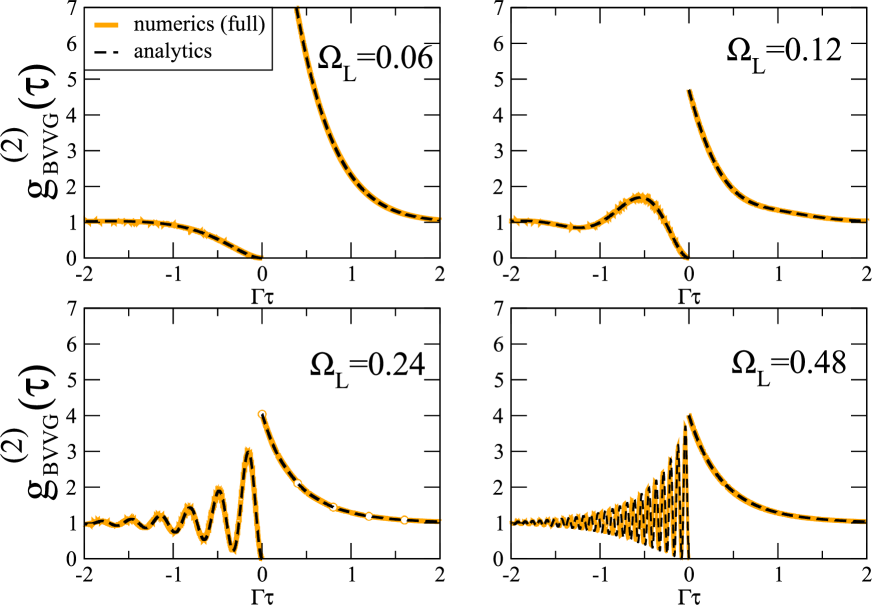
Figure 2: Photon-photon correlations between exciton and biexciton photons for different driving strengths $\Omega_{L}[\text{ps}^{-1}]$ with $\Gamma=0.002\text{ps}^{-1}$ and $\Delta=3.0\text{ps}^{-1}$. The numerical solution is derived from the complete master equation. The analytical solutions are given in the text in the adiabatic limt. For moderate driving strength the agreement is very good.

So, to calculate the two-time correlation function, one needs the steady state value of $\rho_{ii}(\infty)$ and the time-dynamics of $\rho^{jj}_{kk}(\tau)$ with the initial condition of $\rho^{jj}_{kk}(0)=|\langle k||j\rangle|^{2}$. To be explicit, for the biexciton-exciton correlation, we have $i=B,j=V,k=V,l=G$. Therefore, the observable can be expressed as:

$$g^{(2)}_{BVVG}(\tau)= \lim\limits_{t\to\infty}\frac{\boldsymbol{\big{\langle}}c^{\dagger}_{BV}(t)c^{\dagger}_{VG}(t+\tau)c^{\phantom{\dagger}}_{GV}(t+\tau)c^{\phantom{\dagger}}_{VB}(t)\boldsymbol{\big{\rangle}}}{\boldsymbol{\big{\langle}}c^{\dagger}_{BV}(t)c^{\phantom{\dagger}}_{VB}(t)\boldsymbol{\big{\rangle}}\boldsymbol{\big{\langle}}c^{\dagger}_{VG}(t)c^{\phantom{\dagger}}_{GV}(t)\boldsymbol{\big{\rangle}}}=\frac{\rho_{BB}(\infty)\rho^{VV}_{VV}(\tau)}{\rho_{BB}(\infty)\rho_{VV}(\infty)}=\frac{\rho^{VV}_{VV}(\tau)}{\rho_{VV}(\infty)}.$$ (30)

So, we just need the steady state values, and the dynamics for the $V-$exciton state with the initial conditions of $\rho_{VV}=1$. The exciton dynamics reads:

$$\rho^{VV}_{VV}(\tau)= \frac{1}{2}e^{-\Gamma\tau}\left[1+\frac{\Omega^{2}}{\Omega^{2}+\Gamma^{2}}\left(\cosh(\Gamma\tau)+\frac{\Gamma^{2}}{\Omega^{2}}\cos(\Omega\tau)\right)\right].$$ (31)

with the steady state $\rho^{VV}_{VV}(\infty)=(\Omega/2)^{2}/(\Omega^{2}+\Gamma^{2})$, approximately $1/4$ in the strong driving limit. The measured correlation, when the biexciton photon is detected first, reads:

$$g^{(2)}_{BVVG}(\tau)= \frac{\rho^{VV}_{VV}(\tau)}{\rho_{VV}(\infty)}=2e^{-\Gamma\tau}\left(1+\cosh(\Gamma\tau)+\alpha[1+\cos(\Omega\tau)]\right),$$ (32)

with $\alpha=\Gamma^{2}/\Omega^{2}$. In the long-time limit, the correlation always converges to $1$, as it should be. This can be seen, by taking into account, that $\cosh(\Gamma\tau)=[\exp(\Gamma\tau)+\exp(-\Gamma\tau)]/2$. Furthermore, the correlation starts always with

$$g^{(2)}_{BVVG}(0)= 4\left(1+\alpha\right),$$ (33)

which reaches $4$ in the strong driving limit, i.e. $\alpha\rightarrow 0$. The correlation cannot start with a smaller value. For weaker driving, the initial correlation can be arbitrary high with $\alpha\gg 1$. The correlation function therefore always resides between $4<g^{(2)}_{BVVG}(0)<\infty$. This corresponds to the physical intuition, that the probability to measure an exciton photon is dramatically higher if a biexciton photon is detected. The opposite is the case, if the exciton photon is measured first. This is the next case, we are now considering.

If the exciton photon is detected first, then the correlation has the following index set $i=V,j=G,k=B,l=V$ with the observable of

$$g^{(2)}_{VGGB}(\tau)= \lim\limits_{t\to\infty}\frac{\boldsymbol{\big{\langle}}c^{\dagger}_{VG}(t)c^{\dagger}_{BV}(t+\tau)c^{\phantom{\dagger}}_{VB}(t+\tau)c^{\phantom{\dagger}}_{GV}(t)\boldsymbol{\big{\rangle}}}{\boldsymbol{\big{\langle}}c^{\dagger}_{VG}(t)c^{\phantom{\dagger}}_{GV}(t)\boldsymbol{\big{\rangle}}\boldsymbol{\big{\langle}}c^{\dagger}_{BV}(t)c^{\phantom{\dagger}}_{VB}(t)\boldsymbol{\big{\rangle}}}=\frac{\rho_{VV}(\infty)\rho^{GG}_{BB}(\tau)}{\rho_{BB}(\infty)\rho_{VV}(\infty)}=\frac{\rho^{GG}_{BB}(\tau)}{\rho_{BB}(\infty)}.$$ (34)

For this sequence of detection events, the biexciton population dynamics needs to be calculated with following initial conditions $B(t)=0$, $\rho^{GG}_{BB}(0)=0$ and $D(t)=-1$. The solution is

$$\rho^{GG}_{BB}(t)= \frac{e^{-\Gamma t}\Omega^{2}}{2(\Omega^{2}+\Gamma^{2})}\left[\sinh(\Gamma t)-\cos(\Omega t)+e^{-\Gamma t}\right]=\frac{e^{-\Gamma t}\Omega^{2}}{2(\Omega^{2}+\Gamma^{2})}\left[\cosh(\Gamma t)-\cos(\Omega t)\right]$$ (35)

with the steady state $\rho^{GG}_{BB}(\infty)=(\Omega/2)^{2}/(\Omega^{2}+\Gamma^{2})$, and the corresponding normalized correlation function reads:

$$g^{(2)}_{VGGB}(\tau)= 2e^{-\Gamma\tau}\left[\cosh(\Gamma\tau)-\cos(\Omega\tau)\right]=1+e^{-\Gamma\tau}\left(e^{-\Gamma\tau}-2\cos(\Omega\tau)\right).$$ (36)

This correlation always starts with $g^{(2)}_{VGGB}(0)=0$, i.e. it takes always a finite time to detect after an exciton a biexciton photon. The long time limit is $g^{(2)}_{VGGB}(\infty)=1$. Furthermore, the maximum of the correlation can be inferred from $\exp(-\Gamma\tau)\approx 1$ and a driving amplitude chosen such that $\cos(\Omega\tau)=-1$, then $g^{(2)}_{GVVB}(\tau)<4$. So, the exciton-biexciton correlations oscillates between $0\leq g^{(2)}_{GVVB}(\tau)<4$.

In Fig. 2, the numerical and analytical solutions of the photon correlation function between the detection of the biexciton and exciton and vice versa is plotted. Note, $g^{(2)}_{GVVB}(\tau)=g^{(2)}_{BVVG}(-\tau)$. The numerical solution (black, dashed line) is obtained by evaluation of the full density matrix equation without any further approximation than necessary to obtain the master equation in Eq. (3). The analytical solutions of Eq. (32) and (36) (orange, solid line) agrees well in this driving limit: $\Omega_{L}\ll\Delta$. Numerical evaluations show that the approximations for the analytical solutions hold up to an acceptable mistake until $\Omega_{L}\leq\Delta/3$ for the exciton-biexciton direction $\tau<0$. For $\tau>0$, the dynamics is for strong driving dominated by the dissipative dynamics, as the driving suppresses any oscillations with the factor $\Gamma^{2}/\Omega^{2}$. Since the approximations hold perfectly in the weak driving limit, the solution for $\tau>0$, namely for the biexciton-exciton measurement sequence, holds numerically for every driving, as long as the master equations stays valid.

The plot clearly shows, that a $g^{(2)}(\tau)-$function of smaller than $1$ always shows that an exciton photon is detected first, and in contrast a $g^{(2)}(\tau)-$value of larger than $4$, refers to a biexciton-exciton photon detection order. The driving strength steers a Rabi oscillation signal between the exciton and biexciton detection for $\tau<1$. The stronger the driving, the faster the biexciton photon can be detected. But there is no driving strength, where (theoretically) the $g^{(2)}(\tau)-$ function does not initially start with value of zero. Experimentally, the time resolution may lead to finite values, but always to values smaller than $1$, since the oscillations maximum amplitude is stronger damped than the oscillations minimum rises (biexciton decay versus exciton decay).

4 Dressed states

To enable a vanishing time-ordering, a spectral selection of the photons is necessary. Until now, the calculations have not distinguished between an exciton photon in the strong and weak driving limit. Basically, three photons with slightly different frequencies can be emitted from the exciton, as well as from the biexciton state. To unravel these three possibilities, it is necessary to change the basis of the theoretical description into the dressed state coordinates. In order to investigate the different spectral contributions and the dependence of the time-ordering on the driving strength, we express the dressed states in terms of the bare states and employ the solutions of the previous sections.

To address the dressed states individually, we find the Eigenstates of the Hamiltonian, i.e. the Eigenstates of the coherent evolution only.

$$H_{R}= \Delta(\left|H\right\rangle\left\langle H\right|+\left|V\right\rangle\left\langle V\right|)+\Omega_{L}(\left|G\right\rangle\left\langle H\right|+\left|B\right\rangle\left\langle H\right|+\text{h.a.})\rightarrow\begin{pmatrix}0&\Omega_{L}&0&0\\ \Omega_{L}&\Delta&\Omega_{L}&0\\ 0&\Omega_{L}&0&0\\ 0&0&0&\Delta\end{pmatrix},$$ (37)

ordered in the basis $\left\{|G\rangle,|H\rangle,|B\rangle,|V\rangle\right\}$ and for the case of resonant two-photon driving of the biexciton and a polarization-selective driving of the horizontal exciton level, without affecting the vertical-polarized transitions. The diagonalization results in four Eigenvalues

$$e_{0} =0,\quad e_{1}=\Delta,\quad e_{3}=\frac{1}{2}\left(\Delta+\sqrt{8\Omega^{2}+\Delta^{2}}\right),\quad e_{4}=\frac{1}{2}\left(\Delta-\sqrt{8\Omega^{2}+\Delta^{2}}\right),$$ (38)

with the corresponding Eigenvectors:

$$|+\rangle= \frac{\Omega}{\sqrt{2\Omega^{2}+e^{2}_{3}}}\left(|G\rangle+\frac{e_{3}}{\Omega}|H\rangle+|B\rangle\right),\quad|V\rangle=|V\rangle$$ (39)

$$|-\rangle= \frac{\Omega}{\sqrt{2\Omega^{2}+e_{4}^{2}}}\left(|G\rangle+\frac{e_{4}}{\Omega}|H\rangle+|B\rangle\right),\quad|0\rangle=\frac{1}{\sqrt{2}}\left(|B\rangle-|G\rangle\right).$$ (40)

Orthogonality and normalization can be proven via helpful relation between the eigenvalues, cf. D.

From the Eigenvalues it can be already seen, that the biexciton, the $H-$exciton and the ground state form a superposition due to the coherent driving. The external laser field creates coherences in between these states, which leads to three frequency-differentiated biexciton-exciton transitions $\sigma_{+V},\sigma_{-V},\sigma_{0V}$ and also three exciton-ground state transitions $\sigma_{V+},\sigma_{V-},\sigma_{V0}$. If the driving is weak, the frequencies do not appear as separate peaks for they lie all within the radiative linewidth $\Gamma$. But in the strong driving limit, Mollow physics appear and become spectrally resolved in the spectrum.

There is a particularly interesting feature that becomes visible in the strong driving limit. In contrast to the full exciton-biexciton correlation, where at least in one delay direction, a $g^{(2)}-$value smaller than $1$ always occurs, it is possible to create a signal that never exhibits a $g^{(2)}-$value smaller than one. This is rendered possible via a decay in form of a superposition and is a specific property of the strong driving limit, where the coherences are strongly enhanced. Those superpositions do not differentiate between exciton and biexciton photons anymore. In this case, the time-ordering in the cascade has been lifted. And it is not possible to judge via the $g^{(2)}-$signal whether a biexciton or exciton photon has been measured first. In the following, we calculate analytically the signal of the correlation functions, which exhibits in the strong driving limit such a vanishing time-reordering. The observable reads:

$$g^{(2)}_{+VV+}(\tau)= \lim\limits_{t\to\infty}\frac{\boldsymbol{\big{\langle}}c^{\dagger}_{+V}(t)c^{\dagger}_{V+}(t+\tau)c^{\phantom{\dagger}}_{+V}(t+\tau)c^{\phantom{\dagger}}_{V+}(t)\boldsymbol{\big{\rangle}}}{\boldsymbol{\big{\langle}}c^{\dagger}_{+V}(t)c^{\phantom{\dagger}}_{V+}(t)\boldsymbol{\big{\rangle}}\boldsymbol{\big{\langle}}c^{\dagger}_{V+}(t)c^{\phantom{\dagger}}_{+V}(t)\boldsymbol{\big{\rangle}}}.$$ (41)

The system undergoes the cascade either from $|+\rangle\rightarrow|V\rangle\rightarrow|+\rangle$. This observable will be calculated in the next section, and it will be shown that the $0-$state observable exhibits the same dynamics with

$$g^{(2)}_{0VV0}(\tau)= \lim\limits_{t\to\infty}\frac{\boldsymbol{\big{\langle}}c^{\dagger}_{0V}(t)c^{\dagger}_{V0}(t+\tau)c^{\phantom{\dagger}}_{0V}(t+\tau)c^{\phantom{\dagger}}_{V0}(t)\boldsymbol{\big{\rangle}}}{\boldsymbol{\big{\langle}}c^{\dagger}_{0V}(t)c^{\phantom{\dagger}}_{V0}(t)\boldsymbol{\big{\rangle}}\boldsymbol{\big{\langle}}c^{\dagger}_{V0}(t)c^{\phantom{\dagger}}_{0V}(t)\boldsymbol{\big{\rangle}}}=g^{(2)}_{+VV+}(\tau).$$ (42)

For the experimental signal, in Sec. 6, another correlation function is of importance, i.e. a cross-correlation between the dressed states:

$$g^{(2)}_{+VV0}(\tau)= \lim\limits_{t\to\infty}\frac{\boldsymbol{\big{\langle}}c^{\dagger}_{+V}(t)c^{\dagger}_{V0}(t+\tau)c^{\phantom{\dagger}}_{0V}(t+\tau)c^{\phantom{\dagger}}_{V+}(t)\boldsymbol{\big{\rangle}}}{\boldsymbol{\big{\langle}}c^{\dagger}_{+V}(t)c^{\phantom{\dagger}}_{V+}(t)\boldsymbol{\big{\rangle}}\boldsymbol{\big{\langle}}c^{\dagger}_{V0}(t)c^{\phantom{\dagger}}_{0V}(t)\boldsymbol{\big{\rangle}}}.$$ (43)

Due to intrinsic symmetric reasons in detail explained in E, this cross-correlation stays the same whether first the $0-$state photon and the $+-$state photon is detected or the other way round, expressed in a formula: $g^{(2)}_{+VV0}(\tau)=g^{(2)}_{0VV+}(\tau)$. The $-$state photons are not included in the experimental signal as those photons are too close to the frequency of the laser photons and cannot easily be distinguished from elastic scattering events.

5 Photon-Photon correlation of selected dressed states

The detection sequence is again two-fold, either the $|+\rangle$ or the $|V\rangle$ photon is detected first. The detection is polarized selective, and so the calculation is simplified due to a vanishing $|H\rangle$ contribution. Using the same method as before, we need the correlation with following flip operators for $\tau>0$:

$$g^{(2)}_{+VV+}(\tau)= \lim\limits_{t\to\infty}\frac{\boldsymbol{\big{\langle}}\sigma_{+V}(t)\sigma_{V+}(t+\tau)\sigma_{+V}(t+\tau)\sigma_{V+}(t)\boldsymbol{\big{\rangle}}}{\boldsymbol{\big{\langle}}\sigma_{++}(t)\boldsymbol{\big{\rangle}}\boldsymbol{\big{\langle}}\sigma_{VV}(t)\boldsymbol{\big{\rangle}}}$$

Therefore, the observable can be expressed as:

$$g^{(2)}_{+VV+}(\tau)= \frac{\rho_{++}(\infty)\rho^{VV}_{VV}(\tau)}{\rho_{++}(\infty)\rho_{VV}(\infty)}=2e^{-\Gamma\tau}\left(1+\cosh(\Gamma\tau)+\alpha[1+\cos(\Omega\tau)]\right).$$ (44)

This part of the correlation has not change in comparison to the previous calculation. This is due to the fact, that the conditional probablity of the $V-$exciton state is measured, and this state does not change with the driving strength, for it is decoupled from the laser. However, for $\tau<0$, the correlation function reads:

$$g^{(2)}_{V++V}(\tau)= \frac{\rho_{VV}(\infty)\rho^{++}_{++}(\tau)}{\rho_{VV}(\infty)\rho_{++}(\infty)}=\frac{\rho^{++}_{++}(\tau)}{\rho_{++}(\infty)}.$$ (45)

We need to express the dressed state basis in terms of the bare state to use the aforementioned solution. Under the condition, that the horizontal-polarized photons are not detected, the corresponding dressed state reads:

$$|+\rangle= \frac{1}{\sqrt{2}}\left(|G\rangle+|B\rangle\right).$$ (46)

Now, the density matrix dynamics needs to be expressed in terms of this superposition:

$$g^{(2)}_{V++V}(\tau)= \text{Tr}\left[\left|+\right\rangle\left\langle+\right|\frac{\sigma_{++}(\tau)}{\rho_{++}(\infty)}\right]=\text{Tr}\left[\left(\left|B\right\rangle\left\langle B\right|+\left|B\right\rangle\left\langle G\right|+\left|G\right\rangle\left\langle B\right|+\left|G\right\rangle\left\langle G\right|\right)\frac{\sigma_{++}(\tau)}{2\rho_{++}(\infty)}\right].$$

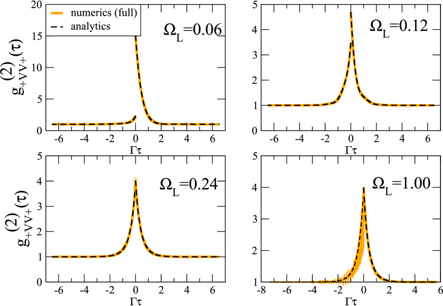
Figure 3: Photon-photon correlations between $+$ biexciton and $+$ exciton photon for different driving strengths $\Omega_{L}[\text{ps}^{-1}]$ with $\Gamma=0.002\text{ps}^{-1}$ and $\Delta=3.0\text{ps}^{-1}$. The numerical solution is derived from the complete master equation. The analytical solutions are given in the text in the adiabatic limt. For moderate driving strength the agreement is very good.

Due to the superposition, the calculation can be more tedious than before, if done separately. However, it is more feasible to calculate the dynamics directly via a superpostion of the initial conditions. After measuring a $V-$photon, the system is in the following mixture of states: $\rho^{++}(0)=\left(\left|B\right\rangle\left\langle B\right|+\left|B\right\rangle\left\langle G\right|+\left|G\right\rangle\left\langle B\right|+\left|G\right\rangle\left\langle G\right|\right)/2$. Therefore, the initial conditions read:

$$D^{++}_{0} :=\rho^{++}_{BB}-\rho^{++}_{GG}=0$$ (47)

$$B^{++}_{0} :=\rho^{++}_{BG}-\rho^{++}_{GG}=0$$ (48)

$$\Sigma^{++}_{0} :=\rho^{++}_{BB}+\rho^{++}_{VV}+\rho^{++}_{HH}+\rho^{++}_{GG}=2.$$ (49)

The correlation itself reads with its corresponding initial condition:

$$\boldsymbol{\big{\langle}}\sigma_{++}(\tau)\boldsymbol{\big{\rangle}}|_{\rho^{++}(0)}= \frac{1}{4}\left(\rho^{++}_{BB}(\tau)+\rho^{++}_{GG}(\tau)+2\text{Re}\left[\rho^{++}_{GB}(\tau)\right]\right).$$ (50)

Given all the initial conditions, the correlation can easily be computed, cf. E, and reads:

$$g^{(2)}_{V++V}(\tau)= 1+2\frac{1+\alpha}{1+2\alpha}\left[e^{-2\Gamma\tau}\left(1-\frac{1}{2}\frac{1}{1+\alpha}\right)+e^{-\Gamma\tau}\left(1-\frac{\alpha\cos(\Omega\tau)}{1+\alpha}\right)\right],$$ (51)

with $\alpha:=\Gamma^{2}/\Omega^{2}$. This formula constitutes the main result of this paper. In Fig. 3, the full numerical solution without adiabatic approximation (solid, orange line) is compared with the analytical formula (dashed, black line) given in Eq. (44) and (51). The results agree and confirm the analytical calculation up to driving strength $\Omega_{L}<\Delta/3$. For very strong driving, fast oscillations appear below the adiabatic curve, see Fig. 3 (lower right panel). In this limit, the fast oscillations between the exciton states lead even to values of below $1$. However, the initial value of the correlations functions is always larger than $1$, as the analytical formula shows:

$$g^{(2)}_{V++V}(0) =4\frac{1+\alpha}{1+2\alpha}.$$ (52)

So, for large driving compared to the decay constant, i.e. $\alpha\rightarrow 0$, the initial value approaches $g^{(2)}_{V++V}(0)\rightarrow 4$, showing exactly the time-reordering reversal. The detection schemes are not distinguishable anymore, since $g^{(2)}_{V++V}(0)\approx g^{(2)}_{+VV+}(0)$ is valid. This is the specific result of such a two-photon driving and frequency-polarization filtered detection setup. In the low excitation regime $\alpha\gg 1$ , it can be seen that the minimum of the correlation function is $2$. Investigating the total maximum of the correlation by assuming $\cos(\Omega\tau)=-1$, the correlation in the adiabatic regime stays with the interval $2<g^{(2)}_{V++V}(0)<4$. All these properties can be seen in the Fig. 3 for the different driving strength.

The cross-correlation between the dressed states read:

$$g^{(2)}_{+VV0}(\tau)= \lim\limits_{t\to\infty}\frac{\boldsymbol{\big{\langle}}\sigma_{+V}(t)\sigma_{V0}(t+\tau)\sigma_{0V}(t+\tau)\sigma_{V+}(t)\boldsymbol{\big{\rangle}}}{\boldsymbol{\big{\langle}}\sigma_{++}(t)\boldsymbol{\big{\rangle}}\boldsymbol{\big{\langle}}\sigma_{VV}(t)\boldsymbol{\big{\rangle}}}=\frac{\rho_{++}(\infty)\rho^{VV}_{VV}(\tau)}{\rho_{++}(\infty)\rho_{VV}(\infty)}=\frac{\rho^{VV}_{VV}(\tau)}{\rho_{VV}(\infty)},$$

which we have already calculated. However, the inverted correlation cannot be expressed with the derived results from before, see for details E:

$$g^{(2)}_{V0+V}(\tau)= \lim\limits_{t\to\infty}\frac{\boldsymbol{\big{\langle}}\sigma_{V0}(t)\sigma_{+V}(t+\tau)\sigma_{V+}(t+\tau)\sigma_{0V}(t)\boldsymbol{\big{\rangle}}}{\boldsymbol{\big{\langle}}\sigma_{++}(t)\boldsymbol{\big{\rangle}}\boldsymbol{\big{\langle}}\sigma_{VV}(t)\boldsymbol{\big{\rangle}}}=\frac{\rho^{00}_{++}(\tau)}{\rho_{++}(\infty)}.$$ (53)

The solution differs just in one sign and reads:

$$g^{(2)}_{V+0V}(\tau)= 1+2\frac{1+\alpha}{1+2\alpha}\left[e^{-2\Gamma\tau}\left(1-\frac{1}{2}\frac{1}{1+\alpha}\right)-e^{-\Gamma\tau}\left(1+\frac{\alpha\cos(\Omega\tau)}{1+\alpha}\right)\right]$$ (54)

$$= 1+\frac{1}{1+2\alpha}\left[e^{-2\Gamma\tau}\left(1+2\alpha\right)-2e^{-\Gamma\tau}\left(1+\alpha+\alpha\cos(\Omega\tau)\right)\right].$$ (55)

In contrast to the other dressed correlation in this section, this one starts always with $0$ for $\tau<0$, cf. Fig. 4.

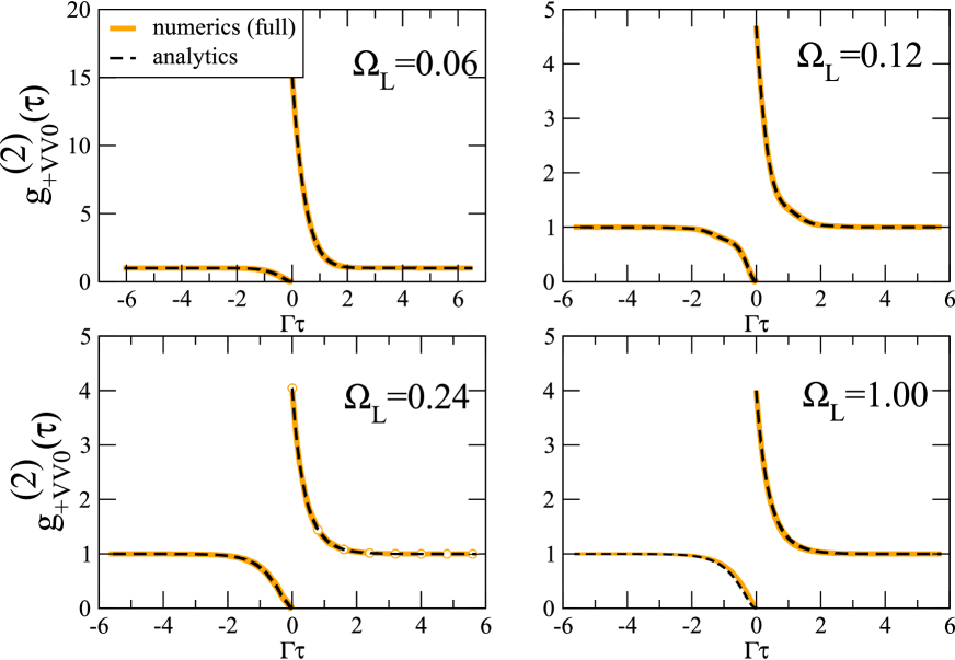
Figure 4: Photon-photon correlations between $+$ and $0$-state photons for different driving strengths $\Omega_{L}[\text{ps}^{-1}]$ with $\Gamma=0.002\text{ps}^{-1}$ and $\Delta=3.0\text{ps}^{-1}$. The numerical solution is derived from the complete master equation. The analytical solutions are given in the text in the adiabatic limt. For moderate driving strength the agreement is very good.

The antibunching feature is independent of the driving strength. The bunching on the biexciton-exciton side $\tau>0$ is however decreased for stronger driving and the numerical and analytical solutions agree well.

With the symmetries at hand, we can now turn to the experimental data for different intensities and compare the theoretical findings with the experiments.

6 Comparison with the experiment

In the experiment, the biexciton-exciton correlation is taken only partially. The contribution from the $|-\rangle$-state are difficult to distinguish from the laser photons and are therefore excluded from the detection setup. So, the biexciton-exciton correlation reads in the experiment:

$$g^{(2)}_{\text{EX}}(\tau)= \frac{1}{4}\left(g^{(2)}_{\text{+VV+}}(\tau)+g^{(2)}_{\text{0VV0}}(\tau)+g^{(2)}_{\text{+VV0}}(\tau)+g^{(2)}_{\text{0VV+}}(\tau)\right),$$ (56)

which are all possible detection events for this chosen frequency-window. We take advantage of our definition: $g^{(2)}_{\text{ijkl}}(\tau)=\rho^{jj}_{kk}(\tau)/\rho^{jj}_{kk}(\infty)$, i.e. the correlation describes the conditional probability to measure the photon from state $|k\rangle$, after a photon is detected, which collapses the state of the system to the state $|j\rangle$. Using this definition, we can write the biexciton-exciton detection sequence as:

$$g^{(2)}_{\text{EX}}(\tau)= \frac{\rho^{VV}_{VV}(\tau)}{\rho^{VV}_{VV}(\infty)}=3+e^{-2\Gamma\tau}+2\alpha e^{-\Gamma\tau}[1+\cos(\Omega\tau)].$$ (57)

However, the exciton-biexciton direction is more complicated. All possible detection events read:

$$g^{(2)}_{\text{EX}}(\tau)= \frac{1}{4}\left(g^{(2)}_{\text{V++V}}(\tau)+g^{(2)}_{\text{V00V}}(\tau)+g^{(2)}_{\text{V+0V}}(\tau)+g^{(2)}_{\text{V0+V}}(\tau)\right),$$ (58)

but we know, out of symmetry reasons that $\rho^{++}_{++}(\tau)=\rho^{00}_{00}(\tau)$ and $\rho^{++}_{00}(\tau)=\rho^{00}_{++}(\tau)$. Therefore, we can write:

$$g^{(2)}_{\text{EX}}(\tau)= \frac{1}{2}\left(\frac{\rho^{++}_{++}(\tau)}{\rho^{++}_{++}(\infty)}+\frac{\rho^{++}_{00}(\tau)}{\rho^{++}_{00}(\infty)}\right)=1+e^{-2\Gamma\tau}-\frac{2\alpha\cos(\Omega\tau)}{1+2\alpha}e^{-\Gamma\tau},$$ (59)

so for $\tau\rightarrow 0$, the conditional probability reads

$$g^{(2)}_{\text{EX}}(0)= 1+1-\frac{2\alpha}{1+2\alpha}=2-\frac{2\alpha+1-1}{1+2\alpha}=1+\frac{1}{1+2\alpha}>1.$$ (60)

Both detection sequences show bunching. In Fig. 5(a), the bunching effect is shown in the experimental data for the strong (green) and weak driving regime (orange). For stronger excitation the detection around $\tau=0$ symmetrizes, which signifies a superposition in detection events rendering the detection order partially indistinguishable. However, in contrast to the case of $g^{(2)}_{\text{+VV+}}(\tau)$ correlation function, the peak around $\tau=0$ cannot be completely symmetrical due to antibunching contribution from the cross-correlation, e.g. $g^{(2)}_{\text{+VV0}}(\tau)$. The analytical theory reproduces the effect well, cf. Fig. 5(b). Note, the theory is not convoluted with the detector-response function, as the focus of this work is to provide general formulas for the correlation functions and not to discuss detailed experimental data. In consequence, the comparison to the experiment is only qualitatively without fitting the decay and excitation constant properly.

Nevertheless, the theory reproduces the important fact, that antibunching is highly unlikely in this dectection setup. For antibunching is created in a superposition state of all occuring dressed state emission events, locked, phase-matched to the exciton-emisson. The signal is not just a sum of the correlation functions but a constructive and destructive interference between photon detections. Leading to the conclusion, that it is much harder in this setup to render the antibunching visible out of the aforementioned reasons.

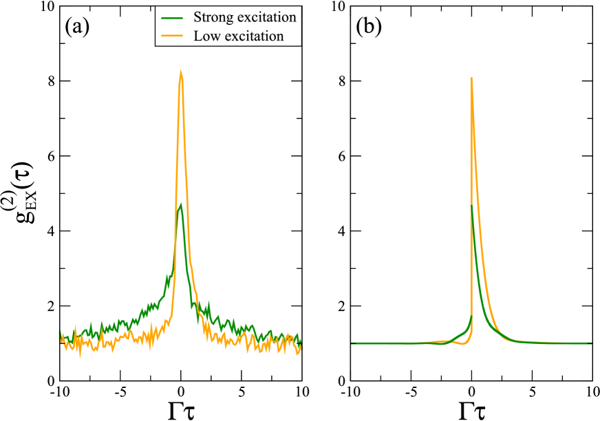
Figure 5: Comparison between experiment (a) and theory (b) for two low $(30\mu\text{W})$ and strong excitation $(100\mu\text{W})$ power and the exciton-biexciton photon-photon correlations without $|-\rangle$ state contributions. The qualitative agreement is very good. Both plots show the symmetrization of detection events for stronger excitation (green) in comparison to lower excitation (orange). The experimental data is shown with a substracted background, in particular for the lower excitation.

7 Conclusion

We have calculated analytically the two-time correlations of the exciton-biexciton cascade in the adiabatic limit, where the detuning between the laser and the excitonic transition is much larger than the driving amplitude. In this limit, we discussed the correlation of the biexciton- exciton photons, which showed clearly a time-reordering. It is always possible to distinguish the detection sequence by their $g^{(2)}_{BVVG}(\tau)$ values around zero $-1/\Gamma\ll\tau\ll 1/\Gamma$, i.e. $g^{(2)}(\tau)_{BVVG}>1$ the biexciton has been detected, then the exciton, and $g^{(2)}_{XB}(\tau)<1$ vice versa. If the dressed states can spectrally be selected, it is possible to erase this time-ordering. We showed this analytically by calculating the correlation function in the dressed state basis $g^{(2)}_{+VV+}(\tau)$. Furthermore, we showed with our calculations the limits of the correlation functions in the idealized situation of an isolated four level system, and why it is difficult to observe in such a system the antibunching effect.

The research leading to these results has received funding from the European Research Council (ERC) under the European Union’s Seventh Framework ERC Grant Agreement No. 615613 and from the German Research Foundation (DFG) through SFB 787 via Projects No. RE2974/4-1 and No. RE2974/12-1. A.C. gratefully acknowledges support from the SFB 910: “Control of self-organizing nonlinear systems.“

Appendix A Comparison to the two-level case

In this section, we show that the resonant two-photon driven four-level system obeys the well-known two-level physics. The resonant Mollow problem is cast into the following master equation:

$$\dot{\rho}= -i\left[\Omega_{2}(\left|G\right\rangle\left\langle B\right|+\left|B\right\rangle\left\langle G\right|),\rho\right]+\Gamma_{2}\mathcal{D}[\sigma_{GB}]\rho,$$ (61)

using the standard Lindblad form $\mathcal{D}[J]\rho=2J\rho J^{\dagger}-\{J^{\dagger}J,\rho\}$ and denoting the parameter with ₂ to distinguish them from the four-level case. Using the master equation, the follow set of differential equations of motion is yield with $\rho_{ij}=\langle i|\rho|j\rangle$:

$$\dot{\rho}_{GG}= 2\Gamma_{2}\rho_{BB}+i\Omega_{2}\left(\rho_{BG}-\rho_{GB}\right)=2\Gamma_{2}(\Sigma_{2,0}-\rho_{GG})+i\Omega_{2}\left(\rho_{BG}-\rho_{GB}\right),$$ (62)

$$\dot{\rho}_{BG}= -\Gamma_{2}\rho_{BG}-i\Omega_{2}\left(\rho_{BB}-\rho_{GG}\right),$$ (63)

$$\dot{\rho}_{BB}= -2\Gamma_{2}\rho_{BB}-i\Omega_{2}\left(\rho_{BG}-\rho_{GB}\right),$$ (64)

where we used again $\rho_{BB}+\rho_{GG}=\Sigma_{2,0}$ with typically $\Sigma_{2}(t=0)=\Sigma_{2,0}=1$. We substract the population dynamics from each other and also the polarization dynamics: $D(t):=\rho_{BB}(t)-\rho_{GG}(t)$ and the linear independent imaginary part of the polarization between both states $B(t):=\rho_{BG}(t)-\rho_{GB}(t)$:

$$\dot{B}(t)= -\Gamma_{2}\rho_{BG}+\Gamma_{2}\rho_{GB}-i2\Omega_{2}\left(\rho_{BB}-\rho_{GG}\right)=-\Gamma_{2}B(t)-i2\Omega_{2}D(t),$$

$$\dot{D}(t)= -2\Gamma_{2}\rho_{BB}-2\Gamma_{2}(\Sigma_{2,0}-\rho_{GG})-i2\Omega_{2}\left(\rho_{BG}-\rho_{GB}\right)=-2\Gamma_{2}\left(D(t)+\Sigma_{2,0}\right)-i2\Omega_{2}B(t).$$

This is exactly the same set of equation of motions as the adabiatic version of the two-photon biexciton driving case. The difference is hidden in $\Sigma_{2,0}\neq\Sigma_{0}$ in the main text. The dynamics of the exciton level play a role and allow different values. Furthermore, the transition operator $\sigma_{GB}$ does not correspond to a single-photon emission but in this case to a two-photon emission process. However, the well-known solution of the Mollow problem apply to the four-level case in the adiabatic limit, also, but it needs to be unraveled in terms of single-photon detection events.

Appendix B Laplace solution

In this section, the analytical solution of the inversion and transition amplitude dynamics are derived. The problem is identical to the dynamics of a two-level system but with a different dissipative dynamics underlying. For completeness, we derive the solution via Lapace transformation. In text books, mainly a diagonalization technique is applied [2]. We transform Eq. (16) and  (17) the into the Laplace domain with $\Sigma_{0}=\rho_{GG}(0)+\rho_{BB}(0)+\rho_{VV}(0)+\rho_{HH}(0)$:

$$s\bar{D}-D(0)= -\Gamma\bar{D}-\Gamma\frac{\Sigma_{0}}{s}-i\Omega\bar{B}$$ (65)

$$s\bar{B}-B(0)= -\Gamma\bar{B}-i\Omega\bar{D}.$$ (66)

Let’s solve this, and abbreviate $B(0)=B_{0}$ and $D(0)=D_{0}$. We see that:

$$\bar{B}= \frac{B_{0}}{s+\Gamma}-i\Omega\frac{\bar{D}}{s+\Gamma}$$ (67)

We insert this solution into the equation for the inversion:

$$s\bar{D}-D_{0}= -\Gamma\bar{D}-\Sigma_{0}\frac{\Gamma}{s}-i\Omega\left(\frac{B_{0}}{s+\Gamma}-i\Omega\frac{\bar{D}}{s+\Gamma}\right)$$ (68)

$$s\bar{D}= D_{0}-\Gamma\bar{D}-\Sigma_{0}\frac{\Gamma}{s}-i\Omega\frac{B_{0}}{s+\Gamma}-\Omega^{2}\frac{\bar{D}}{s+\Gamma}$$ (69)

$$\bar{D}= D_{0}\frac{(s+\Gamma)}{(s+\Gamma)^{2}+\Omega^{2}}-i\Omega B_{0}\frac{1}{(s+\Gamma)^{2}+\Omega^{2}}-\Sigma_{0}\frac{\Gamma}{s}\frac{s+\Gamma}{(s+\Gamma)^{2}+\Omega^{2}}$$ (70)

and for the polarisation:

$$\bar{B}= \frac{B_{0}}{s+\Gamma}-\frac{i\Omega\bar{D}}{s+\Gamma}=\frac{B_{0}(s+\Gamma)}{(s+\Gamma)^{2}+\Omega^{2}}-i\Omega D_{0}\frac{i\Omega D_{0}}{(s+\Gamma)^{2}+\Omega^{2}}+\frac{\Gamma}{s}\frac{\Sigma_{0}i\Omega}{(s+\Gamma)^{2}+\Omega^{2}}.$$ (71)

We use following Laplace transform identities:

$$\bar{f}(s)=\frac{1}{(s+\Gamma)^{2}+\Omega^{2}}\longrightarrow f(t)=\frac{1}{\Omega}e^{-\Gamma t}\sin(\Omega t)$$ (72)

$$\bar{f}(s)=\frac{s+\Gamma}{(s+\Gamma)^{2}+\Omega^{2}}\longrightarrow f(t)=e^{-\Gamma t}\cos(\Omega t)$$ (73)

$$\bar{f}(s)=\frac{1}{s}\frac{1}{(s+\Gamma)^{2}+\Omega^{2}}\longrightarrow f(t)=\frac{1}{\Omega^{2}+\Gamma^{2}}-\frac{e^{-\Gamma t}}{\Omega}\frac{\Omega\cos(\Omega t)+\Gamma\sin(\Omega t)}{\Omega^{2}+\Gamma^{2}}$$

$$\bar{f}(s)=\frac{1}{s}\frac{s+\Gamma}{(s+\Gamma)^{2}+\Omega^{2}}\longrightarrow f(t)=\frac{\Gamma}{\Omega^{2}+\Gamma^{2}}+e^{-\Gamma t}\ \frac{\Omega\sin(\Omega t)-\Gamma\cos(\Omega t)}{\Omega^{2}+\Gamma^{2}}$$ (74)

In the time domain, the inversion dynamics read

$$D(t)= D_{0}e^{-\Gamma t}\cos(\Omega t)-iB_{0}e^{-\Gamma t}\sin(\Omega t)$$ (75)

$$-\Sigma_{0}\Gamma\left[\Gamma_{n}+e^{-\Gamma t}\ \left(\Omega_{n}\sin(\Omega t)-\Gamma_{n}\cos(\Omega t)\right)\right]$$ (76)

which fulfills: $D(t=0)=D_{0}$ with abbreviated normalized constants

$$\Omega_{n}= \frac{\Omega}{\Omega^{2}+\Gamma^{2}}\qquad\Gamma_{n}=\frac{\Gamma}{\Omega^{2}+\Gamma^{2}}.$$ (77)

The general equation of polarisation reads:

$$B(t)= B_{0}\ e^{-\Gamma t}\cos(\Omega t)-iD_{0}\ e^{-\Gamma t}\sin(\Omega t)$$ (78)

$$+\Sigma_{0}i\Gamma\left[\Omega_{n}-e^{-\Gamma t}\left(\Omega_{n}\cos(\Omega t)+\Gamma_{n}\sin(\Omega t)\right)\right].$$ (79)

Given the initial conditions and the probability conservation, the dynamics of all other quantities can be calculated from these two solutions.

Appendix C Explicit solution of the biexciton dynamics

To derive the solution for the biexciton dynamics, we need to use the transition dynamics $B(t)$ and integrate its equation of motion. As we know the equation of motion of the biexciton density, we yield:

$$\dot{\rho}_{BB}= -2\Gamma\rho_{BB}+\Omega\text{Im}\left[\rho_{BG}\right]=-2\Gamma\rho_{BB}+\frac{\Omega}{2i}\left[\rho_{BG}-\rho_{GB}\right]=-2\Gamma\rho_{BB}+\frac{\Omega}{2i}B(t).$$ (80)

So we can write

$$\rho_{BB}(t)= \rho_{BB}(0)e^{-2\Gamma t}+\frac{\Omega}{2}\rho^{I}_{BB}(t).$$ (81)

with the inhomogeneous solution, that we need to calculate

$$\rho^{I}_{BB}= e^{-2\Gamma t}\int_{0}^{t}dt_{1}e^{2\Gamma t_{1}}2\text{Im}\left[\rho_{BG}\right]=-ie^{-2\Gamma t}\int_{0}^{t}dt_{1}e^{2\Gamma t_{1}}\ B(t_{1})$$ (82)

$$= -i\left(B_{0}-\Sigma_{0}i\Gamma\Omega_{n}\right)e^{-2\Gamma t}\text{Re}\left[\int_{0}^{t}dt_{1}e^{(\Gamma+i\Omega)t_{1}}\ \right]$$ (83)

$$-\left(\Sigma_{0}\Gamma\Gamma_{n}+D_{0}\right)e^{-2\Gamma t}\text{Im}\left[\int_{0}^{t}dt_{1}e^{(\Gamma+i\Omega)t_{1}}\ \right]+\Sigma_{0}\Gamma\Omega_{n}\frac{1-e^{-2\Gamma t}}{2\Gamma}.$$ (84)

The integrals are evaluated:

$$\rho^{I}_{BB}(t)= -i\left(B_{0}-i\Sigma_{0}\Gamma\Omega_{n}\right)e^{-2\Gamma t}\text{Re}\left[\frac{\Gamma-i\Omega}{\Omega^{2}+\Gamma^{2}}\left(e^{(\Gamma+i\Omega)t}-1\right)\right]$$

$$-\left(\Sigma_{0}\Gamma\Gamma_{n}+D_{0}\right)e^{-2\Gamma t}\text{Im}\left[\frac{\Gamma-i\Omega}{\Omega^{2}+\Gamma^{2}}\left(e^{(\Gamma+i\Omega)t}-1\right)\right]+\Sigma_{0}\Gamma\Omega_{n}\frac{1-e^{-2\Gamma t}}{2\Gamma}.$$ (85)

Using

$$\text{Re}\left[(\Gamma-i\Omega)(e^{i\Omega t}-e^{-\Gamma t})\right]= \Gamma\cos(\Omega t)+\Omega\sin(\Omega t)-\Gamma e^{-\Gamma t}$$ (86)

$$\text{Im}\left[(\Gamma-i\Omega)(e^{i\Omega t}-e^{-\Gamma t})\right]= \Gamma\sin(\Omega t)-\Omega\cos(\Omega t)+\Omega e^{-\Gamma t},$$ (87)

we yield for the inhomogeneous solution:

$$\rho^{I}_{BB}(t)= -iB_{0}e^{-\Gamma t}\left[\Gamma_{n}\cos(\Omega t)+\Omega_{n}\sin(\Omega t)-\Gamma_{n}e^{-\Gamma t}\right]$$ (88)

$$-D_{0}e^{-\Gamma t}\left[\Gamma_{n}\sin(\Omega t)-\Omega_{n}\cos(\Omega t)+\Omega_{n}e^{-\Gamma t}\right]$$ (89)

$$+\Sigma_{0}e^{-\Gamma t}\left[\Omega_{n}\sinh(\Gamma t)-\Gamma_{n}\sin(\Omega t)\right].$$ (90)

The complete solution is now given via:

$$\rho_{BB}(t)= \rho_{BB}(0)e^{-2\Gamma t}+-iB_{0}\frac{\Omega}{2}e^{-\Gamma t}\left[\Gamma_{n}\cos(\Omega t)+\Omega_{n}\sin(\Omega t)-\Gamma_{n}e^{-\Gamma t}\right]$$ (91)

$$-D_{0}\frac{\Omega}{2}e^{-\Gamma t}\left[\Gamma_{n}\sin(\Omega t)-\Omega_{n}\cos(\Omega t)+\Omega_{n}e^{-\Gamma t}\right]$$ (92)

$$+\Sigma_{0}\frac{\Omega}{2}e^{-\Gamma t}\left[\Omega_{n}\sinh(\Gamma t)-\Gamma_{n}\sin(\Omega t)\right].$$ (93)

With the biexciton dynamics given, all other excitonic dynamics can be directly calculated, using the relation given by the symmetries of the full set of equation of motion in Eq. (3).

Appendix D Convenient relations of the dressed state normalization factors

We define following normalization factors:

$$a_{1}=\frac{\Omega}{\sqrt{2\Omega^{2}+e^{2}_{3}}},\qquad a_{2}=\frac{\Omega}{\sqrt{2\Omega^{2}+e^{2}_{4}}},\qquad\text{and}\qquad a_{3}=\frac{1}{\sqrt{2}}.$$ (94)

with

$$e_{3}= \frac{1}{2}\left(\Delta+\sqrt{8\Omega^{2}+\Delta^{2}}\right),\qquad e_{4}=\frac{1}{2}\left(\Delta-\sqrt{8\Omega^{2}+\Delta^{2}}\right).$$ (95)

For example:

$$e_{3}e_{4}= \frac{1}{4}\left(\Delta^{2}-8\Omega^{2}-\Delta^{2}\right)=-2\Omega^{2}.$$ (96)

And,

$$a_{1}^{2}+a_{2}^{2}= \frac{1}{2}$$ (97)

$$a^{2}_{1}\Delta_{+}+a^{2}_{2}\Delta_{-} =0$$ (98)

$$a^{2}_{1}\Delta_{-}+a^{2}_{2}\Delta_{+} =\frac{\Delta}{2}.$$ (99)

Just for convenience some more interesting algebraic relations:

$$\frac{1}{2}\frac{e_{3}}{e_{3}-e_{4}}= a_{2}^{2}$$ (100)

$$\frac{1}{2}\frac{e_{4}}{e_{4}-e_{3}}= a_{1}^{2}.$$ (101)

With these algebraic relations, orthogonality and orthonormalization can easily be shown.

Appendix E Dressed correlation calculation

Here, we calculate the dynamics of the $+$-state photon, which depends on the following population dynamics:

$$\rho^{++}_{++}(\tau):=\boldsymbol{\big{\langle}}\sigma_{++}(\tau)\boldsymbol{\big{\rangle}}|_{\rho^{++}(0)}= \frac{1}{4}\left(\rho^{++}_{BB}(\tau)+\rho^{++}_{GG}(\tau)+2\text{Re}\left[\rho^{++}_{GB}(\tau)\right]\right).$$ (102)

We can safely use $\rho_{GG}^{++}(\tau)=\rho_{BB}^{++}(\tau)-D^{++}(\tau)$, then

$$4\rho^{++}_{++}(\tau)= 2\rho^{++}_{BB}(\tau)-D^{++}(\tau)+2\text{Re}\left[\rho^{++}_{GB}(\tau)\right]$$ (103)

$$= \phantom{+}2\left(\rho^{++}_{BB}(0)e^{-2\Gamma\tau}-B_{0}^{++}\frac{-\Omega}{2}\left[...\right]-D_{0}^{++}\frac{-\Omega}{2}e^{-\Gamma\tau}\left[...\right]+\Sigma_{0}^{++}\frac{-\Omega}{2}e^{-\Gamma\tau}\left[...\right]\right)$$

$$-\left(D_{0}^{++}+\Sigma_{0}^{++}\Gamma\Gamma_{n}\right)e^{-\Gamma\tau}\cos(\Omega\tau)+\left(iB_{0}^{++}+\Sigma_{0}^{++}\Gamma\Omega_{n}\right)e^{-\Gamma\tau}\sin(\Omega\tau)+\Sigma_{0}^{++}\Gamma\Gamma_{n}$$

$$+2\text{Re}\left[\frac{B(\tau)}{2}+\frac{\rho^{++}_{BG}(0)+\rho^{++}_{GB}(0)}{2}e^{-\Gamma\tau}\right].$$

Now, we use the initial conditions given in the text: $D^{++}_{0}=0$, $B^{++}_{0}=0$, $\Sigma^{++}_{0}=2$ and $\rho^{++}_{BB}(0)=1$, and $\rho^{++}_{GB}(0)+\rho^{++}_{BG}(0)=2$. Then, we see that $B(\tau)$ is purely imaginary with these initial conditions. The solution reads:

$$4\rho^{++}_{++}(\tau)= 2e^{-2\Gamma\tau}\left[1-\frac{1}{2}\Omega\Omega_{n}\right]+2e^{-\Gamma\tau}\left[1-\Gamma\Gamma_{n}\cos(\Omega\tau)\right]+\Omega\Omega_{n}+2\Gamma\Gamma_{n}.$$ (104)

The long-time limit is easily seen, and so can be the correlation normalized and the $++$-detection probability derived. The same calculation can be done for a cross correlation of the dressed states. For example, $\rho^{00}_{++}(\tau):=\boldsymbol{\big{\langle}}\sigma_{++}(\tau)\boldsymbol{\big{\rangle}}|_{\rho^{00}(0)}$ differs to be calculation above only in the inital conditions of $\rho^{++}_{GB}(0)+\rho^{++}_{BG}(0)=-2$. Therefore,

$$4\rho^{00}_{++}(\tau)= 2e^{-2\Gamma\tau}\left[1-\frac{1}{2}\Omega\Omega_{n}\right]-2e^{-\Gamma\tau}\left[1+\Gamma\Gamma_{n}\cos(\Omega\tau)\right]+\Omega\Omega_{n}+2\Gamma\Gamma_{n}.$$ (105)

with $\rho^{00}_{++}(0)=0$. To calculate the experimental signal, we need furthermore the correlation functions, where the $0-$state photon is measured.

$$\rho^{++}_{00}(\tau):=\boldsymbol{\big{\langle}}\sigma_{00}(\tau)\boldsymbol{\big{\rangle}}|_{\rho^{++}(0)}= \frac{1}{4}\left(\rho^{++}_{BB}(\tau)+\rho^{++}_{GG}(\tau)-2\text{Re}\left[\rho^{++}_{GB}(\tau)\right]\right).$$ (106)

It differs only in the sign of the transition dynamics. However, due to the initial conditions it turns out that $\rho^{++}_{00}(\tau)=\rho^{00}_{++}(\tau)$. And, also $\rho^{00}_{00}(\tau)=\rho^{++}_{++}(\tau)$, since the different sign in the transition dynamics is changed due to the changed sign in the inital conditions. Given all four combination of detection sequences, we can model the experimental signature, which is a superposition of $+,0-$detection events.

References

References

- [1] L. Mandel. Quantum effects in one-photon and two-photon interference. Reviews of Modern Physics, 71(2):S274, 1999.
- [2] M.O. Scully and M.S. Zubairy. Quantum Optics. Cambridge University Press, 1997.
- [3] H.J. Carmichael. Statistical Methods in Quantum Optics. Springer Science & Business Media, 2009.
- [4] C. Gardiner and P. Zoller. The quantum world of ultra-cold atoms and light book ii: The physics of quantum-optical devices. In The Quantum World of Ultra-Cold Atoms and Light Book II: The Physics of Quantum-Optical Devices, pages 1–524. World Scientific, 2015.
- [5] S.J. Freedman and J.F. Clauser. Experimental test of local hidden-variable theories. Physical Review Letters, 28(14):938, 1972.
- [6] J.F. Clauser and A. Shimony. Bell’s theorem. experimental tests and implications. Reports on Progress in Physics, 41(12):1881, 1978.
- [7] A. Aspect, P. Grangier, and G. Roger. Experimental tests of realistic local theories via bell’s theorem. Physical review letters, 47(7):460, 1981.
- [8] A. Aspect, P. Grangier, and G. Roger. Experimental realization of einstein-podolsky-rosen-bohm gedankenexperiment: a new violation of bell’s inequalities. Physical review letters, 49(2):91, 1982.
- [9] M. Giustina, M. Versteegh, Handsteiner J. Hochrainer A. Phelan K. Steinlechner F. Wengerowsky, S., Larsson J. Kofler, J., C. Abellán, et al. Significant-loophole-free test of bell’s theorem with entangled photons. Physical review letters, 115(25):250401, 2015.
- [10] B. Hensen, H. Bernien, A. Dréau, A. Reiserer, N. Kalb, M. Blok, J. Ruitenberg, R.F.L. Vermeulen, R.N. Schouten, C. Abellán, et al. Loophole-free bell inequality violation using electron spins separated by 1.3 kilometres. Nature, 526(7575):682–686, 2015.
- [11] R.M. Stevenson, R.J. Young, P. Atkinson, K. Cooper, D.A. Ritchie, and A.J. Shields. A semiconductor source of triggered entangled photon pairs. nature, 439(7073):179, 2006.
- [12] C.L. Salter, R.M. Stevenson, I. Farrer, C.A. Nicoll, D.A. Ritchie, and A.J. Shields. An entangled-light-emitting diode. Nature, 465(7298):594, 2010.
- [13] M. Müller, S. Bounouar, K.D. Jöns, M. Glässl, and P. Michler. On-demand generation of indistinguishable polarization-entangled photon pairs. Nature Photonics, 8(3):224–228, 2014.
- [14] R. Winik, D. Cogan, Y. Don, I. Schwartz, L. Gantz, E. R. Schmidgall, N. Livneh, R. Rapaport, E. Buks, and D. Gershoni. On-demand source of maximally entangled photon pairs using the biexciton-exciton radiative cascade. Phys. Rev. B, 95:235435, Jun 2017.
- [15] C.K. Hong, Z.Y. Ou, and L. Mandel. Measurement of subpicosecond time intervals between two photons by interference. Physical review letters, 59(18):2044, 1987.
- [16] Z.Y. Ou and L. Mandel. Violation of bell’s inequality and classical probability in a two-photon correlation experiment. Physical Review Letters, 61(1):50, 1988.
- [17] C. Santori, D. Fattal, J. Vuckovic, G.S. Solomon, and Y. Yamamoto. Indistinguishable photons from a single-photon device. nature, 419(6907):594, 2002.
- [18] A. Thoma, P. Schnauber, M. Gschrey, M. Seifried, J. Wolters, J.H. Schulze, A. Strittmatter, S. Rodt, A. Carmele, A. Knorr, and S. Reitzenstein. Exploring dephasing of a solid-state quantum emitter via time-and temperature-dependent hong-ou-mandel experiments. Physical review letters, 116(3):033601, 2016.
- [19] X. Ding, Y. He, Z.C. Duan, N. Gregersen, M.C. Chen, S. Unsleber, S. Maier, C. Schneider, M. Kamp, S. Höfling, et al. On-demand single photons with high extraction efficiency and near-unity indistinguishability from a resonantly driven quantum dot in a micropillar. Physical review letters, 116(2):020401, 2016.
- [20] M. Müller, H. Vural, C. Schneider, A. Rastelli, O.G. Schmidt, S. Höfling, and P. Michler. Quantum-dot single-photon sources for entanglement enhanced interferometry. Physical Review Letters, 118(25):257402, 2017.
- [21] J.M. Fink, M. Göppl, M. Baur, R. Bianchetti, P.J. Leek, A. Blais, and A. Wallraff. Climbing the jaynes-cummings ladder and observing its nonlinearity in a cavity qed system. Nature, 454(7202):315–318, 2008.
- [22] J.M. Fink, L. Steffen, P. Studer, L.S. Bishop, M. Baur, R. Bianchetti, D. Bozyigit, C. Lang, S. Filipp, P.J. Leek, et al. Quantum-to-classical transition in cavity quantum electrodynamics. Physical review letters, 105(16):163601, 2010.
- [23] M. Brune, F. Schmidt-Kaler, A. Maali, J. Dreyer, E. Hagley, J. M. Raimond, and S. Haroche. Quantum rabi oscillation: A direct test of field quantization in a cavity. Phys. Rev. Lett., 76:1800–1803, Mar 1996.
- [24] C. Hamsen, K.N. Tolazzi, T. Wilk, and G. Rempe. Two-photon blockade in an atom-driven cavity qed system. Physical Review Letters, 118(13):133604, 2017.
- [25] J. Kasprzak, S. Reitzenstein, E.A. Muljarov, C. Kistner, C. Schneider, M. Strauss, S. Höfling, A. Forchel, and W. Langbein. Up on the jaynes-cummings ladder of a quantum-dot/microcavity system. Nature materials, 9(4):304–308, 2010.
- [26] C. Hopfmann, A. Carmele, A. Musiał, C. Schneider, M. Kamp, S. Höfling, A. Knorr, and S. Reitzenstein. Transition from jaynes-cummings to autler-townes ladder in a quantum dot–microcavity system. Physical Review B, 95(3):035302, 2017.
- [27] E. del Valle, A. Gonzalez-Tudela, F.P. Laussy, C. Tejedor, and M.J. Hartmann. Theory of frequency-filtered and time-resolved n-photon correlations. Physical review letters, 109(18):183601, 2012.
- [28] C.S. Muñoz, E. Del Valle, A Gonzalez-Tudela, K. Müller, S. Lichtmannecker, M. Kaniber, C. Tejedor, J.J. Finley, and F.P. Laussy. Emitters of n-photon bundles. Nature photonics, 8(7):550–555, 2014.
- [29] C.S. Muñoz, F.P. Laussy, C. Tejedor, and E. Del Valle. Enhanced two-photon emission from a dressed biexciton. New Journal of Physics, 17(12):123021, 2015.
- [30] Y. Ota, S. Iwamoto, N. Kumagai, and Y. Arakawa. Spontaneous two-photon emission from a single quantum dot. Physical review letters, 107(23):233602, 2011.
- [31] S. Schumacher, J. Förstner, A. Zrenner, M. Florian, C. Gies, P. Gartner, and F. Jahnke. Cavity-assisted emission of polarization-entangled photons from biexcitons in quantum dots with fine-structure splitting. Optics express, 20(5):5335–5342, 2012.
- [32] F. Hargart, M. Müller, K. Roy-Choudhury, S.L. Portalupi, C. Schneider, S. Höfling, M. Kamp, S. Hughes, and P. Michler. Cavity-enhanced simultaneous dressing of quantum dot exciton and biexciton states. Physical Review B, 93(11):115308, 2016.
- [33] P.L. Ardelt, M. Koller, T. Simmet, L. Hanschke, A. Bechtold, A. Regler, J. Wierzbowski, H. Riedl, J.J. Finley, and K. Müller. Optical control of nonlinearly dressed states in an individual quantum dot. Physical Review B, 93(16):165305, 2016.
- [34] S. Bounouar, M. Strauß, A. Carmele, P. Schnauber, A. Thoma, M. Gschrey, J.H. Schulze, A. Strittmatter, S. Rodt, A. Knorr, and S. Reitzenstein. Path-controlled time reordering of paired photons in a dressed three-level cascade. Physical Review Letters, 118(23):233601, 2017.
- [35] H. J. Carmichael, A. S. Lane, and D. F. Walls. Resonance fluorescence from an atom in a squeezed vacuum. Phys. Rev. Lett., 58:2539–2542, Jun 1987.
- [36] C.A. Schrama, G. Nienhuis, H.A. Dijkerman, C. Steijsiger, and H.G.M. Heideman. Intensity correlations between the components of the resonance fluorescence triplet. Physical Review A, 45(11):8045, 1992.
- [37] C. Roy and S. Hughes. Polaron master equation theory of the quantum-dot mollow triplet in a semiconductor cavity-qed system. Physical Review B, 85(11):115309, 2012.
- [38] A. Nazir. Photon statistics from a resonantly driven quantum dot. Phys. Rev. B, 78:153309, Oct 2008.
- [39] M. Richter, A. Carmele, S. Butscher, N. Bücking, F. Milde, P. Kratzer, M. Scheffler, and A. Knorr. Two-dimensional electron gases: Theory of ultrafast dynamics of electron-phonon interactions in graphene, surfaces, and quantum wells. Journal of Applied Physics, 105(12):122409, 2009.